Dynamics of position-phase probability density in magnetic resonance

Abstract

We consider the behaviour of precessional angle (phase) carried by molecules of a diffusing specimen under magnetic fields typical of magnetic resonance experiments. An evolution equation for the ensemble of particles is constructed, which treats the phase as well as the position of the molecules as random variables. This “position-phase (probability) density” (PPD) is shown to encode solutions to a family of Bloch-Torrey equations (BTE) for transverse magnetization density, which is because the PPD is a more fundamental quantity than magnetization density; the latter emerges from the former upon averaging. The present paradigm represents a conceptual advantage, since the PPD is a true probability density subject to Markovian dynamics, rather than an aggregate magnetization density whose evolution is less intuitive. We also work out the analytical solution for suitable special cases.

Nuclear magnetic resonance (NMR) experiments detect radiation originating from the Larmor precession of nuclear magnetic moments around a polarizing magnetic field, $\bm{B}_{0}$ Abragam (1961). Therefore the density $m(\bm{x},t)$ of magnetic moments in a piece of material has traditionally played the role of the fundamental quantity whence the observed signal emerges. When $m(\bm{x},t)$ is treated as a complex number representing the components of magnetization transverse to $\bm{B}_{0}$ in a coordinate frame rotating at the Larmor precession rate $\omega_{0}=|\gamma{B}_{0}|$, the signal amplitude arises as the integrated magnetization,

$$E(t)=\textstyle\int{\rm d}^{3}x\,m(\bm{x},t)\,,$$ (1)

over the region of interest.

Under a spatially inhomogeneous magnetic field, nuclei experience different precession rates at different locations. Therefore, molecules of a fluid following a statistical distribution of paths accumulate a distribution of precession phases, resulting in a reduced transverse magnetization with respect to a coherent ensemble of precessors. Such reduction of magnetization, hence the reduction in signal, is widely used and investigated to quantify diffusive motion in materials and biological tissues, as it contains signatures of the structure of the microscopic environment which the fluid inhabits Price (2009); Callaghan (2011). Torrey Torrey (1956) extended the differential equation of Bloch Bloch (1946) that describes the rotation of magnetic moments (spins) in an applied magnetic field to account for the diffusive motion of the spin-carrying molecules (such as water), culminating in the Bloch-Torrey equation (BTE) that determines the time evolution of the magnetization density $m(\bm{x},t)$.

With the phenomenological relaxation factor ${e}^{-t/T_{2}}$ divided out of $m(\bm{x},t)$, and $b(\bm{x},t)$ denoting the spatially inhomogeneous part of the longitudinal magnetic field, the BTE reads

$$\partial_{t}m(\bm{x},t)=\Delta^{\!\rm Br}m(\bm{x},t)-{i}\gamma b(\bm{x},t)m(\bm{x},t)\,.$$ (2)

Here the diffusion operator is given by

$$\Delta^{\!\rm Br}=\nabla\cdot e^{-V(\bm{x})}\mathbf{D}(\bm{x})\cdot\nabla{e}^{V(\bm{x})}\,,$$ (3)

where $V(\bm{x})$ is the potential energy field normalized by the thermal energy $k_{\rm B}T$, and $\mathbf{D}$ is a generally-anisotropic diffusivity tensor.

We note that $m(\bm{x},t)$ is an average quantity. The molecules that arrive in the vicinity of $\bm{x}$ at time $t$ arrive with a distribution of phase angles $\phi$, each carrying a (normalized, transverse) magnetic moment $e^{i\phi}$. The transverse magnetization then results, by construction, from

$$m(\bm{x},t)={\textstyle\int}{\rm d}\phi\,p(\bm{x},\phi|t)e^{i\phi}\,,$$ (4)

where $p(\bm{x},\phi|t)$ denotes the probability density for the joint event of a random-walker having accumulated a phase of $\phi$ and ending up at location $\bm{x}$ at time $t$. As a fundamental quantity, therefore, the magnetization density $m(\bm{x},t)$ lacks access to the randomness of the phase variable $\phi$.

We henceforth refer to $p(\bm{x},\phi|t)$ as the position-phase (probability) density (PPD), and propose its time evolution equation as a more complete alternative to the Bloch-Torrey equation for the transverse magnetization density. We start by describing how the evolution equation emerges, followed by its analytical solution to tractable cases of relevance.

Evolution as a Fokker-Planck equation

The time evolution of $p(\bm{x},\phi|t)$ hinges on the inclusion of the phase $\phi$ along with position $\bm{x}$ in the list of random variables pertaining to the problem, achieved as follows. Denoting by

$$\omega(\bm{x},t)=-\gamma b(\bm{x},t)\,,$$ (5)

the field of precession rate (in excess of $\omega_{0}$) imposed on the spins by the manipulation of magnetic fields, a random-walker accumulates the angle

$$\phi(t)=\int^{t}_{0}{\rm d}\tau\,\omega\bm{(}\bm{x}(\tau),\tau\bm{)}\,,$$ (6)

by time $t$ along the trajectory $\bm{x}(\cdot)$. Following the procedure Risken (1989) of connecting stochastic trajectory (Langevin) equations to ensemble evolution (Fokker-Planck) equations, the proposed evolution equation of $p(\bm{x},\phi|t)$ is obtained through an augmentation of the (Smoluchowski) equation for Brownian motion by an advective term along the $\phi$ coordinate as

$$\partial_{t}p(\bm{x},\phi|t)=\Delta^{\!\rm Br}p(\bm{x},\phi|t)-\omega(\bm{x},t)\partial_{\phi}p(\bm{x},\phi|t)\,.$$ (7)

Eq. (7) has the form of a classical counterpart to the density matrix evolution in Ref. Cates et al. (1988). We note that if $\phi$ is defined on the entire real line, the periodized function

$$\bar{p}(\bm{x},\phi|t)=\sum_{n=-\infty}^{\infty}p(\bm{x},\phi+2\pi n|t)\,,\quad(n\in\mathbb{Z})\,$$ (8)

obeys Eq. (7) with $2\pi$-periodicity along $\phi$. Either function/definition may be adopted for convenience.

While we solve Eq. (7) for specific cases later, the action of the individual terms of the equation can be described qualitatively here. As time goes on, the advective operator $-\omega(\bm{x},t)\partial_{\phi}$ streams the probability in the neighborhood of $\bm{x}$ along the $\phi$ direction, while the operator $\Delta^{\!\rm Br}$ strives for ${e}^{V(\bm{x})}p(\bm{x},\phi|t)$ to lose $\bm{x}$-dependence. The latter implies that as time goes on, the solution tends toward a family of functions,

$$p(\bm{x},\phi|t)={e}^{-V(\bm{x})}{f}(\phi|t)\,.$$ (9)

As $\Delta^{\!\rm Br}{e}^{-V(\bm{x})}=0$, this form yields

$$\partial_{t}{f}(\phi|t)=-\omega(\bm{x},t)\partial_{\phi}{f}(\phi|t)\,,$$ (10)

via Eq. (7). Here, two situations need to be distinguished: the precession field $\omega(\bm{x},t)$ being spatially uniform or not. In the nonuniform case, there is no way to balance the $\bm{x}$ dependence in the equation other than all terms vanishing, implying ${f}(\phi|t)$ is a constant. Hence, when $\omega(\bm{x},t)$ is spatially non-uniform, every initial density tends toward the unique $\phi$-independent stationary solution $p_{\rm st}(\bm{x},\phi)\sim{e}^{-V(\bm{x})}$. With spatially uniform $\omega(\bm{x},t)=\omega(t)$, on the other hand, one finds ${f}(\phi|t)={f}\bm{(}\phi-\int_{t_{0}}^{t}{\rm d}\tau\,\omega(\tau)|t_{0}\bm{)}$, where $t_{0}$ is an inconsequential time large enough that $\Delta^{\!\rm Br}p(\bm{x},\phi|t_{0})\approx 0$. This describes a long-time density $p(\bm{x},\phi|t)={e}^{-V(\bm{x})}{f}(\phi|t)$ that slides “rigidly” along the $\phi$ direction. In this case with spatially uniform precession field, therefore, only some initial densities reach the stationary state $p_{\rm st}(\bm{x},\phi)\sim{e}^{-V(\bm{x})}$; those that reach it before ${e}^{V(\bm{x})}p(\bm{x},\phi|t)$ becomes $\bm{x}$-independent.

Finally, note that although the physical problem may demand other boundary conditions, the validity of the stationarity arguments above require vanishing probability current

$$\bm{J}=-e^{-V(\bm{x})}\mathbf{D}(\bm{x})\cdot\nabla\frac{p(\bm{x},\phi|t)}{e^{-V(\bm{x})}}+\omega(\bm{x},t)p(\bm{x},\phi|t)\,,$$ (11)

through the boundary of the space spanned by $(\bm{x},\phi)$, which may be at infinity.

Connection to Bloch-Torrey equation

There is an illuminating connection between the transverse BTE and the PPD evolution. This is seen by Fourier transforming over $\phi$ in Eq. (7):

$$\partial_{t}\hat{p}(\bm{x},\lambda|t)=\Delta^{\!\rm Br}\hat{p}(\bm{x},\lambda|t)+{i}\lambda\omega(\bm{x},t)\hat{p}(\bm{x},\lambda|t)\,,$$ (12)

where $\lambda$ is the conjugate of $\phi$ via the relation

$$\hat{p}(\bm{x},\lambda|t)=\textstyle\int{\rm d}\phi\,p(\bm{x},\phi|t)e^{i\lambda\phi}\,.$$ (13)

Eq. (12) is the BTE (2) under a rescaled magnetic field $b(\bm{x},t)\to\lambda b(\bm{x},t)$. Hence, Eq. (7) is equivalent to a family of BTEs (12) spanned by the overall strength $\lambda$ of the magnetic field. This would imply that the magnetization density is one single Fourier mode of the PPD at $\lambda=1$. That is, $m(\bm{x},t)=\hat{p}(\bm{x},1|t)$, which is of course identical to its definition (4).

Note also that the PPD could be expressed as

$$p(\bm{x},\phi|t)=\Big{<}\delta\big{(}\bm{x}-\bm{x}(t)\big{)}\delta\big{(}\phi-{\textstyle\int^{t}_{0}{\rm d}\tau\omega\bm{(}\bm{x}(\tau),\tau\bm{)}}\big{)}\Big{>}\,,$$ (14)

which is true by construction, where the average is over the ensemble of stochastic trajectories $\bm{x}(\cdot)$. Then by the theorem of Feynman-Kac Feynman (1948); Kac (1949), Eq. (12) can be obtained.

Free diffusion under field gradient

Free homogeneous diffusion where the longitudinal magnetic field (precession field) varies linearly, $\omega(\bm{x},t)=-\gamma\bm{g}(t)\cdot\bm{x}$, is a case which permits solution of Eq. (7) analytically, for instance, via the transformation $p(\bm{x},\phi|t)=e^{\bm{x}\cdot\bm{q}(t)\partial_{\phi}}\psi(\bm{x},\phi|t)$, where the wave vector

$$\bm{q}(t)=\gamma{\int^{t}_{0}}{\rm d}\tau\,\bm{g}(\tau)\,.$$ (15)

For the spatially-uniform and angularly-coherent initial condition $p(\bm{x},\phi|0)\propto\delta(\phi)$, one finds the Gaussian PPD

$$p(\bm{x},\phi|t)=\rho_{\rm st}\frac{\exp\!\left[{\frac{-\left[\phi+\bm{x}\cdot\bm{q}(t)\right]^{2}}{4\int^{t}_{0}{\rm d}\tau\,\bm{q}(\tau)^{\sf T}\mathbf{D}\bm{q}(\tau)}}\right]}{\sqrt{4\pi\int^{t}_{0}{\rm d}\tau\,\bm{q}(\tau)^{\sf T}\mathbf{D}\bm{q}(\tau)}}\,,$$ (16)

where $\rho_{\rm st}$ is the uniform stationary density in free space. The matrix $\mathbf{B}(t)=\int^{t}_{0}{\rm d}\tau\,\bm{q}(\tau)\bm{q}(\tau)^{\sf T}$ is commonly dubbed the “diffusion-weighting tensor” in diffusion-weighted NMR acquisitions that probe the anisotropy of the movement of water molecules in tissues and materials. One observes that the variance $2\int^{t}_{0}{\rm d}\tau\,\bm{q}(\tau)^{\sf T}\mathbf{D}\bm{q}(\tau)=2\mathop{\mathrm{Tr}}\!\left[\mathbf{B}(t)\mathbf{D}\right]$ is a non-decreasing function of time, remaining constant only on intervals where $\bm{q}(t)=0$. Hence the distribution $p(\bm{x},\phi|t)$ keeps approaching uniformity along the $\phi$ coordinate for as long as the past average of the gradient $\bm{g}(t)$ is nonzero, even if $\bm{g}(t)$ itself is “turned off.” This is a consequence of the infinity of the $\bm{x}$ domain.

It is verified easily that the magnetization density (4)

$$m(\bm{x},t)=\rho_{\rm st}e^{-i\bm{x}\cdot\bm{q}(t)}e^{-\mathop{\mathrm{Tr}}\left[\mathbf{B}(t)\mathbf{D}\right]}\,,$$ (17)

and the signal amplitude (1)

$$E(t)=e^{-\mathop{\mathrm{Tr}}\left[\mathbf{B}(t)\mathbf{D}\right]}\,,$$ (18)

provided $\bm{q}(t)=0$ (and $E=0$ otherwise), as are well-known Stejskal and Tanner (1965); Karlicek and Lowe (1980). We see that the spread $2\mathop{\mathrm{Tr}}\!\left[\mathbf{B}(t)\mathbf{D}\right]$ of the distribution of phase angles is what determines the attenuation of the signal.

Harmonically confined diffusion under field gradient

Whereas the diffusion process gets quite intractable analytically when it takes place inside finite domains or in the presence of arbitrary tissue inhomogeneities, approximating the confinement by a harmonic (Hookean) force eases the problem while retaining the anisotropy of motion, as well as its finite extent Yolcu et al. (2016).

The PPD for the corresponding (dimensionless) potential $V(\bm{x})=(1/2)(\bm{x}-\bm{x}_{0})^{\sf T}\mathbf{C}(\bm{x}-\bm{x}_{0})$, where $\mathbf{C}$ is an anisotropic tensor of spring constants (scaled by $1/k_{\rm B}T$), is most easily obtained by invoking Eq. (14). Thanks to the process having a Gaussian probability measure, this path integral can be evaluated without much challenge. We obtain

$$p(\bm{x},\phi|t)=\rho_{\rm st}^{\mathbf{C}}(\bm{x})\frac{\exp\!\left[{\frac{-\left[\phi+\bm{x}_{0}\cdot\bm{q}(t)+(\bm{x}-\bm{x}_{0})\cdot\bm{Q}(t)\right]^{2}}{4\int^{t}_{0}{\rm d}\tau\,\bm{Q}(\tau)^{\sf T}\mathbf{D}\bm{Q}(\tau)}}\right]}{\sqrt{4\pi\int^{t}_{0}{\rm d}\tau\,\bm{Q}(\tau)^{\sf T}\mathbf{D}\bm{Q}(\tau)}}\,,$$ (19a)

where

$$\bm{Q}(t)=\gamma{\textstyle\int^{t}_{0}}{\rm d}\tau\,{e}^{-\mathbf{D}\mathbf{C}|t-\tau|}\bm{g}(\tau)\,,$$ (19b)

and

$$\rho_{\rm st}^{\mathbf{C}}(\bm{x})=\frac{\exp\!\left[{-\frac{1}{2}(\bm{x}-\bm{x}_{0})^{\sf T}\mathbf{C}(\bm{x}-\bm{x}_{0})}\right]}{\sqrt{\det(2\pi\mathbf{C}^{-1})}}\,$$ (19c)

is the stationary ($t\to\infty$) distribution of the process $\bm{x}(\cdot)$, due to the assumed initial condition $p(\bm{x},\phi|0)=\rho_{\rm st}^{\mathbf{C}}(\bm{x})\delta(\phi)$. Moreover, the tensors $\mathbf{D}$ and $\mathbf{C}$ of diffusivity and confinement are assumed to share the same set of principal directions. It is verified easily that the confined solution (19) tends to the force-free solution (16) as the spring constants vanish ($\mathbf{C}\to 0$).

The variance $2\int^{t}_{0}{\rm d}\tau\,\bm{Q}(\tau)^{\sf T}\mathbf{D}\bm{Q}(\tau)$ is manifestly non-negative and a non-decreasing function of $t$. Thus the distribution keeps spreading along the $\phi$ coordinate as long as the exponentially-weighted past average (19b) of the gradient $\bm{g}(t)$ is nonzero. The spread does not go on forever like the force-free case though. It effectively stops several multiples of the largest eigen-time of $(\mathbf{D}\mathbf{C})^{-1}$ after the gradient $\bm{g}(t)$ is turned off.

The magnetization density follows as

$$m(\bm{x},t)=\rho_{\rm st}^{\mathbf{C}}(\bm{x}){e}^{-\int^{t}_{0}{\rm d}\tau\,\bm{Q}(\tau)^{\sf T}\mathbf{D}\bm{Q}(\tau)}{e}^{-{i}\bm{Q}(t)\cdot(\bm{x}-\bm{x}_{0})-{i}\bm{q}(t)\cdot\bm{x}_{0}}\,.$$ (20)

Namely, a Gaussian wave packet of covariance $\mathbf{C}$ whose wave vector is given by Eq. (19b) and attenuation determined by the spread $2\int^{t}_{0}{\rm d}\tau\,\bm{Q}(\tau)^{\sf T}\mathbf{D}\bm{Q}(\tau)$ of $p(\bm{x},\phi|t)$ along $\phi$.

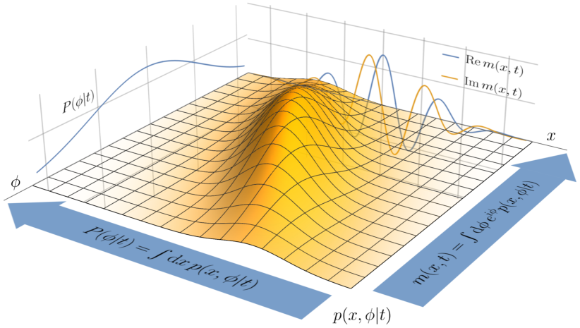
Figure 1: The solution (19) for representative parameter values. The PPD $p(\bm{x},\phi|t)$ is the fundamental quantity out of which the phase density $P(\phi|t)$ and magnetization density $m(\bm{x},t)$ emerge upon marginalization/averaging.

Discussion

The NMR signal can be expressed as $E(t)=\int{\rm d}\phi\,{e}^{{i}\phi}P(\phi|t)$, and in turn $P(\phi|t)=\int{\rm d}^{3}x\,p(\bm{x},\phi|t)$; see Fig. 1. Hence the evolution (7) of the PPD $p(\bm{x},\phi|t)$ furnishes insight into how the (global) phase distribution $P(\phi|t)$ develops.

The phase distribution $P(\phi|t)$ is in general not Gaussian, although it is often approximated to be so, be it directly Neuman (1974); Murday and Cotts (1968); Grebenkov (2007), or indirectly via asserting that it obeys diffusion along $\phi$ Lin (2015). Recently, it was proposed that approximating the conditional probability $p(\phi|\bm{x},t)$ to be Gaussian rather than the global phase distribution $P(\phi|t)$ is closer to reality Ziener et al. (2018). The nonzero cumulants, of which there are two, were furthermore stated to obey certain partial differential equations. These equations, as well as those of higher nonvanishing cumulants, are encompassed by the PPD evolution (7) upon substitution of $p(\bm{x},\phi|t)=p(\phi|\bm{x},t)/\rho(\bm{x}|t)$:

$$\partial_{t}p(\phi|\bm{x},t) =\Delta^{\!\rm Br}_{*}p(\phi|\bm{x},t)-\omega(\bm{x},t)\partial_{\phi}p(\phi|\bm{x},t)\,$$ (21)

with the operator

$$\Delta^{\!\rm Br}_{*} =\rho_{\rm st}^{-1}(\bm{x})\Delta^{\!\rm Br}\rho_{\rm st}(\bm{x})+2\left(\nabla\ln\frac{\rho(\bm{x}|t)}{\rho_{\rm st}(\bm{x})}\right)\cdot\nabla\,,$$ (22)

and $\rho_{\rm st}(\bm{x})\propto{e}^{-V(\bm{x})}$, generalizing them to the non-stationary non-Gaussian case. Note that a Hookean confinement (19), including the limit $\mathbf{C}\to 0$, constitutes the general problem (under a linear field gradient, that is) where the distribution $p(\phi|\bm{x},t)$ of phase angles is actually Gaussian, since it uses the most general stationary Gaussian process in Eq. (14).

Upon the simple linear coordinate transformation $\tilde{\phi}=\lambda\phi$, the probability density $\tilde{p}(\bm{x},\tilde{\phi}|t)=\lambda^{-1}p(\bm{x},\phi|t)$ is found to obey Eq. (7) with the replacement $\omega(\bm{x},t)\to\lambda\omega(\bm{x},t)$. In other words, once the PPD $p(\bm{x},\phi|t)$ evolving under field $\omega(\bm{x},t)$ is known, solutions under $\lambda\omega(\bm{x},t)$ for all $\lambda$ follow trivially as $\lambda^{-1}p(\bm{x},\lambda^{-1}\phi|t)$. In contrast, magnetization densities $m(\bm{x},t)$ solving the transverse Bloch-Torrey equation (BTE) do not exhibit such a feature in any obvious way Stoller et al. (1991); Herberthson et al. (2017). This is closely related to the previously explained fact that $p(\bm{x},\phi|t)$ comprises the solutions to an entire family of transverse BTEs.

Finally, we note that even though the precession field $\omega(\bm{x},t)$ was written as a function of position, a dependence on the phase angle $\phi$ can be accounted for simply by swapping the last term in Eq. (7) with $-\partial_{\phi}\omega(\bm{x},\phi,t)p(\bm{x},\phi|t)$. While it is not the typical scenario, this version may be applicable to experiments where quasi-instantaneous RF pulses rotate spins around an axis within the transverse plane until they are back in the transverse plane at an angle that is a function of its initial value.

In closing, we introduced the PPD and its evolution (7) as a framework for studying the dynamics of magnetic moments transverse to a polarizing field with significant conceptual benefits over the traditional BTE.