Interior angle sums of geodesic triangles in $\mathbf{S}^{2}\!\times\!\mathbf{R}$ and $\mathbf{H}^{2}\!\times\!\mathbf{R}$ geometries

Abstract

In the present paper we study $\mathbf{S}^{2}\!\times\!\mathbf{R}$ and $\mathbf{H}^{2}\!\times\!\mathbf{R}$ geometries, which are homogeneous Thurston 3-geometries. We analyse the interior angle sums of geodesic triangles in both geometries and prove, that in $\mathbf{S}^{2}\!\times\!\mathbf{R}$ space it can be larger or equal than $\pi$ and in $\mathbf{H}^{2}\!\times\!\mathbf{R}$ space the angle sums can be less or equal than $\pi$.

In our work we will use the projective model of $\mathbf{S}^{2}\!\times\!\mathbf{R}$ and $\mathbf{H}^{2}\!\times\!\mathbf{R}$ geometries described by E. Molnár in [6].

1 Introduction

A geodesic triangle in Riemannian geometry and more generally in metric geometry a figure consisting of three different points together with the pairwise-connecting geodesic curves. The points are known as the vertices, while the geodesic curve segments are known as the sides of the triangle.

In the geometries of constant curvature $\mathbf{E}^{3}$, $\mathbf{H}^{3}$, $\mathbf{S}^{3}$ the well-known sums of the interior angles of geodesic triangles characterize the space. It is related to the Gauss-Bonnet theorem which states that the integral of the Gauss curvature on a compact $2$-dimensional Riemannian manifold $M$ is equal to $2\pi\chi(M)$ where $\chi(M)$ denotes the Euler characteristic of $M$. This theorem has a generalization to any compact even-dimensional Riemannian manifold (see e.g. [2], [4]).

Remark 1.1

In the Thurston spaces can be introduced in a natural way (see [6]) translation curves. These curves are simpler than geodesics and differ from them in $\mathbf{Nil}$, $\widetilde{\mathbf{S}\mathbf{L}_{2}\mathbf{R}}$ and $\mathbf{Sol}$ geometries. In $\mathbf{E}^{3}$, $\mathbf{S}^{3}$, $\mathbf{H}^{3}$, $\mathbf{S}^{2}\!\times\!\mathbf{R}$ and $\mathbf{H}^{2}\!\times\!\mathbf{R}$ geometries the mentioned curves coincide with each other ([1], [3], [14], [20]).

In [3] we investigated the angle sums of translation and geodesic triangles in $\widetilde{\mathbf{S}\mathbf{L}_{2}\mathbf{R}}$ geometry and proved that the possible sum of the interior angles in a translation triangle must be greater or equal than $\pi$. However, in geodesic triangles this sum is less, greater or equal to $\pi$.

In [19] we considered the analogous problem for geodesic triangles in $\mathbf{Nil}$ geometry and proved that the sum of the interior angles of geodesic triangles in $\mathbf{Nil}$ space is larger, less or equal than $\pi$. In [1] K. Brodaczewska showed, that sum of the interior angles of translation triangles of the $\mathbf{Nil}$ space is larger or equal than $\pi$.

In [20] we studied the interior angle sums of translation triangles in $\mathbf{Sol}$ geometry and proved that the possible sum of the interior angles in a translation triangle must be greater or equal than $\pi$. Further interesting properties of translation triangles and tetrahedra are described in [14].

However, in $\mathbf{S}^{2}\!\times\!\mathbf{R}$, $\mathbf{H}^{2}\!\times\!\mathbf{R}$ and $\mathbf{Sol}$ Thurston geometries there are no result concerning the angle sums of geodesic triangles. Therefore, it is interesting to study this question in the above three geometries.

In the present paper, we are interested in geodesic triangles in $\mathbf{S}^{2}\!\times\!\mathbf{R}$ and $\mathbf{H}^{2}\!\times\!\mathbf{R}$ spaces [12, 21].

In Section 2 we describe the projective model and the isometry group of the considered geometries, moreover, we give an overview about its geodesic curves. In Section 3 we study the $\mathbf{S}^{2}\!\times\!\mathbf{R}$ and $\mathbf{H}^{2}\!\times\!\mathbf{R}$ geodesic triangles and their properties.

2 Projective model of $\mathbf{H}^{2}\!\times\!\mathbf{R}$ and $\mathbf{S}^{2}\!\times\!\mathbf{R}$ spaces

E. Molnár has shown in [6], that the homogeneous 3-spaces have a unified interpretation in the projective 3-sphere $\mathcal{PS}^{3}(\mathbf{V}^{4},\boldsymbol{V}_{4},\mathbf{R})$. In our work we shall use this projective model of $\mathbf{S}^{2}\!\times\!\mathbf{R}$ and $\mathbf{H}^{2}\!\times\!\mathbf{R}$ geometries. The Cartesian homogeneous coordinate simplex $E_{0}(\mathbf{e}_{0})$,$E_{1}^{\infty}(\mathbf{e}_{1})$,$E_{2}^{\infty}(\mathbf{e}_{2})$, $E_{3}^{\infty}(\mathbf{e}_{3})$, $(\{\mathbf{e}_{i}\}\subset\mathbf{V}^{4}$  with the unit point $E(\mathbf{e}=\mathbf{e}_{0}+\mathbf{e}_{1}+\mathbf{e}_{2}+\mathbf{e}_{3}))$ which is distinguished by an origin $E_{0}$ and by the ideal points of coordinate axes, respectively. Moreover, $\mathbf{y}=c\mathbf{x}$ with $0<c\in\mathbf{R}$ (or $c\in\mathbf{R}\setminus\{0\})$ defines a point $(\mathbf{x})=(\mathbf{y})$ of the projective 3-sphere $\mathcal{P}\mathcal{S}^{3}$ (or that of the projective space $\mathcal{P}^{3}$ where opposite rays $(\mathbf{x})$ and $(-\mathbf{x})$ are identified). The dual system $\{(\boldsymbol{e}^{i})\}\subset\boldsymbol{V}_{4}$ describes the simplex planes, especially the plane at infinity $(\boldsymbol{e}^{0})=E_{1}^{\infty}E_{2}^{\infty}E_{3}^{\infty}$, and generally, $\boldsymbol{v}=\boldsymbol{u}\frac{1}{c}$ defines a plane $(\boldsymbol{u})=(\boldsymbol{v})$ of $\mathcal{P}\mathcal{S}^{3}$ (or that of $\mathcal{P}^{3}$). Thus $0=\mathbf{x}\boldsymbol{u}=\mathbf{y}\boldsymbol{v}$ defines the incidence of point $(\mathbf{x})=(\mathbf{y})$ and plane $(\boldsymbol{u})=(\boldsymbol{v})$, as $(\mathbf{x})\text{I}(\boldsymbol{u})$ also denotes it. Thus $\mathbf{S}^{2}\!\times\!\mathbf{R}$ can be visualized in the affine 3-space $\mathbf{A}^{3}$ (so in $\mathbf{E}^{3}$) as well.

2.1 Geodesic curves in $\mathbf{S}^{2}\!\times\!\mathbf{R}$ space

In this section we recall the important notions and results from the papers [6], [10], [13], [15], [16].

The well-known infinitezimal arc-length square at any point of $\mathbf{S}^{2}\!\times\!\mathbf{R}$ as follows

$$\begin{gathered}(ds)^{2}=\frac{(dx)^{2}+(dy)^{2}+(dz)^{2}}{x^{2}+y^{2}+z^{2}}.\end{gathered}$$ (2.1)

We shall apply the usual geographical coordiantes $(\phi,\theta),\leavevmode\nobreak\ (-\pi<\phi\leq\pi,\leavevmode\nobreak\ -\frac{\pi}{2}\leq\theta\leq\frac{\pi}{2})$ of the sphere with the fibre coordinate $t\in\mathbf{R}$. We describe points in the above coordinate system in our model by the following equations:

$$x^{0}=1,\ \ x^{1}=e^{t}\cos{\phi}\cos{\theta},\ \ x^{2}=e^{t}\sin{\phi}\cos{\theta},\ \ x^{3}=e^{t}\sin{\theta}.$$ (2.2)

Then we have $x=\frac{x^{1}}{x^{0}}=x^{1}$, $y=\frac{x^{2}}{x^{0}}=x^{2}$, $z=\frac{x^{3}}{x^{0}}=x^{3}$, i.e. the usual Cartesian coordinates. We obtain by [6] that in this parametrization the infinitezimal arc-length square at any point of $\mathbf{S}^{2}\!\times\!\mathbf{R}$ is the following

$$\begin{gathered}(ds)^{2}=(dt)^{2}+(d\phi)^{2}\cos^{2}\theta+(d\theta)^{2}.\end{gathered}$$ (2.3)

The geodesic curves of $\mathbf{S}^{2}\!\times\!\mathbf{R}$ are generally defined as having locally minimal arc length between their any two (near enough) points. The equation systems of the parametrized geodesic curves $\gamma(t(\tau),\phi(\tau),\theta(\tau))$ in our model can be determined by the general theory of Riemann geometry (see [4], [16]).

Then by (2.2) we get with $c=\sin{v}$, $\omega=\cos{v}$ the equation systems of a geodesic curve, visualized in Fig. 3 in our Euclidean model:

$$\begin{gathered}x(\tau)=e^{\tau\sin{v}}\cos{(\tau\cos{v})},\\ y(\tau)=e^{\tau\sin{v}}\sin{(\tau\cos{v})}\cos{u},\\ z(\tau)=e^{\tau\sin{v}}\sin{(\tau\cos{v})}\sin{u},\\ -\pi<u\leq\pi,\ \ -\frac{\pi}{2}\leq v\leq\frac{\pi}{2}.\end{gathered}$$ (2.4)

Definition 2.1

The distance $d(P_{1},P_{2})$ between the points $P_{1}$ and $P_{2}$ is defined by the arc length of the shortest geodesic curve from $P_{1}$ to $P_{2}$.

2.2 Geodesic curves of $\mathbf{H}^{2}\!\times\!\mathbf{R}$ geometry

In this section we recall the important notions and results from the papers [6], [11], [17].

The points of $\mathbf{H}^{2}\!\times\!\mathbf{R}$ space, forming an open cone solid in the projective space $\mathcal{P}^{3}$, are the following:

$$\mathbf{H}^{2}\!\times\!\mathbf{R}:=\big{\{}X(\mathbf{x}=x^{i}\mathbf{e}_{i})\in\mathcal{P}^{3}:-(x^{1})^{2}+(x^{2})^{2}+(x^{3})^{2}<0<x^{0},\leavevmode\nobreak\ x^{1}\big{\}}.$$

In this context E. Molnár [6] has derived the infinitezimal arc-length square at any point of $\mathbf{H}^{2}\!\times\!\mathbf{R}$ as follows

$$\begin{gathered}(ds)^{2}=\frac{1}{(-x^{2}+y^{2}+z^{2})^{2}}\cdot[(x)^{2}+(y)^{2}+(z)^{2}](dx)^{2}+\\ +2dxdy(-2xy)+2dxdz(-2xz)+[(x)^{2}+(y)^{2}-(z)^{2}](dy)^{2}+\\ +2dydz(2yz)+[(x)^{2}-(y)^{2}+(z)^{2}](dz)^{2}.\end{gathered}$$ (2.5)

This becomes simpler in the following special (cylindrical) coordiantes $(t,r,\alpha)$, $(r\geq 0,\leavevmode\nobreak\ -\pi<\alpha\leq\pi)$ with the fibre coordinate $t\in\mathbf{R}$. We describe points in our model by the following equations:

$$x^{0}=1,\ \ x^{1}=e^{t}\cosh{r},\ \ x^{2}=e^{t}\sinh{r}\cos{\alpha},\ \ x^{3}=e^{t}\sinh{r}\sin{\alpha}.$$ (2.6)

Then we have $x=\frac{x^{1}}{x^{0}}=x^{1}$, $y=\frac{x^{2}}{x^{0}}=x^{2}$, $z=\frac{x^{3}}{x^{0}}=x^{3}$, i.e. the usual Cartesian coordinates. We obtain by [6] that in this parametrization the infinitezimal arc-length square by (2.1) at any point of $\mathbf{H}^{2}\!\times\!\mathbf{R}$ is the following

$$\begin{gathered}(ds)^{2}=(dt)^{2}+(dr)^{2}+\sinh^{2}{r}(d\alpha)^{2}.\end{gathered}$$ (2.7)

The geodesic curves of $\mathbf{H}^{2}\!\times\!\mathbf{R}$ are generally defined as having locally minimal arc length between their any two (near enough) points. The equation systems of the parametrized geodesic curves $\gamma(t(\tau),r(\tau),\alpha(\tau))$ in our model can be determined by the general theory of Riemann geometry:

By (2.5) the second order differential equation system of the $\mathbf{H}^{2}\!\times\!\mathbf{R}$ geodesic curve is the following [17]:

$$\ddot{\alpha}+2\coth(r)\leavevmode\nobreak\ \dot{r}\dot{\alpha}=0,\leavevmode\nobreak\ \ddot{r}-\sinh(r)\cosh(r)\dot{\alpha}^{2}=0,\leavevmode\nobreak\ \ddot{t}=0,$$ (2.8)

from which we get first a line as ”geodesic hyperbola” on our model of $\mathbf{H}^{2}$ times a component on $\mathbf{R}$ each running with constant velocity $c$ and $\omega$, respectively:

$$t=c\cdot\tau,\ \ \alpha=0,\ \ r=\omega\cdot\tau,\ \ c^{2}+\omega^{2}=1.$$ (2.9)

We can assume, that the starting point of a geodesic curve is $(1,1,0,0)$, because we can transform a curve into an arbitrary starting point, moreover, unit velocity with ”geographic” coordinates $(u,v)$ can be assumed:

$$\begin{gathered}r(0)=\alpha(0)=t(0)=0;\ \ \dot{t}(0)=\sin{v},\ \dot{r}(0)=\cos{v}\cos{u},\dot{\alpha}(0)=\cos{v}\sin{u};\\ -\pi<u\leq\pi,\leavevmode\nobreak\ -\frac{\pi}{2}\leq v\leq\frac{\pi}{2}.\end{gathered}$$

Then by (2.6) we get with $c=\sin{v}$, $\omega=\cos{v}$ the equation systems of a geodesic curve, visualized in Fig. 8 in our Euclidean model [17]:

$$\begin{gathered}x(\tau)=e^{\tau\sin{v}}\cosh{(\tau\cos{v})},\\ y(\tau)=e^{\tau\sin{v}}\sinh{(\tau\cos{v})}\cos{u},\\ z(\tau)=e^{\tau\sin{v}}\sinh{(\tau\cos{v})}\sin{u},\\ -\pi<u\leq\pi,\ \ -\frac{\pi}{2}\leq v\leq\frac{\pi}{2}.\end{gathered}$$ (2.10)

Definition 2.2

The distance $d(P_{1},P_{2})$ between the points $P_{1}$ and $P_{2}$ is defined by the arc length of the geodesic curve from $P_{1}$ to $P_{2}$.

Remark 2.3

$\mathbf{S}^{2}\!\times\!\mathbf{R}$ and $\mathbf{H}^{2}\!\times\!\mathbf{R}$ are affine metric spaces (affine-projective spaces – in the sense of the unified formulation of [6]). Therefore their linear, affine, unimodular, etc. transformations are defined as those of the embedding affine space.

3 Geodesic triangles

We consider $3$ points $A_{1}$, $A_{2}$, $A_{3}$ in the projective model of $X$ space (see Section 2) $(X\in\{\mathbf{S}^{2}\!\times\!\mathbf{R},\mathbf{H}^{2}\!\times\!\mathbf{R}\}$. The geodesic segments $a_{k}$ connecting the points $A_{i}$ and $A_{j}$ $(i<j,\leavevmode\nobreak\ i,j,k\in\{1,2,3\},k\neq i,j$) are called sides of the geodesic triangle with vertices $A_{1}$, $A_{2}$, $A_{3}$ (see Fig. 1, 2).

In Riemannian geometries the infinitesimal arc-lenght square (see (2.1) and (2.5)) is used to define the angle $\theta$ between two geodesic curves. If their tangent vectors in their common point are $\mathbf{u}$ and $\mathbf{v}$ and $g_{ij}$ are the components of the metric tensor then

$$\cos(\theta)=\frac{u^{i}g_{ij}v^{j}}{\sqrt{u^{i}g_{ij}u^{j}\leavevmode\nobreak\ v^{i}g_{ij}v^{j}}}$$ (3.1)

It is clear by the above definition of the angles and by the infinitesimal arc-lenght squares that the angles are the same as the Euclidean ones at the starting point of the geodesics.

Considering a geodesic triangle $A_{1}A_{2}A_{3}$ we can assume by the homogeneity of the considered geometries that one of its vertex coincide with the point $A_{1}=(1,1,0,0)$ and the other two vertices are $A_{2}=(1,x^{2},y^{2},z^{2})$ and $A_{3}=(1,x^{3},y^{3},z^{3})$.

We will consider the interior angles of geodesic triangles that are denoted at the vertex $A_{i}$ by $\omega_{i}$ $(i\in\{1,2,3\})$. We note here that the angle of two intersecting geodesic curves depends on the orientation of their tangent vectors.

3.1 Interior angle sums in $\mathbf{S}^{2}\!\times\!\mathbf{R}$ geometry

In order to determine the interior angles of a geodesic triangle $A_{1}A_{2}A_{3}$ and its interior angle sum $\sum_{i=1}^{3}(\omega_{i})$, we define isometric transformations $\mathbf{T}^{\mathbf{S}^{2}\!\times\!\mathbf{R}}_{A_{i}}$, $(i\in\{2,3\}$, as elements of the isometry group of $\mathbf{S}^{2}\!\times\!\mathbf{R}$ geometry, that maps the $A_{i}$ onto $A_{1}$). Let the isometrie $\mathbf{T}^{\mathbf{S}^{2}\!\times\!\mathbf{R}}_{A_{2}}$ be given by the composition of some special types of $\mathbf{S}^{2}\!\times\!\mathbf{R}$ isometries, which transforms a fixed $A_{2}=(1,x_{2},y_{2},z_{2})$ point of $\mathbf{S}^{2}\!\times\!\mathbf{R}$ into $(1,1,0,0)$ (up to a positive determinant factor):

${\mathcal{T}}=({\bf Id.},T)$ is a fibre translation,

$$\begin{gathered}A_{2}=(1,x_{2},y_{2},z_{2})\rightarrow A_{2}^{\mathcal{T}}=(1,x_{2}^{\prime},y_{2}^{\prime},z_{2}^{\prime})=\\ =A_{2}^{\mathcal{T}}=\Big{(}1,\frac{x_{2}}{\sqrt{x_{2}^{2}+y_{2}^{2}+z_{2}^{2}}},\frac{y_{2}}{\sqrt{x_{2}^{2}+y_{2}^{2}+z_{2}^{2}}},\frac{z_{2}}{\sqrt{x_{2}^{2}+y_{2}^{2}+z_{2}^{2}}}\Big{)}.\end{gathered}$$ (3.2)

($A_{2}^{{\mathcal{T}}}$ has $0$ fibre coordinate). ${\mathcal{R}_{x}}=({\bf R_{x}},0)$ is a special rotation about $x$ axis with $0$ fibre translation, which moves the point $(1,x_{2}^{\prime},y_{2}^{\prime},z_{2}^{\prime})$ into the $[x,y]$ plane.

$$\begin{gathered}A_{2}^{{\mathcal{T}}}=(1,x_{2}^{\prime},y_{2}^{\prime},z_{2}^{\prime})\rightarrow A_{2}^{{\mathcal{T}}{\mathcal{R}_{x}}}=(1,x_{2}^{\prime\prime},y_{2}^{\prime\prime},0)=\\ =A_{2}^{{\mathcal{T}}{\mathcal{R}_{x}}}=(1,x_{2}^{\prime},\sqrt{y_{2}^{\prime 2}+z_{2}^{\prime 2}},0).\end{gathered}$$ (3.3)

Similarly, ${\mathcal{R}_{z}}=({\bf R_{z}},0)$ is a special rotation about $z$ axis with $0$ fibre translation, which moves the point $(1,x_{2}^{\prime\prime},y_{2}^{\prime\prime},0)$ into the $(1,1,0,0)$ point.

$$\begin{gathered}A_{2}^{\mathcal{T}{\mathcal{R}_{x}}}=(1,x_{2}^{\prime\prime},y_{2}^{\prime\prime},0)\rightarrow A_{2}^{{\mathcal{T}}{\mathcal{R}_{x}}{\mathcal{R}_{z}}}=(1,1,0,0).\end{gathered}$$ (3.4)

Finally we apply the inverse transformation $\mathcal{R}^{-1}_{x}$ of rotation $\mathcal{R}_{x}$ because of that the geodesic curve $g(A_{1},A_{2})$ between the points $A_{1}$ and $A_{2}$ and its image $g(A_{1}^{2},A_{1})$ under the transformation ${\mathcal{T}}{\mathcal{R}_{x}}{\mathcal{R}_{z}}{\mathcal{R}^{-1}_{x}}$ lie in the same plane in Euclidean sense. The matrix of the above transformation $\mathbf{T}^{\mathbf{S}^{2}\!\times\!\mathbf{R}}_{A_{2}}={\mathcal{T}}{\mathcal{R}_{x}}{\mathcal{R}_{z}}{\mathcal{R}^{-1}_{x}}$ is the following:

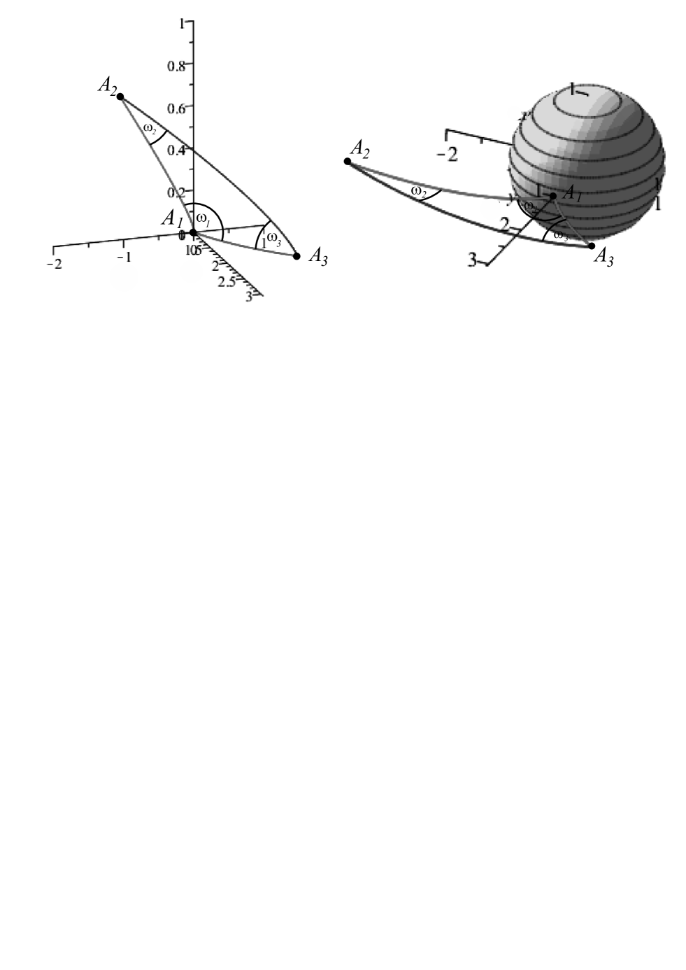
Figure 1: Geodesic triangle with vertices $A_{1}=(1,1,0,0)$, $A_{2}=(1,3,-2,1)$, $A_{3}=(1,2,1,0)$ in $\mathbf{S}^{2}\!\times\!\mathbf{R}$ geometry.

$\mathbf{T}^{\mathbf{S}^{2}\!\times\!\mathbf{R}}_{A_{2}}=$

$$\begin{gathered}=\begin{pmatrix}1&0&0&0\\ 0&\frac{x_{2}}{(x_{2})^{2}+(y_{2})^{2}+(z_{2})^{2}}&\frac{-y_{2}}{(x_{2})^{2}+(y_{2})^{2}+(z_{2})^{2}}&\frac{-z_{2}}{(x_{2})^{2}+(y_{2})^{2}+(z_{2})^{2}}\\ 0&\frac{y_{2}}{(x_{2})^{2}+(y_{2})^{2}+(z_{2})^{2}}&\frac{(y_{2})^{2}x_{2}+(z_{2})^{2}\sqrt{(x_{2})^{2}+(y_{2})^{2}+(z_{2})^{2}}}{((x_{2})^{2}+(y_{2})^{2}+(z_{2})^{2})((y_{2})^{2}+(z_{2})^{2})}&\frac{-y_{2}z_{2}(-x_{2}+\sqrt{(x_{2})^{2}+(y_{2})^{2}+(z_{2})^{2}})}{((x_{2})^{2}+(y_{2})^{2}+(z_{2})^{2})((y_{2})^{2}+(z_{2})^{2})}\\ 0&\frac{z_{2}}{(x_{2})^{2}+(y_{2})^{2}+(z_{2})^{2}}&\frac{(y_{2})z_{2}(-x_{2}+\sqrt{(x_{2})^{2}+(y_{2})^{2}+(z_{2})^{2}})}{((x_{2})^{2}+(y_{2})^{2}+(z_{2})^{2})((y_{2})^{2}+(z_{2})^{2})}&\frac{(z_{2})^{2}x_{2}+(y_{2})^{2}\sqrt{(x_{2})^{2}+(y_{2})^{2}+(z_{2})^{2}})}{((x_{2})^{2}+(y_{2})^{2}+(z_{2})^{2})((y_{2})^{2}+(z_{2})^{2})}\end{pmatrix},\end{gathered}$$ (3.5)

and the images $\mathbf{T}^{\mathbf{S}^{2}\!\times\!\mathbf{R}}_{A_{2}}(A_{i})$ of the vertices $A_{i}$ $(i\in\{1,2,3\})$ are the following (see also Fig. 2):

$$\begin{gathered}\mathbf{T}^{\mathbf{S}^{2}\!\times\!\mathbf{R}}_{A_{2}}(A_{1})=A_{1}^{2}=\\ =\Big{(}1,\frac{x_{2}}{(x_{2})^{2}+(y_{2})^{2}+(z_{2})^{2}},\frac{-y_{2}}{(x_{2})^{2}+(y_{2})^{2}+(z_{2})^{2}},\frac{-z_{2}}{(x_{2})^{2}+(y_{2})^{2}+(z_{2})^{2}}\Big{)},\\ \mathbf{T}^{\mathbf{S}^{2}\!\times\!\mathbf{R}}_{A_{2}}(A_{2})=A_{2}^{2}=(1,1,0,0),\\ \mathbf{T}^{\mathbf{S}^{2}\!\times\!\mathbf{R}}_{A_{2}}(A_{3})=A_{3}^{2}=\Big{(}1,\frac{x_{2}x_{3}+y_{2}y_{3}}{(x_{2})^{2}+(y_{2})^{2}+(z_{2})^{2}},\\ \frac{y_{3}(z_{2})^{2}\sqrt{(x_{2})^{2}+(y_{2})^{2}+(z_{2})^{2}}+x_{2}(y_{2})^{2}y_{3}-x_{3}(y_{2})^{3}-x_{3}y_{2}(z_{2})^{2}}{((y_{2})^{2}+(z_{2})^{2})((x_{2})^{2}+(y_{2})^{2}+(z_{2})^{2})},\\ -\frac{z_{2}(y_{3}y_{2}(\sqrt{(x_{2})^{2}+(y_{2})^{2}+(z_{2})^{2}}-x_{2})+x_{3}(y_{2})^{2}+x_{3}(z_{2})^{2})}{((y_{2})^{2}+(z_{2})^{2})((x_{2})^{2}+(y_{2})^{2}+(z_{2})^{2})}\Big{)}.\end{gathered}$$ (3.6)

Remark 3.1

More informations about the isometry group of $\mathbf{S}^{2}\!\times\!\mathbf{R}$ and about its discrete subgroups can be found in [15] and [16].

Similarly to the above computation we get that the images $\mathbf{T}^{\mathbf{S}^{2}\!\times\!\mathbf{R}}_{A_{3}}(A_{i})$ of the vertices $A_{i}$ $(i\in\{1,2,3\})$ are the following (see also Fig. 2):

$$\begin{gathered}\mathbf{T}^{\mathbf{S}^{2}\!\times\!\mathbf{R}}_{A_{3}}(A_{1})=A_{1}^{3}=\Big{(}1,\frac{x_{3}}{(x_{3})^{2}+(y_{3})^{2}},\frac{-y_{3}}{(x_{3})^{2}+(y_{3})^{2}},0\Big{)},\\ \mathbf{T}^{\mathbf{S}^{2}\!\times\!\mathbf{R}}_{A_{3}}(A_{3})=A_{3}^{3}=A_{1}=(1,1,0,0),\\ \mathbf{T}^{\mathbf{S}^{2}\!\times\!\mathbf{R}}_{A_{3}}(A_{2})=A_{2}^{3}=\Big{(}1,\frac{x_{2}x_{3}+y_{2}y_{3}}{(x_{3})^{2}+(y_{3})^{2}},\frac{x_{3}y_{2}-x_{2}y_{3}}{(x_{3})^{2}+(y_{3})^{2}},\frac{z_{2}}{\sqrt{(x_{3})^{2}+(y_{3})^{2}}}\Big{)}.\end{gathered}$$ (3.7)

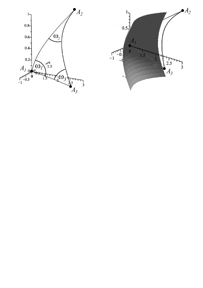
Figure 2: Geodesic triangle with vertices $A_{1}=(1,1,0,0)$, $A_{2}=(1,3,-2,1)$, $A_{3}=(1,2,1,0)$ in $\mathbf{S}^{2}\!\times\!\mathbf{R}$ geometry, and transformed images of its geodesic side segments.

Our aim is to determine angle sum $\sum_{i=1}^{3}(\omega_{i})$ of the interior angles of geodesic triangles $A_{1}A_{2}A_{3}$ (see Fig. 1, 2). We have seen that $\omega_{1}$ and the angle of geodesic curves with common point at the vertex $A_{1}$ is the same as the Euclidean one therefore can be determined by usual Euclidean sense.

The $\mathbf{T}^{\mathbf{S}^{2}\!\times\!\mathbf{R}}_{A_{i}}$ $(i=2,3)$ are isometries in $\mathbf{S}^{2}\!\times\!\mathbf{R}$ geometry thus $\omega_{i}$ is equal to the angle $(g(A_{i}^{i},A_{1}^{i}),g(A_{i}^{i},A_{j}^{i}))\angle$ $(i,j=2,3$, $i\neq j)$ (see Fig. 2) where $g(A_{i}^{i},A_{1}^{i})$, $g(A_{i}^{i},A_{j}^{i})$ are oriented geodesic curves $(A_{1}=A_{2}^{2}=A_{3}^{3})$ and $\omega_{1}$ is equal to the angle $(g(A_{1},A_{2}),g(A_{1},A_{3}))\angle$ where $g(A_{1},A_{2})$, $g(A_{1},A_{3})$ are also oriented geodesic curves.

We denote the oriented unit tangent vectors of the oriented geodesic curves $g(A_{1},A_{i}^{j})$ with $\mathbf{t}_{i}^{j}$ where $(i,j)\in\{(1,3),(1,2),(2,3),(3,2),(3,0),(2,0)\}$ and $A_{3}^{0}=A_{3}$, $A_{2}^{0}=A_{2}$. The Euclidean coordinates of $\mathbf{t}_{i}^{j}$ (see Section 2.1) are :

$$\mathbf{t}_{i}^{j}=(\sin(v_{i}^{j}),\cos(v_{i}^{j})\cos(u_{i}^{j}),\cos(v_{i}^{j})\sin(u_{i}^{j})).$$ (3.8)

In order to obtain the angle of two geodesic curves $g{(A_{1},A_{i}^{j}})$ and $g{(A_{1},A_{k}^{l})}$ ($(i,j)\neq(k,l)$; $(i,j),(k,l)\in\{(1,3),(1,2),(2,3),(3,2),(3,0),(2,0)\})$ intersected at the vertex $A_{1}$ we need to determine their tangent vectors $\mathbf{t}_{s}^{r}$ $((s,r)\in\{(1,3),(1,2),$ $(2,3),(3,2),(3,0),(2,0)\})$ (see (3.8)) at their starting point $A_{1}$. From (3.8) follows that a tangent vector at the origin is given by the parameters $u$ and $v$ of the corresponding geodesic curve (see (2.10)) that can be determined from the homogeneous coordinates of the endpoint of the geodesic curve as the following Lemma shows:

Lemma 3.1

Let $(1,x,y,z)$ $(x,y,z\in\mathbf{R},x^{2}+y^{2}+z^{2}\neq 0)$ be the homogeneous coordinates of the point $P\in\mathbf{S}^{2}\!\times\!\mathbf{R}$. The paramerters of the corresponding geodesic curve $g{(A_{1},P)}$ are the following:

1. $y,z\in\mathbf{R}\setminus\{0\}$ and $x^{2}+y^{2}+z^{2}\neq 1$;

   $$\begin{gathered}v=\mathrm{arctan}\Big{(}\frac{\log\sqrt{x^{2}+y^{2}+z^{2}}}{\mathrm{arccos}\frac{x}{\sqrt{x^{2}+y^{2}+z^{2}}}}\Big{)},\leavevmode\nobreak\ u=\mathrm{arctan}\Big{(}\frac{z}{y}\Big{)},\\ \tau=\frac{\log\sqrt{x^{2}+y^{2}+z^{2}}}{\sin v},\leavevmode\nobreak\ \text{where}\leavevmode\nobreak\ -\pi<u\leq\pi,\leavevmode\nobreak\ -\pi/2\leq v\leq\pi/2,\leavevmode\nobreak\ \tau\in\mathbf{R}^{+}.\end{gathered}$$ (3.9)

2. $y=0$, $z\neq 0$ and $x^{2}+z^{2}\neq 1$;

   $$\begin{gathered}u=\frac{\pi}{2},\leavevmode\nobreak\ v=\mathrm{arctan}\Big{(}\frac{\log\sqrt{x^{2}+z^{2}}}{\mathrm{arccos}\frac{x}{\sqrt{x^{2}+z^{2}}}}\Big{)},\\ \tau=\frac{\log\sqrt{x^{2}+z^{2}}}{\sin v},\leavevmode\nobreak\ \text{where}\leavevmode\nobreak\ -\pi/2\leq v\leq\pi/2,\leavevmode\nobreak\ \tau\in\mathbf{R}^{+}.\end{gathered}$$ (3.10)

3. $y=0$, $z\neq 0$ and $x^{2}+z^{2}=1$;

   $$\begin{gathered}u=\frac{\pi}{2},\leavevmode\nobreak\ v=0,\leavevmode\nobreak\ \tau=\arccos(x),\leavevmode\nobreak\ \tau\in\mathbf{R}^{+}.\end{gathered}$$ (3.11)

4. $y,z=0$;

   $$u=0,\leavevmode\nobreak\ v=\frac{\pi}{2},\leavevmode\nobreak\ \tau=\log\sqrt{x^{2}+y^{2}+z^{2}},\leavevmode\nobreak\ \tau\in\mathbf{R}^{+}.$$ (3.12)

5. $x=0,\leavevmode\nobreak\ y=0$ and $z\neq 1$;

   $$\begin{gathered}u=\frac{\pi}{2},\leavevmode\nobreak\ v=\mathrm{arctan}\frac{2\log|z|}{\pi},\leavevmode\nobreak\ \tau=\frac{\log|z|}{\sin v},\\ -\pi/2\leq v\leq\pi/2,\leavevmode\nobreak\ \tau\in\mathbf{R}^{+}.\end{gathered}$$ (3.13)

$\square$

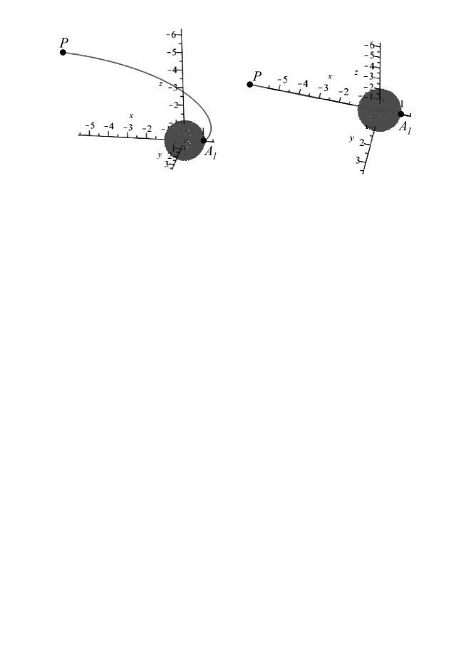
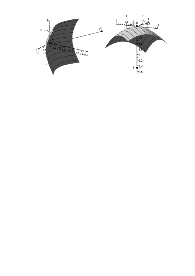
Figure 3: Geodesic curve $g(A_{1},P)$ ($A_{1}=(1,1,0,0)$ and $P\in\mathbf{S}^{2}\!\times\!\mathbf{R}$) with “base plane”, the plane of a geodesic curve contain the origin $E_{0}=(1,0,0,0)$ of the model.

We obtain directly from the (2.4) equations of the geodesic curves the following

Lemma 3.2

Let $P$ be an arbitrary point and $g(A_{1},P)$ ($A_{1}=(1,1,0,0)$) is a geodesic curve in the considered model of $\mathbf{S}^{2}\!\times\!\mathbf{R}$ geometry. The points of the geodesic curve $g(A_{1},P)$ and the centre of the model $E_{0}$ lie in a plane in Euclidean sense (see Fig. 3).     $\square$

Theorem 3.3

If the Euclidean plane of the vertices of a $\mathbf{S}^{2}\!\times\!\mathbf{R}$ geodesic triangle $A_{1}A_{2}A_{3}$ contains the centre of model $E_{0}$ then its interior angle sum is equal to $\pi$.

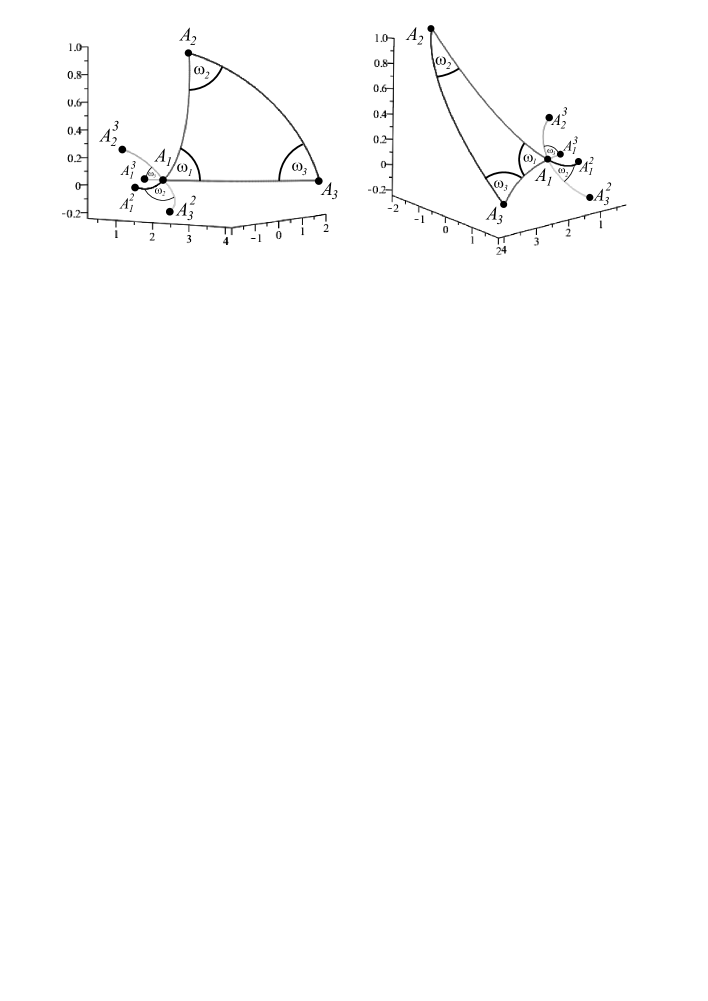
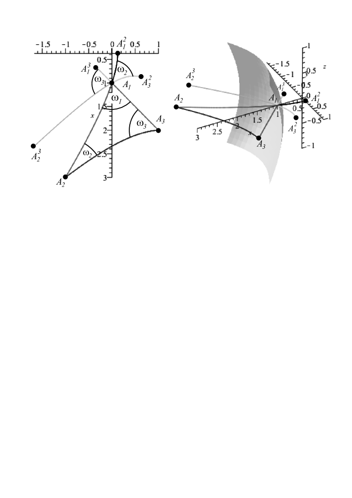
Figure 4: Geodesic triangle with vertices $A_{1}=(1,1,0,0)$, $A_{2}=(1,1,-3,0)$, $A_{3}=(1,2,1,0)$ in $\mathbf{S}^{2}\!\times\!\mathbf{R}$ geometry, and transformed images of its geodesic side segments. The geodesic curve segments $g{(A_{1},A_{2})}$, $g{(A_{2},A_{3})}$, $g({A_{1},A_{3}})$ lie on the coordinate plane $[x,y]$ and the interior angle sum of this geodesic triangle is $\sum_{i=1}^{3}(\omega_{i})=\pi$.

Proof: We can assume without loss of generality that the vertices $A_{1},A_{2},A_{3}$ of such a geodesic triangle lie in the $[x,y]$ plane of the model. Using the Lemma 3.2 we get, that the geodesic segments $A_{1}A_{2}$, $A_{1}A_{3}$ and $A_{2}A_{3}$ are containing by the [x,y] plane, too.

The $\mathbf{S}^{2}\!\times\!\mathbf{R}$ transformations $\mathbf{T}_{A_{2}}^{\mathbf{S}^{2}\!\times\!\mathbf{R}}$ and $\mathbf{T}_{A_{3}}^{\mathbf{S}^{2}\!\times\!\mathbf{R}}$ are isometries in $\mathbf{S}^{2}\!\times\!\mathbf{R}$ geometry thus $\omega_{2}$ is equal to the angle $(g(A_{2}^{2},A_{1}^{2}),g(A_{2}^{2},A_{3}^{2}))\angle$ (see Fig. 2, 4) of the oriented geodesic segments $g({A_{2}^{2},A_{1}^{2}})$, $g({A_{2}^{2},A_{3}^{2}})$ and $\omega_{3}$ is equal to the angle $(g(A_{3}^{3},A_{1}^{3}),g(A_{3}^{3}A_{2}^{3}))\angle$ of the oriented geodesic segments $g({A_{3}^{3},A_{1}^{3}})$ and $g({A_{3}^{3},A_{2}^{3}})$ $(A_{1}=A_{2}^{2}=A_{3}^{3}$).

Substituting the coordinates of the points $A_{i}^{j}$ (see (3.5), (3.6) and (3.7)) $((i,j)\in\{(1,3),(1,2),$ $(2,3),(3,2),(3,0),(2,0)\})$ to the appropriate equations (3.8-12) of Lemma 3.1, it is easy to see that

$$\begin{gathered}v_{2}^{0}=-v_{1}^{2},\leavevmode\nobreak\ u_{2}^{0}-u_{1}^{2}=\pm\pi\Rightarrow\mathbf{t}_{2}^{0}=-\mathbf{t}_{1}^{2},\\ v_{3}^{0}=-v_{1}^{3},\leavevmode\nobreak\ u_{3}^{0}-u_{1}^{3}=\pm\pi\Rightarrow\mathbf{t}_{3}^{0}=-\mathbf{t}_{1}^{3},\\ v_{3}^{2}=-v_{2}^{3},\leavevmode\nobreak\ u_{3}^{2}-u_{2}^{3}=\pm\pi\Rightarrow\mathbf{t}_{3}^{2}=-\mathbf{t}_{2}^{3}.\end{gathered}$$ (3.13)

The endpoints $T_{i}^{j}$ of the position vectors $\mathbf{t}_{i}^{j}=\overrightarrow{A_{1}T_{i}^{j}}$ lie on the unit sphere centred at the origin. The measure of angle $\omega_{i}$ $(i\in\{1,2,3\})$ of the vectors $\mathbf{t}_{i}^{j}$ and $\mathbf{t}_{r}^{s}$ is equal to the spherical distance of the corresponding points $T_{i}^{j}$ and $T_{r}^{s}$ on the unit sphere (see Fig. 4). Moreover, a direct consequence of equations (3.13) that each point pair ($T_{2}$, $T_{1}^{2}$), $(T_{3}$,$T_{1}^{3}$), ($T_{2}^{3}$,$T_{3}^{2}$) contains antipodal points related to the unit sphere with centre $A_{1}$.

Due to the antipodality $\omega_{1}=T_{2}A_{1}T_{3}\angle=T_{1}^{2}A_{1}T_{1}^{3}\angle$, therefore their corresponding spherical distances are equal, as well (see Fig. 4). Now, the sum of the interior angles $\sum_{i=1}^{3}(\omega_{i})$ can be considered as three consecutive spherical arcs $(T_{3}^{2}T_{1}^{2})$, $(T_{1}^{2}T_{1}^{3})$, $T_{1}^{3}T_{2}^{3})$. Since the points $T_{2}$, $T_{1}^{2}$, $T_{3}$, $T_{1}^{3}$, $T_{2}^{3}$, $T_{3}^{2}$ lie in the $[x,y]$ plane (see Lemma 3.2) the sum of these arc lengths is equal to the half of the circumference of the main circle on the unit sphere i.e. $\pi$. $\square$

Figure 5: Geodesic triangle with vertices $A_{1}=(1,1,0,0)$, $A_{2}=(1,3,-2,1)$, $A_{3}=(1,2,1,0)$ and the correspondig trihedron with base sphere of $\mathbf{S}^{2}\!\times\!\mathbf{R}$ geometry.

Figure 6: $S(\Delta(t))$ function related to parameters $x_{2}=3,y_{2}=-2,z_{2}=1$ $x_{3}=2\cdot t,y_{3}=1\cdot t,z_{3}=0$.

We can determine the interior angle sum of arbitrary geodesic triangle. In the following table we summarize some numerical data of interior angles of given geodesic triangles:

Table 1:   $A_{1}=(1,0,0,0)$, $A_{2}=(1,3,-2,1)$ $A_{3}/\omega_{i}$ $\omega_{1}$ $\omega_{2}$ $\omega_{3}$ $\sum_{i=1}^{3}(\omega_{i})$ $(1,2/\sqrt{5},1/\sqrt{5},0)$ $1.97206$ $0.26028$ $0.92635$ $3.15869$ $(1,2,1,0)$ $0.94654$ $0.68775$ $1.51707$ $3.15135$ $(1,4,2,0)$ $0.73193$ $1.29546$ $1.12123$ $3.14862$ $(1,12,6,0)$ $0.61470$ $1.99926$ $0.53246$ $3.14643$ $(1,2000,1000,0)$ $0.50628$ $2.52677$ $0.11050$ $3.14355$

By the above experiences and computations we obtain the following

Theorem 3.4

If the Euclidean plane of the vertices of a $\mathbf{S}^{2}\!\times\!\mathbf{R}$ geodesic triangle $A_{1}A_{2}A_{3}$ does not contain the centre of model $E_{0}$ then its interior angle sum is greater than $\pi$.

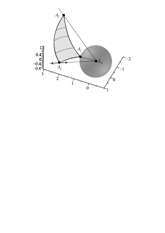
Proof: We can assume without loss of generality that the vertices $A_{1},A_{2}$ of such a geodesic triangle lie in the $[x,y]$ plane of the model. Using the Lemma 3.2 we get, that the geodesic segment $A_{i}A_{j}$, ($(i,j)\in\{(1,2),(1,3),2,3)\}$) is contained by the $A_{i}A_{j}E_{0}$ plane, therefore the sides of triangle $A_{1}A_{2}A_{3}$ lie in the boundary of trihedron given by the points $E_{0}$, $A_{1}$, $A_{2}$, $A_{3}$ (see Fig. 2 and 5). It is clear, that all types of geodesic triangles can be described by such a triangle. Therefore, it is sufficient investigate the interior angle sums of geodesic triangles where we fix two of the vertices, e.g. $A_{1}$ and $A_{2}$ and move the third vertex $A_{3}$ on the half straight line $E_{0}A_{3}$ with starting point $E_{0}\neq A_{3}(t)$.

Remark 3.2

It is well known, that if the vertices $A_{1},A_{2},A_{3}$ lie in a sphere of radius $R\in\mathbf{R}^{+}$ centred at $E_{0}$ then the interior angle sum of spherical triangle $A_{1}A_{2}A_{3}$ is greater than $\pi$.

Let $\Delta^{\mathbf{S}^{2}\!\times\!\mathbf{R}}(t)$ $(t\in\mathbf{R}^{+})$ denote the above geodesic triangle with interior angles at the vertex $A_{i}$ by $\omega_{i}(t)$ $(i\in\{1,2,3\})$.

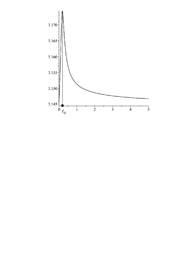
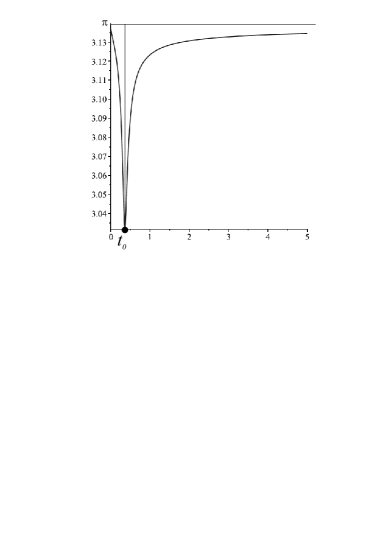
The interior angle sum function $S(\Delta(t))=\sum_{i=1}^{3}(\omega_{i}(t))$ can be determined related to the parameters $x_{2},y_{2},z_{2},x_{3},y_{3}\in\mathbf{R}$ by the formulas (2.4), (3.6), (3.7) and by the Lemma 3.1. Analyzing the above complicated continuous functions of single real variable $t$ we get that its maximum is achieved at a point $t_{0}\in(0,\infty)$ depending on given parameters. Moreover, $S(\Delta^{\mathbf{S}^{2}\!\times\!\mathbf{R}}(t))$ is stricly increasing on the interval $(0,t_{0})$, stricly decreasing on the interval $(t_{0},\infty)$ and

$$\lim_{t\rightarrow 0}S(\Delta^{\mathbf{S}^{2}\!\times\!\mathbf{R}}(t))=\pi,\leavevmode\nobreak\ \leavevmode\nobreak\ \leavevmode\nobreak\ \leavevmode\nobreak\ \lim_{t\rightarrow\infty}S(\Delta^{\mathbf{S}^{2}\!\times\!\mathbf{R}}(t))=\pi.\hskip 28.45274pt$$

In Fig. 6 we described the $S(\Delta^{\mathbf{S}^{2}\!\times\!\mathbf{R}}(t))$ function related to geodesic triangle $\Delta^{\mathbf{S}^{2}\!\times\!\mathbf{R}}(t)$ $(t\in(0,5))$ with vertices $A_{1}=(1,1,0,0)$, $A_{2}=(1,3,-2,1)$, $A_{3}=(1,2\cdot t,1\cdot t,0)$. Its maximum is achieved at $t_{0}\approx 0.19316$ where $S(\Delta^{\mathbf{S}^{2}\!\times\!\mathbf{R}}(t_{0}))\approx 3.17450$.       $\square$

Finally we get the following

Theorem 3.5

The sum of the interior angles of a geodesic triangle of $\mathbf{S}^{2}\!\times\!\mathbf{R}$ space is greater or equal to $\pi$.     $\square$

3.2 Interior angle sums in $\mathbf{H}^{2}\!\times\!\mathbf{R}$ geometry

Similarly to the $\mathbf{S}^{2}\!\times\!\mathbf{R}$ space we investigate the interior angles of a geodesic triangle $A_{1}A_{2}A_{3}$ and its interior angle sum $\sum_{i=1}^{3}(\omega_{i})$ in the $\mathbf{H}^{2}\!\times\!\mathbf{R}$ space. Therefore we define isometric transformations $\mathbf{T}^{\mathbf{H}^{2}\!\times\!\mathbf{R}}_{A_{i}}$, $(i\in\{2,3\})$, as elements of the isometry group of $\mathbf{H}^{2}\!\times\!\mathbf{R}$ geometry, that maps the $A_{i}$ onto the vertex $A_{1}$. Let the isometrie $\mathbf{T}^{\mathbf{H}^{2}\!\times\!\mathbf{R}}_{A_{2}}$ be given by the composition of some special types of $\mathbf{H}^{2}\!\times\!\mathbf{R}$ isometries, which transforms a fixed $A_{2}=(1,x_{2},y_{2},z_{2})$ point of $\mathbf{H}^{2}\!\times\!\mathbf{R}$ into $A_{1}=(1,1,0,0)$ (up to a positive determinant factor). The methods, the considered transformations and the determinations of their matrices are similar to the $\mathbf{S}^{2}\!\times\!\mathbf{R}$ case and are therefore not detailed here.

Figure 7: Geodesic triangle with vertices $A_{1}=(1,1,0,0)$, $A_{2}=(1,2,3/2,1)$, $A_{3}=(1,3,-1,0)$ in $\mathbf{H}^{2}\!\times\!\mathbf{R}$ geometry.

The images $\mathbf{T}^{\mathbf{H}^{2}\!\times\!\mathbf{R}}_{A_{2}}(A_{i})$ of the vertices $A_{i}$ $(i\in\{1,2,3\})$ are the following (see also Fig. 7, 9):

$$\begin{gathered}\mathbf{T}^{\mathbf{H}^{2}\!\times\!\mathbf{R}}_{A_{2}}(A_{1})=A_{1}^{2}=\\ =\Big{(}1,\frac{x_{2}}{(x_{2})^{2}-(y_{2})^{2}-(z_{2})^{2}},\frac{-y_{2}}{(x_{2})^{2}-(y_{2})^{2}-(z_{2})^{2}},\frac{-z_{2}}{(x_{2})^{2}-(y_{2})^{2}-(z_{2})^{2}}\Big{)},\\ \mathbf{T}^{\mathbf{H}^{2}\!\times\!\mathbf{R}}_{A_{2}}(A_{2})=A_{2}^{2}=(1,1,0,0),\\ \mathbf{T}^{\mathbf{H}^{2}\!\times\!\mathbf{R}}_{A_{2}}(A_{3})=A_{3}^{2}=\Big{(}1,\frac{x_{2}x_{3}-y_{2}y_{3}}{(x_{2})^{2}-(y_{2})^{2}-(z_{2})^{2}},\\ \frac{y_{3}(z_{2})^{2}\sqrt{(x_{2})^{2}-(y_{2})^{2}-(z_{2})^{2}}+x_{2}(y_{2})^{2}y_{3}-x_{3}(y_{2})^{3}-x_{3}y_{2}(z_{2})^{2}}{((y_{2})^{2}+(z_{2})^{2})((x_{2})^{2}-(y_{2})^{2}-(z_{2})^{2})},\\ -\frac{z_{2}(y_{3}y_{2}(\sqrt{(x_{2})^{2}-(y_{2})^{2}-(z_{2})^{2}}-x_{2})+x_{3}(y_{2})^{2}+x_{3}(z_{2})^{2})}{((y_{2})^{2}+(z_{2})^{2})((x_{2})^{2}-(y_{2})^{2}-(z_{2})^{2})}\Big{)}.\end{gathered}$$ (3.14)

Remark 3.3

More informations about the isometry group of $\mathbf{H}^{2}\!\times\!\mathbf{R}$ and about its discrete subgroups can be found in [17].

Similarly to the above computation we get that the images $\mathbf{T}^{\mathbf{H}^{2}\!\times\!\mathbf{R}}_{A_{3}}(A_{i})$ of the vertices $A_{i}$ $(i\in\{1,2,3\})$ are the following (see also Fig. 7, 9):

$$\begin{gathered}\mathbf{T}^{\mathbf{H}^{2}\!\times\!\mathbf{R}}_{A_{3}}(A_{1})=A_{1}^{3}=\Big{(}1,\frac{x_{3}}{(x_{3})^{2}-(y_{3})^{2}},\frac{-y_{3}}{(x_{3})^{2}-(y_{3})^{2}},0\Big{)},\\ \mathbf{T}^{\mathbf{H}^{2}\!\times\!\mathbf{R}}_{A_{3}}(A_{3})=A_{3}^{3}=A_{1}=(1,1,0,0),\\ \mathbf{T}^{\mathbf{H}^{2}\!\times\!\mathbf{R}}_{A_{3}}(A_{2})=A_{2}^{3}=\Big{(}1,\frac{x_{2}x_{3}-y_{2}y_{3}}{(x_{3})^{2}-(y_{3})^{2}},\frac{x_{3}y_{2}-x_{2}y_{3}}{(x_{3})^{2}-(y_{3})^{2}},\frac{z_{2}}{\sqrt{(x_{3})^{2}-(y_{3})^{2}}}\Big{)}.\end{gathered}$$ (3.15)

The method is the same as that used for $\mathbf{S}^{2}\!\times\!\mathbf{R}$ case to determine angle sum $\sum_{i=1}^{3}(\omega_{i})$ of the interior angles of geodesic triangles $A_{1}A_{2}A_{3}$ (see Fig. 7, 9). We have seen that $\omega_{1}$ and the angle of geodesic curves with common point at the vertex $A_{1}$ is the same as the Euclidean one therefore can be determined by usual Euclidean sense.

$\omega_{i}$ is equal to the angle $(g(A_{i}^{i},A_{1}^{i}),g(A_{i}^{i},A_{j}^{i}))\angle$ $(i,j=2,3$, $i\neq j)$ (see Fig. 7, 9) where $g(A_{i}^{i},A_{1}^{i})$, $g(A_{i}^{i},A_{j}^{i})$ are oriented geodesic curves $(A_{1}=A_{2}^{2}=A_{3}^{3})$ and $\omega_{1}$ is equal to the angle $(g(A_{1},A_{2}),g(A_{1},A_{3}))\angle$ where $g(A_{1},A_{2})$, $g(A_{1},A_{3})$ are also oriented geodesic curves.

Figure 8: Geodesic curve $g(A_{1},P)$ ($A_{1}=(1,1,0,0)$ and $P\in\mathbf{H}^{2}\!\times\!\mathbf{R}$) with “base plane” (the ”upper” sheet of the two-sheeted hyperboloid), the plane of a geodesic curve contain the origin $E_{0}=(1,0,0,0)$ of the model.

We denote the oriented unit tangent vectors of the oriented geodesic curves $g(A_{1},A_{i}^{j})$ with $\mathbf{t}_{i}^{j}$ where $(i,j)\in\{(1,3),(1,2),$ $(2,3),(3,2),(3,0),(2,0)\}$ and $A_{3}^{0}=A_{3}$, $A_{2}^{0}=A_{2}$. The Euclidean coordinates of $\mathbf{t}_{i}^{j}$ coincide with the coordinates in (3.8) (see Section 2.2). In order to obtain the angle of two geodesic curves $g{(A_{1},A_{i}^{j}})$ and $g{(A_{1},A_{k}^{l})}$ ($(i,j)\neq(k,l)$; $(i,j),(k,l)\in\{(1,3),(1,2),$ $(2,3),(3,2),(3,0),(2,0)\})$ intersected at the vertex $A_{1}$ we need to determine their tangent vectors $\mathbf{t}_{s}^{r}$ $((s,r)\in\{(1,3),(1,2),$ $(2,3),(3,2),(3,0),(2,0)\})$ (see (2.10) and (3.8)) at their starting point $A_{1}$. From (3.8) follows that a tangent vector at the origin is given by the parameters $u$ and $v$ of the corresponding geodesic curve (see (2.10)) that can be determined from the homogeneous coordinates of the endpoint of the geodesic curve as the following Lemma shows:

Lemma 3.6

Let $(1,x,y,z)$ $(x,y,z\in\mathbf{R},x^{2}-y^{2}-z^{2}\geq 0,\leavevmode\nobreak\ x\geq 0)$ be the homogeneous coordinates of the point $P\in\mathbf{H}^{2}\!\times\!\mathbf{R}$. The paramerters of the corresponding geodesic curve $g{(A_{1},P)}$ are the following:

1. $y,z\in\mathbf{R}\setminus\{0\}$ and $x^{2}-y^{2}-z^{2}\neq 1$;

   $$\begin{gathered}v=\mathrm{arctan}\Big{(}\frac{\log\sqrt{x^{2}-y^{2}-z^{2}}}{\mathrm{arccosh}\frac{x}{\sqrt{x^{2}-y^{2}-z^{2}}}}\Big{)},\leavevmode\nobreak\ u=\mathrm{arctan}\Big{(}\frac{z}{y}\Big{)},\\ \tau=\frac{\log\sqrt{x^{2}-y^{2}-z^{2}}}{\sin v},\leavevmode\nobreak\ \text{where}\leavevmode\nobreak\ -\pi<u\leq\pi,\leavevmode\nobreak\ -\pi/2\leq v\leq\pi/2,\leavevmode\nobreak\ \tau\in\mathbf{R}^{+}.\end{gathered}$$ (3.16)

2. $y=0$, $z\neq 0$ and $x^{2}-z^{2}\neq 1$;

   $$\begin{gathered}u=\frac{\pi}{2},\leavevmode\nobreak\ v=\mathrm{arctan}\Big{(}\frac{\log\sqrt{x^{2}-z^{2}}}{\mathrm{arccosh}\frac{x}{\sqrt{x^{2}-z^{2}}}}\Big{)},\\ \tau=\frac{\log\sqrt{x^{2}-z^{2}}}{\sin v},\leavevmode\nobreak\ \text{where}\leavevmode\nobreak\ -\pi/2\leq v\leq\pi/2,\leavevmode\nobreak\ \tau\in\mathbf{R}^{+}.\end{gathered}$$ (3.17)

3. $y=0$, $z\neq 0$ and $x^{2}-z^{2}=1$;

   $$\begin{gathered}u=\frac{\pi}{2},\leavevmode\nobreak\ v=0,\leavevmode\nobreak\ \tau=\mathrm{arccosh}(x),\leavevmode\nobreak\ \tau\in\mathbf{R}^{+}.\end{gathered}$$ (3.18)

4. $y,z=0$;

   $$u=0,\leavevmode\nobreak\ v=\frac{\pi}{2},\leavevmode\nobreak\ \tau=\log(x),\leavevmode\nobreak\ \tau\in\mathbf{R}^{+}.$$ (3.19)

$\square$

We obtain directly from the (2.10) equations of the geodesic curves the following

Lemma 3.7

Let $P$ be an arbitrary point and $g(A_{1},P)$ ($A_{1}=(1,1,0,0)$) is a geodesic curve in the considered model of $\mathbf{H}^{2}\!\times\!\mathbf{R}$ geometry. The points of the geodesic curve $g(A_{1},P)$ and the centre of the model $E_{0}$ lie in a plane in Euclidean sense (see Fig. 8).    $\square$

The proof of the next theorem essentially is the same as the proof of Theorem 3.3.

Theorem 3.8

If the Euclidean plane of the vertices of a $\mathbf{H}^{2}\!\times\!\mathbf{R}$ geodesic triangle $A_{1}A_{2}A_{3}$ contains the centre of model $E_{0}$ then its interior angle sum is equal to $\pi$ (see Fig. 9).     $\square$

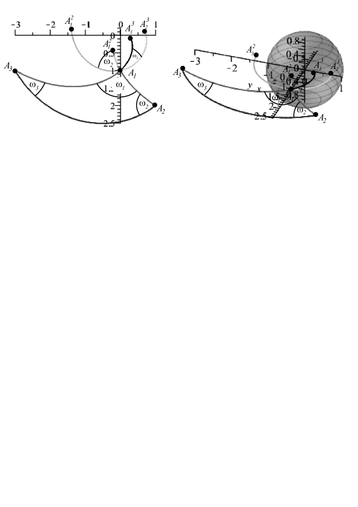
Figure 9: Geodesic triangle with vertices $A_{1}=(1,1,0,0)$, $A_{2}=(1,2,3/2,1)$, $A_{3}=(1,3,-1,0)$ in $\mathbf{H}^{2}\!\times\!\mathbf{R}$ geometry, and transformed images of its geodesic side segments. The geodesic curve segments $g{(A_{1},A_{2})}$, $g{(A_{2},A_{3})}$, $g({A_{3},A_{1}})$ lie on the coordinate plane $[x,y]$ and the interior angle sum of this geodesic triangle is $\sum_{i=1}^{3}(\omega_{i})=\pi$.

We can determine the interior angle sum of arbitrary $\mathbf{H}^{2}\!\times\!\mathbf{R}$ geodesic triangle. In the following table we summarize some numerical data of interior angles of given geodesic triangles:

Table 2:   $A_{1}=(1,0,0,0)$, $A_{2}=(1,2,3/2,1)$ $A_{3}$ $\omega_{1}$ $\omega_{2}$ $\omega_{3}$ $\sum_{i=1}^{3}(\omega_{i})$ $(1,3/\sqrt{8},-1/\sqrt{8},0)$ $2.54659$ $0.06953$ $0.41780$ $3.03392$ $(1,3,-1,0)$ $1.93230$ $0.49280$ $0.69816$ $3.12325$ $(1,6,-2,0)$ $1.83102$ $0.71611$ $0.58348$ $3.13061$ $(1,9,-3,0)$ $1.80083$ $0.81224$ $0.51964$ $3.13270$ $(1,3000,-1000,0)$ $1.70394$ $1.25735$ $0.17793$ $3.13922$

By the above experiences and computations we obtain the following

Theorem 3.9

If the Euclidean plane of the vertices of a $\mathbf{H}^{2}\!\times\!\mathbf{R}$ geodesic triangle $A_{1}A_{2}A_{3}$ does not contain the centre of model $E_{0}$ then its interior angle sum is less than $\pi$.

Proof: The proof is similar to the $\mathbf{S}^{2}\!\times\!\mathbf{R}$ case.

We can assume without loss of generality that the vertices $A_{1},A_{2}$ of such a geodesic triangle lie in the $[x,y]$ plane of the model. Using the Lemma 3.7 we get, that the geodesic segment $A_{i}A_{j}$, ($(i,j)\in\{(1,2),(1,3),2,3)\}$) is contained by the $A_{i}A_{j}E_{0}$ plane, therefore the sides of triangle $A_{1}A_{2}A_{3}$ lie in the boundary of trihedron given by the points $E_{0}$, $A_{1}$, $A_{2}$, $A_{3}$. It is clear, that all types of geodesic triangles can be described by such a triangle. Therefore, it is sufficient investigate the interior angle sums of geodesic triangles where we fix two of the vertices, e.g. $A_{1}$ and $A_{2}$ and move the third vertex $A_{3}$ on the half straight line $E_{0}A_{3}$ with starting point $E_{0}\neq A_{3}(t)$.

Remark 3.4

It is well known, that if the vertices $A_{1},A_{2},A_{3}$ lie in a ”upper” sheet of the two-sheeted hyperboloid (in the hyperboloid model of the hyperbolic plane geometry where the straight lines of hyperbolic 2-space are modeled by geodesics on the hyperboloid) centred at $E_{0}$ then the interior angle sum of hyperbolic triangle $A_{1}A_{2}A_{3}$ is less than $\pi$.

Let $\Delta(t)$ $(t\in\mathbf{R}^{+})$ denote the above geodesic triangle with interior angles at the vertex $A_{i}$ by $\omega_{i}(t)$ $(i\in\{1,2,3\})$.

The interior angle sum function $S(\Delta^{\mathbf{H}^{2}\!\times\!\mathbf{R}}(t))=\sum_{i=1}^{3}(\omega_{i}(t))$ can be determined related to the parameters $x_{2},y_{2},z_{2},x_{3},y_{3}\in\mathbf{R}$ by the formulas (2.10), (3.14), (3.15) and by the Lemma 3.6. Analyzing the above complicated continuous functions of single real variable $t$ we get that its maximum is achieved at a point $t_{0}\in(0,\infty)$ depending on given parameters. Moreover, $S(\Delta^{\mathbf{H}^{2}\!\times\!\mathbf{R}}(t))$ is stricly increasing on the interval $(0,t_{0})$, stricly decreasing on the interval $(t_{0},\infty)$ and

$$\lim_{t\rightarrow 0}S(\Delta^{\mathbf{H}^{2}\!\times\!\mathbf{R}}(t))=\pi,\leavevmode\nobreak\ \leavevmode\nobreak\ \leavevmode\nobreak\ \leavevmode\nobreak\ \lim_{t\rightarrow\infty}S(\Delta^{\mathbf{H}^{2}\!\times\!\mathbf{R}}(t))=\pi.\hskip 28.45274pt$$

Figure 10: $S(\Delta^{\mathbf{H}^{2}\!\times\!\mathbf{R}}(t))$ function related to parameters $x_{2}=2,y_{2}=3/1,z_{2}=1$ $x_{3}=3\cdot t,y_{3}=-1\cdot t,z_{3}=0$.

In Fig. 10 we described the $S(\Delta(t))$ function related to geodesic triangle $\Delta(t)$ $(t\in(0,5))$ with vertices $A_{1}=(1,1,0,0)$, $A_{2}=(1,2,3/2,1)$, $A_{3}=(1,3\cdot t,-1\cdot t,0)$. Its minimum is achieved at $t_{0}\approx 0.36392$ where $S(\Delta^{\mathbf{H}^{2}\!\times\!\mathbf{R}}(t_{0}))\approx 3.03236$.       $\square$

Finally we obtain the following

Theorem 3.10

The sum of the interior angles of a geodesic triangle of $\mathbf{H}^{2}\!\times\!\mathbf{R}$ space is less or equal to $\pi$.     $\square$