1 Introduction
Contact mechanics is an important and widely developed part of continuum
mechanics of solids, intensively studied during past decades from the
modelling, computational, and analytical aspects, too [58 , 60 , 59 , 66 , 68 ] . We focus on
a class of models for contacts with adhesion (cohesion) and friction in the
thermodynamical context. Our goal is to formulate a rather general
multi-purpose model unifying a relatively
wide menagerie of such particular
adhesion-friction models and to discuss its thermodynamics, outline
its conceptually efficient discretisation amenable for
calculation of vibrations/waves.
It is certainly impossible to present in a comprehensive way the relevant
literature to the part of contact mechanics covered by the general model
developed in the present paper. Anyhow, from the engineering point of view,
a detailed analysis of related variational formulations of
interface
cohesive models was developed in [21 ] . Another related and
thermodynamically based approach for general imperfect interfaces was proposed
and numerically studied in [24 , 30 , 29 ] ,
considering e.g. an interface temperature different from the temperatures of
adjacent bulks, cf. also [13 , 14 , 15 ]
for analytical considerations. Nevertheless, except [15 ] ,
friction dissipation was not
taken into account in these works. Coupling of cohesive models and friction
contact was developed after the pioneering work [62 ] , which assumed
the friction is activated after complete cohesive failure, in a series of
relevant contributions [2 , 9 , 19 , 22 , 27 , 36 , 37 , 41 , 42 , 53 , 57 , 61 , 64 ] among others, providing, for isothermal
configurations, a continuous transition from the cohesive state to the frictional contact state.
However, no rigorous proof of the solution existence or the convergence of a numerical scheme to the exact solution was provided in these works.
From the mathematical point of view, overviews of existing partial models in
literature can be found, e.g., without Coulomb friction (𝔣 = 0 𝔣 0 \mathfrak{f}=0 [20 , 49 , 52 ] (isothermal), without
inertia/friction and
interfacial plasticity but with fracture-mode-mixity sensitive debonding
(sometimes called also delamination) in [31 ] (isothermal)
or [43 , 44 ] (anisothermal); see also a review chapter [50 ] .
Models of adhesive contacts are to a great extent inspired
by bulk damage possibly combined with plasticity. The role of a scalar
damage variable is then replaced by an
interface damage (a concept invented by M. Frémond
[25 , 26 ] , also
called debonding or delamination, the term adopted hereinafter)
variable and plasticity can be transferred to a plastic slip,
cf. Remark 2.4 Like in the bulk models,
there are many options:
(i)
delamination can influence the elasticity
of the adhesive (through decaying elastic moduli) or
the plasticity (through decaying plastic yield stress for the plastic slip),
or both;
(ii)
vice versa, plasticity can influence delamination
indirectly through influencing the stress and displacement jump,
or directly through influencing activation threshold for delamination;
(iii)
delamination evolution can be either unidirectional
or reversible (i.e. admitting a so-called healing);
(iv)
delamination and interfacial plasticity can be considered
rate-independent
(and then choosing an appropriate concept of solution becomes a vital part
of the model itself and should carefully be considered, cf. [38 ] )
or rate-dependent (visco-plasticity, viscous delamination),
i.e. 4 options altogether, or more if also healing is
involved either as rate-dependent or rate-independent;
(v)
interfacial plasticity can be either with hardening
or without hardening;
(vi)
length scale (gradients) can be considered in interfacial
damage or/and plasticity.
In contrast to the mentioned bulk models, the interfacial analog
can additionally be combined with friction. We can then identify
other options (beside the trivial option just ignoring friction):
(vii)
friction acts on the displacement velocity, or can be realized
through the interfacial plastic slip;
(viii)
the contact is unilateral or bilateral, in the former case
the adhesion being mode sensitive or insensitive, possibly in
the normal-compliance variant counting with a small penetration
(microscopically related to various
asperities, cf. e.g. [63 ] for a detailed discussion).
Of course, as a general feature in (contact) mechanics, there is still
an option as far as temperature variation and related heat transfer concerns:
(ix)
either to ignore it by considering the model isothermal, or
to consider heat transfer in the bulk and through the contact
interface
but ignoring the heat capacity and the heat transfer in the adhesive
itself, or even to involve this latter heat problem in the adhesive, too.
In addition, various non-linearities can be considered at various
parts of the models, leading e.g. to various cohesive-contact models etc.
Eventually, there are standard options as far as the bulk models:
purely elastic or visco-elastic with various rheologies (possibly involving
creep) or some additional inelastic processes like plasticity,
purely quasistatic models versus inertial effects involved,
simple or nonsimple materials, cf. [44 ] , linear or nonlinear
materials, purely isothermal versus anisothermal with or without thermal
expansion, etc.
Contact mechanics has many applications in engineering or in (for example geo-)
physics, and various combinations of the above identified options (i)–(ix)
may serve for various purposes. Of course, not all combinations give sensible
models or are amenable for a rigorous analysis supporting
also executable numerical schemes with guaranteed stability and convergence.
The above outlined rich menagerie of inelastic-contact models however should not
create a false impression that it covers everything. In particular, in this
paper we ignore phenomena like fatigue or wear, and we
confine ourselves to small strains and, in addition, we also assume small
displacements (and thus a prescribed contact zone, avoiding e.g. contact
of rolling bodies or a varying Hertz’ contact zone).
Moreover, there is also a lot of contact-mechanical models based on
hemivariational inequalities involving nonsmooth nonconvex functions,
cf. e.g. [8 , 4 , 39 ] . Often, this
mathematically involved and numerically more difficult setting results
rather from lacking of suitable internal variables. In contrast, the
definite advantage of our general model is that it relies on classical
variational inequalities involving convex functions only.
The plan of this paper is the following: In Section 2 coupling the adhesive layer with
the viscoelastic bulk. Then, in Section 3 devise its “monolithic” formulation treating the bulk and
the adhesive in a unified way, and discuss its energetics and thermodynamical
consistency. Then, in Section 4 energy-conserving time
discretisation allowing for efficient computer implementation is devised
and its numerical stability and convergence is outlined. Eventually,
in Section 5
For readers’ convenience, let us summarize
the basic notation used in what follows in Table 1
Ω , Ω 1 , Ω 2 ⊂ ℝ d Ω subscript Ω 1 subscript Ω 2
superscript ℝ 𝑑 \varOmega,\varOmega_{1},\varOmega_{2}\subset{\mathbb{R}}^{d} domains,
Ω 1 ∩ Ω 2 = ∅ subscript Ω 1 subscript Ω 2 \ \varOmega_{1}{\cap}\varOmega_{2}=\emptyset d = 2 , 3 𝑑 2 3
d=2,3 dimension of the problem, Γ C subscript Γ C \mathchoice{\varGamma_{\mbox{\tiny\rm C}}}{\varGamma_{\mbox{\tiny\rm C}}}{\varGamma_{\mbox{\tiny\rm C}}}{\varGamma_{\mbox{\tiny\rm C}}} contact interface,
Ω ∖ Γ C = Ω 1 ∪ Ω 2 Ω subscript Γ C subscript Ω 1 subscript Ω 2 \ \varOmega\!\setminus\!\mathchoice{\varGamma_{\mbox{\tiny\rm C}}}{\varGamma_{\mbox{\tiny\rm C}}}{\varGamma_{\mbox{\tiny\rm C}}}{\varGamma_{\mbox{\tiny\rm C}}}=\varOmega_{1}{\cup}\varOmega_{2} ℝ sym d × d := { A ∈ ℝ d × d ; A = A ⊤ } assign superscript subscript ℝ sym 𝑑 𝑑 formulae-sequence 𝐴 superscript ℝ 𝑑 𝑑 𝐴 superscript 𝐴 top {\mathbb{R}}_{\mathrm{sym}}^{d\times d}:=\{A\!\in\!{\mathbb{R}}^{d\times d};\ A=A^{\top}\} , u : Q ∖ Σ C → ℝ d : 𝑢 → 𝑄 subscript Σ C superscript ℝ 𝑑 u:Q{\setminus}\Sigma_{\mbox{\tiny\rm C}}\to{\mathbb{R}}^{d} displacement, π : Σ C → ℝ d − 1 : 𝜋 → subscript Σ C superscript ℝ 𝑑 1 \pi{:}\Sigma_{\mbox{\tiny\rm C}}\to{\mathbb{R}}^{d-1} plastic-like interfacial slip, α : Σ C → [ 0 , 1 ] : 𝛼 → subscript Σ C 0 1 \alpha:\Sigma_{\mbox{\tiny\rm C}}\to[0,1] interfacial damage, (delamination) variable, θ A : Σ C → ℝ + : subscript 𝜃 A → subscript Σ C superscript ℝ \theta_{\scriptscriptstyle\textrm{A}}\!:\Sigma_{\mbox{\tiny\rm C}}\to{\mathbb{R}}^{+}
temperature in the adhesive, θ B : Q ∖ Σ C → ℝ + : subscript 𝜃 B → 𝑄 subscript Σ C superscript ℝ \theta_{\scriptscriptstyle\textrm{B}}:Q{\setminus}\Sigma_{\mbox{\tiny\rm C}}{\to}{\mathbb{R}}^{+}
bulk temperature, e ( u ) = 1 2 ∇ u ⊤ + 1 2 ∇ u 𝑒 𝑢 1 2 ∇ superscript 𝑢 top 1 2 ∇ 𝑢 e(u)=\frac{1}{2}\nabla u^{\top}\!+\frac{1}{2}\nabla u
small-strain tensor,
[ [ u ] ] : Σ C → ℝ d : delimited-[] delimited-[] 𝑢 → subscript Σ C superscript ℝ 𝑑 \mathchoice{\big{[}\big{[}u\big{]}\big{]}}{[[u]]}{[\![u]\!]}{[\![u]\!]}:\Sigma_{\mbox{\tiny\rm C}}\to{\mathbb{R}}^{d} jump of u 𝑢 u Γ C subscript Γ C \mathchoice{\varGamma_{\mbox{\tiny\rm C}}}{\varGamma_{\mbox{\tiny\rm C}}}{\varGamma_{\mbox{\tiny\rm C}}}{\varGamma_{\mbox{\tiny\rm C}}} [ [ u ] ] N subscript delimited-[] delimited-[] 𝑢 N \mathchoice{\big{[}\big{[}u\big{]}\big{]}_{{{}_{\rm N}}}}{[[u]]_{{{}_{\rm N}}}}{[\![u]\!]_{{{}_{\rm N}}}}{[\![u]\!]_{{{}_{\rm N}}}} normal jump of u 𝑢 u Γ C subscript Γ C \mathchoice{\varGamma_{\mbox{\tiny\rm C}}}{\varGamma_{\mbox{\tiny\rm C}}}{\varGamma_{\mbox{\tiny\rm C}}}{\varGamma_{\mbox{\tiny\rm C}}} [ [ u ] ] T subscript delimited-[] delimited-[] 𝑢 T \mathchoice{\big{[}\big{[}u\big{]}\big{]}_{{{}_{\rm T}}}}{[[u]]_{{{}_{\rm T}}}}{[\![u]\!]_{{{}_{\rm T}}}}{[\![u]\!]_{{{}_{\rm T}}}} tangential jump of u 𝑢 u Γ C subscript Γ C \mathchoice{\varGamma_{\mbox{\tiny\rm C}}}{\varGamma_{\mbox{\tiny\rm C}}}{\varGamma_{\mbox{\tiny\rm C}}}{\varGamma_{\mbox{\tiny\rm C}}} 𝑬 : u ↦ ( e ( u ) , [ [ u ] ] ) : 𝑬 maps-to 𝑢 𝑒 𝑢 delimited-[] delimited-[] 𝑢 \boldsymbol{E}:u\mapsto(e(u),\mathchoice{\big{[}\big{[}u\big{]}\big{]}}{[[u]]}{[\![u]\!]}{[\![u]\!]}) , η A : Σ C → ℝ : subscript 𝜂 A → subscript Σ C ℝ \eta_{\scriptscriptstyle\textrm{A}}\!:\Sigma_{\mbox{\tiny\rm C}}\to{\mathbb{R}}
entropy in the adhesive, η B : Q ∖ Σ C → ℝ : subscript 𝜂 B → 𝑄 subscript Σ C ℝ \eta_{\scriptscriptstyle\textrm{B}}:Q{\setminus}\Sigma_{\mbox{\tiny\rm C}}\to{\mathbb{R}} specific bulk entropy, ϑ A subscript italic-ϑ A \vartheta_{\scriptscriptstyle\textrm{\hskip 0.225ptA}} heat part of internal energy in the adhesive, ϑ B subscript italic-ϑ B \vartheta_{\scriptscriptstyle\textrm{\hskip 0.225ptB}} heat part of the bulk internal energy, f : Σ N → ℝ d : 𝑓 → subscript Σ N superscript ℝ 𝑑 f:\Sigma_{\mbox{\tiny\rm N}}\to{\mathbb{R}}^{d} applied traction force, g : Q → ℝ d : 𝑔 → 𝑄 superscript ℝ 𝑑 g:Q\to{\mathbb{R}}^{d} applied bulk force (gravity), σ 𝜎 \sigma stress in the bulk, ζ A subscript 𝜁 A \zeta_{\scriptscriptstyle\textrm{A}} the content of diffusant in the adhesive, ζ B subscript 𝜁 B \zeta_{\scriptscriptstyle\textrm{B}} the content of diffusant in the bulk, ℂ ∈ ℝ d 4 ℂ superscript ℝ superscript 𝑑 4 \mathbb{C}\in{\mathbb{R}}^{d^{4}} elasticity tensor, 𝔻 ∈ ℝ d 4 𝔻 superscript ℝ superscript 𝑑 4 \mathbb{D}\in{\mathbb{R}}^{d^{4}} viscosity tensor, 𝕂 A ∈ ℝ ( d − 1 ) × ( d − 1 ) subscript 𝕂 A superscript ℝ 𝑑 1 𝑑 1 \mathbb{K}_{\scriptscriptstyle\textrm{\hskip 0.225ptA}}\in{\mathbb{R}}^{{\color[rgb]{0,0,0}(d{-}1)\times(d{-}1)}}
adhesive heat conductivity, 𝕂 B = 𝕂 B ( θ B ) ∈ ℝ d × d subscript 𝕂 B subscript 𝕂 B subscript 𝜃 B superscript ℝ 𝑑 𝑑 \mathbb{K}_{\scriptscriptstyle\textrm{\hskip 0.225ptB}}=\mathbb{K}_{\scriptscriptstyle\textrm{\hskip 0.225ptB}}(\theta_{\scriptscriptstyle\textrm{B}})\in{\mathbb{R}}^{{\color[rgb]{0,0,0}d\times d}} bulk heat conductivity,
𝔼 ∈ ℝ d × d 𝔼 superscript ℝ 𝑑 𝑑 \mathbb{E}\in{\mathbb{R}}^{d\times d} thermal-expansion tensor, ϱ italic-ϱ \varrho mass density, 𝕄 A subscript 𝕄 A {\mathbb{M}}_{\scriptscriptstyle\textrm{A}} , 𝕄 B subscript 𝕄 B {\mathbb{M}}_{\scriptscriptstyle\textrm{B}} , m 𝑚 m mobility between the adhesive and the bulk, M A , M B subscript 𝑀 A subscript 𝑀 B
M_{\scriptscriptstyle\textrm{A}},\,M_{\scriptscriptstyle\textrm{B}} Biot moduli in the adhesive and bulk, β A , β B subscript 𝛽 A subscript 𝛽 B
\beta_{\scriptscriptstyle\textrm{A}},\,\beta_{\scriptscriptstyle\textrm{B}} Biot coefficients in the adhesive and bulk, μ A , μ B subscript 𝜇 A subscript 𝜇 B
\mu_{\scriptscriptstyle\textrm{A}},\mu_{\scriptscriptstyle\textrm{B}} chemical potentials in the adhesive and bulk, σ C subscript 𝜎 C \sigma_{{}_{\rm C}} , σ F subscript 𝜎 F \sigma_{{}_{\rm F}} σ T , subscript 𝜎 T \sigma_{{}_{\rm T}}, σ N subscript 𝜎 N \sigma_{{}_{\rm N}} c B = c B ( θ B ) subscript 𝑐 B subscript 𝑐 B subscript 𝜃 B c_{\scriptscriptstyle\textrm{\hskip 0.225ptB}}=c_{\scriptscriptstyle\textrm{\hskip 0.225ptB}}(\theta_{\scriptscriptstyle\textrm{B}}) bulk heat capacity, c A = c A ( θ A ) subscript 𝑐 A subscript 𝑐 A subscript 𝜃 A c_{\scriptscriptstyle\textrm{\hskip 0.225ptA}}=c_{\scriptscriptstyle\textrm{\hskip 0.225ptA}}(\theta_{\scriptscriptstyle\textrm{A}}) adhesive heat capacity, 𝐤 A ( [ [ u ] ] N , α , θ A ) subscript 𝐤 A subscript delimited-[] delimited-[] 𝑢 N 𝛼 subscript 𝜃 A \mathbf{k}_{\scriptscriptstyle\textrm{\hskip 0.225ptA}}({\color[rgb]{0,0,0}\mathchoice{\big{[}\big{[}u\big{]}\big{]}_{{{}_{\rm N}}}}{[[u]]_{{{}_{\rm N}}}}{[\![u]\!]_{{{}_{\rm N}}}}{[\![u]\!]_{{{}_{\rm N}}}}},\alpha,\theta_{\scriptscriptstyle\textrm{A}}) bulk-to-adhesive
heat
coefficients,
u D : Σ D → ℝ d : subscript 𝑢 D → subscript Σ D superscript ℝ 𝑑 u_{\mbox{\tiny\rm D}}:\Sigma_{\mbox{\tiny\rm D}}\to{\mathbb{R}}^{d} prescribed
boundary displacement, 𝔣 ( α , θ A ) 𝔣 𝛼 subscript 𝜃 A \mathfrak{f}(\alpha,\theta_{\scriptscriptstyle\textrm{A}}) friction coefficient, σ y ( α , θ A ) subscript 𝜎 y 𝛼 subscript 𝜃 A \sigma_{\rm y}(\alpha,\theta_{\scriptscriptstyle\textrm{A}}) yield-stress for plastic slip, a 1 ( [ [ u ] ] , α , θ A , α . ) subscript 𝑎 1 delimited-[] delimited-[] 𝑢 𝛼 subscript 𝜃 A superscript 𝛼 . a_{1}({\color[rgb]{0,0,0}\mathchoice{\big{[}\big{[}u\big{]}\big{]}}{[[u]]}{[\![u]\!]}{[\![u]\!]}},\alpha,\theta_{\scriptscriptstyle\textrm{A}},\mathchoice{{\buildrel\hskip 0.90005pt\text{\LARGE.}\over{\alpha}}}{{\buildrel\hskip 0.90005pt\text{\Large.}\over{\alpha}}}{{\buildrel\hskip 0.90005pt\text{\large.}\over{\alpha}}}{{\buildrel\hskip 0.90005pt\text{\large.}\over{\alpha}}}) delamination dissipation
potential, a 0 ( α ) + b 0 ( α ) θ A subscript 𝑎 0 𝛼 subscript 𝑏 0 𝛼 subscript 𝜃 A a_{0}(\alpha)+b_{0}(\alpha)\theta_{\scriptscriptstyle\textrm{A}} stored energy of delamination, γ T ( α , ⋅ ) subscript 𝛾 T 𝛼 ⋅ \gamma_{{}_{\rm T}}(\alpha,\cdot) , γ N ( α , ⋅ ) subscript 𝛾 N 𝛼 ⋅ \gamma_{{}_{\rm N}}(\alpha,\cdot) γ C ( [ [ u ] ] ) subscript 𝛾 C delimited-[] delimited-[] 𝑢 \gamma_{\scriptscriptstyle\textrm{C}}({\color[rgb]{0,0,0}\mathchoice{\big{[}\big{[}u\big{]}\big{]}}{[[u]]}{[\![u]\!]}{[\![u]\!]}}) normal-compliance potential, d N = d N ( α , θ A ) subscript 𝑑 N subscript 𝑑 N 𝛼 subscript 𝜃 A d_{{}_{\rm N}}=d_{{}_{\rm N}}(\alpha,\theta_{\scriptscriptstyle\textrm{A}}) normal viscosity of adhesive, d T = d T ( α , θ A ) subscript 𝑑 T subscript 𝑑 T 𝛼 subscript 𝜃 A d_{{}_{\rm T}}=d_{{}_{\rm T}}(\alpha,\theta_{\scriptscriptstyle\textrm{A}}) tangential viscosity of adhesive, κ H ≥ 0 subscript 𝜅 H 0 \kappa_{\rm H}\geq 0 hardening coefficient for plastic slip, κ 1 > 0 subscript 𝜅 1 0 \kappa_{1}>0 scale coefficient of the gradient of π 𝜋 \pi κ 2 > 0 subscript 𝜅 2 0 \kappa_{2}>0 scale coefficient of the gradient of α 𝛼 \alpha Ψ Ψ \varPsi total free energy, Ξ Ξ \varXi total potential of dissipative forces, R 𝑅 R total dissipation rate, M 𝑀 M total kinetic energy.
Table 1: Summary of the basic notation used through the paper.
For the notation Q 𝑄 Q Σ C subscript Σ C \Sigma_{\mbox{\tiny\rm C}} Σ D subscript Σ D \Sigma_{\mbox{\tiny\rm D}} 2.2 1
2 The general model
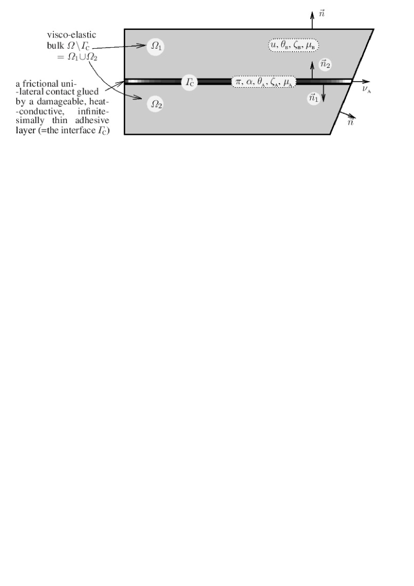
We consider a bounded Lipschitz domain Ω ⊂ ℝ d Ω superscript ℝ 𝑑 \varOmega\subset{\mathbb{R}}^{d} Γ C subscript Γ C \mathchoice{\varGamma_{\mbox{\tiny\rm C}}}{\varGamma_{\mbox{\tiny\rm C}}}{\varGamma_{\mbox{\tiny\rm C}}}{\varGamma_{\mbox{\tiny\rm C}}} 1 θ A subscript 𝜃 A \theta_{\scriptscriptstyle\textrm{A}} ( d − 1 ) 𝑑 1 (d{-}1) interface Γ C subscript Γ C \mathchoice{\varGamma_{\mbox{\tiny\rm C}}}{\varGamma_{\mbox{\tiny\rm C}}}{\varGamma_{\mbox{\tiny\rm C}}}{\varGamma_{\mbox{\tiny\rm C}}} d 𝑑 d [13 , 14 , 16 ] or
[38 , Sect.5.3.3.3] for such a model,
or in combination with a friction also [15 ] .
For a relation to models which avoid this interface-temperature
concept see Remark 2.2
Figure 1: Schematic geometry of one contact interface Γ C subscript Γ C \mathchoice{\varGamma_{\mbox{\tiny\rm C}}}{\varGamma_{\mbox{\tiny\rm C}}}{\varGamma_{\mbox{\tiny\rm C}}}{\varGamma_{\mbox{\tiny\rm C}}} Ω Ω \varOmega the adhesive on Γ C subscript Γ C \mathchoice{\varGamma_{\mbox{\tiny\rm C}}}{\varGamma_{\mbox{\tiny\rm C}}}{\varGamma_{\mbox{\tiny\rm C}}}{\varGamma_{\mbox{\tiny\rm C}}}
The unit normal vector to Ω i subscript Ω 𝑖 \varOmega_{i} ( i = 1 , 2 ) 𝑖 1 2
(i=1,2) n → i subscript → 𝑛 𝑖 \vec{n}_{i} n → 1 = − n → 2 subscript → 𝑛 1 subscript → 𝑛 2 \vec{n}_{1}=-\vec{n}_{2} Γ C subscript Γ C \mathchoice{\varGamma_{\mbox{\tiny\rm C}}}{\varGamma_{\mbox{\tiny\rm C}}}{\varGamma_{\mbox{\tiny\rm C}}}{\varGamma_{\mbox{\tiny\rm C}}} n → = n → i → 𝑛 subscript → 𝑛 𝑖 \vec{n}=\vec{n}_{i} ∂ Ω i ∖ Γ C subscript Ω 𝑖 subscript Γ C \partial\varOmega_{i}{\setminus}\mathchoice{\varGamma_{\mbox{\tiny\rm C}}}{\varGamma_{\mbox{\tiny\rm C}}}{\varGamma_{\mbox{\tiny\rm C}}}{\varGamma_{\mbox{\tiny\rm C}}} 1 Γ C subscript Γ C \mathchoice{\varGamma_{\mbox{\tiny\rm C}}}{\varGamma_{\mbox{\tiny\rm C}}}{\varGamma_{\mbox{\tiny\rm C}}}{\varGamma_{\mbox{\tiny\rm C}}} Ω 1 subscript Ω 1 \varOmega_{1} Ω 2 subscript Ω 2 \varOmega_{2}
[ [ u ] ] := u 1 | Γ C − u 2 | Γ C , [ [ u ] ] N := [ [ u ] ] ⋅ n → 2 = ( u 2 | Γ C − u 1 | Γ C ) ⋅ n → 1 , [ [ u ] ] T := [ [ u ] ] − [ [ u ] ] N n → 2 . formulae-sequence formulae-sequence assign delimited-[] delimited-[] 𝑢 evaluated-at subscript 𝑢 1 subscript Γ C evaluated-at subscript 𝑢 2 subscript Γ C assign subscript delimited-[] delimited-[] 𝑢 N ⋅ delimited-[] delimited-[] 𝑢 subscript → 𝑛 2 ⋅ evaluated-at subscript 𝑢 2 subscript Γ C evaluated-at subscript 𝑢 1 subscript Γ C subscript → 𝑛 1 assign subscript delimited-[] delimited-[] 𝑢 T delimited-[] delimited-[] 𝑢 subscript delimited-[] delimited-[] 𝑢 N subscript → 𝑛 2 \displaystyle\mathchoice{\big{[}\big{[}u\big{]}\big{]}}{[[u]]}{[\![u]\!]}{[\![u]\!]}\!:=u_{1}|_{\mathchoice{\varGamma_{\mbox{\tiny\rm C}}}{\varGamma_{\mbox{\tiny\rm C}}}{\varGamma_{\mbox{\tiny\rm C}}}{\varGamma_{\mbox{\tiny\rm C}}}}\!-u_{2}|_{\mathchoice{\varGamma_{\mbox{\tiny\rm C}}}{\varGamma_{\mbox{\tiny\rm C}}}{\varGamma_{\mbox{\tiny\rm C}}}{\varGamma_{\mbox{\tiny\rm C}}}},\ \ \mathchoice{\big{[}\big{[}u\big{]}\big{]}_{{{}_{\rm N}}}}{[[u]]_{{{}_{\rm N}}}}{[\![u]\!]_{{{}_{\rm N}}}}{[\![u]\!]_{{{}_{\rm N}}}}\!\!:=\mathchoice{\big{[}\big{[}u\big{]}\big{]}}{[[u]]}{[\![u]\!]}{[\![u]\!]}{{\cdot}}\vec{n}_{2}=\big{(}u_{2}|_{\mathchoice{\varGamma_{\mbox{\tiny\rm C}}}{\varGamma_{\mbox{\tiny\rm C}}}{\varGamma_{\mbox{\tiny\rm C}}}{\varGamma_{\mbox{\tiny\rm C}}}}\!-u_{1}|_{\mathchoice{\varGamma_{\mbox{\tiny\rm C}}}{\varGamma_{\mbox{\tiny\rm C}}}{\varGamma_{\mbox{\tiny\rm C}}}{\varGamma_{\mbox{\tiny\rm C}}}}\big{)}{{\cdot}}\vec{n}_{1},\ \ \mathchoice{\big{[}\big{[}u\big{]}\big{]}_{{{}_{\rm T}}}}{[[u]]_{{{}_{\rm T}}}}{[\![u]\!]_{{{}_{\rm T}}}}{[\![u]\!]_{{{}_{\rm T}}}}\!\!:=\mathchoice{\big{[}\big{[}u\big{]}\big{]}}{[[u]]}{[\![u]\!]}{[\![u]\!]}\!-\mathchoice{\big{[}\big{[}u\big{]}\big{]}_{{{}_{\rm N}}}}{[[u]]_{{{}_{\rm N}}}}{[\![u]\!]_{{{}_{\rm N}}}}{[\![u]\!]_{{{}_{\rm N}}}}\vec{n}_{2}. (2.1)
Thus, e.g. [ [ u ] ] N > 0 subscript delimited-[] delimited-[] 𝑢 N 0 \mathchoice{\big{[}\big{[}u\big{]}\big{]}_{{{}_{\rm N}}}}{[[u]]_{{{}_{\rm N}}}}{[\![u]\!]_{{{}_{\rm N}}}}{[\![u]\!]_{{{}_{\rm N}}}}>0 Ω 1 subscript Ω 1 \varOmega_{1} Ω 2 subscript Ω 2 \varOmega_{2} Γ C subscript Γ C \mathchoice{\varGamma_{\mbox{\tiny\rm C}}}{\varGamma_{\mbox{\tiny\rm C}}}{\varGamma_{\mbox{\tiny\rm C}}}{\varGamma_{\mbox{\tiny\rm C}}} [ [ u ] ] N < 0 subscript delimited-[] delimited-[] 𝑢 N 0 \mathchoice{\big{[}\big{[}u\big{]}\big{]}_{{{}_{\rm N}}}}{[[u]]_{{{}_{\rm N}}}}{[\![u]\!]_{{{}_{\rm N}}}}{[\![u]\!]_{{{}_{\rm N}}}}<0
We further consider the boundary of Ω Ω \varOmega Γ D subscript Γ D \varGamma_{\mbox{\tiny\rm D}} Γ N subscript Γ N \varGamma_{\mbox{\tiny\rm N}} T > 0 𝑇 0 T>0
Q := ( 0 , T ) × Ω , Σ := ( 0 , T ) × ∂ Ω , formulae-sequence assign 𝑄 0 𝑇 Ω assign Σ 0 𝑇 Ω \displaystyle Q:=(0,T)\times\varOmega,\qquad\Sigma:=(0,T)\times\partial\varOmega,\quad (2.2a)
Σ C := ( 0 , T ) × Γ C , Σ D := ( 0 , T ) × Γ D , Σ N := ( 0 , T ) × Γ N . formulae-sequence assign subscript Σ C 0 𝑇 subscript Γ C formulae-sequence assign subscript Σ D 0 𝑇 subscript Γ D assign subscript Σ N 0 𝑇 subscript Γ N \displaystyle\Sigma_{\mbox{\tiny\rm C}}:=(0,T)\times\mathchoice{\varGamma_{\mbox{\tiny\rm C}}}{\varGamma_{\mbox{\tiny\rm C}}}{\varGamma_{\mbox{\tiny\rm C}}}{\varGamma_{\mbox{\tiny\rm C}}},\quad\ \Sigma_{\mbox{\tiny\rm D}}:=(0,T)\times\varGamma_{\mbox{\tiny\rm D}},\quad\ \Sigma_{\mbox{\tiny\rm N}}:=(0,T)\times\varGamma_{\mbox{\tiny\rm N}}. (2.2b)
One of the main ingredient of the model will be
the force
balance on the contact interface Γ C subscript Γ C \mathchoice{\varGamma_{\mbox{\tiny\rm C}}}{\varGamma_{\mbox{\tiny\rm C}}}{\varGamma_{\mbox{\tiny\rm C}}}{\varGamma_{\mbox{\tiny\rm C}}}
[ [ σ ] ] n → = 0 with σ := 𝔻 e ( u . ) + ℂ ( e ( u ) − 𝔼 θ B + 𝔼 θ R ) formulae-sequence delimited-[] delimited-[] 𝜎 → 𝑛 0 assign with 𝜎 𝔻 𝑒 superscript 𝑢 . ℂ 𝑒 𝑢 𝔼 subscript 𝜃 B 𝔼 subscript 𝜃 R \displaystyle\mathchoice{\big{[}\big{[}\sigma\big{]}\big{]}}{[[\sigma]]}{[\![\sigma]\!]}{[\![\sigma]\!]}\vec{n}=0\ \ \ \ \ \text{ with }\ \sigma:=\mathbb{D}e(\mathchoice{{\buildrel\hskip 1.00006pt\text{\LARGE.}\over{u}}}{{\buildrel\hskip 1.00006pt\text{\Large.}\over{u}}}{{\buildrel\hskip 1.00006pt\text{\large.}\over{u}}}{{\buildrel\hskip 1.00006pt\text{\large.}\over{u}}})+\mathbb{C}(e(u){-}\mathbb{E}\theta_{\scriptscriptstyle\textrm{B}}{\color[rgb]{0,0,0}{{+}\mathbb{E}\theta_{{}_{\rm R}}}}) on Σ C , on subscript Σ C \displaystyle\text{on }\Sigma_{\mbox{\tiny\rm C}},\hskip 11.99998pt (2.3a)
| σ F | ≤ − 𝔣 σ C with 𝔣 = 𝔣 ( α , θ A ) , σ C := γ C ′ ( [ [ u ] ] N ) , formulae-sequence subscript 𝜎 F 𝔣 subscript 𝜎 C formulae-sequence with 𝔣 𝔣 𝛼 subscript 𝜃 A assign subscript 𝜎 C superscript subscript 𝛾 C ′ subscript delimited-[] delimited-[] 𝑢 N \displaystyle|\sigma_{{}_{\rm F}}|\leq-\mathfrak{f}\sigma_{{}_{\rm C}}\ \ \text{ with }\ \mathfrak{f}=\mathfrak{f}(\alpha,\theta_{\scriptscriptstyle\textrm{A}}),\ \ \ \sigma_{{}_{\rm C}}:=\gamma_{\scriptscriptstyle\textrm{C}}^{\prime}({\mathchoice{\big{[}\big{[}u\big{]}\big{]}}{[[u]]}{[\![u]\!]}{[\![u]\!]}}_{{}_{\rm N}}),
and σ F := σ T − [ γ T ] v ′ ( α , [ [ u ] ] T − π ) − d T ( α , θ A ) ( [ [ u . ] ] T − π . ) , \displaystyle\hskip 60.00009pt\text{ and }\ \ \sigma_{{}_{\rm F}}:=\sigma_{{}_{\rm T}}-\big{[}\gamma_{{}_{\rm T}}\big{]}_{v}^{\prime}\big{(}\alpha,\mathchoice{\big{[}\big{[}u\big{]}\big{]}_{{{}_{\rm T}}}}{[[u]]_{{{}_{\rm T}}}}{[\![u]\!]_{{{}_{\rm T}}}}{[\![u]\!]_{{{}_{\rm T}}}}\!{-}\pi\big{)}-d_{{}_{\rm T}}(\alpha,\theta_{\scriptscriptstyle\textrm{A}})\big{(}\mathchoice{\big{[}\big{[}\mathchoice{{\buildrel\hskip 1.00006pt\text{\LARGE.}\over{u}}}{{\buildrel\hskip 1.00006pt\text{\Large.}\over{u}}}{{\buildrel\hskip 1.00006pt\text{\large.}\over{u}}}{{\buildrel\hskip 1.00006pt\text{\large.}\over{u}}}\big{]}\big{]}_{{{}_{\rm T}}}}{[[\mathchoice{{\buildrel\hskip 1.00006pt\text{\LARGE.}\over{u}}}{{\buildrel\hskip 1.00006pt\text{\Large.}\over{u}}}{{\buildrel\hskip 1.00006pt\text{\large.}\over{u}}}{{\buildrel\hskip 1.00006pt\text{\large.}\over{u}}}]]_{{{}_{\rm T}}}}{[\![\mathchoice{{\buildrel\hskip 1.00006pt\text{\LARGE.}\over{u}}}{{\buildrel\hskip 1.00006pt\text{\Large.}\over{u}}}{{\buildrel\hskip 1.00006pt\text{\large.}\over{u}}}{{\buildrel\hskip 1.00006pt\text{\large.}\over{u}}}]\!]_{{{}_{\rm T}}}}{[\![\mathchoice{{\buildrel\hskip 1.00006pt\text{\LARGE.}\over{u}}}{{\buildrel\hskip 1.00006pt\text{\Large.}\over{u}}}{{\buildrel\hskip 1.00006pt\text{\large.}\over{u}}}{{\buildrel\hskip 1.00006pt\text{\large.}\over{u}}}]\!]_{{{}_{\rm T}}}}\!{-}\mathchoice{{\buildrel\hskip 1.00006pt\text{\LARGE.}\over{\pi}}}{{\buildrel\hskip 1.00006pt\text{\Large.}\over{\pi}}}{{\buildrel\hskip 1.00006pt\text{\large.}\over{\pi}}}{{\buildrel\hskip 1.00006pt\text{\large.}\over{\pi}}}\big{)},
and σ T := σ n → 2 − σ N n → 2 with σ N := n → 2 ⊤ σ n → 2 formulae-sequence assign and subscript 𝜎 T
𝜎 subscript → 𝑛 2 subscript 𝜎 N subscript → 𝑛 2 assign with subscript 𝜎 N
superscript subscript → 𝑛 2 top 𝜎 subscript → 𝑛 2 \displaystyle\hskip 60.00009pt\text{ and }\ \ \sigma_{{}_{\rm T}}:=\sigma{\color[rgb]{0,0,0}{\vec{n}_{2}}}-\sigma_{{}_{\rm N}}{\color[rgb]{0,0,0}{\vec{n}_{2}}}\ \ \text{ with }\ \ \sigma_{{}_{\rm N}}:={\color[rgb]{0,0,0}{\vec{n}_{2}^{\top}}}\sigma{\color[rgb]{0,0,0}{\vec{n}_{2}}} on Σ C , on subscript Σ C \displaystyle\text{on }\Sigma_{\mbox{\tiny\rm C}},\hskip 11.99998pt (2.3b)
| σ F | < − 𝔣 σ C ⇒ [ [ u . ] ] T = 0 formulae-sequence subscript 𝜎 F 𝔣 subscript 𝜎 C ⇒
subscript delimited-[] delimited-[] superscript 𝑢 . T 0 \displaystyle|\sigma_{{}_{\rm F}}|<-\mathfrak{f}\sigma_{{}_{\rm C}}\ \ \ \Rightarrow\ \ \ \mathchoice{\big{[}\big{[}\mathchoice{{\buildrel\hskip 1.00006pt\text{\LARGE.}\over{u}}}{{\buildrel\hskip 1.00006pt\text{\Large.}\over{u}}}{{\buildrel\hskip 1.00006pt\text{\large.}\over{u}}}{{\buildrel\hskip 1.00006pt\text{\large.}\over{u}}}\big{]}\big{]}_{{{}_{\rm T}}}}{[[\mathchoice{{\buildrel\hskip 1.00006pt\text{\LARGE.}\over{u}}}{{\buildrel\hskip 1.00006pt\text{\Large.}\over{u}}}{{\buildrel\hskip 1.00006pt\text{\large.}\over{u}}}{{\buildrel\hskip 1.00006pt\text{\large.}\over{u}}}]]_{{{}_{\rm T}}}}{[\![\mathchoice{{\buildrel\hskip 1.00006pt\text{\LARGE.}\over{u}}}{{\buildrel\hskip 1.00006pt\text{\Large.}\over{u}}}{{\buildrel\hskip 1.00006pt\text{\large.}\over{u}}}{{\buildrel\hskip 1.00006pt\text{\large.}\over{u}}}]\!]_{{{}_{\rm T}}}}{[\![\mathchoice{{\buildrel\hskip 1.00006pt\text{\LARGE.}\over{u}}}{{\buildrel\hskip 1.00006pt\text{\Large.}\over{u}}}{{\buildrel\hskip 1.00006pt\text{\large.}\over{u}}}{{\buildrel\hskip 1.00006pt\text{\large.}\over{u}}}]\!]_{{{}_{\rm T}}}}=0 on Σ C , on subscript Σ C \displaystyle\text{on }\Sigma_{\mbox{\tiny\rm C}},\hskip 11.99998pt (2.3c)
| σ F | = − 𝔣 σ C ⇒ ∃ λ ≥ 0 : σ F = λ [ [ u . ] ] T \displaystyle|\sigma_{{}_{\rm F}}|=-\mathfrak{f}\sigma_{{}_{\rm C}}\ \ \ \Rightarrow\ \ \ \exists\lambda\geq 0:\ \ \sigma_{{}_{\rm F}}=\lambda\mathchoice{\big{[}\big{[}\mathchoice{{\buildrel\hskip 1.00006pt\text{\LARGE.}\over{u}}}{{\buildrel\hskip 1.00006pt\text{\Large.}\over{u}}}{{\buildrel\hskip 1.00006pt\text{\large.}\over{u}}}{{\buildrel\hskip 1.00006pt\text{\large.}\over{u}}}\big{]}\big{]}_{{{}_{\rm T}}}}{[[\mathchoice{{\buildrel\hskip 1.00006pt\text{\LARGE.}\over{u}}}{{\buildrel\hskip 1.00006pt\text{\Large.}\over{u}}}{{\buildrel\hskip 1.00006pt\text{\large.}\over{u}}}{{\buildrel\hskip 1.00006pt\text{\large.}\over{u}}}]]_{{{}_{\rm T}}}}{[\![\mathchoice{{\buildrel\hskip 1.00006pt\text{\LARGE.}\over{u}}}{{\buildrel\hskip 1.00006pt\text{\Large.}\over{u}}}{{\buildrel\hskip 1.00006pt\text{\large.}\over{u}}}{{\buildrel\hskip 1.00006pt\text{\large.}\over{u}}}]\!]_{{{}_{\rm T}}}}{[\![\mathchoice{{\buildrel\hskip 1.00006pt\text{\LARGE.}\over{u}}}{{\buildrel\hskip 1.00006pt\text{\Large.}\over{u}}}{{\buildrel\hskip 1.00006pt\text{\large.}\over{u}}}{{\buildrel\hskip 1.00006pt\text{\large.}\over{u}}}]\!]_{{{}_{\rm T}}}} on Σ C , on subscript Σ C \displaystyle\text{on }\Sigma_{\mbox{\tiny\rm C}},\hskip 11.99998pt (2.3d)
σ N − [ γ N ] v ′ ( α , [ [ u ] ] N ) − γ C ′ ( [ [ u ] ] N ) − d N ( α , θ A ) [ [ u . ] ] N = 0 subscript 𝜎 N superscript subscript delimited-[] subscript 𝛾 N 𝑣 ′ 𝛼 subscript delimited-[] delimited-[] 𝑢 N superscript subscript 𝛾 C ′ subscript delimited-[] delimited-[] 𝑢 N subscript 𝑑 N 𝛼 subscript 𝜃 A subscript delimited-[] delimited-[] superscript 𝑢 . N 0 \displaystyle\sigma_{{}_{\rm N}}-\big{[}\gamma_{{}_{\rm N}}\big{]}_{v}^{\prime}\big{(}{\alpha,}\mathchoice{\big{[}\big{[}u\big{]}\big{]}_{{{}_{\rm N}}}}{[[u]]_{{{}_{\rm N}}}}{[\![u]\!]_{{{}_{\rm N}}}}{[\![u]\!]_{{{}_{\rm N}}}}\big{)}-\gamma_{\scriptscriptstyle\textrm{C}}^{\prime}\big{(}{\mathchoice{\big{[}\big{[}u\big{]}\big{]}}{[[u]]}{[\![u]\!]}{[\![u]\!]}}_{{}_{\rm N}}\big{)}-d_{{}_{\rm N}}(\alpha,\theta_{\scriptscriptstyle\textrm{A}})\mathchoice{\big{[}\big{[}\mathchoice{{\buildrel\hskip 1.00006pt\text{\LARGE.}\over{u}}}{{\buildrel\hskip 1.00006pt\text{\Large.}\over{u}}}{{\buildrel\hskip 1.00006pt\text{\large.}\over{u}}}{{\buildrel\hskip 1.00006pt\text{\large.}\over{u}}}\big{]}\big{]}_{{{}_{\rm N}}}}{[[\mathchoice{{\buildrel\hskip 1.00006pt\text{\LARGE.}\over{u}}}{{\buildrel\hskip 1.00006pt\text{\Large.}\over{u}}}{{\buildrel\hskip 1.00006pt\text{\large.}\over{u}}}{{\buildrel\hskip 1.00006pt\text{\large.}\over{u}}}]]_{{{}_{\rm N}}}}{[\![\mathchoice{{\buildrel\hskip 1.00006pt\text{\LARGE.}\over{u}}}{{\buildrel\hskip 1.00006pt\text{\Large.}\over{u}}}{{\buildrel\hskip 1.00006pt\text{\large.}\over{u}}}{{\buildrel\hskip 1.00006pt\text{\large.}\over{u}}}]\!]_{{{}_{\rm N}}}}{[\![\mathchoice{{\buildrel\hskip 1.00006pt\text{\LARGE.}\over{u}}}{{\buildrel\hskip 1.00006pt\text{\Large.}\over{u}}}{{\buildrel\hskip 1.00006pt\text{\large.}\over{u}}}{{\buildrel\hskip 1.00006pt\text{\large.}\over{u}}}]\!]_{{{}_{\rm N}}}}=0 on Σ C , on subscript Σ C \displaystyle\text{on }\Sigma_{\mbox{\tiny\rm C}},\hskip 11.99998pt (2.3e)
where θ R subscript 𝜃 R \theta_{{}_{\rm R}} Ω Ω \varOmega urthermore, we consider the flow-rule for delamination as:
∂ α . a 1 ( [ [ u ] ] , α , θ A , α . ) + [ γ T ] α ′ ( α , [ [ u ] ] T − π ) + [ γ N ] α ′ ( α , [ [ u ] ] N ) subscript superscript 𝛼 . subscript 𝑎 1 delimited-[] delimited-[] 𝑢 𝛼 subscript 𝜃 A superscript 𝛼 . superscript subscript delimited-[] subscript 𝛾 T 𝛼 ′ 𝛼 subscript delimited-[] delimited-[] 𝑢 T 𝜋 superscript subscript delimited-[] subscript 𝛾 N 𝛼 ′ 𝛼 subscript delimited-[] delimited-[] 𝑢 N \displaystyle\partial_{\mathchoice{{\buildrel\hskip 0.70004pt\text{\LARGE.}\over{\alpha}}}{{\buildrel\hskip 0.70004pt\text{\Large.}\over{\alpha}}}{{\buildrel\hskip 0.70004pt\text{\large.}\over{\alpha}}}{{\buildrel\hskip 0.70004pt\text{\large.}\over{\alpha}}}}a_{1}\big{(}\mathchoice{\big{[}\big{[}u\big{]}\big{]}}{[[u]]}{[\![u]\!]}{[\![u]\!]},{\color[rgb]{0,0,0}{\alpha,}}\theta_{\scriptscriptstyle\textrm{A}},\mathchoice{{\buildrel\hskip 1.00006pt\text{\LARGE.}\over{\alpha}}}{{\buildrel\hskip 1.00006pt\text{\Large.}\over{\alpha}}}{{\buildrel\hskip 1.00006pt\text{\large.}\over{\alpha}}}{{\buildrel\hskip 1.00006pt\text{\large.}\over{\alpha}}}\big{)}+[\gamma_{{}_{\rm T}}]_{\alpha}^{\prime}\big{(}\alpha,\mathchoice{\big{[}\big{[}u\big{]}\big{]}_{{{}_{\rm T}}}}{[[u]]_{{{}_{\rm T}}}}{[\![u]\!]_{{{}_{\rm T}}}}{[\![u]\!]_{{{}_{\rm T}}}}\!{-}\pi\big{)}+[\gamma_{{}_{\rm N}}]_{\alpha}^{\prime}\big{(}\alpha,\mathchoice{\big{[}\big{[}u\big{]}\big{]}_{{{}_{\rm N}}}}{[[u]]_{{{}_{\rm N}}}}{[\![u]\!]_{{{}_{\rm N}}}}{[\![u]\!]_{{{}_{\rm N}}}}\big{)}
+ N [ 0 , 1 ] ( α ) ∋ div S ( κ 2 ∇ S α ) + a 0 ′ ( α ) + b 0 ′ ( α ) θ A subscript div S subscript 𝜅 2 subscript ∇ S 𝛼 superscript subscript 𝑎 0 ′ 𝛼 superscript subscript 𝑏 0 ′ 𝛼 subscript 𝜃 A subscript 𝑁 0 1 𝛼 \displaystyle\qquad\qquad\qquad\qquad\qquad+N_{[0,1]}(\alpha)\ni\mathrm{div}_{\scriptscriptstyle\textrm{S}}(\kappa_{2}\nabla_{\scriptscriptstyle\textrm{S}}\alpha)+a_{0}^{\prime}(\alpha)+b_{0}^{\prime}(\alpha)\theta_{\scriptscriptstyle\textrm{A}} on Σ C , on subscript Σ C \displaystyle\text{on }\Sigma_{\mbox{\tiny\rm C}},\hskip 11.99998pt (2.3f)
with N [ 0 , 1 ] subscript 𝑁 0 1 N_{[0,1]} [ 0 , 1 ] 0 1 [0,1] δ [ 0 , 1 ] subscript 𝛿 0 1 \delta_{[0,1]} [ 0 , 1 ] 0 1 [0,1]
π . ∈ N | . | ≤ σ y ( α , θ A ) ( div S ( κ 1 ∇ S π ) − [ γ T ] v ′ ( α , [ [ u ] ] T − π ) ) \displaystyle\mathchoice{{\buildrel\hskip 1.00006pt\text{\LARGE.}\over{\pi}}}{{\buildrel\hskip 1.00006pt\text{\Large.}\over{\pi}}}{{\buildrel\hskip 1.00006pt\text{\large.}\over{\pi}}}{{\buildrel\hskip 1.00006pt\text{\large.}\over{\pi}}}\in N_{|.|\leq\sigma_{\rm y}(\alpha,\theta_{\scriptscriptstyle\textrm{A}})}\big{(}\mathrm{div}_{\scriptscriptstyle\textrm{S}}(\kappa_{1}\nabla_{\scriptscriptstyle\textrm{S}}\pi)-[\gamma_{{{}_{\rm T}}}]_{v}^{\prime}(\alpha,\mathchoice{\big{[}\big{[}u\big{]}\big{]}_{{{}_{\rm T}}}}{[[u]]_{{{}_{\rm T}}}}{[\![u]\!]_{{{}_{\rm T}}}}{[\![u]\!]_{{{}_{\rm T}}}}\!{-}\pi)\big{)} on Σ C , on subscript Σ C \displaystyle\text{on }\Sigma_{\mbox{\tiny\rm C}},\hskip 11.99998pt (2.3g)
and moreover the interface heat-transfer equation
c A ( θ A ) θ A . A − div S ( 𝕂 A ( θ A ) ∇ S θ A ) = 𝐤 A ( [ [ u ] ] N , α , θ A ) ⋅ ( θ B | Γ C − θ A 𝟏 ) + 𝔣 ( α , θ A ) γ C ′ ( [ [ u ] ] N ) | [ [ u . ] ] T | superscript subscript 𝜃 A . subscript 𝑐 A subscript 𝜃 A subscript div S subscript 𝕂 A subscript 𝜃 A subscript ∇ S subscript 𝜃 A ⋅ subscript 𝐤 A subscript delimited-[] delimited-[] 𝑢 N 𝛼 subscript 𝜃 A evaluated-at subscript 𝜃 B subscript Γ C subscript 𝜃 A 1 𝔣 𝛼 subscript 𝜃 A superscript subscript 𝛾 C ′ subscript delimited-[] delimited-[] 𝑢 N subscript delimited-[] delimited-[] superscript 𝑢 . T \displaystyle c_{\scriptscriptstyle\textrm{\hskip 0.25002ptA}}(\theta_{\scriptscriptstyle\textrm{A}})\mathchoice{{\buildrel\hskip 1.00006pt\text{\LARGE.}\over{\theta_{\scriptscriptstyle\textrm{A}}\!}}}{{\buildrel\hskip 1.00006pt\text{\Large.}\over{\theta_{\scriptscriptstyle\textrm{A}}\!}}}{{\buildrel\hskip 1.00006pt\text{\large.}\over{\theta_{\scriptscriptstyle\textrm{A}}\!}}}{{\buildrel\hskip 1.00006pt\text{\large.}\over{\theta_{\scriptscriptstyle\textrm{A}}\!}}}-\mathrm{div}_{\scriptscriptstyle\textrm{S}}(\mathbb{K}_{\scriptscriptstyle\textrm{\hskip 0.25002ptA}}(\theta_{\scriptscriptstyle\textrm{A}})\nabla_{\scriptscriptstyle\textrm{S}}\theta_{\scriptscriptstyle\textrm{A}})=\mathbf{k}_{\scriptscriptstyle\textrm{\hskip 0.25002ptA}}\big{(}\mathchoice{\big{[}\big{[}u\big{]}\big{]}_{{{}_{\rm N}}}}{[[u]]_{{{}_{\rm N}}}}{[\![u]\!]_{{{}_{\rm N}}}}{[\![u]\!]_{{{}_{\rm N}}}},\alpha,\theta_{\scriptscriptstyle\textrm{A}}\big{)}\cdot\big{(}\theta_{\scriptscriptstyle\textrm{B}}|_{\mathchoice{\varGamma_{\mbox{\tiny\rm C}}}{\varGamma_{\mbox{\tiny\rm C}}}{\varGamma_{\mbox{\tiny\rm C}}}{\varGamma_{\mbox{\tiny\rm C}}}}\!{-}\theta_{\scriptscriptstyle\textrm{A}}\mathbf{1}\big{)}+\mathfrak{f}(\alpha,\theta_{\scriptscriptstyle\textrm{A}})\gamma_{\scriptscriptstyle\textrm{C}}^{\prime}\big{(}{\mathchoice{\big{[}\big{[}u\big{]}\big{]}}{[[u]]}{[\![u]\!]}{[\![u]\!]}}_{{}_{\rm N}}\big{)}\big{|}\mathchoice{\big{[}\big{[}\mathchoice{{\buildrel\hskip 1.00006pt\text{\LARGE.}\over{u}}}{{\buildrel\hskip 1.00006pt\text{\Large.}\over{u}}}{{\buildrel\hskip 1.00006pt\text{\large.}\over{u}}}{{\buildrel\hskip 1.00006pt\text{\large.}\over{u}}}\big{]}\big{]}_{{{}_{\rm T}}}}{[[\mathchoice{{\buildrel\hskip 1.00006pt\text{\LARGE.}\over{u}}}{{\buildrel\hskip 1.00006pt\text{\Large.}\over{u}}}{{\buildrel\hskip 1.00006pt\text{\large.}\over{u}}}{{\buildrel\hskip 1.00006pt\text{\large.}\over{u}}}]]_{{{}_{\rm T}}}}{[\![\mathchoice{{\buildrel\hskip 1.00006pt\text{\LARGE.}\over{u}}}{{\buildrel\hskip 1.00006pt\text{\Large.}\over{u}}}{{\buildrel\hskip 1.00006pt\text{\large.}\over{u}}}{{\buildrel\hskip 1.00006pt\text{\large.}\over{u}}}]\!]_{{{}_{\rm T}}}}{[\![\mathchoice{{\buildrel\hskip 1.00006pt\text{\LARGE.}\over{u}}}{{\buildrel\hskip 1.00006pt\text{\Large.}\over{u}}}{{\buildrel\hskip 1.00006pt\text{\large.}\over{u}}}{{\buildrel\hskip 1.00006pt\text{\large.}\over{u}}}]\!]_{{{}_{\rm T}}}}\big{|}
+ σ y ( α , θ A ) | π . | + ( ∂ α . a 1 ( [ [ u ] ] , α , θ A , α . ) − θ A b 0 ′ ( α ) ) α . \displaystyle\hskip 90.00014pt+\sigma_{\rm y}(\alpha,\theta_{\scriptscriptstyle\textrm{A}})\big{|}\mathchoice{{\buildrel\hskip 1.00006pt\text{\LARGE.}\over{\pi}}}{{\buildrel\hskip 1.00006pt\text{\Large.}\over{\pi}}}{{\buildrel\hskip 1.00006pt\text{\large.}\over{\pi}}}{{\buildrel\hskip 1.00006pt\text{\large.}\over{\pi}}}\big{|}+\big{(}\partial_{\mathchoice{{\buildrel\hskip 0.70004pt\text{\LARGE.}\over{\alpha}}}{{\buildrel\hskip 0.70004pt\text{\Large.}\over{\alpha}}}{{\buildrel\hskip 0.70004pt\text{\large.}\over{\alpha}}}{{\buildrel\hskip 0.70004pt\text{\large.}\over{\alpha}}}}a_{1}(\mathchoice{\big{[}\big{[}u\big{]}\big{]}}{[[u]]}{[\![u]\!]}{[\![u]\!]},{\color[rgb]{0,0,0}{\alpha,}}\theta_{\scriptscriptstyle\textrm{A}},\mathchoice{{\buildrel\hskip 1.00006pt\text{\LARGE.}\over{\alpha}}}{{\buildrel\hskip 1.00006pt\text{\Large.}\over{\alpha}}}{{\buildrel\hskip 1.00006pt\text{\large.}\over{\alpha}}}{{\buildrel\hskip 1.00006pt\text{\large.}\over{\alpha}}})-\theta_{\scriptscriptstyle\textrm{A}}b_{0}^{\prime}(\alpha)\big{)}\mathchoice{{\buildrel\hskip 1.00006pt\text{\LARGE.}\over{\alpha}}}{{\buildrel\hskip 1.00006pt\text{\Large.}\over{\alpha}}}{{\buildrel\hskip 1.00006pt\text{\large.}\over{\alpha}}}{{\buildrel\hskip 1.00006pt\text{\large.}\over{\alpha}}} on Σ C , on subscript Σ C \displaystyle\text{on }\Sigma_{\mbox{\tiny\rm C}},\hskip 11.99998pt (2.3h)
where θ B | Γ C evaluated-at subscript 𝜃 B subscript Γ C \theta_{\scriptscriptstyle\textrm{B}}|_{\mathchoice{\varGamma_{\mbox{\tiny\rm C}}}{\varGamma_{\mbox{\tiny\rm C}}}{\varGamma_{\mbox{\tiny\rm C}}}{\varGamma_{\mbox{\tiny\rm C}}}} θ B subscript 𝜃 B \theta_{\scriptscriptstyle\textrm{B}} Γ C subscript Γ C \mathchoice{\varGamma_{\mbox{\tiny\rm C}}}{\varGamma_{\mbox{\tiny\rm C}}}{\varGamma_{\mbox{\tiny\rm C}}}{\varGamma_{\mbox{\tiny\rm C}}} 𝐤 A := ( k 1 , k 2 ) assign subscript 𝐤 A subscript 𝑘 1 subscript 𝑘 2 \mathbf{k}_{\scriptscriptstyle\textrm{\hskip 0.25002ptA}}:=(k_{1},k_{2}) 𝟏 := ( 1 , 1 ) assign 1 1 1 \mathbf{1}:=(1,1) 𝐤 A ⋅ ( θ B | Γ C − θ A 𝟏 ) ⋅ subscript 𝐤 A evaluated-at subscript 𝜃 B subscript Γ C subscript 𝜃 A 1 \mathbf{k}_{\scriptscriptstyle\textrm{\hskip 0.25002ptA}}\cdot(\theta_{\scriptscriptstyle\textrm{B}}|_{\mathchoice{\varGamma_{\mbox{\tiny\rm C}}}{\varGamma_{\mbox{\tiny\rm C}}}{\varGamma_{\mbox{\tiny\rm C}}}{\varGamma_{\mbox{\tiny\rm C}}}}\!{-}\theta_{\scriptscriptstyle\textrm{A}}\mathbf{1}) k 1 ( θ B 1 | Γ C − θ A ) + k 2 ( θ B 2 | Γ C − θ A ) subscript 𝑘 1 evaluated-at subscript subscript 𝜃 B 1 subscript Γ C subscript 𝜃 A subscript 𝑘 2 evaluated-at subscript subscript 𝜃 B 2 subscript Γ C subscript 𝜃 A k_{1}({\theta_{\scriptscriptstyle\textrm{B}}}_{1}|_{\mathchoice{\varGamma_{\mbox{\tiny\rm C}}}{\varGamma_{\mbox{\tiny\rm C}}}{\varGamma_{\mbox{\tiny\rm C}}}{\varGamma_{\mbox{\tiny\rm C}}}}{-}\theta_{\scriptscriptstyle\textrm{A}})+k_{2}({\theta_{\scriptscriptstyle\textrm{B}}}_{2}|_{\mathchoice{\varGamma_{\mbox{\tiny\rm C}}}{\varGamma_{\mbox{\tiny\rm C}}}{\varGamma_{\mbox{\tiny\rm C}}}{\varGamma_{\mbox{\tiny\rm C}}}}{-}\theta_{\scriptscriptstyle\textrm{A}}) θ B 1 subscript subscript 𝜃 B 1 {\theta_{\scriptscriptstyle\textrm{B}}}_{1} θ B 2 subscript subscript 𝜃 B 2 {\theta_{\scriptscriptstyle\textrm{B}}}_{2} Γ C subscript Γ C \mathchoice{\varGamma_{\mbox{\tiny\rm C}}}{\varGamma_{\mbox{\tiny\rm C}}}{\varGamma_{\mbox{\tiny\rm C}}}{\varGamma_{\mbox{\tiny\rm C}}} k 1 subscript 𝑘 1 k_{1} k 2 subscript 𝑘 2 k_{2}
In (2.3 ∇ S subscript ∇ S \nabla_{\scriptscriptstyle\textrm{S}} ( d − 1 ) 𝑑 1 (d{-}1) (interface) Γ C subscript Γ C \mathchoice{\varGamma_{\mbox{\tiny\rm C}}}{\varGamma_{\mbox{\tiny\rm C}}}{\varGamma_{\mbox{\tiny\rm C}}}{\varGamma_{\mbox{\tiny\rm C}}} ∇ S v = ∇ v − ( ∇ v ⋅ n → ) n → subscript ∇ S 𝑣 ∇ 𝑣 ∇ ⋅ 𝑣 → 𝑛 → 𝑛 \nabla_{\scriptscriptstyle\textrm{S}}v=\nabla v-(\nabla v{\cdot}\vec{n})\vec{n} v 𝑣 v around Γ C subscript Γ C \mathchoice{\varGamma_{\mbox{\tiny\rm C}}}{\varGamma_{\mbox{\tiny\rm C}}}{\varGamma_{\mbox{\tiny\rm C}}}{\varGamma_{\mbox{\tiny\rm C}}} with n → = n → 1 → 𝑛 subscript → 𝑛 1 \vec{n}=\vec{n}_{1} n → = n → 2 → 𝑛 subscript → 𝑛 2 \vec{n}=\vec{n}_{2} ∇ v ∇ 𝑣 \nabla v v 𝑣 v Γ C subscript Γ C \mathchoice{\varGamma_{\mbox{\tiny\rm C}}}{\varGamma_{\mbox{\tiny\rm C}}}{\varGamma_{\mbox{\tiny\rm C}}}{\varGamma_{\mbox{\tiny\rm C}}} ∇ S v subscript ∇ S 𝑣 \nabla_{\scriptscriptstyle\textrm{S}}v Γ C subscript Γ C \mathchoice{\varGamma_{\mbox{\tiny\rm C}}}{\varGamma_{\mbox{\tiny\rm C}}}{\varGamma_{\mbox{\tiny\rm C}}}{\varGamma_{\mbox{\tiny\rm C}}} .
Further the corresponding surface divergence “div S subscript div S \mathrm{div}_{\scriptscriptstyle\textrm{S}} ∇ S subscript ∇ S \nabla_{\scriptscriptstyle\textrm{S}} ; thus − div S ∇ S subscript div S subscript ∇ S -\mathrm{div}_{\scriptscriptstyle\textrm{S}}\nabla_{\scriptscriptstyle\textrm{S}} .
In the bulk, we consider the standard thermo-visco-elasticity
with thermal expansion consisting
of the
force balance coupled with the heat-transfer equation:
ϱ u .. − div σ = g with σ as in ( 2.3a ) formulae-sequence superscript 𝑢 .. italic-ϱ div 𝜎 𝑔 with σ as in ( 2.3a ) \displaystyle\varrho\mathchoice{{\buildrel\hskip 1.00006pt\text{\LARGE..}\over{u}}}{{\buildrel\hskip 1.00006pt\text{\Large..}\over{u}}}{{\buildrel\hskip 1.00006pt\text{\large..}\over{u}}}{{\buildrel\hskip 1.00006pt\text{\large..}\over{u}}}-\mathrm{div}\,\sigma=g\ \ \ \ \text{ with $\sigma$ as in \eqref{adhes-form-d1}} in Q ∖ Σ C , in 𝑄 subscript Σ C \displaystyle\text{in }Q{\setminus}\Sigma_{\mbox{\tiny\rm C}}, (2.4a)
c B ( θ B ) θ B . B − div ( 𝕂 B ( θ B ) ∇ θ B ) = 𝔻 e ( u . ) : e ( u . ) − θ B ℂ 𝔼 : e ( u . ) : superscript subscript 𝜃 B . subscript 𝑐 B subscript 𝜃 B div subscript 𝕂 B subscript 𝜃 B ∇ subscript 𝜃 B 𝔻 𝑒 superscript 𝑢 . 𝑒 superscript 𝑢 . subscript 𝜃 B ℂ 𝔼 : 𝑒 superscript 𝑢 . \displaystyle c_{\scriptscriptstyle\textrm{\hskip 0.25002ptB}}(\theta_{\scriptscriptstyle\textrm{B}})\mathchoice{{\buildrel\hskip 1.00006pt\text{\LARGE.}\over{\theta_{\scriptscriptstyle\textrm{B}}}}}{{\buildrel\hskip 1.00006pt\text{\Large.}\over{\theta_{\scriptscriptstyle\textrm{B}}}}}{{\buildrel\hskip 1.00006pt\text{\large.}\over{\theta_{\scriptscriptstyle\textrm{B}}}}}{{\buildrel\hskip 1.00006pt\text{\large.}\over{\theta_{\scriptscriptstyle\textrm{B}}}}}-\mathrm{div}\big{(}\mathbb{K}_{\scriptscriptstyle\textrm{\hskip 0.25002ptB}}(\theta_{\scriptscriptstyle\textrm{B}})\nabla\theta_{\scriptscriptstyle\textrm{B}}\big{)}=\mathbb{D}e(\mathchoice{{\buildrel\hskip 1.00006pt\text{\LARGE.}\over{u}}}{{\buildrel\hskip 1.00006pt\text{\Large.}\over{u}}}{{\buildrel\hskip 1.00006pt\text{\large.}\over{u}}}{{\buildrel\hskip 1.00006pt\text{\large.}\over{u}}}){:}e(\mathchoice{{\buildrel\hskip 1.00006pt\text{\LARGE.}\over{u}}}{{\buildrel\hskip 1.00006pt\text{\Large.}\over{u}}}{{\buildrel\hskip 1.00006pt\text{\large.}\over{u}}}{{\buildrel\hskip 1.00006pt\text{\large.}\over{u}}})-\theta_{\scriptscriptstyle\textrm{B}}\mathbb{C}\mathbb{E}{:}e(\mathchoice{{\buildrel\hskip 1.00006pt\text{\LARGE.}\over{u}}}{{\buildrel\hskip 1.00006pt\text{\Large.}\over{u}}}{{\buildrel\hskip 1.00006pt\text{\large.}\over{u}}}{{\buildrel\hskip 1.00006pt\text{\large.}\over{u}}}) in Q ∖ Σ C in 𝑄 subscript Σ C \displaystyle\text{in }Q{\setminus}\Sigma_{\mbox{\tiny\rm C}} (2.4b)
with
g : Q → ℝ d : 𝑔 → 𝑄 superscript ℝ 𝑑 g:Q\to{\mathbb{R}}^{d} being the applied bulk force (typically
gravitational);
let us say that we consider 𝔼 𝔼 \mathbb{E} Ω i subscript Ω 𝑖 \varOmega_{i} θ R subscript 𝜃 R \theta_{{}_{\rm R}} 2.3 2.4a
Further, we supplement (2.4
u = u D ( t ) 𝑢 subscript 𝑢 D 𝑡 \displaystyle u=u_{\mbox{\tiny\rm D}}(t) on Σ D , on subscript Σ D \displaystyle\text{on }\Sigma_{\mbox{\tiny\rm D}},\hskip 11.99998pt (2.5a)
σ n → = f ( t ) with σ again from ( 2.3a ) 𝜎 → 𝑛 𝑓 𝑡 with σ again from ( 2.3a )
\displaystyle\sigma\vec{n}=f(t)\ \ \ \ \text{ with $\sigma$ again from \eqref{adhes-form-d1}} on Σ N , on subscript Σ N \displaystyle\text{on }\Sigma_{\mbox{\tiny\rm N}},\hskip 11.99998pt (2.5b)
( 𝕂 B ( θ B ) ∇ θ B ) n → = h ext subscript 𝕂 B subscript 𝜃 B ∇ subscript 𝜃 B → 𝑛 subscript ℎ ext \displaystyle(\mathbb{K}_{\scriptscriptstyle\textrm{\hskip 0.25002ptB}}(\theta_{\scriptscriptstyle\textrm{B}})\nabla\theta_{\scriptscriptstyle\textrm{B}})\vec{n}=h_{\rm ext} on Σ , on Σ \displaystyle\text{on }\Sigma,\hskip 16.00008pt (2.5c)
( 𝕂 B ( θ B i ) ∇ θ B i ) n → i = 𝐤 A ( [ [ u ] ] N , α , θ A ) ( θ B i | Γ C − θ A ) , i = 1 , 2 , formulae-sequence subscript 𝕂 B subscript subscript 𝜃 B 𝑖 ∇ subscript subscript 𝜃 B 𝑖 subscript → 𝑛 𝑖 subscript 𝐤 A subscript delimited-[] delimited-[] 𝑢 N 𝛼 subscript 𝜃 A evaluated-at subscript subscript 𝜃 B 𝑖 subscript Γ C subscript 𝜃 A 𝑖 1 2
\displaystyle(\mathbb{K}_{\scriptscriptstyle\textrm{\hskip 0.25002ptB}}({\theta_{\scriptscriptstyle\textrm{B}}}_{i})\nabla{\theta_{\scriptscriptstyle\textrm{B}}}_{i})\vec{n}_{i}=\mathbf{k}_{\scriptscriptstyle\textrm{\hskip 0.25002ptA}}\big{(}{\color[rgb]{0,0,0}\mathchoice{\big{[}\big{[}u\big{]}\big{]}_{{{}_{\rm N}}}}{[[u]]_{{{}_{\rm N}}}}{[\![u]\!]_{{{}_{\rm N}}}}{[\![u]\!]_{{{}_{\rm N}}}}},\alpha,\theta_{\scriptscriptstyle\textrm{A}}\big{)}\big{(}{\theta_{\scriptscriptstyle\textrm{B}}}_{i}|_{\mathchoice{\varGamma_{\mbox{\tiny\rm C}}}{\varGamma_{\mbox{\tiny\rm C}}}{\varGamma_{\mbox{\tiny\rm C}}}{\varGamma_{\mbox{\tiny\rm C}}}}{-}\theta_{\scriptscriptstyle\textrm{A}}\big{)},\ \ \ \ {\color[rgb]{0,0,0}i=1,2,} on Σ C , on subscript Σ C \displaystyle\text{on }\Sigma_{\mbox{\tiny\rm C}},\hskip 11.99998pt (2.5d)
where f : Σ N → ℝ d : 𝑓 → subscript Σ N superscript ℝ 𝑑 f:\Sigma_{\mbox{\tiny\rm N}}\to{\mathbb{R}}^{d} h ext : Σ → ℝ : subscript ℎ ext → Σ ℝ h_{\rm ext}:\Sigma\to{\mathbb{R}} i 𝑖 i 2.5d Γ C subscript Γ C \mathchoice{\varGamma_{\mbox{\tiny\rm C}}}{\varGamma_{\mbox{\tiny\rm C}}}{\varGamma_{\mbox{\tiny\rm C}}}{\varGamma_{\mbox{\tiny\rm C}}} 2.3 π 𝜋 \pi α 𝛼 \alpha θ A subscript 𝜃 A \theta_{\scriptscriptstyle\textrm{A}} ( d − 2 ) 𝑑 2 (d{-}2) Γ C subscript Γ C \mathchoice{\varGamma_{\mbox{\tiny\rm C}}}{\varGamma_{\mbox{\tiny\rm C}}}{\varGamma_{\mbox{\tiny\rm C}}}{\varGamma_{\mbox{\tiny\rm C}}}
∇ S π ⋅ ν A = 0 , ∇ S α ⋅ ν A = 0 , and ∇ S θ A ⋅ ν A = 0 formulae-sequence subscript ∇ S ⋅ 𝜋 subscript 𝜈 A 0 formulae-sequence subscript ∇ S ⋅ 𝛼 subscript 𝜈 A 0 and
subscript ∇ S ⋅ subscript 𝜃 A subscript 𝜈 A 0 \displaystyle\nabla_{\scriptscriptstyle\textrm{S}}\pi{\cdot}\nu_{\scriptscriptstyle\textrm{\hskip 0.25002ptA}}=0,\ \ \ \ \ \ \nabla_{\scriptscriptstyle\textrm{S}}\alpha{\cdot}\nu_{\scriptscriptstyle\textrm{\hskip 0.25002ptA}}=0,\ \ \ \text{ and }\ \ \ \nabla_{\scriptscriptstyle\textrm{S}}\theta_{\scriptscriptstyle\textrm{A}}{\cdot}\nu_{\scriptscriptstyle\textrm{\hskip 0.25002ptA}}=0 on ( 0 , T ) × ∂ Γ C on 0 𝑇 subscript Γ C \displaystyle\text{on }(0,T)\times\partial\mathchoice{\varGamma_{\mbox{\tiny\rm C}}}{\varGamma_{\mbox{\tiny\rm C}}}{\varGamma_{\mbox{\tiny\rm C}}}{\varGamma_{\mbox{\tiny\rm C}}}\hskip 20.00003pt (2.5e)
with ν A subscript 𝜈 A \nu_{\scriptscriptstyle\textrm{\hskip 0.25002ptA}} ( d − 2 ) 𝑑 2 (d{-}2) ∂ Γ C subscript Γ C \partial\mathchoice{\varGamma_{\mbox{\tiny\rm C}}}{\varGamma_{\mbox{\tiny\rm C}}}{\varGamma_{\mbox{\tiny\rm C}}}{\varGamma_{\mbox{\tiny\rm C}}} Γ C subscript Γ C \mathchoice{\varGamma_{\mbox{\tiny\rm C}}}{\varGamma_{\mbox{\tiny\rm C}}}{\varGamma_{\mbox{\tiny\rm C}}}{\varGamma_{\mbox{\tiny\rm C}}} , cf. Figure 1 .
In addition, we consider an initial-value problem by prescribing the
following initial conditions
u | t = 0 = u 0 , u . | t = 0 = v 0 , π | t = 0 = π 0 , α | t = 0 = α 0 , θ A | t = 0 = θ A , 0 , θ B | t = 0 = θ B , 0 . \displaystyle u|_{t=0}=u_{0},\ \ \ \ \mathchoice{{\buildrel\hskip 1.00006pt\text{\LARGE.}\over{u}}}{{\buildrel\hskip 1.00006pt\text{\Large.}\over{u}}}{{\buildrel\hskip 1.00006pt\text{\large.}\over{u}}}{{\buildrel\hskip 1.00006pt\text{\large.}\over{u}}}|_{t=0}=v_{0},\ \ \ \ \pi|_{t=0}=\pi_{0},\ \ \ \ \alpha|_{t=0}=\alpha_{0},\ \ \ \ \theta_{\scriptscriptstyle\textrm{A}}|_{t=0}=\theta_{{\scriptscriptstyle\textrm{A}},0},\ \ \ \ \theta_{\scriptscriptstyle\textrm{B}}|_{t=0}={\theta_{\scriptscriptstyle\textrm{B}}}_{,0}. (2.6)
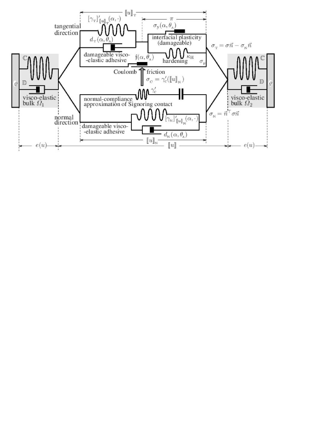
The conceptual rheological diagram corresponding to the part of the model,
namely
(2.3 2.4a 2 γ C ( [ [ u ] ] N ) ≫ γ N ( α , [ [ u ] ] N ) much-greater-than subscript 𝛾 C subscript delimited-[] delimited-[] 𝑢 N subscript 𝛾 N 𝛼 subscript delimited-[] delimited-[] 𝑢 N \gamma_{\scriptscriptstyle\textrm{C}}({\color[rgb]{0,0,0}\mathchoice{\big{[}\big{[}u\big{]}\big{]}_{{{}_{\rm N}}}}{[[u]]_{{{}_{\rm N}}}}{[\![u]\!]_{{{}_{\rm N}}}}{[\![u]\!]_{{{}_{\rm N}}}}})\gg\gamma_{{}_{\rm N}}(\alpha,{\color[rgb]{0,0,0}\mathchoice{\big{[}\big{[}u\big{]}\big{]}_{{{}_{\rm N}}}}{[[u]]_{{{}_{\rm N}}}}{[\![u]\!]_{{{}_{\rm N}}}}{[\![u]\!]_{{{}_{\rm N}}}}}) [ [ u ] ] N < 0 subscript delimited-[] delimited-[] 𝑢 N 0 {\color[rgb]{0,0,0}\mathchoice{\big{[}\big{[}u\big{]}\big{]}_{{{}_{\rm N}}}}{[[u]]_{{{}_{\rm N}}}}{[\![u]\!]_{{{}_{\rm N}}}}{[\![u]\!]_{{{}_{\rm N}}}}}<0 , otherwise rather σ N subscript 𝜎 N \sigma_{{{}_{\rm N}}} 2.3 4.6 .
The standard symbols are used for elastic and viscous elements
(springs and dashpots), respectively, and for the dry-friction-type
elements.
Figure 2: Schematic rheological model used on the adhesive interface
Γ C subscript Γ C \mathchoice{\varGamma_{\mbox{\tiny\rm C}}}{\varGamma_{\mbox{\tiny\rm C}}}{\varGamma_{\mbox{\tiny\rm C}}}{\varGamma_{\mbox{\tiny\rm C}}} π 𝜋 \pi the tangential
slip and the unilateral contact for the normal displacement.
Thermal expansion in the bulk
is not depicted, neither is evolution for delamination α 𝛼 \alpha s on Γ C subscript Γ C \mathchoice{\varGamma_{\mbox{\tiny\rm C}}}{\varGamma_{\mbox{\tiny\rm C}}}{\varGamma_{\mbox{\tiny\rm C}}}{\varGamma_{\mbox{\tiny\rm C}}}
3 A monolithic form and thermodynamics of the model
Let us briefly present the thermodynamics of the boundary-value
problem (2.3 2.5 This justifies the problem
physically. Moreover, adapting [38 , Sect. 5.3]
for our situation, a “monolithic”
(in the sense of simultaneous treatment of the ( d − 1 ) 𝑑 1 (d{-}1) d 𝑑 d 3.9
First, the underlying overall Helmholtz free energy
Ψ = Ψ ( e , [ [ u ] ] , π , α , θ A , θ B ) Ψ Ψ 𝑒 delimited-[] delimited-[] 𝑢 𝜋 𝛼 subscript 𝜃 A subscript 𝜃 B \varPsi=\varPsi(e,{\color[rgb]{0,0,0}\mathchoice{\big{[}\big{[}u\big{]}\big{]}}{[[u]]}{[\![u]\!]}{[\![u]\!]}},\pi,\alpha,\theta_{\scriptscriptstyle\textrm{A}},\theta_{\scriptscriptstyle\textrm{B}}) bulk (=volume) and an interface parts, i.e.
Ψ ( e , [ [ u ] ] , π , α , θ A , θ B ) = ∫ Γ C ψ A ( [ [ u ] ] , π , α , θ A , ∇ S π , ∇ S α ) d S + ∫ Ω ∖ Γ C ψ B ( e , θ B ) d x , Ψ 𝑒 delimited-[] delimited-[] 𝑢 𝜋 𝛼 subscript 𝜃 A subscript 𝜃 B subscript subscript Γ C subscript 𝜓 A delimited-[] delimited-[] 𝑢 𝜋 𝛼 subscript 𝜃 A subscript ∇ S 𝜋 subscript ∇ S 𝛼 differential-d 𝑆 subscript Ω subscript Γ C subscript 𝜓 B 𝑒 subscript 𝜃 B differential-d 𝑥 \displaystyle\varPsi(e,{\color[rgb]{0,0,0}\mathchoice{\big{[}\big{[}u\big{]}\big{]}}{[[u]]}{[\![u]\!]}{[\![u]\!]}},\pi,\alpha,\theta_{\scriptscriptstyle\textrm{A}},\theta_{\scriptscriptstyle\textrm{B}})=\int_{\mathchoice{\varGamma_{\mbox{\tiny\rm C}}}{\varGamma_{\mbox{\tiny\rm C}}}{\varGamma_{\mbox{\tiny\rm C}}}{\varGamma_{\mbox{\tiny\rm C}}}}\!\!\psi_{\scriptscriptstyle\textrm{\hskip 0.25002ptA}}({\color[rgb]{0,0,0}\mathchoice{\big{[}\big{[}u\big{]}\big{]}}{[[u]]}{[\![u]\!]}{[\![u]\!]}},\pi,\alpha,\theta_{\scriptscriptstyle\textrm{A}}{\color[rgb]{0,0,0},\nabla_{\scriptscriptstyle\textrm{S}}\pi,\nabla_{\scriptscriptstyle\textrm{S}}\alpha})\,\mathrm{d}S+\int_{\varOmega{\setminus}\mathchoice{\varGamma_{\mbox{\tiny\rm C}}}{\varGamma_{\mbox{\tiny\rm C}}}{\varGamma_{\mbox{\tiny\rm C}}}{\varGamma_{\mbox{\tiny\rm C}}}}\!\!\psi_{\scriptscriptstyle\textrm{\hskip 0.25002ptB}}(e,\theta_{\scriptscriptstyle\textrm{B}})\,\mathrm{d}x\,, (3.1a)
with ψ B subscript 𝜓 B \psi_{\scriptscriptstyle\textrm{\hskip 0.25002ptB}} ψ A subscript 𝜓 A \psi_{\scriptscriptstyle\textrm{\hskip 0.25002ptA}}
ψ B ( e , θ B ) subscript 𝜓 B 𝑒 subscript 𝜃 B \displaystyle\psi_{\scriptscriptstyle\textrm{\hskip 0.25002ptB}}(e,\theta_{\scriptscriptstyle\textrm{B}}) = 1 2 ℂ ( e − 𝔼 θ B + 𝔼 θ R ) : ( e − 𝔼 θ B + 𝔼 θ R ) − ( θ B − θ R ) 2 2 𝔹 : 𝔼 − ψ B 0 ( θ B ) : absent 1 2 ℂ 𝑒 𝔼 subscript 𝜃 B 𝔼 subscript 𝜃 R 𝑒 𝔼 subscript 𝜃 B 𝔼 subscript 𝜃 R superscript subscript 𝜃 B subscript 𝜃 R 2 2 𝔹 : 𝔼 subscript subscript 𝜓 B 0 subscript 𝜃 B \displaystyle=\frac{1}{2}\mathbb{C}(e{-}\mathbb{E}\theta_{\scriptscriptstyle\textrm{B}}{\color[rgb]{0,0,0}{{+}\mathbb{E}\theta_{{}_{\rm R}}}}){:}(e{-}\mathbb{E}\theta_{\scriptscriptstyle\textrm{B}}{\color[rgb]{0,0,0}{{+}\mathbb{E}\theta_{{}_{\rm R}}}})-\frac{(\theta_{\scriptscriptstyle\textrm{B}}{\color[rgb]{0,0,0}{{-}\theta_{{}_{\rm R}})}}^{2}}{2}\mathbb{B}{:}\mathbb{E}-{\psi_{\scriptscriptstyle\textrm{\hskip 0.25002ptB}}}_{0}(\theta_{\scriptscriptstyle\textrm{B}})
= 1 2 ℂ e : e − ( θ B − θ R ) 𝔹 : e − ψ B 0 ( θ B ) with 𝔹 := ℂ 𝔼 . : absent 1 2 ℂ 𝑒 𝑒 subscript 𝜃 B subscript 𝜃 R 𝔹 : assign 𝑒 subscript subscript 𝜓 B 0 subscript 𝜃 B with 𝔹
ℂ 𝔼 \displaystyle=\frac{1}{2}\mathbb{C}e{:}e-(\theta_{\scriptscriptstyle\textrm{B}}{-}\theta_{{}_{\rm R}})\mathbb{B}{:}e-{\psi_{\scriptscriptstyle\textrm{\hskip 0.25002ptB}}}_{0}(\theta_{\scriptscriptstyle\textrm{B}})\quad\text{ with }\ \mathbb{B}:=\mathbb{C}\mathbb{E}. (3.1b)
Here 1 2 ℂ e : e : 1 2 ℂ 𝑒 𝑒 \frac{1}{2}\mathbb{C}e{:}e mechanical part of the
internal energy in the bulk , while − ψ B 0 ( θ B ) subscript subscript 𝜓 B 0 subscript 𝜃 B -{\psi_{\scriptscriptstyle\textrm{\hskip 0.25002ptB}}}_{0}(\theta_{\scriptscriptstyle\textrm{B}}) thermal part of the free energy . Hereafter, we shall assume that
ψ B 0 : ( 0 , + ∞ ) → ℝ : subscript subscript 𝜓 B 0 → 0 ℝ {\psi_{\scriptscriptstyle\textrm{\hskip 0.25002ptB}}}_{0}:(0,+\infty)\to{\mathbb{R}} (3.1c)
The specific contact interface energy
ψ A ( [ [ u ] ] , π , α , θ A , ∇ S π , ∇ S α ) subscript 𝜓 A delimited-[] delimited-[] 𝑢 𝜋 𝛼 subscript 𝜃 A subscript ∇ S 𝜋 subscript ∇ S 𝛼 \psi_{\scriptscriptstyle\textrm{\hskip 0.25002ptA}}({\color[rgb]{0,0,0}\mathchoice{\big{[}\big{[}u\big{]}\big{]}}{[[u]]}{[\![u]\!]}{[\![u]\!]}},\pi,\alpha,\theta_{\scriptscriptstyle\textrm{A}}{\color[rgb]{0,0,0},\nabla_{\scriptscriptstyle\textrm{S}}\pi,\nabla_{\scriptscriptstyle\textrm{S}}\alpha})
ψ A ( [ [ u ] ] , π , α , θ A , ∇ S π , ∇ S α ) = { γ T ( α , [ [ u ] ] T − π ) + γ N ( α , [ [ u ] ] N ) + γ C ( [ [ u ] ] N ) + κ H 2 | π | 2 + κ 1 2 | ∇ S π | 2 + κ 2 2 | ∇ S α | 2 − a 0 ( α ) − b 0 ( α ) θ A − ψ A 0 ( θ A ) if 0 ≤ α ≤ 1 a.e. on Γ C , + ∞ otherwise . subscript 𝜓 A delimited-[] delimited-[] 𝑢 𝜋 𝛼 subscript 𝜃 A subscript ∇ S 𝜋 subscript ∇ S 𝛼 cases subscript 𝛾 T 𝛼 subscript delimited-[] delimited-[] 𝑢 T 𝜋 subscript 𝛾 N 𝛼 subscript delimited-[] delimited-[] 𝑢 N subscript 𝛾 C subscript delimited-[] delimited-[] 𝑢 N otherwise subscript 𝜅 H 2 superscript 𝜋 2 subscript 𝜅 1 2 superscript subscript ∇ S 𝜋 2 subscript 𝜅 2 2 superscript subscript ∇ S 𝛼 2 otherwise subscript 𝑎 0 𝛼 subscript 𝑏 0 𝛼 subscript 𝜃 A subscript subscript 𝜓 A 0 subscript 𝜃 A if 0 ≤ α ≤ 1 a.e. on Γ C otherwise \psi_{\scriptscriptstyle\textrm{\hskip 0.25002ptA}}\big{(}{\color[rgb]{0,0,0}\mathchoice{\big{[}\big{[}u\big{]}\big{]}}{[[u]]}{[\![u]\!]}{[\![u]\!]}},\pi,\alpha,\theta_{\scriptscriptstyle\textrm{A}}{\color[rgb]{0,0,0},\nabla_{\scriptscriptstyle\textrm{S}}\pi,\nabla_{\scriptscriptstyle\textrm{S}}\alpha}\big{)}=\begin{cases}\displaystyle{\gamma_{{{}_{\rm T}}}\big{(}\alpha,{\color[rgb]{0,0,0}\mathchoice{\big{[}\big{[}u\big{]}\big{]}_{{{}_{\rm T}}}}{[[u]]_{{{}_{\rm T}}}}{[\![u]\!]_{{{}_{\rm T}}}}{[\![u]\!]_{{{}_{\rm T}}}}}\!{-}\pi\big{)}+\gamma_{{{}_{\rm N}}}\big{(}\alpha,{\color[rgb]{0,0,0}\mathchoice{\big{[}\big{[}u\big{]}\big{]}_{{{}_{\rm N}}}}{[[u]]_{{{}_{\rm N}}}}{[\![u]\!]_{{{}_{\rm N}}}}{[\![u]\!]_{{{}_{\rm N}}}}}\big{)}+\gamma_{\scriptscriptstyle\textrm{C}}\big{(}{\color[rgb]{0,0,0}\mathchoice{\big{[}\big{[}u\big{]}\big{]}_{{{}_{\rm N}}}}{[[u]]_{{{}_{\rm N}}}}{[\![u]\!]_{{{}_{\rm N}}}}{[\![u]\!]_{{{}_{\rm N}}}}}\big{)}}\\[3.00003pt]
\displaystyle{\ \ \ \ \ +\frac{\kappa_{\rm H}}{2}|\pi|^{2}+\frac{\kappa_{1}}{2}|\nabla_{\scriptscriptstyle\textrm{S}}\pi|^{2}+\frac{\kappa_{2}}{2}|\nabla_{\scriptscriptstyle\textrm{S}}\alpha|^{2}}\\[3.00003pt]
\displaystyle{\ \ \ \ \ -\,a_{0}(\alpha)-b_{0}(\alpha)\theta_{\scriptscriptstyle\textrm{A}}-{\psi_{\scriptscriptstyle\textrm{\hskip 0.25002ptA}}}_{\,0}(\theta_{\scriptscriptstyle\textrm{A}})}&\mbox{if $\ 0\!\leq\!\alpha\!\leq\!1$ a.e.~{}on $\mathchoice{\varGamma_{\mbox{\tiny\rm C}}}{\varGamma_{\mbox{\tiny\rm C}}}{\varGamma_{\mbox{\tiny\rm C}}}{\varGamma_{\mbox{\tiny\rm C}}}$},\\
+\infty&\text{otherwise}.\end{cases} (3.1d)
The terms a 0 ( α ) + b 0 ( α ) θ A subscript 𝑎 0 𝛼 subscript 𝑏 0 𝛼 subscript 𝜃 A a_{0}(\alpha)+b_{0}(\alpha)\theta_{\scriptscriptstyle\textrm{A}}
The typical
choice
for γ N subscript 𝛾 N \gamma_{{{}_{\rm N}}} γ T subscript 𝛾 T \gamma_{{{}_{\rm T}}} variable α 𝛼 \alpha elastic adhesive
γ N ( α , [ [ u ] ] N ) = 1 2 κ N ( α ) | [ [ u ] ] N | 2 and γ T ( α , [ [ u ] ] T ) = 1 2 κ T ( α ) | [ [ u ] ] T | 2 , formulae-sequence subscript 𝛾 N 𝛼 subscript delimited-[] delimited-[] 𝑢 N 1 2 subscript 𝜅 N 𝛼 superscript subscript delimited-[] delimited-[] 𝑢 N 2 and
subscript 𝛾 T 𝛼 subscript delimited-[] delimited-[] 𝑢 T 1 2 subscript 𝜅 T 𝛼 superscript subscript delimited-[] delimited-[] 𝑢 T 2 \gamma_{{{}_{\rm N}}}\big{(}\alpha,\mbox{${\color[rgb]{0,0,0}\mathchoice{\big{[}\big{[}u\big{]}\big{]}_{{{}_{\rm N}}}}{[[u]]_{{{}_{\rm N}}}}{[\![u]\!]_{{{}_{\rm N}}}}{[\![u]\!]_{{{}_{\rm N}}}}}$}\big{)}=\frac{1}{2}\kappa_{{{}_{\rm N}}}(\alpha)\big{|}\mbox{${\color[rgb]{0,0,0}\mathchoice{\big{[}\big{[}u\big{]}\big{]}_{{{}_{\rm N}}}}{[[u]]_{{{}_{\rm N}}}}{[\![u]\!]_{{{}_{\rm N}}}}{[\![u]\!]_{{{}_{\rm N}}}}}$}\big{|}^{2}\quad\text{and}\quad\gamma_{{{}_{\rm T}}}\big{(}\alpha,\mbox{${\color[rgb]{0,0,0}\mathchoice{\big{[}\big{[}u\big{]}\big{]}_{{{}_{\rm T}}}}{[[u]]_{{{}_{\rm T}}}}{[\![u]\!]_{{{}_{\rm T}}}}{[\![u]\!]_{{{}_{\rm T}}}}}$}\big{)}=\frac{1}{2}\kappa_{{{}_{\rm T}}}(\alpha)\big{|}\mbox{${\color[rgb]{0,0,0}\mathchoice{\big{[}\big{[}u\big{]}\big{]}_{{{}_{\rm T}}}}{[[u]]_{{{}_{\rm T}}}}{[\![u]\!]_{{{}_{\rm T}}}}{[\![u]\!]_{{{}_{\rm T}}}}}$}\big{|}^{2}, (3.2)
while the typical
choice for γ C subscript 𝛾 C \gamma_{\scriptscriptstyle\textrm{C}}
γ C ( [ [ u ] ] N ) = { 0 if [ [ u ] ] N ≥ 0 , 1 p κ C ( − [ [ u ] ] N ) p if [ [ u ] ] N < 0 , subscript 𝛾 C subscript delimited-[] delimited-[] 𝑢 N cases 0 if subscript delimited-[] delimited-[] 𝑢 N 0 1 𝑝 subscript 𝜅 C superscript subscript delimited-[] delimited-[] 𝑢 N 𝑝 if subscript delimited-[] delimited-[] 𝑢 N 0 \displaystyle\gamma_{\scriptscriptstyle\textrm{C}}\big{(}{\color[rgb]{0,0,0}\mathchoice{\big{[}\big{[}u\big{]}\big{]}_{{{}_{\rm N}}}}{[[u]]_{{{}_{\rm N}}}}{[\![u]\!]_{{{}_{\rm N}}}}{[\![u]\!]_{{{}_{\rm N}}}}}\big{)}=\begin{cases}0&\text{if }{\color[rgb]{0,0,0}\mathchoice{\big{[}\big{[}u\big{]}\big{]}_{{{}_{\rm N}}}}{[[u]]_{{{}_{\rm N}}}}{[\![u]\!]_{{{}_{\rm N}}}}{[\![u]\!]_{{{}_{\rm N}}}}}\geq 0,\\
\frac{1}{p}\kappa_{{}_{\rm C}}\big{(}-{\color[rgb]{0,0,0}\mathchoice{\big{[}\big{[}u\big{]}\big{]}_{{{}_{\rm N}}}}{[[u]]_{{{}_{\rm N}}}}{[\![u]\!]_{{{}_{\rm N}}}}{[\![u]\!]_{{{}_{\rm N}}}}}\big{)}^{p}&\text{if }{\color[rgb]{0,0,0}\mathchoice{\big{[}\big{[}u\big{]}\big{]}_{{{}_{\rm N}}}}{[[u]]_{{{}_{\rm N}}}}{[\![u]\!]_{{{}_{\rm N}}}}{[\![u]\!]_{{{}_{\rm N}}}}}<0,\end{cases} (unilateral normal-compliance) (3.3) which is to approximate for κ C → + ∞ → subscript 𝜅 C \kappa_{{}_{\rm C}}\to+\infty γ C ( [ [ u ] ] N ) = + ∞ subscript 𝛾 C subscript delimited-[] delimited-[] 𝑢 N \gamma_{\scriptscriptstyle\textrm{C}}({\color[rgb]{0,0,0}\mathchoice{\big{[}\big{[}u\big{]}\big{]}_{{{}_{\rm N}}}}{[[u]]_{{{}_{\rm N}}}}{[\![u]\!]_{{{}_{\rm N}}}}{[\![u]\!]_{{{}_{\rm N}}}}})=+\infty [ [ u ] ] N < 0 subscript delimited-[] delimited-[] 𝑢 N 0 {\color[rgb]{0,0,0}\mathchoice{\big{[}\big{[}u\big{]}\big{]}_{{{}_{\rm N}}}}{[[u]]_{{{}_{\rm N}}}}{[\![u]\!]_{{{}_{\rm N}}}}{[\![u]\!]_{{{}_{\rm N}}}}}<0 γ C ( [ [ u ] ] N ) = 0 subscript 𝛾 C subscript delimited-[] delimited-[] 𝑢 N 0 \gamma_{\scriptscriptstyle\textrm{C}}({\color[rgb]{0,0,0}\mathchoice{\big{[}\big{[}u\big{]}\big{]}_{{{}_{\rm N}}}}{[[u]]_{{{}_{\rm N}}}}{[\![u]\!]_{{{}_{\rm N}}}}{[\![u]\!]_{{{}_{\rm N}}}}})=0 Γ C subscript Γ C \mathchoice{\varGamma_{\mbox{\tiny\rm C}}}{\varGamma_{\mbox{\tiny\rm C}}}{\varGamma_{\mbox{\tiny\rm C}}}{\varGamma_{\mbox{\tiny\rm C}}} 3.3 p 𝑝 p d = 2 𝑑 2 d=2 p ≤ 4 𝑝 4 p\leq 4 d = 3 𝑑 3 d=3 u ∈ H 1 ( Ω ∖ Γ C ; ℝ d ) 𝑢 superscript 𝐻 1 Ω subscript Γ C superscript ℝ 𝑑
u\in H^{1}(\varOmega{\setminus}\mathchoice{\varGamma_{\mbox{\tiny\rm C}}}{\varGamma_{\mbox{\tiny\rm C}}}{\varGamma_{\mbox{\tiny\rm C}}}{\varGamma_{\mbox{\tiny\rm C}}};{\mathbb{R}}^{d}) [ [ u ] ] N ∈ H 1 / 2 ( Γ C ) ⊂ L 4 ( Γ C ) subscript delimited-[] delimited-[] 𝑢 N superscript 𝐻 1 2 subscript Γ C superscript 𝐿 4 subscript Γ C \mathchoice{\big{[}\big{[}u\big{]}\big{]}_{{{}_{\rm N}}}}{[[u]]_{{{}_{\rm N}}}}{[\![u]\!]_{{{}_{\rm N}}}}{[\![u]\!]_{{{}_{\rm N}}}}\in H^{1/2}(\mathchoice{\varGamma_{\mbox{\tiny\rm C}}}{\varGamma_{\mbox{\tiny\rm C}}}{\varGamma_{\mbox{\tiny\rm C}}}{\varGamma_{\mbox{\tiny\rm C}}})\subset L^{4}(\mathchoice{\varGamma_{\mbox{\tiny\rm C}}}{\varGamma_{\mbox{\tiny\rm C}}}{\varGamma_{\mbox{\tiny\rm C}}}{\varGamma_{\mbox{\tiny\rm C}}}) d = 3 𝑑 3 d=3
γ C ( [ [ u ] ] N ) = { 0 if [ [ u ] ] N = 0 , ∞ if [ [ u ] ] N ≠ 0 . subscript 𝛾 C subscript delimited-[] delimited-[] 𝑢 N cases 0 if subscript delimited-[] delimited-[] 𝑢 N 0 if subscript delimited-[] delimited-[] 𝑢 N 0 \displaystyle\gamma_{\scriptscriptstyle\textrm{C}}\big{(}{\color[rgb]{0,0,0}\mathchoice{\big{[}\big{[}u\big{]}\big{]}_{{{}_{\rm N}}}}{[[u]]_{{{}_{\rm N}}}}{[\![u]\!]_{{{}_{\rm N}}}}{[\![u]\!]_{{{}_{\rm N}}}}}\big{)}=\begin{cases}0&\text{if }{\color[rgb]{0,0,0}\mathchoice{\big{[}\big{[}u\big{]}\big{]}_{{{}_{\rm N}}}}{[[u]]_{{{}_{\rm N}}}}{[\![u]\!]_{{{}_{\rm N}}}}{[\![u]\!]_{{{}_{\rm N}}}}}=0,\\
\infty&\text{if }{\color[rgb]{0,0,0}\mathchoice{\big{[}\big{[}u\big{]}\big{]}_{{{}_{\rm N}}}}{[[u]]_{{{}_{\rm N}}}}{[\![u]\!]_{{{}_{\rm N}}}}{[\![u]\!]_{{{}_{\rm N}}}}}\neq 0.\end{cases} (bilateral contact) (3.4)
Yet, it should be mention that the normal compliance is more
natural is our a setting than the Signorini condition which is a bit
artificial because, when the adhesive is rigid, the issue is of fracture
and not debonding.
The other underlying ingredient of the model is
the overall
pseudo-potential of the dissipative forces Ξ Ξ \varXi contact-interface contributions ξ A subscript 𝜉 A \xi_{\scriptscriptstyle\textrm{\hskip 0.25002ptA}} ξ B subscript 𝜉 B \xi_{\scriptscriptstyle\textrm{\hskip 0.25002ptB}}
Ξ ( [ [ u ] ] , α , θ A , θ B ; e . , [ [ u . ] ] , π . , α . ) := ∫ Γ C ξ A ( [ [ u ] ] , α , θ A , [ [ u . ] ] , π . , α . ) d S + ∫ Ω ∖ Γ C ξ B ( θ B ; e . ) d x ; assign Ξ delimited-[] delimited-[] 𝑢 𝛼 subscript 𝜃 A subscript 𝜃 B superscript 𝑒 . delimited-[] delimited-[] superscript 𝑢 . superscript 𝜋 . superscript 𝛼 . subscript subscript Γ C subscript 𝜉 A delimited-[] delimited-[] 𝑢 𝛼 subscript 𝜃 A delimited-[] delimited-[] superscript 𝑢 . superscript 𝜋 . superscript 𝛼 . differential-d 𝑆 subscript Ω subscript Γ C subscript 𝜉 B subscript 𝜃 B superscript 𝑒 .
differential-d 𝑥 \displaystyle\varXi\big{(}\mathchoice{\big{[}\big{[}u\big{]}\big{]}}{[[u]]}{[\![u]\!]}{[\![u]\!]},\alpha,\theta_{\scriptscriptstyle\textrm{A}},\theta_{\scriptscriptstyle\textrm{B}};\mathchoice{{\buildrel\hskip 1.00006pt\text{\LARGE.}\over{e}}}{{\buildrel\hskip 1.00006pt\text{\Large.}\over{e}}}{{\buildrel\hskip 1.00006pt\text{\large.}\over{e}}}{{\buildrel\hskip 1.00006pt\text{\large.}\over{e}}},{\color[rgb]{0,0,0}{\mathchoice{\big{[}\big{[}\mathchoice{{\buildrel\hskip 1.00006pt\text{\LARGE.}\over{u}}}{{\buildrel\hskip 1.00006pt\text{\Large.}\over{u}}}{{\buildrel\hskip 1.00006pt\text{\large.}\over{u}}}{{\buildrel\hskip 1.00006pt\text{\large.}\over{u}}}\big{]}\big{]}}{[[\mathchoice{{\buildrel\hskip 1.00006pt\text{\LARGE.}\over{u}}}{{\buildrel\hskip 1.00006pt\text{\Large.}\over{u}}}{{\buildrel\hskip 1.00006pt\text{\large.}\over{u}}}{{\buildrel\hskip 1.00006pt\text{\large.}\over{u}}}]]}{[\![\mathchoice{{\buildrel\hskip 1.00006pt\text{\LARGE.}\over{u}}}{{\buildrel\hskip 1.00006pt\text{\Large.}\over{u}}}{{\buildrel\hskip 1.00006pt\text{\large.}\over{u}}}{{\buildrel\hskip 1.00006pt\text{\large.}\over{u}}}]\!]}{[\![\mathchoice{{\buildrel\hskip 1.00006pt\text{\LARGE.}\over{u}}}{{\buildrel\hskip 1.00006pt\text{\Large.}\over{u}}}{{\buildrel\hskip 1.00006pt\text{\large.}\over{u}}}{{\buildrel\hskip 1.00006pt\text{\large.}\over{u}}}]\!]}}},\mathchoice{{\buildrel\hskip 1.00006pt\text{\LARGE.}\over{\pi}}}{{\buildrel\hskip 1.00006pt\text{\Large.}\over{\pi}}}{{\buildrel\hskip 1.00006pt\text{\large.}\over{\pi}}}{{\buildrel\hskip 1.00006pt\text{\large.}\over{\pi}}},\mathchoice{{\buildrel\hskip 1.00006pt\text{\LARGE.}\over{\alpha}}}{{\buildrel\hskip 1.00006pt\text{\Large.}\over{\alpha}}}{{\buildrel\hskip 1.00006pt\text{\large.}\over{\alpha}}}{{\buildrel\hskip 1.00006pt\text{\large.}\over{\alpha}}}\big{)}:=\int_{\mathchoice{\varGamma_{\mbox{\tiny\rm C}}}{\varGamma_{\mbox{\tiny\rm C}}}{\varGamma_{\mbox{\tiny\rm C}}}{\varGamma_{\mbox{\tiny\rm C}}}}\!\xi_{\scriptscriptstyle\textrm{\hskip 0.25002ptA}}\big{(}\mathchoice{\big{[}\big{[}u\big{]}\big{]}}{[[u]]}{[\![u]\!]}{[\![u]\!]},\alpha,\theta_{\scriptscriptstyle\textrm{A}},{\color[rgb]{0,0,0}{\mathchoice{\big{[}\big{[}\mathchoice{{\buildrel\hskip 1.00006pt\text{\LARGE.}\over{u}}}{{\buildrel\hskip 1.00006pt\text{\Large.}\over{u}}}{{\buildrel\hskip 1.00006pt\text{\large.}\over{u}}}{{\buildrel\hskip 1.00006pt\text{\large.}\over{u}}}\big{]}\big{]}}{[[\mathchoice{{\buildrel\hskip 1.00006pt\text{\LARGE.}\over{u}}}{{\buildrel\hskip 1.00006pt\text{\Large.}\over{u}}}{{\buildrel\hskip 1.00006pt\text{\large.}\over{u}}}{{\buildrel\hskip 1.00006pt\text{\large.}\over{u}}}]]}{[\![\mathchoice{{\buildrel\hskip 1.00006pt\text{\LARGE.}\over{u}}}{{\buildrel\hskip 1.00006pt\text{\Large.}\over{u}}}{{\buildrel\hskip 1.00006pt\text{\large.}\over{u}}}{{\buildrel\hskip 1.00006pt\text{\large.}\over{u}}}]\!]}{[\![\mathchoice{{\buildrel\hskip 1.00006pt\text{\LARGE.}\over{u}}}{{\buildrel\hskip 1.00006pt\text{\Large.}\over{u}}}{{\buildrel\hskip 1.00006pt\text{\large.}\over{u}}}{{\buildrel\hskip 1.00006pt\text{\large.}\over{u}}}]\!]}}},\mathchoice{{\buildrel\hskip 1.00006pt\text{\LARGE.}\over{\pi}}}{{\buildrel\hskip 1.00006pt\text{\Large.}\over{\pi}}}{{\buildrel\hskip 1.00006pt\text{\large.}\over{\pi}}}{{\buildrel\hskip 1.00006pt\text{\large.}\over{\pi}}},\mathchoice{{\buildrel\hskip 1.00006pt\text{\LARGE.}\over{\alpha}}}{{\buildrel\hskip 1.00006pt\text{\Large.}\over{\alpha}}}{{\buildrel\hskip 1.00006pt\text{\large.}\over{\alpha}}}{{\buildrel\hskip 1.00006pt\text{\large.}\over{\alpha}}}\big{)}\,\mathrm{d}S+\int_{\varOmega{\setminus}\mathchoice{\varGamma_{\mbox{\tiny\rm C}}}{\varGamma_{\mbox{\tiny\rm C}}}{\varGamma_{\mbox{\tiny\rm C}}}{\varGamma_{\mbox{\tiny\rm C}}}}\!\!\xi_{\scriptscriptstyle\textrm{\hskip 0.25002ptB}}(\theta_{\scriptscriptstyle\textrm{B}};\mathchoice{{\buildrel\hskip 1.00006pt\text{\LARGE.}\over{e}}}{{\buildrel\hskip 1.00006pt\text{\Large.}\over{e}}}{{\buildrel\hskip 1.00006pt\text{\large.}\over{e}}}{{\buildrel\hskip 1.00006pt\text{\large.}\over{e}}})\,\mathrm{d}x; (3.5)
where
ξ A ( [ [ u ] ] N , α , θ A ; [ [ u . ] ] , α . , π . ) : = 𝔣 ( α , θ A ) γ C ′ ( [ [ u ] ] N ) | [ [ u . ] ] T | + σ y ( α , θ A ) | π . | \displaystyle\xi_{\scriptscriptstyle\textrm{\hskip 0.25002ptA}}\big{(}{\color[rgb]{0,0,0}\mathchoice{\big{[}\big{[}u\big{]}\big{]}_{{{}_{\rm N}}}}{[[u]]_{{{}_{\rm N}}}}{[\![u]\!]_{{{}_{\rm N}}}}{[\![u]\!]_{{{}_{\rm N}}}}},\alpha,\theta_{\scriptscriptstyle\textrm{A}};{\color[rgb]{0,0,0}\mathchoice{\big{[}\big{[}\mathchoice{{\buildrel\hskip 1.00006pt\text{\LARGE.}\over{u}}}{{\buildrel\hskip 1.00006pt\text{\Large.}\over{u}}}{{\buildrel\hskip 1.00006pt\text{\large.}\over{u}}}{{\buildrel\hskip 1.00006pt\text{\large.}\over{u}}}\big{]}\big{]}}{[[\mathchoice{{\buildrel\hskip 1.00006pt\text{\LARGE.}\over{u}}}{{\buildrel\hskip 1.00006pt\text{\Large.}\over{u}}}{{\buildrel\hskip 1.00006pt\text{\large.}\over{u}}}{{\buildrel\hskip 1.00006pt\text{\large.}\over{u}}}]]}{[\![\mathchoice{{\buildrel\hskip 1.00006pt\text{\LARGE.}\over{u}}}{{\buildrel\hskip 1.00006pt\text{\Large.}\over{u}}}{{\buildrel\hskip 1.00006pt\text{\large.}\over{u}}}{{\buildrel\hskip 1.00006pt\text{\large.}\over{u}}}]\!]}{[\![\mathchoice{{\buildrel\hskip 1.00006pt\text{\LARGE.}\over{u}}}{{\buildrel\hskip 1.00006pt\text{\Large.}\over{u}}}{{\buildrel\hskip 1.00006pt\text{\large.}\over{u}}}{{\buildrel\hskip 1.00006pt\text{\large.}\over{u}}}]\!]}},\mathchoice{{\buildrel\hskip 1.00006pt\text{\LARGE.}\over{\alpha}}}{{\buildrel\hskip 1.00006pt\text{\Large.}\over{\alpha}}}{{\buildrel\hskip 1.00006pt\text{\large.}\over{\alpha}}}{{\buildrel\hskip 1.00006pt\text{\large.}\over{\alpha}}},\mathchoice{{\buildrel\hskip 1.00006pt\text{\LARGE.}\over{\pi}}}{{\buildrel\hskip 1.00006pt\text{\Large.}\over{\pi}}}{{\buildrel\hskip 1.00006pt\text{\large.}\over{\pi}}}{{\buildrel\hskip 1.00006pt\text{\large.}\over{\pi}}}\big{)}:=\mathfrak{f}(\alpha,\theta_{\scriptscriptstyle\textrm{A}})\gamma_{\scriptscriptstyle\textrm{C}}^{\prime}({\color[rgb]{0,0,0}\mathchoice{\big{[}\big{[}u\big{]}\big{]}_{{{}_{\rm N}}}}{[[u]]_{{{}_{\rm N}}}}{[\![u]\!]_{{{}_{\rm N}}}}{[\![u]\!]_{{{}_{\rm N}}}}})\big{|}{\color[rgb]{0,0,0}\mathchoice{\big{[}\big{[}\mathchoice{{\buildrel\hskip 1.00006pt\text{\LARGE.}\over{u}}}{{\buildrel\hskip 1.00006pt\text{\Large.}\over{u}}}{{\buildrel\hskip 1.00006pt\text{\large.}\over{u}}}{{\buildrel\hskip 1.00006pt\text{\large.}\over{u}}}\big{]}\big{]}_{{{}_{\rm T}}}}{[[\mathchoice{{\buildrel\hskip 1.00006pt\text{\LARGE.}\over{u}}}{{\buildrel\hskip 1.00006pt\text{\Large.}\over{u}}}{{\buildrel\hskip 1.00006pt\text{\large.}\over{u}}}{{\buildrel\hskip 1.00006pt\text{\large.}\over{u}}}]]_{{{}_{\rm T}}}}{[\![\mathchoice{{\buildrel\hskip 1.00006pt\text{\LARGE.}\over{u}}}{{\buildrel\hskip 1.00006pt\text{\Large.}\over{u}}}{{\buildrel\hskip 1.00006pt\text{\large.}\over{u}}}{{\buildrel\hskip 1.00006pt\text{\large.}\over{u}}}]\!]_{{{}_{\rm T}}}}{[\![\mathchoice{{\buildrel\hskip 1.00006pt\text{\LARGE.}\over{u}}}{{\buildrel\hskip 1.00006pt\text{\Large.}\over{u}}}{{\buildrel\hskip 1.00006pt\text{\large.}\over{u}}}{{\buildrel\hskip 1.00006pt\text{\large.}\over{u}}}]\!]_{{{}_{\rm T}}}}}\big{|}+\sigma_{\rm y}(\alpha,\theta_{\scriptscriptstyle\textrm{A}})\big{|}\mathchoice{{\buildrel\hskip 1.00006pt\text{\LARGE.}\over{\pi}}}{{\buildrel\hskip 1.00006pt\text{\Large.}\over{\pi}}}{{\buildrel\hskip 1.00006pt\text{\large.}\over{\pi}}}{{\buildrel\hskip 1.00006pt\text{\large.}\over{\pi}}}\big{|}
+ α . ∂ α . a 1 ( [ [ u . ] ] , α , θ A , α . ) + d T ( α , θ A ) 2 | [ [ u . ] ] T − π . | 2 + d N ( α , θ A ) 2 [ [ u . ] ] N 2 , \displaystyle\hskip 110.00017pt+{\color[rgb]{0,0,0}\mathchoice{{\buildrel\hskip 1.00006pt\text{\LARGE.}\over{\alpha}}}{{\buildrel\hskip 1.00006pt\text{\Large.}\over{\alpha}}}{{\buildrel\hskip 1.00006pt\text{\large.}\over{\alpha}}}{{\buildrel\hskip 1.00006pt\text{\large.}\over{\alpha}}}\partial_{\mathchoice{{\buildrel\hskip 0.70004pt\text{\LARGE.}\over{\alpha}}}{{\buildrel\hskip 0.70004pt\text{\Large.}\over{\alpha}}}{{\buildrel\hskip 0.70004pt\text{\large.}\over{\alpha}}}{{\buildrel\hskip 0.70004pt\text{\large.}\over{\alpha}}}}}a_{1}\big{(}{\color[rgb]{0,0,0}\mathchoice{\big{[}\big{[}\mathchoice{{\buildrel\hskip 1.00006pt\text{\LARGE.}\over{u}}}{{\buildrel\hskip 1.00006pt\text{\Large.}\over{u}}}{{\buildrel\hskip 1.00006pt\text{\large.}\over{u}}}{{\buildrel\hskip 1.00006pt\text{\large.}\over{u}}}\big{]}\big{]}}{[[\mathchoice{{\buildrel\hskip 1.00006pt\text{\LARGE.}\over{u}}}{{\buildrel\hskip 1.00006pt\text{\Large.}\over{u}}}{{\buildrel\hskip 1.00006pt\text{\large.}\over{u}}}{{\buildrel\hskip 1.00006pt\text{\large.}\over{u}}}]]}{[\![\mathchoice{{\buildrel\hskip 1.00006pt\text{\LARGE.}\over{u}}}{{\buildrel\hskip 1.00006pt\text{\Large.}\over{u}}}{{\buildrel\hskip 1.00006pt\text{\large.}\over{u}}}{{\buildrel\hskip 1.00006pt\text{\large.}\over{u}}}]\!]}{[\![\mathchoice{{\buildrel\hskip 1.00006pt\text{\LARGE.}\over{u}}}{{\buildrel\hskip 1.00006pt\text{\Large.}\over{u}}}{{\buildrel\hskip 1.00006pt\text{\large.}\over{u}}}{{\buildrel\hskip 1.00006pt\text{\large.}\over{u}}}]\!]}},{\color[rgb]{0,0,0}{\alpha,}}\theta_{\scriptscriptstyle\textrm{A}},\mathchoice{{\buildrel\hskip 1.00006pt\text{\LARGE.}\over{\alpha}}}{{\buildrel\hskip 1.00006pt\text{\Large.}\over{\alpha}}}{{\buildrel\hskip 1.00006pt\text{\large.}\over{\alpha}}}{{\buildrel\hskip 1.00006pt\text{\large.}\over{\alpha}}}\big{)}+\frac{d_{{}_{\rm T}}(\alpha,\theta_{\scriptscriptstyle\textrm{A}})}{{\color[rgb]{0,0,0}2}}\big{|}{\color[rgb]{0,0,0}\mathchoice{\big{[}\big{[}\mathchoice{{\buildrel\hskip 1.00006pt\text{\LARGE.}\over{u}}}{{\buildrel\hskip 1.00006pt\text{\Large.}\over{u}}}{{\buildrel\hskip 1.00006pt\text{\large.}\over{u}}}{{\buildrel\hskip 1.00006pt\text{\large.}\over{u}}}\big{]}\big{]}_{{{}_{\rm T}}}}{[[\mathchoice{{\buildrel\hskip 1.00006pt\text{\LARGE.}\over{u}}}{{\buildrel\hskip 1.00006pt\text{\Large.}\over{u}}}{{\buildrel\hskip 1.00006pt\text{\large.}\over{u}}}{{\buildrel\hskip 1.00006pt\text{\large.}\over{u}}}]]_{{{}_{\rm T}}}}{[\![\mathchoice{{\buildrel\hskip 1.00006pt\text{\LARGE.}\over{u}}}{{\buildrel\hskip 1.00006pt\text{\Large.}\over{u}}}{{\buildrel\hskip 1.00006pt\text{\large.}\over{u}}}{{\buildrel\hskip 1.00006pt\text{\large.}\over{u}}}]\!]_{{{}_{\rm T}}}}{[\![\mathchoice{{\buildrel\hskip 1.00006pt\text{\LARGE.}\over{u}}}{{\buildrel\hskip 1.00006pt\text{\Large.}\over{u}}}{{\buildrel\hskip 1.00006pt\text{\large.}\over{u}}}{{\buildrel\hskip 1.00006pt\text{\large.}\over{u}}}]\!]_{{{}_{\rm T}}}}}{-}\mathchoice{{\buildrel\hskip 1.00006pt\text{\LARGE.}\over{\pi}}}{{\buildrel\hskip 1.00006pt\text{\Large.}\over{\pi}}}{{\buildrel\hskip 1.00006pt\text{\large.}\over{\pi}}}{{\buildrel\hskip 1.00006pt\text{\large.}\over{\pi}}}\big{|}^{2}+\frac{d_{{}_{\rm N}}(\alpha,\theta_{\scriptscriptstyle\textrm{A}})}{{\color[rgb]{0,0,0}2}}{\color[rgb]{0,0,0}\mathchoice{\big{[}\big{[}\mathchoice{{\buildrel\hskip 1.00006pt\text{\LARGE.}\over{u}}}{{\buildrel\hskip 1.00006pt\text{\Large.}\over{u}}}{{\buildrel\hskip 1.00006pt\text{\large.}\over{u}}}{{\buildrel\hskip 1.00006pt\text{\large.}\over{u}}}\big{]}\big{]}_{{{}_{\rm N}}}}{[[\mathchoice{{\buildrel\hskip 1.00006pt\text{\LARGE.}\over{u}}}{{\buildrel\hskip 1.00006pt\text{\Large.}\over{u}}}{{\buildrel\hskip 1.00006pt\text{\large.}\over{u}}}{{\buildrel\hskip 1.00006pt\text{\large.}\over{u}}}]]_{{{}_{\rm N}}}}{[\![\mathchoice{{\buildrel\hskip 1.00006pt\text{\LARGE.}\over{u}}}{{\buildrel\hskip 1.00006pt\text{\Large.}\over{u}}}{{\buildrel\hskip 1.00006pt\text{\large.}\over{u}}}{{\buildrel\hskip 1.00006pt\text{\large.}\over{u}}}]\!]_{{{}_{\rm N}}}}{[\![\mathchoice{{\buildrel\hskip 1.00006pt\text{\LARGE.}\over{u}}}{{\buildrel\hskip 1.00006pt\text{\Large.}\over{u}}}{{\buildrel\hskip 1.00006pt\text{\large.}\over{u}}}{{\buildrel\hskip 1.00006pt\text{\large.}\over{u}}}]\!]_{{{}_{\rm N}}}}}^{\!\!\!\!2}\,,
ξ B ( θ B ; e . ) : = 1 2 𝔻 ( θ B ) e . : e . , \displaystyle\xi_{\scriptscriptstyle\textrm{\hskip 0.25002ptB}}(\theta_{\scriptscriptstyle\textrm{B}};\mathchoice{{\buildrel\hskip 1.00006pt\text{\LARGE.}\over{e}}}{{\buildrel\hskip 1.00006pt\text{\Large.}\over{e}}}{{\buildrel\hskip 1.00006pt\text{\large.}\over{e}}}{{\buildrel\hskip 1.00006pt\text{\large.}\over{e}}}):=\frac{1}{2}\mathbb{D}(\theta_{\scriptscriptstyle\textrm{B}})\mathchoice{{\buildrel\hskip 1.00006pt\text{\LARGE.}\over{e}}}{{\buildrel\hskip 1.00006pt\text{\Large.}\over{e}}}{{\buildrel\hskip 1.00006pt\text{\large.}\over{e}}}{{\buildrel\hskip 1.00006pt\text{\large.}\over{e}}}{:}\mathchoice{{\buildrel\hskip 1.00006pt\text{\LARGE.}\over{e}}}{{\buildrel\hskip 1.00006pt\text{\Large.}\over{e}}}{{\buildrel\hskip 1.00006pt\text{\large.}\over{e}}}{{\buildrel\hskip 1.00006pt\text{\large.}\over{e}}},\qquad
the a 1 subscript 𝑎 1 a_{1} Γ C subscript Γ C \mathchoice{\varGamma_{\mbox{\tiny\rm C}}}{\varGamma_{\mbox{\tiny\rm C}}}{\varGamma_{\mbox{\tiny\rm C}}}{\varGamma_{\mbox{\tiny\rm C}}} kinetic energy
is the quadratic functional of bulk velocity u . superscript 𝑢 . \mathchoice{{\buildrel\hskip 1.00006pt\text{\LARGE.}\over{u}}}{{\buildrel\hskip 1.00006pt\text{\Large.}\over{u}}}{{\buildrel\hskip 1.00006pt\text{\large.}\over{u}}}{{\buildrel\hskip 1.00006pt\text{\large.}\over{u}}}
M ( u . ) = ∫ Ω ∖ Γ C ϱ 2 | u . | 2 d x \displaystyle M(\mathchoice{{\buildrel\hskip 1.00006pt\text{\LARGE.}\over{u}}}{{\buildrel\hskip 1.00006pt\text{\Large.}\over{u}}}{{\buildrel\hskip 1.00006pt\text{\large.}\over{u}}}{{\buildrel\hskip 1.00006pt\text{\large.}\over{u}}})=\int_{\varOmega\setminus\mathchoice{\varGamma_{\mbox{\tiny\rm C}}}{\varGamma_{\mbox{\tiny\rm C}}}{\varGamma_{\mbox{\tiny\rm C}}}{\varGamma_{\mbox{\tiny\rm C}}}}\frac{\varrho}{2}|\mathchoice{{\buildrel\hskip 1.00006pt\text{\LARGE.}\over{u}}}{{\buildrel\hskip 1.00006pt\text{\Large.}\over{u}}}{{\buildrel\hskip 1.00006pt\text{\large.}\over{u}}}{{\buildrel\hskip 1.00006pt\text{\large.}\over{u}}}|^{2}\mathrm{d}x (3.6)
with ϱ > 0 italic-ϱ 0 \varrho>0
Eventually, we still need the (linear) functional of external mechanical
loading F ( t ) 𝐹 𝑡 F(t) u → u + u ¯ D → 𝑢 𝑢 subscript ¯ 𝑢 D u\to u+\bar{u}_{\mbox{\tiny\rm D}} u ¯ D subscript ¯ 𝑢 D \bar{u}_{\mbox{\tiny\rm D}} u D subscript 𝑢 D u_{\mbox{\tiny\rm D}} 2.5a Ω Ω \varOmega
⟨ F ( t ) , u ⟩ = ∫ Ω ∖ Γ C ( g ( t ) − ϱ u ¯ .. D ( t ) ) ⋅ u − ( 𝔻 e ( u ¯ . D ( t ) ) + ℂ e ( u ¯ D ( t ) ) ) : e ( u ) d x + ∫ Γ N f ( t ) ⋅ u d S . \displaystyle\big{\langle}F(t),u\rangle=\int_{\varOmega{\color[rgb]{0,0,0}{\setminus\mathchoice{\varGamma_{\mbox{\tiny\rm C}}}{\varGamma_{\mbox{\tiny\rm C}}}{\varGamma_{\mbox{\tiny\rm C}}}{\varGamma_{\mbox{\tiny\rm C}}}}}}\!\!\!\big{(}g{\color[rgb]{0,0,0}{(t)}}-\varrho\mathchoice{{\buildrel\hskip 1.00006pt\text{\LARGE..}\over{\bar{u}}}}{{\buildrel\hskip 1.00006pt\text{\Large..}\over{\bar{u}}}}{{\buildrel\hskip 1.00006pt\text{\large..}\over{\bar{u}}}}{{\buildrel\hskip 1.00006pt\text{\large..}\over{\bar{u}}}}_{\mbox{\tiny\rm D}}{\color[rgb]{0,0,0}{(t)}}\big{)}{\cdot}u-\big{(}\mathbb{D}e(\mathchoice{{\buildrel\hskip 1.00006pt\text{\LARGE.}\over{\bar{u}}}}{{\buildrel\hskip 1.00006pt\text{\Large.}\over{\bar{u}}}}{{\buildrel\hskip 1.00006pt\text{\large.}\over{\bar{u}}}}{{\buildrel\hskip 1.00006pt\text{\large.}\over{\bar{u}}}}_{\mbox{\tiny\rm D}}{\color[rgb]{0,0,0}{(t)}})+\mathbb{C}e(\bar{u}_{\mbox{\tiny\rm D}}{\color[rgb]{0,0,0}{(t)}})\big{)}{:}e(u)\,\mathrm{d}x+\int_{\varGamma_{\mbox{\tiny\rm N}}}\!\!f{\color[rgb]{0,0,0}{(t)}}{\cdot}u\,\mathrm{d}S. (3.7)
For simplicity and without
excluding interesting applications,
we assume that Γ D subscript Γ D \varGamma_{\mbox{\tiny\rm D}} Γ C subscript Γ C \mathchoice{\varGamma_{\mbox{\tiny\rm C}}}{\varGamma_{\mbox{\tiny\rm C}}}{\varGamma_{\mbox{\tiny\rm C}}}{\varGamma_{\mbox{\tiny\rm C}}} u ¯ D | Σ C = 0 evaluated-at subscript ¯ 𝑢 D subscript Σ C 0 \bar{u}_{\mbox{\tiny\rm D}}|_{\Sigma_{\mbox{\tiny\rm C}}}=0 Γ C subscript Γ C \mathchoice{\varGamma_{\mbox{\tiny\rm C}}}{\varGamma_{\mbox{\tiny\rm C}}}{\varGamma_{\mbox{\tiny\rm C}}}{\varGamma_{\mbox{\tiny\rm C}}}
In terms of these functionals, using also the linear operator
𝑬 : u ↦ ( e ( u ) , [ [ u ] ] ) , : 𝑬 maps-to 𝑢 𝑒 𝑢 delimited-[] delimited-[] 𝑢 \displaystyle\boldsymbol{E}:u\mapsto\big{(}e(u),\mathchoice{\big{[}\big{[}u\big{]}\big{]}}{[[u]]}{[\![u]\!]}{[\![u]\!]}\big{)}, (3.8)
the mechanical part can be written
as:
M ′ u .. + E ∗ ∂ ( e . , [ [ u . ] ] ) Ξ ( [ [ u ] ] , α , 𝜽 ; 𝑬 u . ) + 𝑬 ∗ ∂ ( e , [ [ u ] ] ) Ψ ( 𝑬 u , π , α , 𝜽 ) \displaystyle M^{\prime}\mathchoice{{\buildrel\hskip 1.00006pt\text{\LARGE..}\over{u}}}{{\buildrel\hskip 1.00006pt\text{\Large..}\over{u}}}{{\buildrel\hskip 1.00006pt\text{\large..}\over{u}}}{{\buildrel\hskip 1.00006pt\text{\large..}\over{u}}}+E^{*}\partial_{(\mathchoice{{\buildrel\hskip 0.70004pt\text{\LARGE.}\over{e}}}{{\buildrel\hskip 0.70004pt\text{\Large.}\over{e}}}{{\buildrel\hskip 0.70004pt\text{\large.}\over{e}}}{{\buildrel\hskip 0.70004pt\text{\large.}\over{e}}},{\color[rgb]{0,0,0}\mathchoice{\big{[}\big{[}\mathchoice{{\buildrel\hskip 0.70004pt\text{\LARGE.}\over{u}}}{{\buildrel\hskip 0.70004pt\text{\Large.}\over{u}}}{{\buildrel\hskip 0.70004pt\text{\large.}\over{u}}}{{\buildrel\hskip 0.70004pt\text{\large.}\over{u}}}\big{]}\big{]}}{[[\mathchoice{{\buildrel\hskip 0.70004pt\text{\LARGE.}\over{u}}}{{\buildrel\hskip 0.70004pt\text{\Large.}\over{u}}}{{\buildrel\hskip 0.70004pt\text{\large.}\over{u}}}{{\buildrel\hskip 0.70004pt\text{\large.}\over{u}}}]]}{[\![\mathchoice{{\buildrel\hskip 0.70004pt\text{\LARGE.}\over{u}}}{{\buildrel\hskip 0.70004pt\text{\Large.}\over{u}}}{{\buildrel\hskip 0.70004pt\text{\large.}\over{u}}}{{\buildrel\hskip 0.70004pt\text{\large.}\over{u}}}]\!]}{[\![\mathchoice{{\buildrel\hskip 0.70004pt\text{\LARGE.}\over{u}}}{{\buildrel\hskip 0.70004pt\text{\Large.}\over{u}}}{{\buildrel\hskip 0.70004pt\text{\large.}\over{u}}}{{\buildrel\hskip 0.70004pt\text{\large.}\over{u}}}]\!]}})}\varXi\big{(}\mathchoice{\big{[}\big{[}u\big{]}\big{]}}{[[u]]}{[\![u]\!]}{[\![u]\!]},\alpha,\boldsymbol{\theta};\boldsymbol{E}\mathchoice{{\buildrel\hskip 1.00006pt\text{\LARGE.}\over{u}}}{{\buildrel\hskip 1.00006pt\text{\Large.}\over{u}}}{{\buildrel\hskip 1.00006pt\text{\large.}\over{u}}}{{\buildrel\hskip 1.00006pt\text{\large.}\over{u}}}\big{)}+\boldsymbol{E}^{*}\partial_{(e,{\color[rgb]{0,0,0}\mathchoice{\big{[}\big{[}u\big{]}\big{]}}{[[u]]}{[\![u]\!]}{[\![u]\!]}})}\varPsi(\boldsymbol{E}u,\pi,\alpha,\boldsymbol{\theta}) ∋ F ( t ) , 𝜽 := ( θ A , θ B ) , formulae-sequence 𝐹 𝑡 absent assign 𝜽 subscript 𝜃 A subscript 𝜃 B \displaystyle\ni F(t),\ \ \ \ \ \boldsymbol{\theta}:=(\theta_{\scriptscriptstyle\textrm{A}},\theta_{\scriptscriptstyle\textrm{B}}), (3.9a)
∂ π . Ξ ( [ [ u ] ] , α , θ A ; π . ) + ∂ π Ψ ( [ [ u ] ] , π , α ) subscript superscript 𝜋 . Ξ delimited-[] delimited-[] 𝑢 𝛼 subscript 𝜃 A superscript 𝜋 . subscript 𝜋 Ψ delimited-[] delimited-[] 𝑢 𝜋 𝛼 \displaystyle\partial_{\mathchoice{{\buildrel\hskip 0.70004pt\text{\LARGE.}\over{\pi}}}{{\buildrel\hskip 0.70004pt\text{\Large.}\over{\pi}}}{{\buildrel\hskip 0.70004pt\text{\large.}\over{\pi}}}{{\buildrel\hskip 0.70004pt\text{\large.}\over{\pi}}}}\varXi(\mathchoice{\big{[}\big{[}u\big{]}\big{]}}{[[u]]}{[\![u]\!]}{[\![u]\!]},\alpha,\theta_{\scriptscriptstyle\textrm{A}};\mathchoice{{\buildrel\hskip 1.00006pt\text{\LARGE.}\over{\pi}}}{{\buildrel\hskip 1.00006pt\text{\Large.}\over{\pi}}}{{\buildrel\hskip 1.00006pt\text{\large.}\over{\pi}}}{{\buildrel\hskip 1.00006pt\text{\large.}\over{\pi}}})+\partial_{\pi}\varPsi\big{(}\mathchoice{\big{[}\big{[}u\big{]}\big{]}}{[[u]]}{[\![u]\!]}{[\![u]\!]},\pi,\alpha\big{)} ∋ 0 , 0 absent \displaystyle\ni 0, (3.9b)
∂ α . Ξ ( [ [ u ] ] , α , θ A ; α . ) + ∂ α Ψ ( [ [ u ] ] , π , α , θ A ) subscript superscript 𝛼 . Ξ delimited-[] delimited-[] 𝑢 𝛼 subscript 𝜃 A superscript 𝛼 . subscript 𝛼 Ψ delimited-[] delimited-[] 𝑢 𝜋 𝛼 subscript 𝜃 A \displaystyle\partial_{\mathchoice{{\buildrel\hskip 0.70004pt\text{\LARGE.}\over{\alpha}}}{{\buildrel\hskip 0.70004pt\text{\Large.}\over{\alpha}}}{{\buildrel\hskip 0.70004pt\text{\large.}\over{\alpha}}}{{\buildrel\hskip 0.70004pt\text{\large.}\over{\alpha}}}}\varXi(\mathchoice{\big{[}\big{[}u\big{]}\big{]}}{[[u]]}{[\![u]\!]}{[\![u]\!]},\alpha,\theta_{\scriptscriptstyle\textrm{A}};\mathchoice{{\buildrel\hskip 1.00006pt\text{\LARGE.}\over{\alpha}}}{{\buildrel\hskip 1.00006pt\text{\Large.}\over{\alpha}}}{{\buildrel\hskip 1.00006pt\text{\large.}\over{\alpha}}}{{\buildrel\hskip 1.00006pt\text{\large.}\over{\alpha}}})+\partial_{\alpha}\varPsi\big{(}\mathchoice{\big{[}\big{[}u\big{]}\big{]}}{[[u]]}{[\![u]\!]}{[\![u]\!]},\pi,\alpha,\theta_{\scriptscriptstyle\textrm{A}}\big{)} ∋ 0 , 0 absent \displaystyle\ni 0, (3.9c)
where 𝑬 ∗ superscript 𝑬 \boldsymbol{E}^{*} to 𝑬 𝑬 \boldsymbol{E} 3.8 and where we have
reflected a special form of Ψ Ψ \varPsi 3.1 ∂ α Ψ subscript 𝛼 Ψ \partial_{\alpha}\varPsi θ B subscript 𝜃 B \theta_{\scriptscriptstyle\textrm{B}} ∂ π Ψ subscript 𝜋 Ψ \partial_{\pi}\varPsi θ B subscript 𝜃 B \theta_{\scriptscriptstyle\textrm{B}} θ A subscript 𝜃 A \theta_{\scriptscriptstyle\textrm{A}} ∂ ( e . , [ [ u . ] ] ) Ξ subscript superscript 𝑒 . delimited-[] delimited-[] superscript 𝑢 . Ξ \partial_{(\mathchoice{{\buildrel\hskip 0.70004pt\text{\LARGE.}\over{e}}}{{\buildrel\hskip 0.70004pt\text{\Large.}\over{e}}}{{\buildrel\hskip 0.70004pt\text{\large.}\over{e}}}{{\buildrel\hskip 0.70004pt\text{\large.}\over{e}}},{\color[rgb]{0,0,0}\mathchoice{\big{[}\big{[}\mathchoice{{\buildrel\hskip 0.70004pt\text{\LARGE.}\over{u}}}{{\buildrel\hskip 0.70004pt\text{\Large.}\over{u}}}{{\buildrel\hskip 0.70004pt\text{\large.}\over{u}}}{{\buildrel\hskip 0.70004pt\text{\large.}\over{u}}}\big{]}\big{]}}{[[\mathchoice{{\buildrel\hskip 0.70004pt\text{\LARGE.}\over{u}}}{{\buildrel\hskip 0.70004pt\text{\Large.}\over{u}}}{{\buildrel\hskip 0.70004pt\text{\large.}\over{u}}}{{\buildrel\hskip 0.70004pt\text{\large.}\over{u}}}]]}{[\![\mathchoice{{\buildrel\hskip 0.70004pt\text{\LARGE.}\over{u}}}{{\buildrel\hskip 0.70004pt\text{\Large.}\over{u}}}{{\buildrel\hskip 0.70004pt\text{\large.}\over{u}}}{{\buildrel\hskip 0.70004pt\text{\large.}\over{u}}}]\!]}{[\![\mathchoice{{\buildrel\hskip 0.70004pt\text{\LARGE.}\over{u}}}{{\buildrel\hskip 0.70004pt\text{\Large.}\over{u}}}{{\buildrel\hskip 0.70004pt\text{\large.}\over{u}}}{{\buildrel\hskip 0.70004pt\text{\large.}\over{u}}}]\!]}})}\varXi π . superscript 𝜋 . \mathchoice{{\buildrel\hskip 1.00006pt\text{\LARGE.}\over{\pi}}}{{\buildrel\hskip 1.00006pt\text{\Large.}\over{\pi}}}{{\buildrel\hskip 1.00006pt\text{\large.}\over{\pi}}}{{\buildrel\hskip 1.00006pt\text{\large.}\over{\pi}}} α . superscript 𝛼 . \mathchoice{{\buildrel\hskip 1.00006pt\text{\LARGE.}\over{\alpha}}}{{\buildrel\hskip 1.00006pt\text{\Large.}\over{\alpha}}}{{\buildrel\hskip 1.00006pt\text{\large.}\over{\alpha}}}{{\buildrel\hskip 1.00006pt\text{\large.}\over{\alpha}}} ∂ π . Ξ subscript superscript 𝜋 . Ξ \partial_{\mathchoice{{\buildrel\hskip 0.70004pt\text{\LARGE.}\over{\pi}}}{{\buildrel\hskip 0.70004pt\text{\Large.}\over{\pi}}}{{\buildrel\hskip 0.70004pt\text{\large.}\over{\pi}}}{{\buildrel\hskip 0.70004pt\text{\large.}\over{\pi}}}}\varXi ∂ α . Ξ subscript superscript 𝛼 . Ξ \partial_{\mathchoice{{\buildrel\hskip 0.70004pt\text{\LARGE.}\over{\alpha}}}{{\buildrel\hskip 0.70004pt\text{\Large.}\over{\alpha}}}{{\buildrel\hskip 0.70004pt\text{\large.}\over{\alpha}}}{{\buildrel\hskip 0.70004pt\text{\large.}\over{\alpha}}}}\varXi ( e . , v . , α . ) superscript 𝑒 . superscript 𝑣 . superscript 𝛼 . (\mathchoice{{\buildrel\hskip 1.00006pt\text{\LARGE.}\over{e}}}{{\buildrel\hskip 1.00006pt\text{\Large.}\over{e}}}{{\buildrel\hskip 1.00006pt\text{\large.}\over{e}}}{{\buildrel\hskip 1.00006pt\text{\large.}\over{e}}},\mathchoice{{\buildrel\hskip 1.00006pt\text{\LARGE.}\over{v}}}{{\buildrel\hskip 1.00006pt\text{\Large.}\over{v}}}{{\buildrel\hskip 1.00006pt\text{\large.}\over{v}}}{{\buildrel\hskip 1.00006pt\text{\large.}\over{v}}},\mathchoice{{\buildrel\hskip 1.00006pt\text{\LARGE.}\over{\alpha}}}{{\buildrel\hskip 1.00006pt\text{\Large.}\over{\alpha}}}{{\buildrel\hskip 1.00006pt\text{\large.}\over{\alpha}}}{{\buildrel\hskip 1.00006pt\text{\large.}\over{\alpha}}}) ( e . , v . , π . ) superscript 𝑒 . superscript 𝑣 . superscript 𝜋 . (\mathchoice{{\buildrel\hskip 1.00006pt\text{\LARGE.}\over{e}}}{{\buildrel\hskip 1.00006pt\text{\Large.}\over{e}}}{{\buildrel\hskip 1.00006pt\text{\large.}\over{e}}}{{\buildrel\hskip 1.00006pt\text{\large.}\over{e}}},\mathchoice{{\buildrel\hskip 1.00006pt\text{\LARGE.}\over{v}}}{{\buildrel\hskip 1.00006pt\text{\Large.}\over{v}}}{{\buildrel\hskip 1.00006pt\text{\large.}\over{v}}}{{\buildrel\hskip 1.00006pt\text{\large.}\over{v}}},\mathchoice{{\buildrel\hskip 1.00006pt\text{\LARGE.}\over{\pi}}}{{\buildrel\hskip 1.00006pt\text{\Large.}\over{\pi}}}{{\buildrel\hskip 1.00006pt\text{\large.}\over{\pi}}}{{\buildrel\hskip 1.00006pt\text{\large.}\over{\pi}}}) 2.3h 2.4b 2.5
ϑ . + 𝒢 ∗ ( 𝒦 ( 𝜽 ) 𝒢 𝜽 ) = 𝒓 + 𝒂 + 𝒉 ext with ϑ = 𝒞 ( 𝜽 ) , formulae-sequence superscript bold-italic-ϑ . absent superscript 𝒢 𝒦 𝜽 𝒢 𝜽 𝒓 𝒂 subscript 𝒉 ext with bold-italic-ϑ
𝒞 𝜽 \displaystyle\mathchoice{{\buildrel\hskip 1.00006pt\text{\LARGE.}\over{\boldsymbol{\vartheta}}}}{{\buildrel\hskip 1.00006pt\text{\Large.}\over{\boldsymbol{\vartheta}}}}{{\buildrel\hskip 1.00006pt\text{\large.}\over{\boldsymbol{\vartheta}}}}{{\buildrel\hskip 1.00006pt\text{\large.}\over{\boldsymbol{\vartheta}}}}+\mathcal{G}^{*}\big{(}\mathcal{K}(\boldsymbol{\theta})\mathcal{G}\boldsymbol{\theta}\big{)}={\boldsymbol{r}}+{\boldsymbol{a}}+{\boldsymbol{h}}_{\rm ext}\ \ \ \ \text{ with }\ \ \ \boldsymbol{\vartheta}=\mathcal{C}(\boldsymbol{\theta}), (3.9d)
where we have used the notation for
an abstract “gradient/difference” operator
and a heat-conductivity operator defined respectively as
𝒢 𝜽 := ( ∇ S θ A , θ B | Γ C − θ A 𝟏 , ∇ θ B ) and 𝒦 ( 𝜽 ) := ( 𝕂 A ( θ A ) , 𝐤 A ( [ [ u ] ] N , α , θ A ) , 𝕂 B ( θ B ) ) formulae-sequence assign 𝒢 𝜽 subscript ∇ S subscript 𝜃 A evaluated-at subscript 𝜃 B subscript Γ C subscript 𝜃 A 1 ∇ subscript 𝜃 B and
assign 𝒦 𝜽 subscript 𝕂 A subscript 𝜃 A subscript 𝐤 A subscript delimited-[] delimited-[] 𝑢 N 𝛼 subscript 𝜃 A subscript 𝕂 B subscript 𝜃 B \displaystyle\mathcal{G}\boldsymbol{\theta}:=\big{(}\nabla_{\scriptscriptstyle\textrm{S}}\theta_{\scriptscriptstyle\textrm{A}},\theta_{\scriptscriptstyle\textrm{B}}|_{\mathchoice{\varGamma_{\mbox{\tiny\rm C}}}{\varGamma_{\mbox{\tiny\rm C}}}{\varGamma_{\mbox{\tiny\rm C}}}{\varGamma_{\mbox{\tiny\rm C}}}}\!{-}\theta_{\scriptscriptstyle\textrm{A}}\mathbf{1},\nabla\theta_{\scriptscriptstyle\textrm{B}}\big{)}\ \ \ \text{ and }\ \ \ \mathcal{K}(\boldsymbol{\theta}):=\big{(}\mathbb{K}_{\scriptscriptstyle\textrm{\hskip 0.25002ptA}}(\theta_{\scriptscriptstyle\textrm{A}}),\mathbf{k}_{\scriptscriptstyle\textrm{\hskip 0.25002ptA}}({\color[rgb]{0,0,0}\mathchoice{\big{[}\big{[}u\big{]}\big{]}_{{{}_{\rm N}}}}{[[u]]_{{{}_{\rm N}}}}{[\![u]\!]_{{{}_{\rm N}}}}{[\![u]\!]_{{{}_{\rm N}}}}},\alpha,\theta_{\scriptscriptstyle\textrm{A}}),\mathbb{K}_{\scriptscriptstyle\textrm{\hskip 0.25002ptB}}(\theta_{\scriptscriptstyle\textrm{B}})\big{)} (3.10a)
while the heat part of the internal energy, i.e. in fact
a re-scaled temperature,
ϑ = ( ϑ A , ϑ B ) bold-italic-ϑ subscript italic-ϑ A subscript italic-ϑ B \boldsymbol{\vartheta}=(\vartheta_{\scriptscriptstyle\textrm{\hskip 0.25002ptA}},\vartheta_{\scriptscriptstyle\textrm{\hskip 0.25002ptB}}) ϑ A = C A ( θ A ) subscript italic-ϑ A subscript 𝐶 A subscript 𝜃 A \vartheta_{\scriptscriptstyle\textrm{\hskip 0.25002ptA}}=C_{\scriptscriptstyle\textrm{\hskip 0.25002ptA}}(\theta_{\scriptscriptstyle\textrm{A}}) ϑ B = C B ( θ B ) subscript italic-ϑ B subscript 𝐶 B subscript 𝜃 B \vartheta_{\scriptscriptstyle\textrm{\hskip 0.25002ptB}}=C_{\scriptscriptstyle\textrm{\hskip 0.25002ptB}}(\theta_{\scriptscriptstyle\textrm{B}})
𝒞 ( 𝜽 ) := ( C A ( θ A ) , C B ( θ B ) ) with C A ( θ A ) := ∫ 0 θ A c A ( t ) d t and C B ( θ B ) := ∫ 0 θ B c B ( t ) d t formulae-sequence assign 𝒞 𝜽 subscript 𝐶 A subscript 𝜃 A subscript 𝐶 B subscript 𝜃 B with
assign subscript 𝐶 A subscript 𝜃 A superscript subscript 0 subscript 𝜃 A subscript 𝑐 A 𝑡 differential-d 𝑡 and subscript 𝐶 B subscript 𝜃 B assign superscript subscript 0 subscript 𝜃 B subscript 𝑐 B 𝑡 differential-d 𝑡 \displaystyle\mathcal{C}(\boldsymbol{\theta}):=\big{(}C_{\scriptscriptstyle\textrm{\hskip 0.25002ptA}}(\theta_{\scriptscriptstyle\textrm{A}}),C_{\scriptscriptstyle\textrm{\hskip 0.25002ptB}}(\theta_{\scriptscriptstyle\textrm{B}})\big{)}\ \ \ \text{ with }\ \ \ C_{\scriptscriptstyle\textrm{\hskip 0.25002ptA}}(\theta_{\scriptscriptstyle\textrm{A}}):=\!\int_{0}^{\theta_{\scriptscriptstyle\textrm{A}}}\!\!\!c_{\scriptscriptstyle\textrm{\hskip 0.25002ptA}}(t)\,\mathrm{d}t\ \text{ and }\ C_{\scriptscriptstyle\textrm{\hskip 0.25002ptB}}(\theta_{\scriptscriptstyle\textrm{B}}):=\!\int_{0}^{\theta_{\scriptscriptstyle\textrm{B}}}\!\!\!c_{\scriptscriptstyle\textrm{\hskip 0.25002ptB}}(t)\,\mathrm{d}t (3.10b)
and the dissipation heat, when written very formally, is
𝒓 = ∂ ( e . , [ [ u . ] ] , α . , π . ) Ξ ( [ [ u ] ] , α , θ A ; 𝑬 u . , π . , α . ) ∙ ( 𝑬 u . , π . , α . ) {\boldsymbol{r}}=\partial_{(\mathchoice{{\buildrel\hskip 0.70004pt\text{\LARGE.}\over{e}}}{{\buildrel\hskip 0.70004pt\text{\Large.}\over{e}}}{{\buildrel\hskip 0.70004pt\text{\large.}\over{e}}}{{\buildrel\hskip 0.70004pt\text{\large.}\over{e}}},{\color[rgb]{0,0,0}\mathchoice{\big{[}\big{[}\mathchoice{{\buildrel\hskip 0.70004pt\text{\LARGE.}\over{u}}}{{\buildrel\hskip 0.70004pt\text{\Large.}\over{u}}}{{\buildrel\hskip 0.70004pt\text{\large.}\over{u}}}{{\buildrel\hskip 0.70004pt\text{\large.}\over{u}}}\big{]}\big{]}}{[[\mathchoice{{\buildrel\hskip 0.70004pt\text{\LARGE.}\over{u}}}{{\buildrel\hskip 0.70004pt\text{\Large.}\over{u}}}{{\buildrel\hskip 0.70004pt\text{\large.}\over{u}}}{{\buildrel\hskip 0.70004pt\text{\large.}\over{u}}}]]}{[\![\mathchoice{{\buildrel\hskip 0.70004pt\text{\LARGE.}\over{u}}}{{\buildrel\hskip 0.70004pt\text{\Large.}\over{u}}}{{\buildrel\hskip 0.70004pt\text{\large.}\over{u}}}{{\buildrel\hskip 0.70004pt\text{\large.}\over{u}}}]\!]}{[\![\mathchoice{{\buildrel\hskip 0.70004pt\text{\LARGE.}\over{u}}}{{\buildrel\hskip 0.70004pt\text{\Large.}\over{u}}}{{\buildrel\hskip 0.70004pt\text{\large.}\over{u}}}{{\buildrel\hskip 0.70004pt\text{\large.}\over{u}}}]\!]}},\mathchoice{{\buildrel\hskip 0.70004pt\text{\LARGE.}\over{\alpha}}}{{\buildrel\hskip 0.70004pt\text{\Large.}\over{\alpha}}}{{\buildrel\hskip 0.70004pt\text{\large.}\over{\alpha}}}{{\buildrel\hskip 0.70004pt\text{\large.}\over{\alpha}}},\mathchoice{{\buildrel\hskip 0.70004pt\text{\LARGE.}\over{\pi}}}{{\buildrel\hskip 0.70004pt\text{\Large.}\over{\pi}}}{{\buildrel\hskip 0.70004pt\text{\large.}\over{\pi}}}{{\buildrel\hskip 0.70004pt\text{\large.}\over{\pi}}})}\varXi({\color[rgb]{0,0,0}{\mathchoice{\big{[}\big{[}u\big{]}\big{]}}{[[u]]}{[\![u]\!]}{[\![u]\!]}}},\alpha,\theta_{\scriptscriptstyle\textrm{A}};\boldsymbol{E}\mathchoice{{\buildrel\hskip 1.00006pt\text{\LARGE.}\over{u}}}{{\buildrel\hskip 1.00006pt\text{\Large.}\over{u}}}{{\buildrel\hskip 1.00006pt\text{\large.}\over{u}}}{{\buildrel\hskip 1.00006pt\text{\large.}\over{u}}},\mathchoice{{\buildrel\hskip 1.00006pt\text{\LARGE.}\over{\pi}}}{{\buildrel\hskip 1.00006pt\text{\Large.}\over{\pi}}}{{\buildrel\hskip 1.00006pt\text{\large.}\over{\pi}}}{{\buildrel\hskip 1.00006pt\text{\large.}\over{\pi}}},\mathchoice{{\buildrel\hskip 1.00006pt\text{\LARGE.}\over{\alpha}}}{{\buildrel\hskip 1.00006pt\text{\Large.}\over{\alpha}}}{{\buildrel\hskip 1.00006pt\text{\large.}\over{\alpha}}}{{\buildrel\hskip 1.00006pt\text{\large.}\over{\alpha}}}){\hskip 1.00006pt\scriptstyle\bullet\hskip 0.70004pt}(\boldsymbol{E}\mathchoice{{\buildrel\hskip 1.00006pt\text{\LARGE.}\over{u}}}{{\buildrel\hskip 1.00006pt\text{\Large.}\over{u}}}{{\buildrel\hskip 1.00006pt\text{\large.}\over{u}}}{{\buildrel\hskip 1.00006pt\text{\large.}\over{u}}},\mathchoice{{\buildrel\hskip 1.00006pt\text{\LARGE.}\over{\pi}}}{{\buildrel\hskip 1.00006pt\text{\Large.}\over{\pi}}}{{\buildrel\hskip 1.00006pt\text{\large.}\over{\pi}}}{{\buildrel\hskip 1.00006pt\text{\large.}\over{\pi}}},\mathchoice{{\buildrel\hskip 1.00006pt\text{\LARGE.}\over{\alpha}}}{{\buildrel\hskip 1.00006pt\text{\Large.}\over{\alpha}}}{{\buildrel\hskip 1.00006pt\text{\large.}\over{\alpha}}}{{\buildrel\hskip 1.00006pt\text{\large.}\over{\alpha}}}) ∙ ∙ {\hskip 1.00006pt\scriptstyle\bullet\hskip 0.70004pt}
𝒓 = ( ∂ [ [ u . ] ] ξ A ( [ [ u ] ] , α , θ A ; [ [ u . ] ] T ) ⋅ [ [ u . ] ] T + ∂ α . ξ A ( [ [ u ] ] , α , θ A ; α . ) α . + ∂ π . ξ A ( [ [ u ] ] , α , θ A ; π . ) ⋅ π . , \displaystyle{\boldsymbol{r}}=\Big{(}\partial_{{\color[rgb]{0,0,0}\mathchoice{\big{[}\big{[}\mathchoice{{\buildrel\hskip 0.70004pt\text{\LARGE.}\over{u}}}{{\buildrel\hskip 0.70004pt\text{\Large.}\over{u}}}{{\buildrel\hskip 0.70004pt\text{\large.}\over{u}}}{{\buildrel\hskip 0.70004pt\text{\large.}\over{u}}}\big{]}\big{]}}{[[\mathchoice{{\buildrel\hskip 0.70004pt\text{\LARGE.}\over{u}}}{{\buildrel\hskip 0.70004pt\text{\Large.}\over{u}}}{{\buildrel\hskip 0.70004pt\text{\large.}\over{u}}}{{\buildrel\hskip 0.70004pt\text{\large.}\over{u}}}]]}{[\![\mathchoice{{\buildrel\hskip 0.70004pt\text{\LARGE.}\over{u}}}{{\buildrel\hskip 0.70004pt\text{\Large.}\over{u}}}{{\buildrel\hskip 0.70004pt\text{\large.}\over{u}}}{{\buildrel\hskip 0.70004pt\text{\large.}\over{u}}}]\!]}{[\![\mathchoice{{\buildrel\hskip 0.70004pt\text{\LARGE.}\over{u}}}{{\buildrel\hskip 0.70004pt\text{\Large.}\over{u}}}{{\buildrel\hskip 0.70004pt\text{\large.}\over{u}}}{{\buildrel\hskip 0.70004pt\text{\large.}\over{u}}}]\!]}}}\xi_{\scriptscriptstyle\textrm{\hskip 0.25002ptA}}\big{(}\mathchoice{\big{[}\big{[}u\big{]}\big{]}}{[[u]]}{[\![u]\!]}{[\![u]\!]},\alpha,\theta_{\scriptscriptstyle\textrm{A}};\mathchoice{\big{[}\big{[}\mathchoice{{\buildrel\hskip 1.00006pt\text{\LARGE.}\over{u}}}{{\buildrel\hskip 1.00006pt\text{\Large.}\over{u}}}{{\buildrel\hskip 1.00006pt\text{\large.}\over{u}}}{{\buildrel\hskip 1.00006pt\text{\large.}\over{u}}}\big{]}\big{]}_{{{}_{\rm T}}}}{[[\mathchoice{{\buildrel\hskip 1.00006pt\text{\LARGE.}\over{u}}}{{\buildrel\hskip 1.00006pt\text{\Large.}\over{u}}}{{\buildrel\hskip 1.00006pt\text{\large.}\over{u}}}{{\buildrel\hskip 1.00006pt\text{\large.}\over{u}}}]]_{{{}_{\rm T}}}}{[\![\mathchoice{{\buildrel\hskip 1.00006pt\text{\LARGE.}\over{u}}}{{\buildrel\hskip 1.00006pt\text{\Large.}\over{u}}}{{\buildrel\hskip 1.00006pt\text{\large.}\over{u}}}{{\buildrel\hskip 1.00006pt\text{\large.}\over{u}}}]\!]_{{{}_{\rm T}}}}{[\![\mathchoice{{\buildrel\hskip 1.00006pt\text{\LARGE.}\over{u}}}{{\buildrel\hskip 1.00006pt\text{\Large.}\over{u}}}{{\buildrel\hskip 1.00006pt\text{\large.}\over{u}}}{{\buildrel\hskip 1.00006pt\text{\large.}\over{u}}}]\!]_{{{}_{\rm T}}}}\big{)}{\cdot}\mathchoice{\big{[}\big{[}\mathchoice{{\buildrel\hskip 1.00006pt\text{\LARGE.}\over{u}}}{{\buildrel\hskip 1.00006pt\text{\Large.}\over{u}}}{{\buildrel\hskip 1.00006pt\text{\large.}\over{u}}}{{\buildrel\hskip 1.00006pt\text{\large.}\over{u}}}\big{]}\big{]}_{{{}_{\rm T}}}}{[[\mathchoice{{\buildrel\hskip 1.00006pt\text{\LARGE.}\over{u}}}{{\buildrel\hskip 1.00006pt\text{\Large.}\over{u}}}{{\buildrel\hskip 1.00006pt\text{\large.}\over{u}}}{{\buildrel\hskip 1.00006pt\text{\large.}\over{u}}}]]_{{{}_{\rm T}}}}{[\![\mathchoice{{\buildrel\hskip 1.00006pt\text{\LARGE.}\over{u}}}{{\buildrel\hskip 1.00006pt\text{\Large.}\over{u}}}{{\buildrel\hskip 1.00006pt\text{\large.}\over{u}}}{{\buildrel\hskip 1.00006pt\text{\large.}\over{u}}}]\!]_{{{}_{\rm T}}}}{[\![\mathchoice{{\buildrel\hskip 1.00006pt\text{\LARGE.}\over{u}}}{{\buildrel\hskip 1.00006pt\text{\Large.}\over{u}}}{{\buildrel\hskip 1.00006pt\text{\large.}\over{u}}}{{\buildrel\hskip 1.00006pt\text{\large.}\over{u}}}]\!]_{{{}_{\rm T}}}}+\partial_{\mathchoice{{\buildrel\hskip 0.70004pt\text{\LARGE.}\over{\alpha}}}{{\buildrel\hskip 0.70004pt\text{\Large.}\over{\alpha}}}{{\buildrel\hskip 0.70004pt\text{\large.}\over{\alpha}}}{{\buildrel\hskip 0.70004pt\text{\large.}\over{\alpha}}}}\xi_{\scriptscriptstyle\textrm{\hskip 0.25002ptA}}\big{(}\mathchoice{\big{[}\big{[}u\big{]}\big{]}}{[[u]]}{[\![u]\!]}{[\![u]\!]},\alpha,\theta_{\scriptscriptstyle\textrm{A}};\mathchoice{{\buildrel\hskip 1.00006pt\text{\LARGE.}\over{\alpha}}}{{\buildrel\hskip 1.00006pt\text{\Large.}\over{\alpha}}}{{\buildrel\hskip 1.00006pt\text{\large.}\over{\alpha}}}{{\buildrel\hskip 1.00006pt\text{\large.}\over{\alpha}}}\big{)}\mathchoice{{\buildrel\hskip 1.00006pt\text{\LARGE.}\over{\alpha}}}{{\buildrel\hskip 1.00006pt\text{\Large.}\over{\alpha}}}{{\buildrel\hskip 1.00006pt\text{\large.}\over{\alpha}}}{{\buildrel\hskip 1.00006pt\text{\large.}\over{\alpha}}}+\partial_{\mathchoice{{\buildrel\hskip 0.70004pt\text{\LARGE.}\over{\pi}}}{{\buildrel\hskip 0.70004pt\text{\Large.}\over{\pi}}}{{\buildrel\hskip 0.70004pt\text{\large.}\over{\pi}}}{{\buildrel\hskip 0.70004pt\text{\large.}\over{\pi}}}}\xi_{\scriptscriptstyle\textrm{\hskip 0.25002ptA}}\big{(}{\color[rgb]{0,0,0}{\mathchoice{\big{[}\big{[}u\big{]}\big{]}}{[[u]]}{[\![u]\!]}{[\![u]\!]}}},\alpha,\theta_{\scriptscriptstyle\textrm{A}};\mathchoice{{\buildrel\hskip 1.00006pt\text{\LARGE.}\over{\pi}}}{{\buildrel\hskip 1.00006pt\text{\Large.}\over{\pi}}}{{\buildrel\hskip 1.00006pt\text{\large.}\over{\pi}}}{{\buildrel\hskip 1.00006pt\text{\large.}\over{\pi}}}\big{)}{\cdot}\mathchoice{{\buildrel\hskip 1.00006pt\text{\LARGE.}\over{\pi}}}{{\buildrel\hskip 1.00006pt\text{\Large.}\over{\pi}}}{{\buildrel\hskip 1.00006pt\text{\large.}\over{\pi}}}{{\buildrel\hskip 1.00006pt\text{\large.}\over{\pi}}}\,,\,
∂ e . ξ B ( θ B ; e ( u . ) ) : e ( u . ) ) \displaystyle\hskip 260.0004pt\partial_{\mathchoice{{\buildrel\hskip 0.70004pt\text{\LARGE.}\over{e}}}{{\buildrel\hskip 0.70004pt\text{\Large.}\over{e}}}{{\buildrel\hskip 0.70004pt\text{\large.}\over{e}}}{{\buildrel\hskip 0.70004pt\text{\large.}\over{e}}}}\xi_{\scriptscriptstyle\textrm{\hskip 0.25002ptB}}\big{(}\theta_{\scriptscriptstyle\textrm{B}};e(\mathchoice{{\buildrel\hskip 1.00006pt\text{\LARGE.}\over{u}}}{{\buildrel\hskip 1.00006pt\text{\Large.}\over{u}}}{{\buildrel\hskip 1.00006pt\text{\large.}\over{u}}}{{\buildrel\hskip 1.00006pt\text{\large.}\over{u}}})\big{)}{:}e(\mathchoice{{\buildrel\hskip 1.00006pt\text{\LARGE.}\over{u}}}{{\buildrel\hskip 1.00006pt\text{\Large.}\over{u}}}{{\buildrel\hskip 1.00006pt\text{\large.}\over{u}}}{{\buildrel\hskip 1.00006pt\text{\large.}\over{u}}})\Big{)} (3.10c)
and similarly the
adiabatic contribution written component-wise is
𝒂 := ( θ A ∂ α θ A 2 ψ A ( α , θ A ) α . , θ B ∂ e θ B 2 ψ B ( e ( u ) , θ B ) : e ( u . ) ) = ( − θ A b 0 ( α ) α . , − θ B 𝔹 : e ( u . ) ) , \displaystyle{\boldsymbol{a}}:=\Big{(}\theta_{\scriptscriptstyle\textrm{A}}\partial_{\alpha\theta_{\scriptscriptstyle\textrm{A}}}^{2}\psi_{\scriptscriptstyle\textrm{\hskip 0.25002ptA}}\big{(}\alpha,\theta_{\scriptscriptstyle\textrm{A}}\big{)}\mathchoice{{\buildrel\hskip 1.00006pt\text{\LARGE.}\over{\alpha}}}{{\buildrel\hskip 1.00006pt\text{\Large.}\over{\alpha}}}{{\buildrel\hskip 1.00006pt\text{\large.}\over{\alpha}}}{{\buildrel\hskip 1.00006pt\text{\large.}\over{\alpha}}}\,,\,\theta_{\scriptscriptstyle\textrm{B}}\partial_{e\theta_{\scriptscriptstyle\textrm{B}}}^{2}\psi_{\scriptscriptstyle\textrm{\hskip 0.25002ptB}}(e(u),\theta_{\scriptscriptstyle\textrm{B}}){:}e(\mathchoice{{\buildrel\hskip 1.00006pt\text{\LARGE.}\over{u}}}{{\buildrel\hskip 1.00006pt\text{\Large.}\over{u}}}{{\buildrel\hskip 1.00006pt\text{\large.}\over{u}}}{{\buildrel\hskip 1.00006pt\text{\large.}\over{u}}})\Big{)}=\big{(}-\theta_{\scriptscriptstyle\textrm{A}}b_{0}(\alpha)\mathchoice{{\buildrel\hskip 1.00006pt\text{\LARGE.}\over{\alpha}}}{{\buildrel\hskip 1.00006pt\text{\Large.}\over{\alpha}}}{{\buildrel\hskip 1.00006pt\text{\large.}\over{\alpha}}}{{\buildrel\hskip 1.00006pt\text{\large.}\over{\alpha}}}\,,\,-\theta_{\scriptscriptstyle\textrm{B}}\mathbb{B}{:}e(\mathchoice{{\buildrel\hskip 1.00006pt\text{\LARGE.}\over{u}}}{{\buildrel\hskip 1.00006pt\text{\Large.}\over{u}}}{{\buildrel\hskip 1.00006pt\text{\large.}\over{u}}}{{\buildrel\hskip 1.00006pt\text{\large.}\over{u}}})\big{)}, (3.10d)
and eventually the boundary heat-source from
(2.5c
𝒉 ext := ( 0 , h ext δ Γ ) , assign subscript 𝒉 ext 0 subscript ℎ ext subscript 𝛿 Γ \displaystyle{\boldsymbol{h}}_{\rm ext}:={\big{(}0\,,\,h_{\rm ext}\delta_{\varGamma}\big{)},} (3.10e)
where δ Γ subscript 𝛿 Γ \delta_{\varGamma} Γ Γ \varGamma
The inclusions in (3.9 Ξ Ξ \varXi 𝔣 > 0 𝔣 0 \mathfrak{f}>0 σ y > 0 subscript 𝜎 y 0 \sigma_{\rm y}>0 a 1 ( [ [ u ] ] , α , θ A , ⋅ ) subscript 𝑎 1 delimited-[] delimited-[] 𝑢 𝛼 subscript 𝜃 A ⋅ a_{1}({\color[rgb]{0,0,0}\mathchoice{\big{[}\big{[}u\big{]}\big{]}}{[[u]]}{[\![u]\!]}{[\![u]\!]}},\alpha,\theta_{\scriptscriptstyle\textrm{A}},\cdot)
The abstract heat-transfer equation (3.9d 3.10
∫ 0 T ⟨ ⟨ 𝒦 ( 𝜽 ) 𝒢 𝜽 , 𝒢 𝒗 ⟩ ⟩ − ⟨ 𝒓 + 𝒂 + 𝒉 ext , 𝒗 ⟩ − ⟨ ϑ , 𝒗 . ⟩ d t = ⟨ ϑ 0 , 𝒗 ( 0 ) ⟩ superscript subscript 0 𝑇 delimited-⟨⟩ 𝒦 𝜽 𝒢 𝜽 𝒢 𝒗
𝒓 𝒂 subscript 𝒉 ext 𝒗
bold-italic-ϑ superscript 𝒗 .
d 𝑡 subscript bold-italic-ϑ 0 𝒗 0
\displaystyle{\color[rgb]{0,0,0}{\int_{0}^{T}\!\!\big{\langle}\big{\langle}\mathcal{K}(\boldsymbol{\theta})\mathcal{G}\boldsymbol{\theta},\mathcal{G}{\boldsymbol{v}}\big{\rangle}\big{\rangle}-\big{\langle}{\boldsymbol{r}}+{\boldsymbol{a}}+{\boldsymbol{h}}_{\rm ext},{\boldsymbol{v}}\big{\rangle}-\big{\langle}\boldsymbol{\vartheta},\mathchoice{{\buildrel\hskip 1.00006pt\text{\LARGE.}\over{\boldsymbol{v}}}}{{\buildrel\hskip 1.00006pt\text{\Large.}\over{\boldsymbol{v}}}}{{\buildrel\hskip 1.00006pt\text{\large.}\over{\boldsymbol{v}}}}{{\buildrel\hskip 1.00006pt\text{\large.}\over{\boldsymbol{v}}}}\big{\rangle}\,\mathrm{d}t=\big{\langle}\boldsymbol{\vartheta}_{0},{\boldsymbol{v}}(0)\big{\rangle}}} (3.11)
for any 𝒗 = ( v A , v B ) ∈ W 1 , ∞ ( I × Γ C ) × W 1 , ∞ ( I × ( Ω ∖ Γ C ) ) 𝒗 subscript 𝑣 A subscript 𝑣 B superscript 𝑊 1
𝐼 subscript Γ C superscript 𝑊 1
𝐼 Ω subscript Γ C {\boldsymbol{v}}=(v_{\scriptscriptstyle\textrm{\hskip 0.25002ptA}},v_{\scriptscriptstyle\textrm{\hskip 0.25002ptB}})\in W^{1,\infty}(I{\times}\mathchoice{\varGamma_{\mbox{\tiny\rm C}}}{\varGamma_{\mbox{\tiny\rm C}}}{\varGamma_{\mbox{\tiny\rm C}}}{\varGamma_{\mbox{\tiny\rm C}}})\times W^{1,\infty}(I{\times}(\varOmega{\setminus}\mathchoice{\varGamma_{\mbox{\tiny\rm C}}}{\varGamma_{\mbox{\tiny\rm C}}}{\varGamma_{\mbox{\tiny\rm C}}}{\varGamma_{\mbox{\tiny\rm C}}})) with 𝒗 ( T ) = 0 𝒗 𝑇 0 {\boldsymbol{v}}(T)=0 ⟨ ⟨ ⋅ , ⋅ ⟩ ⟩ delimited-⟨⟩ ⋅ ⋅
\langle\langle\cdot,\cdot\rangle\rangle
⟨ ⟨ g , g ~ ⟩ ⟩ := ∫ Γ C g 1 ⋅ g ~ 1 + g 2 ⋅ g ~ 2 d S + ∫ Ω ∖ Γ C g 3 ⋅ g ~ 3 d x assign delimited-⟨⟩ 𝑔 ~ 𝑔
subscript subscript Γ C ⋅ subscript 𝑔 1 subscript ~ 𝑔 1 ⋅ subscript 𝑔 2 subscript ~ 𝑔 2 d 𝑆 subscript Ω subscript Γ C ⋅ subscript 𝑔 3 subscript ~ 𝑔 3 differential-d 𝑥 \displaystyle\langle\langle g,\tilde{g}\rangle\rangle:=\int_{\mathchoice{\varGamma_{\mbox{\tiny\rm C}}}{\varGamma_{\mbox{\tiny\rm C}}}{\varGamma_{\mbox{\tiny\rm C}}}{\varGamma_{\mbox{\tiny\rm C}}}}g_{1}{\cdot}\tilde{g}_{1}+g_{2}{\cdot}\tilde{g}_{2}\,\mathrm{d}S+\int_{\varOmega\setminus\mathchoice{\varGamma_{\mbox{\tiny\rm C}}}{\varGamma_{\mbox{\tiny\rm C}}}{\varGamma_{\mbox{\tiny\rm C}}}{\varGamma_{\mbox{\tiny\rm C}}}}g_{3}{\cdot}\tilde{g}_{3}\,\mathrm{d}x (3.12)
with g = ( g 1 , g 2 , g 3 ) 𝑔 subscript 𝑔 1 subscript 𝑔 2 subscript 𝑔 3 g=(g_{1},g_{2},g_{3}) g ~ = ( g ~ 1 , g ~ 2 , g ~ 3 ) ~ 𝑔 subscript ~ 𝑔 1 subscript ~ 𝑔 2 subscript ~ 𝑔 3 \tilde{g}=(\tilde{g}_{1},\tilde{g}_{2},\tilde{g}_{3}) ⟨ g , g ~ ⟩ := ∫ Γ C g A ⋅ g ~ A d S + ∫ Ω ∖ Γ C g B ⋅ g ~ B d x + assign 𝑔 ~ 𝑔
subscript subscript Γ C ⋅ subscript 𝑔 A subscript ~ 𝑔 A differential-d 𝑆 limit-from subscript Ω subscript Γ C ⋅ subscript 𝑔 B subscript ~ 𝑔 B differential-d 𝑥 \langle g,\tilde{g}\rangle:=\int_{\mathchoice{\varGamma_{\mbox{\tiny\rm C}}}{\varGamma_{\mbox{\tiny\rm C}}}{\varGamma_{\mbox{\tiny\rm C}}}{\varGamma_{\mbox{\tiny\rm C}}}}g_{\scriptscriptstyle\textrm{\hskip 0.25002ptA}}{\cdot}\tilde{g}_{\scriptscriptstyle\textrm{\hskip 0.25002ptA}}\,\mathrm{d}S+\int_{\varOmega\setminus\mathchoice{\varGamma_{\mbox{\tiny\rm C}}}{\varGamma_{\mbox{\tiny\rm C}}}{\varGamma_{\mbox{\tiny\rm C}}}{\varGamma_{\mbox{\tiny\rm C}}}}g_{\scriptscriptstyle\textrm{\hskip 0.25002ptB}}{\cdot}\tilde{g}_{\scriptscriptstyle\textrm{\hskip 0.25002ptB}}\,\mathrm{d}x+ g = ( g A , g B ) 𝑔 subscript 𝑔 A subscript 𝑔 B g=(g_{\scriptscriptstyle\textrm{\hskip 0.25002ptA}},g_{\scriptscriptstyle\textrm{\hskip 0.25002ptB}}) g ~ = ( g ~ A , g ~ B ) ~ 𝑔 subscript ~ 𝑔 A subscript ~ 𝑔 B \tilde{g}=(\tilde{g}_{\scriptscriptstyle\textrm{\hskip 0.25002ptA}},\tilde{g}_{\scriptscriptstyle\textrm{\hskip 0.25002ptB}})
Introducing the specific entropy 𝜼 = ( η , η A ) := − Ψ 𝜽 ′ 𝜼 𝜂 subscript 𝜂 A assign superscript subscript Ψ 𝜽 ′ {\boldsymbol{\eta}}=(\eta,\eta_{\scriptscriptstyle\textrm{A}}):=-\varPsi_{\boldsymbol{\theta}}^{\prime}
𝜽 ∙ 𝜼 . = 𝒓 − 𝒢 ∗ ( 𝒦 ( 𝜽 ) 𝒢 𝜽 ) − 𝒉 ext . \displaystyle\boldsymbol{\theta}{\hskip 1.00006pt\scriptstyle\bullet\hskip 0.70004pt}\mathchoice{{\buildrel\hskip 1.00006pt\text{\LARGE.}\over{\boldsymbol{\eta}}}}{{\buildrel\hskip 1.00006pt\text{\Large.}\over{\boldsymbol{\eta}}}}{{\buildrel\hskip 1.00006pt\text{\large.}\over{\boldsymbol{\eta}}}}{{\buildrel\hskip 1.00006pt\text{\large.}\over{\boldsymbol{\eta}}}}={\boldsymbol{r}}-\mathcal{G}^{*}\big{(}\mathcal{K}(\boldsymbol{\theta})\mathcal{G}\boldsymbol{\theta}\big{)}-{\boldsymbol{h}}_{\rm ext}. (3.13)
This means two coupled equations for the interfacial entropy η A subscript 𝜂 A \eta_{\scriptscriptstyle\textrm{A}} η B subscript 𝜂 B \eta_{\scriptscriptstyle\textrm{B}}
θ A η . A = r A + div S ( 𝕂 A ( θ A ) ∇ S θ A ) + 𝐤 A ( [ [ u ] ] N , α , θ A ) ⋅ ( θ B | Γ C − θ A 𝟏 ) with \displaystyle\theta_{\scriptscriptstyle\textrm{A}}\mathchoice{{\buildrel\hskip 1.00006pt\text{\LARGE.}\over{\eta}}}{{\buildrel\hskip 1.00006pt\text{\Large.}\over{\eta}}}{{\buildrel\hskip 1.00006pt\text{\large.}\over{\eta}}}{{\buildrel\hskip 1.00006pt\text{\large.}\over{\eta}}}_{\scriptscriptstyle\textrm{\hskip 0.25002ptA}}=r_{\scriptscriptstyle\textrm{\hskip 0.25002ptA}}+\mathrm{div}_{\scriptscriptstyle\textrm{S}}(\mathbb{K}_{\scriptscriptstyle\textrm{\hskip 0.25002ptA}}(\theta_{\scriptscriptstyle\textrm{A}})\nabla_{\scriptscriptstyle\textrm{S}}\theta_{\scriptscriptstyle\textrm{A}})+\mathbf{k}_{\scriptscriptstyle\textrm{\hskip 0.25002ptA}}(\mathchoice{\big{[}\big{[}u\big{]}\big{]}_{{{}_{\rm N}}}}{[[u]]_{{{}_{\rm N}}}}{[\![u]\!]_{{{}_{\rm N}}}}{[\![u]\!]_{{{}_{\rm N}}}},\alpha,\theta_{\scriptscriptstyle\textrm{A}})\cdot(\theta_{\scriptscriptstyle\textrm{B}}|_{\mathchoice{\varGamma_{\mbox{\tiny\rm C}}}{\varGamma_{\mbox{\tiny\rm C}}}{\varGamma_{\mbox{\tiny\rm C}}}{\varGamma_{\mbox{\tiny\rm C}}}}\!{-}\theta_{\scriptscriptstyle\textrm{A}}\mathbf{1})\ \ \text{ with}
r A = 𝔣 ( α , θ A ) γ C ′ ( [ [ u ] ] N ) | [ [ u . ] ] T | + σ y ( α , θ A ) | π . | \displaystyle\qquad\quad\ r_{\scriptscriptstyle\textrm{\hskip 0.25002ptA}}=\mathfrak{f}(\alpha,\theta_{\scriptscriptstyle\textrm{A}})\gamma_{\scriptscriptstyle\textrm{C}}^{\prime}({\mathchoice{\big{[}\big{[}u\big{]}\big{]}}{[[u]]}{[\![u]\!]}{[\![u]\!]}}_{{}_{\rm N}})|\mathchoice{\big{[}\big{[}\mathchoice{{\buildrel\hskip 1.00006pt\text{\LARGE.}\over{u}}}{{\buildrel\hskip 1.00006pt\text{\Large.}\over{u}}}{{\buildrel\hskip 1.00006pt\text{\large.}\over{u}}}{{\buildrel\hskip 1.00006pt\text{\large.}\over{u}}}\big{]}\big{]}_{{{}_{\rm T}}}}{[[\mathchoice{{\buildrel\hskip 1.00006pt\text{\LARGE.}\over{u}}}{{\buildrel\hskip 1.00006pt\text{\Large.}\over{u}}}{{\buildrel\hskip 1.00006pt\text{\large.}\over{u}}}{{\buildrel\hskip 1.00006pt\text{\large.}\over{u}}}]]_{{{}_{\rm T}}}}{[\![\mathchoice{{\buildrel\hskip 1.00006pt\text{\LARGE.}\over{u}}}{{\buildrel\hskip 1.00006pt\text{\Large.}\over{u}}}{{\buildrel\hskip 1.00006pt\text{\large.}\over{u}}}{{\buildrel\hskip 1.00006pt\text{\large.}\over{u}}}]\!]_{{{}_{\rm T}}}}{[\![\mathchoice{{\buildrel\hskip 1.00006pt\text{\LARGE.}\over{u}}}{{\buildrel\hskip 1.00006pt\text{\Large.}\over{u}}}{{\buildrel\hskip 1.00006pt\text{\large.}\over{u}}}{{\buildrel\hskip 1.00006pt\text{\large.}\over{u}}}]\!]_{{{}_{\rm T}}}}|+\sigma_{\rm y}(\alpha,\theta_{\scriptscriptstyle\textrm{A}})|\mathchoice{{\buildrel\hskip 1.00006pt\text{\LARGE.}\over{\pi}}}{{\buildrel\hskip 1.00006pt\text{\Large.}\over{\pi}}}{{\buildrel\hskip 1.00006pt\text{\large.}\over{\pi}}}{{\buildrel\hskip 1.00006pt\text{\large.}\over{\pi}}}|
+ α . ∂ α . a 1 ( [ [ u ] ] , α , θ A , α . ) + d T ( α , θ A ) | [ [ u . ] ] T − π . | 2 + d N ( α , θ A ) [ [ u . ] ] N 2 and \displaystyle\qquad\qquad\ +\mathchoice{{\buildrel\hskip 1.00006pt\text{\LARGE.}\over{\alpha}}}{{\buildrel\hskip 1.00006pt\text{\Large.}\over{\alpha}}}{{\buildrel\hskip 1.00006pt\text{\large.}\over{\alpha}}}{{\buildrel\hskip 1.00006pt\text{\large.}\over{\alpha}}}\partial_{\mathchoice{{\buildrel\hskip 0.70004pt\text{\LARGE.}\over{\alpha}}}{{\buildrel\hskip 0.70004pt\text{\Large.}\over{\alpha}}}{{\buildrel\hskip 0.70004pt\text{\large.}\over{\alpha}}}{{\buildrel\hskip 0.70004pt\text{\large.}\over{\alpha}}}}a_{1}(\mathchoice{\big{[}\big{[}u\big{]}\big{]}}{[[u]]}{[\![u]\!]}{[\![u]\!]},{\color[rgb]{0,0,0}{\alpha,}}\theta_{\scriptscriptstyle\textrm{A}},\mathchoice{{\buildrel\hskip 1.00006pt\text{\LARGE.}\over{\alpha}}}{{\buildrel\hskip 1.00006pt\text{\Large.}\over{\alpha}}}{{\buildrel\hskip 1.00006pt\text{\large.}\over{\alpha}}}{{\buildrel\hskip 1.00006pt\text{\large.}\over{\alpha}}}){\color[rgb]{0,0,0}+d_{{}_{\rm T}}(\alpha,\theta_{\scriptscriptstyle\textrm{A}})\big{|}{\color[rgb]{0,0,0}\mathchoice{\big{[}\big{[}\mathchoice{{\buildrel\hskip 1.00006pt\text{\LARGE.}\over{u}}}{{\buildrel\hskip 1.00006pt\text{\Large.}\over{u}}}{{\buildrel\hskip 1.00006pt\text{\large.}\over{u}}}{{\buildrel\hskip 1.00006pt\text{\large.}\over{u}}}\big{]}\big{]}_{{{}_{\rm T}}}}{[[\mathchoice{{\buildrel\hskip 1.00006pt\text{\LARGE.}\over{u}}}{{\buildrel\hskip 1.00006pt\text{\Large.}\over{u}}}{{\buildrel\hskip 1.00006pt\text{\large.}\over{u}}}{{\buildrel\hskip 1.00006pt\text{\large.}\over{u}}}]]_{{{}_{\rm T}}}}{[\![\mathchoice{{\buildrel\hskip 1.00006pt\text{\LARGE.}\over{u}}}{{\buildrel\hskip 1.00006pt\text{\Large.}\over{u}}}{{\buildrel\hskip 1.00006pt\text{\large.}\over{u}}}{{\buildrel\hskip 1.00006pt\text{\large.}\over{u}}}]\!]_{{{}_{\rm T}}}}{[\![\mathchoice{{\buildrel\hskip 1.00006pt\text{\LARGE.}\over{u}}}{{\buildrel\hskip 1.00006pt\text{\Large.}\over{u}}}{{\buildrel\hskip 1.00006pt\text{\large.}\over{u}}}{{\buildrel\hskip 1.00006pt\text{\large.}\over{u}}}]\!]_{{{}_{\rm T}}}}}{-}\mathchoice{{\buildrel\hskip 1.00006pt\text{\LARGE.}\over{\pi}}}{{\buildrel\hskip 1.00006pt\text{\Large.}\over{\pi}}}{{\buildrel\hskip 1.00006pt\text{\large.}\over{\pi}}}{{\buildrel\hskip 1.00006pt\text{\large.}\over{\pi}}}\big{|}^{2}+d_{{}_{\rm N}}(\alpha,\theta_{\scriptscriptstyle\textrm{A}}){\color[rgb]{0,0,0}\mathchoice{\big{[}\big{[}\mathchoice{{\buildrel\hskip 1.00006pt\text{\LARGE.}\over{u}}}{{\buildrel\hskip 1.00006pt\text{\Large.}\over{u}}}{{\buildrel\hskip 1.00006pt\text{\large.}\over{u}}}{{\buildrel\hskip 1.00006pt\text{\large.}\over{u}}}\big{]}\big{]}_{{{}_{\rm N}}}}{[[\mathchoice{{\buildrel\hskip 1.00006pt\text{\LARGE.}\over{u}}}{{\buildrel\hskip 1.00006pt\text{\Large.}\over{u}}}{{\buildrel\hskip 1.00006pt\text{\large.}\over{u}}}{{\buildrel\hskip 1.00006pt\text{\large.}\over{u}}}]]_{{{}_{\rm N}}}}{[\![\mathchoice{{\buildrel\hskip 1.00006pt\text{\LARGE.}\over{u}}}{{\buildrel\hskip 1.00006pt\text{\Large.}\over{u}}}{{\buildrel\hskip 1.00006pt\text{\large.}\over{u}}}{{\buildrel\hskip 1.00006pt\text{\large.}\over{u}}}]\!]_{{{}_{\rm N}}}}{[\![\mathchoice{{\buildrel\hskip 1.00006pt\text{\LARGE.}\over{u}}}{{\buildrel\hskip 1.00006pt\text{\Large.}\over{u}}}{{\buildrel\hskip 1.00006pt\text{\large.}\over{u}}}{{\buildrel\hskip 1.00006pt\text{\large.}\over{u}}}]\!]_{{{}_{\rm N}}}}}^{\!\!\!\!2}}\ \ \text{ and} (3.14a)
θ B η B . B = r B + div ( 𝕂 B ( θ B ) ∇ θ B ) with r B = 𝔻 e ( u . ) : e ( u . ) ; \displaystyle\theta_{\scriptscriptstyle\textrm{B}}\mathchoice{{\buildrel\hskip 1.00006pt\text{\LARGE.}\over{\eta_{\scriptscriptstyle\textrm{B}}}}}{{\buildrel\hskip 1.00006pt\text{\Large.}\over{\eta_{\scriptscriptstyle\textrm{B}}}}}{{\buildrel\hskip 1.00006pt\text{\large.}\over{\eta_{\scriptscriptstyle\textrm{B}}}}}{{\buildrel\hskip 1.00006pt\text{\large.}\over{\eta_{\scriptscriptstyle\textrm{B}}}}}=r_{\scriptscriptstyle\textrm{\hskip 0.25002ptB}}+{\rm div}(\mathbb{K}_{\scriptscriptstyle\textrm{\hskip 0.25002ptB}}(\theta_{\scriptscriptstyle\textrm{B}})\nabla\theta_{\scriptscriptstyle\textrm{B}})\ \ \text{ with}\ \ r_{\scriptscriptstyle\textrm{\hskip 0.25002ptB}}=\mathbb{D}e(\mathchoice{{\buildrel\hskip 1.00006pt\text{\LARGE.}\over{u}}}{{\buildrel\hskip 1.00006pt\text{\Large.}\over{u}}}{{\buildrel\hskip 1.00006pt\text{\large.}\over{u}}}{{\buildrel\hskip 1.00006pt\text{\large.}\over{u}}}){:}e(\mathchoice{{\buildrel\hskip 1.00006pt\text{\LARGE.}\over{u}}}{{\buildrel\hskip 1.00006pt\text{\Large.}\over{u}}}{{\buildrel\hskip 1.00006pt\text{\large.}\over{u}}}{{\buildrel\hskip 1.00006pt\text{\large.}\over{u}}}); (3.14b)
here r A subscript 𝑟 A r_{\scriptscriptstyle\textrm{\hskip 0.25002ptA}} r B subscript 𝑟 B r_{\scriptscriptstyle\textrm{\hskip 0.25002ptB}} -production rates
in the adhesive and
in the bulk
due to the dissipative process,
i.e. 𝒓 = ( r A , r B ) 𝒓 subscript 𝑟 A subscript 𝑟 B {\boldsymbol{r}}=(r_{\scriptscriptstyle\textrm{\hskip 0.25002ptA}},r_{\scriptscriptstyle\textrm{\hskip 0.25002ptB}}) 2.5c 𝒉 ext subscript 𝒉 ext {\boldsymbol{h}}_{\rm ext} 2.5d 3.14b as
d d t ∫ Ω ∖ Γ C η B d x d d 𝑡 subscript Ω subscript Γ C subscript 𝜂 B differential-d 𝑥 \displaystyle\frac{\mathrm{d}}{\mathrm{d}t}\int_{\varOmega\setminus\mathchoice{\varGamma_{\mbox{\tiny\rm C}}}{\varGamma_{\mbox{\tiny\rm C}}}{\varGamma_{\mbox{\tiny\rm C}}}{\varGamma_{\mbox{\tiny\rm C}}}}\!\!\!\!\eta_{\scriptscriptstyle\textrm{B}}\,\mathrm{d}x = ∫ Ω ∖ Γ C r B + div ( 𝕂 B ( θ B ) ∇ θ B ) θ B d x absent subscript Ω subscript Γ C subscript 𝑟 B div subscript 𝕂 B subscript 𝜃 B ∇ subscript 𝜃 B subscript 𝜃 B differential-d 𝑥 \displaystyle=\int_{\varOmega\setminus\mathchoice{\varGamma_{\mbox{\tiny\rm C}}}{\varGamma_{\mbox{\tiny\rm C}}}{\varGamma_{\mbox{\tiny\rm C}}}{\varGamma_{\mbox{\tiny\rm C}}}}\!\!\!\!\frac{r_{\scriptscriptstyle\textrm{\hskip 0.25002ptB}}+{\rm div}(\mathbb{K}_{\scriptscriptstyle\textrm{\hskip 0.25002ptB}}(\theta_{\scriptscriptstyle\textrm{B}})\nabla\theta_{\scriptscriptstyle\textrm{B}})}{\theta_{\scriptscriptstyle\textrm{B}}}\,\mathrm{d}x
= ∫ Ω ∖ Γ C r B θ B + 𝕂 B ( θ B ) ∇ θ B ⋅ ∇ θ B θ B 2 d x absent subscript Ω subscript Γ C subscript 𝑟 B subscript 𝜃 B ⋅ subscript 𝕂 B subscript 𝜃 B ∇ subscript 𝜃 B ∇ subscript 𝜃 B superscript subscript 𝜃 B 2 d 𝑥 \displaystyle=\int_{\varOmega\setminus\mathchoice{\varGamma_{\mbox{\tiny\rm C}}}{\varGamma_{\mbox{\tiny\rm C}}}{\varGamma_{\mbox{\tiny\rm C}}}{\varGamma_{\mbox{\tiny\rm C}}}}\!\frac{r_{\scriptscriptstyle\textrm{\hskip 0.25002ptB}}}{\theta_{\scriptscriptstyle\textrm{B}}}+\frac{\mathbb{K}_{\scriptscriptstyle\textrm{\hskip 0.25002ptB}}(\theta_{\scriptscriptstyle\textrm{B}})\nabla\theta_{\scriptscriptstyle\textrm{B}}{\cdot}\nabla\theta_{\scriptscriptstyle\textrm{B}}}{{\theta_{\scriptscriptstyle\textrm{B}}}^{2}}\,\mathrm{d}x
+ ∫ Γ h ext θ B d S + ∫ Γ C 𝐤 A ( [ [ u ] ] N , α , θ A ) ⋅ θ B | Γ C − θ A 𝟏 θ B | Γ C d S subscript Γ subscript ℎ ext subscript 𝜃 B differential-d 𝑆 subscript subscript Γ C ⋅ subscript 𝐤 A subscript delimited-[] delimited-[] 𝑢 N 𝛼 subscript 𝜃 A evaluated-at subscript 𝜃 B subscript Γ C subscript 𝜃 A 1 evaluated-at subscript 𝜃 B subscript Γ C differential-d 𝑆 \displaystyle\qquad\ \ +\int_{\varGamma}\!\frac{h_{\rm ext}}{\theta_{\scriptscriptstyle\textrm{B}}}\,\mathrm{d}S+\int_{\mathchoice{\varGamma_{\mbox{\tiny\rm C}}}{\varGamma_{\mbox{\tiny\rm C}}}{\varGamma_{\mbox{\tiny\rm C}}}{\varGamma_{\mbox{\tiny\rm C}}}}\!\!\mathbf{k}_{\scriptscriptstyle\textrm{\hskip 0.25002ptA}}(\mathchoice{\big{[}\big{[}u\big{]}\big{]}_{{{}_{\rm N}}}}{[[u]]_{{{}_{\rm N}}}}{[\![u]\!]_{{{}_{\rm N}}}}{[\![u]\!]_{{{}_{\rm N}}}},\alpha,\theta_{\scriptscriptstyle\textrm{A}}){\cdot}\frac{\theta_{\scriptscriptstyle\textrm{B}}|_{\mathchoice{\varGamma_{\mbox{\tiny\rm C}}}{\varGamma_{\mbox{\tiny\rm C}}}{\varGamma_{\mbox{\tiny\rm C}}}{\varGamma_{\mbox{\tiny\rm C}}}}\!{-}\theta_{\scriptscriptstyle\textrm{A}}\mathbf{1}}{\theta_{\scriptscriptstyle\textrm{B}}|_{\mathchoice{\varGamma_{\mbox{\tiny\rm C}}}{\varGamma_{\mbox{\tiny\rm C}}}{\varGamma_{\mbox{\tiny\rm C}}}{\varGamma_{\mbox{\tiny\rm C}}}}}\,\mathrm{d}S (3.15)
where the last integral means ∫ Γ C ∑ i = 1 , 2 k i ( θ B i − θ A ) / θ B i d S subscript subscript Γ C subscript 𝑖 1 2
subscript 𝑘 𝑖 subscript subscript 𝜃 B 𝑖 subscript 𝜃 A subscript subscript 𝜃 B 𝑖 d 𝑆 \int_{\mathchoice{\varGamma_{\mbox{\tiny\rm C}}}{\varGamma_{\mbox{\tiny\rm C}}}{\varGamma_{\mbox{\tiny\rm C}}}{\varGamma_{\mbox{\tiny\rm C}}}}\sum_{i=1,2}k_{i}({\theta_{\scriptscriptstyle\textrm{B}}}_{i}-\theta_{\scriptscriptstyle\textrm{A}})/{\theta_{\scriptscriptstyle\textrm{B}}}_{i}\,\mathrm{d}S θ B i subscript subscript 𝜃 B 𝑖 {\theta_{\scriptscriptstyle\textrm{B}}}_{i} Γ C subscript Γ C \mathchoice{\varGamma_{\mbox{\tiny\rm C}}}{\varGamma_{\mbox{\tiny\rm C}}}{\varGamma_{\mbox{\tiny\rm C}}}{\varGamma_{\mbox{\tiny\rm C}}} 3.14a
d d t ∫ Γ C η A d S d d 𝑡 subscript subscript Γ C subscript 𝜂 A differential-d 𝑆 \displaystyle\frac{\mathrm{d}}{\mathrm{d}t}\int_{\mathchoice{\varGamma_{\mbox{\tiny\rm C}}}{\varGamma_{\mbox{\tiny\rm C}}}{\varGamma_{\mbox{\tiny\rm C}}}{\varGamma_{\mbox{\tiny\rm C}}}}\!\!\eta_{\scriptscriptstyle\textrm{A}}\,\mathrm{d}S = ∫ Γ C r A + div S ( 𝕂 A ( θ A ) ∇ S θ A ) + 𝐤 A ( [ [ u ] ] N , α , θ A ) ⋅ ( θ B | Γ C − θ A 𝟏 ) θ A d S absent subscript subscript Γ C subscript 𝑟 A subscript div S subscript 𝕂 A subscript 𝜃 A subscript ∇ S subscript 𝜃 A ⋅ subscript 𝐤 A subscript delimited-[] delimited-[] 𝑢 N 𝛼 subscript 𝜃 A evaluated-at subscript 𝜃 B subscript Γ C subscript 𝜃 A 1 subscript 𝜃 A differential-d 𝑆 \displaystyle=\int_{\mathchoice{\varGamma_{\mbox{\tiny\rm C}}}{\varGamma_{\mbox{\tiny\rm C}}}{\varGamma_{\mbox{\tiny\rm C}}}{\varGamma_{\mbox{\tiny\rm C}}}}\!\!\frac{r_{\scriptscriptstyle\textrm{\hskip 0.25002ptA}}+\mathrm{div}_{\scriptscriptstyle\textrm{S}}(\mathbb{K}_{\scriptscriptstyle\textrm{\hskip 0.25002ptA}}(\theta_{\scriptscriptstyle\textrm{A}})\nabla_{\scriptscriptstyle\textrm{S}}\theta_{\scriptscriptstyle\textrm{A}})+\mathbf{k}_{\scriptscriptstyle\textrm{\hskip 0.25002ptA}}(\mathchoice{\big{[}\big{[}u\big{]}\big{]}_{{{}_{\rm N}}}}{[[u]]_{{{}_{\rm N}}}}{[\![u]\!]_{{{}_{\rm N}}}}{[\![u]\!]_{{{}_{\rm N}}}},\alpha,\theta_{\scriptscriptstyle\textrm{A}}){\cdot}(\theta_{\scriptscriptstyle\textrm{B}}|_{\mathchoice{\varGamma_{\mbox{\tiny\rm C}}}{\varGamma_{\mbox{\tiny\rm C}}}{\varGamma_{\mbox{\tiny\rm C}}}{\varGamma_{\mbox{\tiny\rm C}}}}\!{-}\theta_{\scriptscriptstyle\textrm{A}}\mathbf{1})}{\theta_{\scriptscriptstyle\textrm{A}}}\,\mathrm{d}S
= ∫ Γ C r A θ A + 𝕂 A ( θ A ) ∇ S θ A ⋅ ∇ S θ A θ A 2 + 𝐤 A ( [ [ u ] ] N , α , θ A ) ⋅ ( θ B | Γ C − θ A 𝟏 ) θ A d S . absent subscript subscript Γ C subscript 𝑟 A subscript 𝜃 A ⋅ subscript 𝕂 A subscript 𝜃 A subscript ∇ S subscript 𝜃 A subscript ∇ S subscript 𝜃 A superscript subscript 𝜃 A 2 ⋅ subscript 𝐤 A subscript delimited-[] delimited-[] 𝑢 N 𝛼 subscript 𝜃 A evaluated-at subscript 𝜃 B subscript Γ C subscript 𝜃 A 1 subscript 𝜃 A d 𝑆 \displaystyle=\int_{\mathchoice{\varGamma_{\mbox{\tiny\rm C}}}{\varGamma_{\mbox{\tiny\rm C}}}{\varGamma_{\mbox{\tiny\rm C}}}{\varGamma_{\mbox{\tiny\rm C}}}}\!\frac{r_{\scriptscriptstyle\textrm{\hskip 0.25002ptA}}}{\theta_{\scriptscriptstyle\textrm{A}}}+\frac{\mathbb{K}_{\scriptscriptstyle\textrm{\hskip 0.25002ptA}}(\theta_{\scriptscriptstyle\textrm{A}})\nabla_{\scriptscriptstyle\textrm{S}}\theta_{\scriptscriptstyle\textrm{A}}{\cdot}\nabla_{\scriptscriptstyle\textrm{S}}\theta_{\scriptscriptstyle\textrm{A}}}{{\theta_{\scriptscriptstyle\textrm{A}}}^{\!\!2}}+\frac{\mathbf{k}_{\scriptscriptstyle\textrm{\hskip 0.25002ptA}}(\mathchoice{\big{[}\big{[}u\big{]}\big{]}_{{{}_{\rm N}}}}{[[u]]_{{{}_{\rm N}}}}{[\![u]\!]_{{{}_{\rm N}}}}{[\![u]\!]_{{{}_{\rm N}}}},\alpha,\theta_{\scriptscriptstyle\textrm{A}}){\cdot}(\theta_{\scriptscriptstyle\textrm{B}}|_{\mathchoice{\varGamma_{\mbox{\tiny\rm C}}}{\varGamma_{\mbox{\tiny\rm C}}}{\varGamma_{\mbox{\tiny\rm C}}}{\varGamma_{\mbox{\tiny\rm C}}}}\!{-}\theta_{\scriptscriptstyle\textrm{A}}\mathbf{1})}{\theta_{\scriptscriptstyle\textrm{A}}}\,\mathrm{d}S. (3.16)
Altogether, summing (3.15 3.16 θ A − θ B θ B + θ B − θ A θ A = ( θ A − θ B ) 2 θ A θ B subscript 𝜃 A subscript 𝜃 B subscript 𝜃 B subscript 𝜃 B subscript 𝜃 A subscript 𝜃 A superscript subscript 𝜃 A subscript 𝜃 B 2 subscript 𝜃 A subscript 𝜃 B \frac{\theta_{\scriptscriptstyle\textrm{A}}-\theta_{\scriptscriptstyle\textrm{B}}}{\theta_{\scriptscriptstyle\textrm{B}}}+\frac{\theta_{\scriptscriptstyle\textrm{B}}-\theta_{\scriptscriptstyle\textrm{A}}}{\theta_{\scriptscriptstyle\textrm{A}}}=\frac{(\theta_{\scriptscriptstyle\textrm{A}}-\theta_{\scriptscriptstyle\textrm{B}})^{2}}{\theta_{\scriptscriptstyle\textrm{A}}\theta_{\scriptscriptstyle\textrm{B}}} overall entropy balance
d d t ( ∫ Ω ∖ Γ C η B d x + ∫ Γ C η A d S ) = ∫ Ω ∖ Γ C 𝕂 B ( θ B ) ∇ θ B ⋅ ∇ θ B θ B 2 + r θ B d x + ∫ Γ h ext θ B d S d d 𝑡 subscript Ω subscript Γ C subscript 𝜂 B differential-d 𝑥 subscript subscript Γ C subscript 𝜂 A differential-d 𝑆 subscript Ω subscript Γ C ⋅ subscript 𝕂 B subscript 𝜃 B ∇ subscript 𝜃 B ∇ subscript 𝜃 B superscript subscript 𝜃 B 2 𝑟 subscript 𝜃 B d 𝑥 subscript Γ subscript ℎ ext subscript 𝜃 B differential-d 𝑆 \displaystyle\frac{\mathrm{d}}{\mathrm{d}t}\bigg{(}\int_{\varOmega\setminus\mathchoice{\varGamma_{\mbox{\tiny\rm C}}}{\varGamma_{\mbox{\tiny\rm C}}}{\varGamma_{\mbox{\tiny\rm C}}}{\varGamma_{\mbox{\tiny\rm C}}}}\!\!\!\!\eta_{\scriptscriptstyle\textrm{B}}\,\mathrm{d}x+\int_{\mathchoice{\varGamma_{\mbox{\tiny\rm C}}}{\varGamma_{\mbox{\tiny\rm C}}}{\varGamma_{\mbox{\tiny\rm C}}}{\varGamma_{\mbox{\tiny\rm C}}}}\!\!\eta_{\scriptscriptstyle\textrm{A}}\,\mathrm{d}S\bigg{)}=\int_{\varOmega\setminus\mathchoice{\varGamma_{\mbox{\tiny\rm C}}}{\varGamma_{\mbox{\tiny\rm C}}}{\varGamma_{\mbox{\tiny\rm C}}}{\varGamma_{\mbox{\tiny\rm C}}}}\!\!\!\!\!\!\frac{\mathbb{K}_{\scriptscriptstyle\textrm{\hskip 0.25002ptB}}(\theta_{\scriptscriptstyle\textrm{B}})\nabla\theta_{\scriptscriptstyle\textrm{B}}{\cdot}\nabla\theta_{\scriptscriptstyle\textrm{B}}}{{\theta_{\scriptscriptstyle\textrm{B}}}^{2}}+\frac{r}{\theta_{\scriptscriptstyle\textrm{B}}}\,\mathrm{d}x+\int_{\varGamma}\!\frac{h_{\rm ext}}{\theta_{\scriptscriptstyle\textrm{B}}}\,\mathrm{d}S
+ ∫ Γ C 𝕂 A ( θ A ) ∇ S θ A ⋅ ∇ S θ A θ A 2 + ∑ i = 1 , 2 k i ( [ [ u ] ] N , α , θ A ) | θ B i − θ A | 2 θ A θ B i + r A θ A d S . subscript subscript Γ C ⋅ subscript 𝕂 A subscript 𝜃 A subscript ∇ S subscript 𝜃 A subscript ∇ S subscript 𝜃 A superscript subscript 𝜃 A 2 subscript 𝑖 1 2
subscript 𝑘 𝑖 subscript delimited-[] delimited-[] 𝑢 N 𝛼 subscript 𝜃 A superscript subscript subscript 𝜃 B 𝑖 subscript 𝜃 A 2 subscript 𝜃 A subscript subscript 𝜃 B 𝑖 subscript 𝑟 A subscript 𝜃 A d 𝑆 \displaystyle\qquad\qquad\qquad\qquad+\int_{\mathchoice{\varGamma_{\mbox{\tiny\rm C}}}{\varGamma_{\mbox{\tiny\rm C}}}{\varGamma_{\mbox{\tiny\rm C}}}{\varGamma_{\mbox{\tiny\rm C}}}}\!\!\frac{\mathbb{K}_{\scriptscriptstyle\textrm{\hskip 0.25002ptA}}(\theta_{\scriptscriptstyle\textrm{A}})\nabla_{\scriptscriptstyle\textrm{S}}\theta_{\scriptscriptstyle\textrm{A}}{\cdot}\nabla_{\scriptscriptstyle\textrm{S}}\theta_{\scriptscriptstyle\textrm{A}}}{{\theta_{\scriptscriptstyle\textrm{A}}}^{\!\!2}}+\sum_{i=1,2}\frac{k_{i}\big{(}\mathchoice{\big{[}\big{[}u\big{]}\big{]}_{{{}_{\rm N}}}}{[[u]]_{{{}_{\rm N}}}}{[\![u]\!]_{{{}_{\rm N}}}}{[\![u]\!]_{{{}_{\rm N}}}},\alpha,\theta_{\scriptscriptstyle\textrm{A}}\big{)}|{\theta_{\scriptscriptstyle\textrm{B}}}_{i}\!{-}\theta_{\scriptscriptstyle\textrm{A}}|^{2}}{\theta_{\scriptscriptstyle\textrm{A}}{\theta_{\scriptscriptstyle\textrm{B}}}_{i}}+\frac{r_{\scriptscriptstyle\textrm{\hskip 0.25002ptA}}}{\theta_{\scriptscriptstyle\textrm{A}}}\,\mathrm{d}S. (3.17)
Considering thermally isolated system (i.e. h ext = 0 subscript ℎ ext 0 h_{\rm ext}=0 ∫ Ω ∖ Γ C η B d x + ∫ Γ C η A d S subscript Ω subscript Γ C subscript 𝜂 B differential-d 𝑥 subscript subscript Γ C subscript 𝜂 A differential-d 𝑆 \int_{\varOmega\setminus\mathchoice{\varGamma_{\mbox{\tiny\rm C}}}{\varGamma_{\mbox{\tiny\rm C}}}{\varGamma_{\mbox{\tiny\rm C}}}{\varGamma_{\mbox{\tiny\rm C}}}}\!\eta_{\scriptscriptstyle\textrm{B}}\,\mathrm{d}x+\int_{\mathchoice{\varGamma_{\mbox{\tiny\rm C}}}{\varGamma_{\mbox{\tiny\rm C}}}{\varGamma_{\mbox{\tiny\rm C}}}{\varGamma_{\mbox{\tiny\rm C}}}}\!\eta_{\scriptscriptstyle\textrm{A}}\,\mathrm{d}S 𝕂 B subscript 𝕂 B \mathbb{K}_{\scriptscriptstyle\textrm{\hskip 0.25002ptB}} 𝕂 A subscript 𝕂 A \mathbb{K}_{\scriptscriptstyle\textrm{\hskip 0.25002ptA}} k A subscript 𝑘 A k_{\scriptscriptstyle\textrm{\hskip 0.25002ptA}} 4.5 θ B subscript 𝜃 B \theta_{\scriptscriptstyle\textrm{B}} θ A subscript 𝜃 A \theta_{\scriptscriptstyle\textrm{A}} combination
with the adiabatic terms b 0 ′ ( α ) θ A superscript subscript 𝑏 0 ′ 𝛼 subscript 𝜃 A b_{0}^{\prime}(\alpha)\theta_{\scriptscriptstyle\textrm{A}} θ B ℂ 𝔼 : e ( u . ) : subscript 𝜃 B ℂ 𝔼 𝑒 superscript 𝑢 . \theta_{\scriptscriptstyle\textrm{B}}\mathbb{C}\mathbb{E}{:}e(\mathchoice{{\buildrel\hskip 1.00006pt\text{\LARGE.}\over{u}}}{{\buildrel\hskip 1.00006pt\text{\Large.}\over{u}}}{{\buildrel\hskip 1.00006pt\text{\large.}\over{u}}}{{\buildrel\hskip 1.00006pt\text{\large.}\over{u}}}) 2.3f 2.4b such possible cooling is
“switched off” if the temperature θ A subscript 𝜃 A \theta_{\scriptscriptstyle\textrm{A}}
The mere mechanical energy balance can be obtained by testing
(3.9 u . superscript 𝑢 . \mathchoice{{\buildrel\hskip 1.00006pt\text{\LARGE.}\over{u}}}{{\buildrel\hskip 1.00006pt\text{\Large.}\over{u}}}{{\buildrel\hskip 1.00006pt\text{\large.}\over{u}}}{{\buildrel\hskip 1.00006pt\text{\large.}\over{u}}} π . superscript 𝜋 . \mathchoice{{\buildrel\hskip 1.00006pt\text{\LARGE.}\over{\pi}}}{{\buildrel\hskip 1.00006pt\text{\Large.}\over{\pi}}}{{\buildrel\hskip 1.00006pt\text{\large.}\over{\pi}}}{{\buildrel\hskip 1.00006pt\text{\large.}\over{\pi}}} α . superscript 𝛼 . \mathchoice{{\buildrel\hskip 1.00006pt\text{\LARGE.}\over{\alpha}}}{{\buildrel\hskip 1.00006pt\text{\Large.}\over{\alpha}}}{{\buildrel\hskip 1.00006pt\text{\large.}\over{\alpha}}}{{\buildrel\hskip 1.00006pt\text{\large.}\over{\alpha}}}
Ψ ( 𝑬 u , π , α , 𝜽 ) = ℰ ( 𝑬 u , π , α ) − Ψ th ( 𝜽 ) + ⟨ 𝒃 ( 𝑬 u , π , α ) , 𝜽 ⟩ , Ψ 𝑬 𝑢 𝜋 𝛼 𝜽 ℰ 𝑬 𝑢 𝜋 𝛼 subscript Ψ th 𝜽 𝒃 𝑬 𝑢 𝜋 𝛼 𝜽
\displaystyle\varPsi(\boldsymbol{E}u,\pi,\alpha,\boldsymbol{\theta})=\mathcal{E}(\boldsymbol{E}u,\pi,\alpha)-\varPsi_{\text{\sc th}}(\boldsymbol{\theta})+{\color[rgb]{0,0,0}\langle\boldsymbol{b}}(\boldsymbol{E}u,\pi,\alpha),\boldsymbol{\theta}{\color[rgb]{0,0,0}\rangle}\,, (3.18)
where ℰ = Ψ | 𝜽 = 𝟎 ℰ evaluated-at Ψ 𝜽 0 \mathcal{E}=\varPsi|_{\boldsymbol{\theta}=\bf{0}}
with 𝑬 𝑬 \boldsymbol{E} 3.8 𝒃 𝒃 {\boldsymbol{b}} ( 𝑬 u , π , α ) : 𝜽 = ( θ A , θ B ) ↦ − ∫ Γ C b 0 ( α ) θ A d S − ∫ Ω ∖ Γ C θ B 𝔹 : e d x : 𝑬 𝑢 𝜋 𝛼 𝜽 subscript 𝜃 A subscript 𝜃 B maps-to subscript subscript Γ C subscript 𝑏 0 𝛼 subscript 𝜃 A differential-d 𝑆 subscript Ω subscript Γ C subscript 𝜃 B 𝔹 : 𝑒 d 𝑥 (\boldsymbol{E}u,\pi,\alpha):\boldsymbol{\theta}=(\theta_{\scriptscriptstyle\textrm{A}},\theta_{\scriptscriptstyle\textrm{B}})\mapsto-\int_{\mathchoice{\varGamma_{\mbox{\tiny\rm C}}}{\varGamma_{\mbox{\tiny\rm C}}}{\varGamma_{\mbox{\tiny\rm C}}}{\varGamma_{\mbox{\tiny\rm C}}}}b_{0}(\alpha)\theta_{\scriptscriptstyle\textrm{A}}\,\mathrm{d}S-\int_{\varOmega{\setminus}\mathchoice{\varGamma_{\mbox{\tiny\rm C}}}{\varGamma_{\mbox{\tiny\rm C}}}{\varGamma_{\mbox{\tiny\rm C}}}{\varGamma_{\mbox{\tiny\rm C}}}}\theta_{\scriptscriptstyle\textrm{B}}\mathbb{B}{:}e\,\mathrm{d}x facilitates the thermo-mechanical coupling, and where
the purely thermal part is Ψ th ( 𝜽 ) := ∫ Γ C ψ A 0 ( θ A ) d S + ∫ Ω ∖ Γ C ψ B 0 ( θ B ) d x assign subscript Ψ th 𝜽 subscript subscript Γ C subscript subscript 𝜓 A 0 subscript 𝜃 A differential-d 𝑆 subscript Ω subscript Γ C subscript subscript 𝜓 B 0 subscript 𝜃 B differential-d 𝑥 \varPsi_{\text{\sc th}}(\boldsymbol{\theta}):=\int_{\mathchoice{\varGamma_{\mbox{\tiny\rm C}}}{\varGamma_{\mbox{\tiny\rm C}}}{\varGamma_{\mbox{\tiny\rm C}}}{\varGamma_{\mbox{\tiny\rm C}}}}{\psi_{\scriptscriptstyle\textrm{\hskip 0.25002ptA}}}_{\,0}(\theta_{\scriptscriptstyle\textrm{A}})\,\mathrm{d}S+\int_{\varOmega{\setminus}\mathchoice{\varGamma_{\mbox{\tiny\rm C}}}{\varGamma_{\mbox{\tiny\rm C}}}{\varGamma_{\mbox{\tiny\rm C}}}{\varGamma_{\mbox{\tiny\rm C}}}}{\psi_{\scriptscriptstyle\textrm{\hskip 0.25002ptB}}}_{0}(\theta_{\scriptscriptstyle\textrm{B}})\,\mathrm{d}x
d d t ( M ( u . ) + ℰ ( 𝑬 u , π , α ) ) d d 𝑡 𝑀 superscript 𝑢 . ℰ 𝑬 𝑢 𝜋 𝛼 \displaystyle\frac{\mathrm{d}}{\mathrm{d}t}\big{(}M(\mathchoice{{\buildrel\hskip 1.00006pt\text{\LARGE.}\over{u}}}{{\buildrel\hskip 1.00006pt\text{\Large.}\over{u}}}{{\buildrel\hskip 1.00006pt\text{\large.}\over{u}}}{{\buildrel\hskip 1.00006pt\text{\large.}\over{u}}})+\mathcal{E}(\boldsymbol{E}u,\pi,\alpha)\big{)} + R ( [ [ u ] ] , α , 𝜽 ; 𝑬 u . , π . , α . ) ) \displaystyle+R\big{(}\mathchoice{\big{[}\big{[}u\big{]}\big{]}}{[[u]]}{[\![u]\!]}{[\![u]\!]},\alpha,\boldsymbol{\theta};\boldsymbol{E}\mathchoice{{\buildrel\hskip 1.00006pt\text{\LARGE.}\over{u}}}{{\buildrel\hskip 1.00006pt\text{\Large.}\over{u}}}{{\buildrel\hskip 1.00006pt\text{\large.}\over{u}}}{{\buildrel\hskip 1.00006pt\text{\large.}\over{u}}},\mathchoice{{\buildrel\hskip 1.00006pt\text{\LARGE.}\over{\pi}}}{{\buildrel\hskip 1.00006pt\text{\Large.}\over{\pi}}}{{\buildrel\hskip 1.00006pt\text{\large.}\over{\pi}}}{{\buildrel\hskip 1.00006pt\text{\large.}\over{\pi}}},\mathchoice{{\buildrel\hskip 1.00006pt\text{\LARGE.}\over{\alpha}}}{{\buildrel\hskip 1.00006pt\text{\Large.}\over{\alpha}}}{{\buildrel\hskip 1.00006pt\text{\large.}\over{\alpha}}}{{\buildrel\hskip 1.00006pt\text{\large.}\over{\alpha}}})\big{)}
= ⟨ F ( t ) , u . ⟩ + ⟨ ∂ e 𝒃 ( e ( u ) ) θ B , e ( u . ) ⟩ + ⟨ ∂ α 𝒃 ( α ) θ A , α . ⟩ , absent 𝐹 𝑡 superscript 𝑢 .
subscript 𝑒 𝒃 𝑒 𝑢 subscript 𝜃 B 𝑒 superscript 𝑢 .
subscript 𝛼 𝒃 𝛼 subscript 𝜃 A superscript 𝛼 .
\displaystyle=\big{\langle}F(t),\mathchoice{{\buildrel\hskip 1.00006pt\text{\LARGE.}\over{u}}}{{\buildrel\hskip 1.00006pt\text{\Large.}\over{u}}}{{\buildrel\hskip 1.00006pt\text{\large.}\over{u}}}{{\buildrel\hskip 1.00006pt\text{\large.}\over{u}}}\big{\rangle}+{\color[rgb]{0,0,0}\big{\langle}\partial_{e}{\boldsymbol{b}}(e(u))\theta_{\scriptscriptstyle\textrm{B}},e(\mathchoice{{\buildrel\hskip 1.00006pt\text{\LARGE.}\over{u}}}{{\buildrel\hskip 1.00006pt\text{\Large.}\over{u}}}{{\buildrel\hskip 1.00006pt\text{\large.}\over{u}}}{{\buildrel\hskip 1.00006pt\text{\large.}\over{u}}})\big{\rangle}+\big{\langle}\partial_{\alpha}{\boldsymbol{b}}(\alpha)\theta_{\scriptscriptstyle\textrm{A}},\mathchoice{{\buildrel\hskip 1.00006pt\text{\LARGE.}\over{\alpha}}}{{\buildrel\hskip 1.00006pt\text{\Large.}\over{\alpha}}}{{\buildrel\hskip 1.00006pt\text{\large.}\over{\alpha}}}{{\buildrel\hskip 1.00006pt\text{\large.}\over{\alpha}}}\big{\rangle}\,,} (3.19)
where R ( [ [ u ] ] , α , 𝜽 ; 𝑬 u . , π . , α . ) = ⟨ 𝒓 , ( 1 , 1 ) ⟩ = ⟨ ∂ ( e . , [ [ u . ] ] , π . , α . ) Ξ ( [ [ u ] ] , α , 𝜽 ; 𝑬 u . , π . , α . ) , ( 𝑬 u . , π . , α . ) ⟩ R(\mathchoice{\big{[}\big{[}u\big{]}\big{]}}{[[u]]}{[\![u]\!]}{[\![u]\!]},\alpha,\boldsymbol{\theta};\boldsymbol{E}\mathchoice{{\buildrel\hskip 1.00006pt\text{\LARGE.}\over{u}}}{{\buildrel\hskip 1.00006pt\text{\Large.}\over{u}}}{{\buildrel\hskip 1.00006pt\text{\large.}\over{u}}}{{\buildrel\hskip 1.00006pt\text{\large.}\over{u}}},\mathchoice{{\buildrel\hskip 1.00006pt\text{\LARGE.}\over{\pi}}}{{\buildrel\hskip 1.00006pt\text{\Large.}\over{\pi}}}{{\buildrel\hskip 1.00006pt\text{\large.}\over{\pi}}}{{\buildrel\hskip 1.00006pt\text{\large.}\over{\pi}}},\mathchoice{{\buildrel\hskip 1.00006pt\text{\LARGE.}\over{\alpha}}}{{\buildrel\hskip 1.00006pt\text{\Large.}\over{\alpha}}}{{\buildrel\hskip 1.00006pt\text{\large.}\over{\alpha}}}{{\buildrel\hskip 1.00006pt\text{\large.}\over{\alpha}}})=\langle{\boldsymbol{r}},(1,1)\rangle=\langle\partial_{(\mathchoice{{\buildrel\hskip 0.70004pt\text{\LARGE.}\over{e}}}{{\buildrel\hskip 0.70004pt\text{\Large.}\over{e}}}{{\buildrel\hskip 0.70004pt\text{\large.}\over{e}}}{{\buildrel\hskip 0.70004pt\text{\large.}\over{e}}},{\color[rgb]{0,0,0}\mathchoice{\big{[}\big{[}\mathchoice{{\buildrel\hskip 0.70004pt\text{\LARGE.}\over{u}}}{{\buildrel\hskip 0.70004pt\text{\Large.}\over{u}}}{{\buildrel\hskip 0.70004pt\text{\large.}\over{u}}}{{\buildrel\hskip 0.70004pt\text{\large.}\over{u}}}\big{]}\big{]}}{[[\mathchoice{{\buildrel\hskip 0.70004pt\text{\LARGE.}\over{u}}}{{\buildrel\hskip 0.70004pt\text{\Large.}\over{u}}}{{\buildrel\hskip 0.70004pt\text{\large.}\over{u}}}{{\buildrel\hskip 0.70004pt\text{\large.}\over{u}}}]]}{[\![\mathchoice{{\buildrel\hskip 0.70004pt\text{\LARGE.}\over{u}}}{{\buildrel\hskip 0.70004pt\text{\Large.}\over{u}}}{{\buildrel\hskip 0.70004pt\text{\large.}\over{u}}}{{\buildrel\hskip 0.70004pt\text{\large.}\over{u}}}]\!]}{[\![\mathchoice{{\buildrel\hskip 0.70004pt\text{\LARGE.}\over{u}}}{{\buildrel\hskip 0.70004pt\text{\Large.}\over{u}}}{{\buildrel\hskip 0.70004pt\text{\large.}\over{u}}}{{\buildrel\hskip 0.70004pt\text{\large.}\over{u}}}]\!]}},\mathchoice{{\buildrel\hskip 0.70004pt\text{\LARGE.}\over{\pi}}}{{\buildrel\hskip 0.70004pt\text{\Large.}\over{\pi}}}{{\buildrel\hskip 0.70004pt\text{\large.}\over{\pi}}}{{\buildrel\hskip 0.70004pt\text{\large.}\over{\pi}}},\mathchoice{{\buildrel\hskip 0.70004pt\text{\LARGE.}\over{\alpha}}}{{\buildrel\hskip 0.70004pt\text{\Large.}\over{\alpha}}}{{\buildrel\hskip 0.70004pt\text{\large.}\over{\alpha}}}{{\buildrel\hskip 0.70004pt\text{\large.}\over{\alpha}}})}\varXi(\mathchoice{\big{[}\big{[}u\big{]}\big{]}}{[[u]]}{[\![u]\!]}{[\![u]\!]},\alpha,\boldsymbol{\theta};\boldsymbol{E}\mathchoice{{\buildrel\hskip 1.00006pt\text{\LARGE.}\over{u}}}{{\buildrel\hskip 1.00006pt\text{\Large.}\over{u}}}{{\buildrel\hskip 1.00006pt\text{\large.}\over{u}}}{{\buildrel\hskip 1.00006pt\text{\large.}\over{u}}},\mathchoice{{\buildrel\hskip 1.00006pt\text{\LARGE.}\over{\pi}}}{{\buildrel\hskip 1.00006pt\text{\Large.}\over{\pi}}}{{\buildrel\hskip 1.00006pt\text{\large.}\over{\pi}}}{{\buildrel\hskip 1.00006pt\text{\large.}\over{\pi}}},\mathchoice{{\buildrel\hskip 1.00006pt\text{\LARGE.}\over{\alpha}}}{{\buildrel\hskip 1.00006pt\text{\Large.}\over{\alpha}}}{{\buildrel\hskip 1.00006pt\text{\large.}\over{\alpha}}}{{\buildrel\hskip 1.00006pt\text{\large.}\over{\alpha}}}),(\boldsymbol{E}\mathchoice{{\buildrel\hskip 1.00006pt\text{\LARGE.}\over{u}}}{{\buildrel\hskip 1.00006pt\text{\Large.}\over{u}}}{{\buildrel\hskip 1.00006pt\text{\large.}\over{u}}}{{\buildrel\hskip 1.00006pt\text{\large.}\over{u}}},\mathchoice{{\buildrel\hskip 1.00006pt\text{\LARGE.}\over{\pi}}}{{\buildrel\hskip 1.00006pt\text{\Large.}\over{\pi}}}{{\buildrel\hskip 1.00006pt\text{\large.}\over{\pi}}}{{\buildrel\hskip 1.00006pt\text{\large.}\over{\pi}}},\mathchoice{{\buildrel\hskip 1.00006pt\text{\LARGE.}\over{\alpha}}}{{\buildrel\hskip 1.00006pt\text{\Large.}\over{\alpha}}}{{\buildrel\hskip 1.00006pt\text{\large.}\over{\alpha}}}{{\buildrel\hskip 1.00006pt\text{\large.}\over{\alpha}}})\rangle
Denoting by 𝒘 = ( w A , w B ) 𝒘 subscript 𝑤 A subscript 𝑤 B {\boldsymbol{w}}=(w_{\scriptscriptstyle\textrm{\hskip 0.25002ptA}},w_{\scriptscriptstyle\textrm{\hskip 0.25002ptB}}) specific internal energy
and by 𝝍 = ( ψ A , ψ B ) 𝝍 subscript 𝜓 A subscript 𝜓 B \boldsymbol{\psi}=(\psi_{\scriptscriptstyle\textrm{\hskip 0.25002ptA}},\psi_{\scriptscriptstyle\textrm{\hskip 0.25002ptB}}) 𝒘 = 𝝍 + 𝜽 ∙ 𝜼 = 𝝍 | 𝜽 = 0 + ϑ 𝒘 𝝍 ∙ 𝜽 𝜼 evaluated-at 𝝍 𝜽 0 bold-italic-ϑ {\boldsymbol{w}}=\boldsymbol{\psi}+\boldsymbol{\theta}{\hskip 1.00006pt\scriptstyle\bullet\hskip 0.70004pt}\boldsymbol{\eta}=\boldsymbol{\psi}|_{\boldsymbol{\theta}=0}+\boldsymbol{\vartheta} specific-internal-energy balance 𝒘 . = [ ∂ Ψ | 𝜽 = 𝟎 ] ∙ ( 𝑬 u . , π . , α . ) + 𝒓 − 𝒢 ∗ ( 𝒦 ( 𝜽 ) 𝒢 𝜽 ) \mathchoice{{\buildrel\hskip 1.00006pt\text{\LARGE.}\over{\boldsymbol{w}}}}{{\buildrel\hskip 1.00006pt\text{\Large.}\over{\boldsymbol{w}}}}{{\buildrel\hskip 1.00006pt\text{\large.}\over{\boldsymbol{w}}}}{{\buildrel\hskip 1.00006pt\text{\large.}\over{\boldsymbol{w}}}}=[\partial\varPsi|_{\boldsymbol{\theta}=\bf{0}}]{\hskip 1.00006pt\scriptstyle\bullet\hskip 0.70004pt}(\boldsymbol{E}\mathchoice{{\buildrel\hskip 1.00006pt\text{\LARGE.}\over{u}}}{{\buildrel\hskip 1.00006pt\text{\Large.}\over{u}}}{{\buildrel\hskip 1.00006pt\text{\large.}\over{u}}}{{\buildrel\hskip 1.00006pt\text{\large.}\over{u}}},\mathchoice{{\buildrel\hskip 1.00006pt\text{\LARGE.}\over{\pi}}}{{\buildrel\hskip 1.00006pt\text{\Large.}\over{\pi}}}{{\buildrel\hskip 1.00006pt\text{\large.}\over{\pi}}}{{\buildrel\hskip 1.00006pt\text{\large.}\over{\pi}}},\mathchoice{{\buildrel\hskip 1.00006pt\text{\LARGE.}\over{\alpha}}}{{\buildrel\hskip 1.00006pt\text{\Large.}\over{\alpha}}}{{\buildrel\hskip 1.00006pt\text{\large.}\over{\alpha}}}{{\buildrel\hskip 1.00006pt\text{\large.}\over{\alpha}}})+{\boldsymbol{r}}-\mathcal{G}^{*}(\mathcal{K}(\boldsymbol{\theta})\mathcal{G}\boldsymbol{\theta})
W ( 𝑬 u , π , α , ϑ ) = ℰ ( 𝑬 u , π , α ) + H ( ϑ ) 𝑊 𝑬 𝑢 𝜋 𝛼 bold-italic-ϑ ℰ 𝑬 𝑢 𝜋 𝛼 𝐻 bold-italic-ϑ W(\boldsymbol{E}u,\pi,\alpha,\boldsymbol{\vartheta})={\mathcal{E}}(\boldsymbol{E}u,\pi,\alpha)+H(\boldsymbol{\vartheta})
where H ( ϑ ) = ⟨ ϑ , ( 1 , 1 ) ⟩ = ∫ Ω ∖ Γ C ϑ B d x + ∫ Γ C ϑ A d S 𝐻 bold-italic-ϑ bold-italic-ϑ 1 1
subscript Ω subscript Γ C subscript italic-ϑ B differential-d 𝑥 subscript subscript Γ C subscript italic-ϑ A differential-d 𝑆 H(\boldsymbol{\vartheta})=\langle\boldsymbol{\vartheta},(1,1)\rangle=\int_{\varOmega{\setminus}\mathchoice{\varGamma_{\mbox{\tiny\rm C}}}{\varGamma_{\mbox{\tiny\rm C}}}{\varGamma_{\mbox{\tiny\rm C}}}{\varGamma_{\mbox{\tiny\rm C}}}}\!\vartheta_{\scriptscriptstyle\textrm{\hskip 0.25002ptB}}\,\mathrm{d}x+\int_{\mathchoice{\varGamma_{\mbox{\tiny\rm C}}}{\varGamma_{\mbox{\tiny\rm C}}}{\varGamma_{\mbox{\tiny\rm C}}}{\varGamma_{\mbox{\tiny\rm C}}}}\!\vartheta_{\scriptscriptstyle\textrm{\hskip 0.25002ptA}}\,\mathrm{d}S total-energy balance can be obtained by testing the heat equation
by 1, i.e. substituting 𝒗 = 𝟏 = ( 1 , 1 ) 𝒗 1 1 1 {\boldsymbol{v}}=\mathbf{1}=(1,1) 3.11 3.19 𝒢 𝒗 = 0 𝒢 𝒗 0 \mathcal{G}{\boldsymbol{v}}=0
d d t ( M ( u . ) + W ( 𝑬 u , π , α , ϑ ) ) = ⟨ F ( t ) , u . ⟩ + ∫ Γ h ext ( t ) d S . d d 𝑡 𝑀 superscript 𝑢 . 𝑊 𝑬 𝑢 𝜋 𝛼 bold-italic-ϑ 𝐹 𝑡 superscript 𝑢 .
subscript Γ subscript ℎ ext 𝑡 differential-d 𝑆 \displaystyle\frac{\mathrm{d}}{\mathrm{d}t}\big{(}M(\mathchoice{{\buildrel\hskip 1.00006pt\text{\LARGE.}\over{u}}}{{\buildrel\hskip 1.00006pt\text{\Large.}\over{u}}}{{\buildrel\hskip 1.00006pt\text{\large.}\over{u}}}{{\buildrel\hskip 1.00006pt\text{\large.}\over{u}}})+W(\boldsymbol{E}u,\pi,\alpha,\boldsymbol{\vartheta})\big{)}=\big{\langle}F(t),\mathchoice{{\buildrel\hskip 1.00006pt\text{\LARGE.}\over{u}}}{{\buildrel\hskip 1.00006pt\text{\Large.}\over{u}}}{{\buildrel\hskip 1.00006pt\text{\large.}\over{u}}}{{\buildrel\hskip 1.00006pt\text{\large.}\over{u}}}\big{\rangle}+\int_{\varGamma}h_{\rm ext}{\color[rgb]{0,0,0}{(t)}}\,\mathrm{d}S. (3.20)
4 A semi-implicit fractional-step time discretisation
An efficient way for time-discretisation guaranteeing numerical stability
and convergence and, after a further spatial discretisation, allowing for
a constructive solution is to decouple the system by a suitable
fractional-step method, in engineering literature usually referred to
as a staggered scheme. Beside being computationally amenable and efficient
conceptual algorithm, it can simultaneously served analytically to a proof of
a mere existence of a weak solution. For it, one can benefit from the
monolithic formulation and use abstract results that are essentially already
available in literature (in particular in [32 , 38 ] )
with possibly a little modification, combining the fully-implicit
time-discretisation usually used for purely analytical purposes with some
other [48 ] , more suitable to capture dynamical effect, as used
also below. In the isothermal case, also other abstract-operator-based
techniques available for dynamic
frictional normal-compliance contact between visco-elastic bodies exist,
cf. [5 , 34 , 35 ] and likely they can be
expanded if the tangential slip π 𝜋 \pi
The general strategy for splitting the variables is to
respect the assumed separate convexity (or at least semi-convexity)
of the free energy Ψ Ψ \varPsi Ξ Ξ \varXi ( u , π ) 𝑢 𝜋 (u,\pi) α 𝛼 \alpha 𝜽 𝜽 \boldsymbol{\theta}
( u , π ) ↦ Ψ ( 𝑬 u , π , α , 𝜽 ) is convex for all α and 𝜽 , maps-to 𝑢 𝜋 Ψ 𝑬 𝑢 𝜋 𝛼 𝜽 is convex for all α and 𝜽
\displaystyle(u,\pi)\mapsto\varPsi(\boldsymbol{E}u,\pi,\alpha,\boldsymbol{\theta})\ \ \text{ is convex for all
$\alpha$ and $\boldsymbol{\theta}$}, (4.1a)
α ↦ Ψ ( 𝑬 u , π , α , 𝜽 ) is convex for all u , π , and 𝜽 , maps-to 𝛼 Ψ 𝑬 𝑢 𝜋 𝛼 𝜽 is convex for all u , π , and 𝜽
\displaystyle\alpha\mapsto\varPsi(\boldsymbol{E}u,\pi,\alpha,\boldsymbol{\theta})\ \ \ \text{ is convex for all
$u$, $\pi$, and $\boldsymbol{\theta}$}, (4.1b)
c A > 0 , and c B > 0 . formulae-sequence subscript 𝑐 A 0 and
subscript 𝑐 B 0 \displaystyle c_{\scriptscriptstyle\textrm{\hskip 0.25002ptA}}>0,\ \ \text{ and }\ \ c_{\scriptscriptstyle\textrm{\hskip 0.25002ptB}}>0. (4.1c)
In addition, we introduce a new variable v 𝑣 v v = u . 𝑣 superscript 𝑢 . v=\mathchoice{{\buildrel\hskip 1.00006pt\text{\LARGE.}\over{u}}}{{\buildrel\hskip 1.00006pt\text{\Large.}\over{u}}}{{\buildrel\hskip 1.00006pt\text{\large.}\over{u}}}{{\buildrel\hskip 1.00006pt\text{\large.}\over{u}}} τ > 0 𝜏 0 \tau>0 [ 0 , T ] 0 𝑇 [0,T] M ′ ( u τ k − 2 u τ k − 1 + u τ k − 2 ) / τ 2 superscript 𝑀 ′ superscript subscript 𝑢 𝜏 𝑘 2 superscript subscript 𝑢 𝜏 𝑘 1 superscript subscript 𝑢 𝜏 𝑘 2 superscript 𝜏 2 M^{\prime}(u_{\tau}^{k}{-}2u_{\tau}^{k-1}{+}u_{\tau}^{k-2})/\tau^{2}
This mid-point formula applied to
the dynamical equations transformed into the form of the 1st-order system
can be understand as a particular case of the celebrated
Hilber-Hughes-Taylor formula [28 ] , sometimes called a
Simo’s scheme [56 , Sect. 1.6] . Its combination of
fractional-step split and 1st-order-system
transformation with mid-point formula, called sometimes the Yanenko formula
[67 ] ,
leads to a three-step decoupled scheme, written in terms of
the notation from (3.9 follows. Having,
( u τ k − 1 , α τ k − 1 , 𝜽 τ k − 1 ) superscript subscript 𝑢 𝜏 𝑘 1 superscript subscript 𝛼 𝜏 𝑘 1 superscript subscript 𝜽 𝜏 𝑘 1 (u_{\tau}^{k-1},\alpha_{\tau}^{k-1},\boldsymbol{\theta}_{\tau}^{k-1}) :
M ′ v τ k − v τ k − 1 τ + 𝑬 ∗ ∂ ( e . , [ [ u . ] ] ) Ξ ( [ [ u τ k − 1 ] ] , α τ k − 1 , 𝜽 τ k − 1 ; 𝑬 v τ k − 1 / 2 ) superscript 𝑀 ′ superscript subscript 𝑣 𝜏 𝑘 superscript subscript 𝑣 𝜏 𝑘 1 𝜏 superscript 𝑬 subscript superscript 𝑒 . delimited-[] delimited-[] superscript 𝑢 . Ξ delimited-[] delimited-[] superscript subscript 𝑢 𝜏 𝑘 1 superscript subscript 𝛼 𝜏 𝑘 1 superscript subscript 𝜽 𝜏 𝑘 1 𝑬 superscript subscript 𝑣 𝜏 𝑘 1 2 \displaystyle M^{\prime}{\color[rgb]{0,0,0}\frac{v_{\tau}^{k}{-}v_{\tau}^{k-1}}{\tau}}+\boldsymbol{E}^{*}\partial_{(\mathchoice{{\buildrel\hskip 0.70004pt\text{\LARGE.}\over{e}}}{{\buildrel\hskip 0.70004pt\text{\Large.}\over{e}}}{{\buildrel\hskip 0.70004pt\text{\large.}\over{e}}}{{\buildrel\hskip 0.70004pt\text{\large.}\over{e}}},{\color[rgb]{0,0,0}\mathchoice{\big{[}\big{[}\mathchoice{{\buildrel\hskip 0.70004pt\text{\LARGE.}\over{u}}}{{\buildrel\hskip 0.70004pt\text{\Large.}\over{u}}}{{\buildrel\hskip 0.70004pt\text{\large.}\over{u}}}{{\buildrel\hskip 0.70004pt\text{\large.}\over{u}}}\big{]}\big{]}}{[[\mathchoice{{\buildrel\hskip 0.70004pt\text{\LARGE.}\over{u}}}{{\buildrel\hskip 0.70004pt\text{\Large.}\over{u}}}{{\buildrel\hskip 0.70004pt\text{\large.}\over{u}}}{{\buildrel\hskip 0.70004pt\text{\large.}\over{u}}}]]}{[\![\mathchoice{{\buildrel\hskip 0.70004pt\text{\LARGE.}\over{u}}}{{\buildrel\hskip 0.70004pt\text{\Large.}\over{u}}}{{\buildrel\hskip 0.70004pt\text{\large.}\over{u}}}{{\buildrel\hskip 0.70004pt\text{\large.}\over{u}}}]\!]}{[\![\mathchoice{{\buildrel\hskip 0.70004pt\text{\LARGE.}\over{u}}}{{\buildrel\hskip 0.70004pt\text{\Large.}\over{u}}}{{\buildrel\hskip 0.70004pt\text{\large.}\over{u}}}{{\buildrel\hskip 0.70004pt\text{\large.}\over{u}}}]\!]}})}\varXi\Big{(}{\color[rgb]{0,0,0}{\mathchoice{\big{[}\big{[}u_{\tau}^{k-1}\big{]}\big{]}}{[[u_{\tau}^{k-1}]]}{[\![u_{\tau}^{k-1}]\!]}{[\![u_{\tau}^{k-1}]\!]}}},\alpha_{\tau}^{k-1},\boldsymbol{\theta}_{\tau}^{k-1};\boldsymbol{E}{\color[rgb]{0,0,0}v_{\tau}^{k-1/2}}\Big{)}
+ 𝑬 ∗ [ Ψ ( e , [ [ u ] ] ) ∘ ( ⋅ , π τ k − 1 / 2 , α τ k − 1 , 𝜽 τ k − 1 ) ] ( 𝑬 u τ k , 𝑬 u τ k − 1 ) ∋ F ( k τ ) , 𝐹 𝑘 𝜏 superscript 𝑬 delimited-[] subscript superscript Ψ 𝑒 delimited-[] delimited-[] 𝑢 ⋅ superscript subscript 𝜋 𝜏 𝑘 1 2 superscript subscript 𝛼 𝜏 𝑘 1 superscript subscript 𝜽 𝜏 𝑘 1 𝑬 superscript subscript 𝑢 𝜏 𝑘 𝑬 superscript subscript 𝑢 𝜏 𝑘 1 \displaystyle\hskip 90.00014pt+\boldsymbol{E}^{*}{\color[rgb]{0,0,0}\big{[}\varPsi^{\circ}_{(e,{\color[rgb]{0,0,0}\mathchoice{\big{[}\big{[}u\big{]}\big{]}}{[[u]]}{[\![u]\!]}{[\![u]\!]}})}}({\color[rgb]{0,0,0}\,\cdot\,,\pi_{\tau}^{k-1/2}},\alpha_{\tau}^{k-1},\boldsymbol{\theta}_{\tau}^{k-1}){\color[rgb]{0,0,0}\big{]}(\boldsymbol{E}u_{\tau}^{k},\boldsymbol{E}u_{\tau}^{k-1})}\ni F(k\tau), (4.2a)
u τ k − u τ k − 1 τ = v τ k + v τ k − 1 2 = : v τ k − 1 / 2 , \displaystyle{\color[rgb]{0,0,0}\frac{u_{\tau}^{k}{-}u_{\tau}^{k-1}}{\tau}=\frac{v_{\tau}^{k}+v_{\tau}^{k-1}}{2}=:v_{\tau}^{k-1/2},} (4.2b)
∂ π . Ξ ( [ [ u τ k − 1 ] ] , α τ k − 1 , θ A , τ k − 1 ; π τ k − π τ k − 1 τ ) + ∂ π Ψ ( E u τ k − 1 / 2 , π τ k − 1 / 2 , α τ k − 1 ) ∋ 0 0 subscript superscript 𝜋 . Ξ delimited-[] delimited-[] superscript subscript 𝑢 𝜏 𝑘 1 superscript subscript 𝛼 𝜏 𝑘 1 superscript subscript 𝜃 A 𝜏
𝑘 1 superscript subscript 𝜋 𝜏 𝑘 superscript subscript 𝜋 𝜏 𝑘 1 𝜏 subscript 𝜋 Ψ 𝐸 superscript subscript 𝑢 𝜏 𝑘 1 2 superscript subscript 𝜋 𝜏 𝑘 1 2 superscript subscript 𝛼 𝜏 𝑘 1 \displaystyle\partial_{\mathchoice{{\buildrel\hskip 0.70004pt\text{\LARGE.}\over{\pi}}}{{\buildrel\hskip 0.70004pt\text{\Large.}\over{\pi}}}{{\buildrel\hskip 0.70004pt\text{\large.}\over{\pi}}}{{\buildrel\hskip 0.70004pt\text{\large.}\over{\pi}}}}\varXi\Big{(}{\mathchoice{\big{[}\big{[}u_{\tau}^{k-1}\big{]}\big{]}}{[[u_{\tau}^{k-1}]]}{[\![u_{\tau}^{k-1}]\!]}{[\![u_{\tau}^{k-1}]\!]},}\alpha_{\tau}^{k-1},{\color[rgb]{0,0,0}{\theta_{\scriptscriptstyle\textrm{A},\tau}^{k-1}}};\frac{\pi_{\tau}^{k}{-}\pi_{\tau}^{k-1}}{\tau}\Big{)}+\partial_{\pi}\varPsi\big{(}E{\color[rgb]{0,0,0}u_{\tau}^{k-1/2}},{\color[rgb]{0,0,0}\pi_{\tau}^{k-1/2}},\alpha_{\tau}^{k-1}\big{)}\ni 0 (4.2c)
with 𝑬 𝑬 \boldsymbol{E} 3.8 ( u τ k , π τ k ) superscript subscript 𝑢 𝜏 𝑘 superscript subscript 𝜋 𝜏 𝑘 (u_{\tau}^{k},\pi_{\tau}^{k})
∂ α . Ξ ( [ [ u τ k − 1 ] ] , α τ k − 1 , θ A , τ k − 1 ; α τ k − α τ k − 1 τ ) + [ Ψ α ∘ ( 𝑬 u τ k , π τ k , ⋅ , θ A , τ k − 1 ) ] ( α τ k , α τ k − 1 ) ∋ 0 . 0 subscript superscript 𝛼 . Ξ delimited-[] delimited-[] superscript subscript 𝑢 𝜏 𝑘 1 superscript subscript 𝛼 𝜏 𝑘 1 superscript subscript 𝜃 A 𝜏
𝑘 1 superscript subscript 𝛼 𝜏 𝑘 superscript subscript 𝛼 𝜏 𝑘 1 𝜏 delimited-[] subscript superscript Ψ 𝛼 𝑬 superscript subscript 𝑢 𝜏 𝑘 superscript subscript 𝜋 𝜏 𝑘 ⋅ superscript subscript 𝜃 A 𝜏
𝑘 1 superscript subscript 𝛼 𝜏 𝑘 superscript subscript 𝛼 𝜏 𝑘 1 \displaystyle\partial_{\mathchoice{{\buildrel\hskip 0.70004pt\text{\LARGE.}\over{\alpha}}}{{\buildrel\hskip 0.70004pt\text{\Large.}\over{\alpha}}}{{\buildrel\hskip 0.70004pt\text{\large.}\over{\alpha}}}{{\buildrel\hskip 0.70004pt\text{\large.}\over{\alpha}}}}\varXi\Big{(}{\color[rgb]{0,0,0}{\mathchoice{\big{[}\big{[}u_{\tau}^{k-1}\big{]}\big{]}}{[[u_{\tau}^{k-1}]]}{[\![u_{\tau}^{k-1}]\!]}{[\![u_{\tau}^{k-1}]\!]}}},\alpha_{\tau}^{k-1},{\color[rgb]{0,0,0}{\theta_{\scriptscriptstyle\textrm{A},\tau}^{k-1}}};\frac{\alpha_{\tau}^{k}{-}\alpha_{\tau}^{k-1}}{\tau}\Big{)}+{\color[rgb]{0,0,0}\big{[}\varPsi^{\circ}_{\alpha}}(\boldsymbol{E}u_{\tau}^{k},\pi_{\tau}^{k},\,\cdot\,,{\color[rgb]{0,0,0}{\theta_{\scriptscriptstyle\textrm{A},\tau}^{k-1}}})\big{]}{\color[rgb]{0,0,0}(\alpha_{\tau}^{k},\alpha_{\tau}^{k-1})}\ni 0. (4.2d)
And third, having obtained also α τ k superscript subscript 𝛼 𝜏 𝑘 \alpha_{\tau}^{k}
ϑ τ k − ϑ τ k − 1 τ + 𝒢 ∗ ( 𝒦 ( 𝜽 τ k − 1 ) 𝒢 𝜽 τ k ) = 𝒓 τ k + 𝒂 τ k + 𝒉 ext , τ k with ϑ τ k = 𝒞 ( 𝜽 τ k ) , formulae-sequence superscript subscript bold-italic-ϑ 𝜏 𝑘 superscript subscript bold-italic-ϑ 𝜏 𝑘 1 𝜏 superscript 𝒢 𝒦 superscript subscript 𝜽 𝜏 𝑘 1 𝒢 superscript subscript 𝜽 𝜏 𝑘 superscript subscript 𝒓 𝜏 𝑘 superscript subscript 𝒂 𝜏 𝑘 superscript subscript 𝒉 ext 𝜏
𝑘 with
superscript subscript bold-italic-ϑ 𝜏 𝑘 𝒞 superscript subscript 𝜽 𝜏 𝑘 \displaystyle\frac{\boldsymbol{\vartheta}_{\tau}^{k}{-}\boldsymbol{\vartheta}_{\tau}^{k-1}}{\tau}+\mathcal{G}^{*}\big{(}\mathcal{K}(\boldsymbol{\theta}_{\tau}^{k-1})\mathcal{G}\boldsymbol{\theta}_{\tau}^{k}\big{)}={\boldsymbol{r}}_{\tau}^{k}+{\boldsymbol{a}}_{\tau}^{k}+{\boldsymbol{h}}_{\rm ext,\tau}^{k}\ \ \ \text{ with }\ \ \ \boldsymbol{\vartheta}_{\tau}^{k}=\mathcal{C}(\boldsymbol{\theta}_{\tau}^{k}), (4.2e)
𝒓 τ k = ( ∂ [ [ u . ] ] ξ A ( [ [ u τ k − 1 ] ] , α τ k − 1 , θ A , τ k − 1 ; [ [ v k − 1 / 2 ] ] ) ⋅ [ [ v k − 1 / 2 ) ] ] 1 + τ ϵ ( v ) | [ [ v k − 1 / 2 ] ] | 2 \displaystyle\qquad{\boldsymbol{r}}_{\tau}^{k}=\bigg{(}\partial_{{\color[rgb]{0,0,0}\mathchoice{\big{[}\big{[}\mathchoice{{\buildrel\hskip 0.70004pt\text{\LARGE.}\over{u}}}{{\buildrel\hskip 0.70004pt\text{\Large.}\over{u}}}{{\buildrel\hskip 0.70004pt\text{\large.}\over{u}}}{{\buildrel\hskip 0.70004pt\text{\large.}\over{u}}}\big{]}\big{]}}{[[\mathchoice{{\buildrel\hskip 0.70004pt\text{\LARGE.}\over{u}}}{{\buildrel\hskip 0.70004pt\text{\Large.}\over{u}}}{{\buildrel\hskip 0.70004pt\text{\large.}\over{u}}}{{\buildrel\hskip 0.70004pt\text{\large.}\over{u}}}]]}{[\![\mathchoice{{\buildrel\hskip 0.70004pt\text{\LARGE.}\over{u}}}{{\buildrel\hskip 0.70004pt\text{\Large.}\over{u}}}{{\buildrel\hskip 0.70004pt\text{\large.}\over{u}}}{{\buildrel\hskip 0.70004pt\text{\large.}\over{u}}}]\!]}{[\![\mathchoice{{\buildrel\hskip 0.70004pt\text{\LARGE.}\over{u}}}{{\buildrel\hskip 0.70004pt\text{\Large.}\over{u}}}{{\buildrel\hskip 0.70004pt\text{\large.}\over{u}}}{{\buildrel\hskip 0.70004pt\text{\large.}\over{u}}}]\!]}}}\xi_{\scriptscriptstyle\textrm{\hskip 0.25002ptA}}\Big{(}{\color[rgb]{0,0,0}{\mathchoice{\big{[}\big{[}u_{\tau}^{k-1}\big{]}\big{]}}{[[u_{\tau}^{k-1}]]}{[\![u_{\tau}^{k-1}]\!]}{[\![u_{\tau}^{k-1}]\!]}}},\alpha_{\tau}^{k-1},{\color[rgb]{0,0,0}{\theta_{\scriptscriptstyle\textrm{A},\tau}^{k-1}}};\mathchoice{\big{[}\big{[}{\color[rgb]{0,0,0}v^{k-1/2}}\big{]}\big{]}}{[[{\color[rgb]{0,0,0}v^{k-1/2}}]]}{[\![{\color[rgb]{0,0,0}v^{k-1/2}}]\!]}{[\![{\color[rgb]{0,0,0}v^{k-1/2}}]\!]}\Big{)}{\cdot}\frac{\mathchoice{\big{[}\big{[}{\color[rgb]{0,0,0}v^{k-1/2})}\big{]}\big{]}}{[[{\color[rgb]{0,0,0}v^{k-1/2})}]]}{[\![{\color[rgb]{0,0,0}v^{k-1/2})}]\!]}{[\![{\color[rgb]{0,0,0}v^{k-1/2})}]\!]}}{{\color[rgb]{0,0,0}1+\tau}\epsilon^{{}_{(v)}}|\mathchoice{\big{[}\big{[}{\color[rgb]{0,0,0}v^{k-1/2}}\big{]}\big{]}}{[[{\color[rgb]{0,0,0}v^{k-1/2}}]]}{[\![{\color[rgb]{0,0,0}v^{k-1/2}}]\!]}{[\![{\color[rgb]{0,0,0}v^{k-1/2}}]\!]}|^{2}}
+ ∂ π . ξ A ( [ [ u τ k − 1 ] ] , α τ k − 1 , θ A , τ k − 1 ; π τ k − π τ k − 1 τ ) ⋅ π τ k − π τ k − 1 τ + ϵ ( π ) | π τ k − π τ k − 1 | 2 subscript superscript 𝜋 . ⋅ subscript 𝜉 A delimited-[] delimited-[] superscript subscript 𝑢 𝜏 𝑘 1 superscript subscript 𝛼 𝜏 𝑘 1 superscript subscript 𝜃 A 𝜏
𝑘 1 superscript subscript 𝜋 𝜏 𝑘 superscript subscript 𝜋 𝜏 𝑘 1 𝜏 superscript subscript 𝜋 𝜏 𝑘 superscript subscript 𝜋 𝜏 𝑘 1 𝜏 superscript italic-ϵ 𝜋 superscript superscript subscript 𝜋 𝜏 𝑘 superscript subscript 𝜋 𝜏 𝑘 1 2 \displaystyle\hskip 70.0001pt+\partial_{\mathchoice{{\buildrel\hskip 0.70004pt\text{\LARGE.}\over{\pi}}}{{\buildrel\hskip 0.70004pt\text{\Large.}\over{\pi}}}{{\buildrel\hskip 0.70004pt\text{\large.}\over{\pi}}}{{\buildrel\hskip 0.70004pt\text{\large.}\over{\pi}}}}\xi_{\scriptscriptstyle\textrm{\hskip 0.25002ptA}}\Big{(}{\color[rgb]{0,0,0}{\mathchoice{\big{[}\big{[}u_{\tau}^{k-1}\big{]}\big{]}}{[[u_{\tau}^{k-1}]]}{[\![u_{\tau}^{k-1}]\!]}{[\![u_{\tau}^{k-1}]\!]}}},\alpha_{\tau}^{k-1},{\color[rgb]{0,0,0}{\theta_{\scriptscriptstyle\textrm{A},\tau}^{k-1}}};\frac{\pi_{\tau}^{k}{-}\pi_{\tau}^{k-1}}{\tau}\Big{)}{\cdot}\frac{\pi_{\tau}^{k}{-}\pi_{\tau}^{k-1}}{\tau{+}\epsilon^{{}_{(\pi)}}|\pi_{\tau}^{k}{-}\pi_{\tau}^{k-1}|^{2}}
+ ∂ α . ξ A ( [ [ u τ k − 1 ] ] , α τ k − 1 , θ A , τ k − 1 ; α τ k − α τ k − 1 τ ) α τ k − α τ k − 1 τ + ϵ ( α ) | α τ k − α τ k − 1 | 2 , subscript superscript 𝛼 . subscript 𝜉 A delimited-[] delimited-[] superscript subscript 𝑢 𝜏 𝑘 1 superscript subscript 𝛼 𝜏 𝑘 1 superscript subscript 𝜃 A 𝜏
𝑘 1 superscript subscript 𝛼 𝜏 𝑘 superscript subscript 𝛼 𝜏 𝑘 1 𝜏 superscript subscript 𝛼 𝜏 𝑘 superscript subscript 𝛼 𝜏 𝑘 1 𝜏 superscript italic-ϵ 𝛼 superscript superscript subscript 𝛼 𝜏 𝑘 superscript subscript 𝛼 𝜏 𝑘 1 2 \displaystyle\hskip 70.0001pt+\partial_{\mathchoice{{\buildrel\hskip 0.70004pt\text{\LARGE.}\over{\alpha}}}{{\buildrel\hskip 0.70004pt\text{\Large.}\over{\alpha}}}{{\buildrel\hskip 0.70004pt\text{\large.}\over{\alpha}}}{{\buildrel\hskip 0.70004pt\text{\large.}\over{\alpha}}}}\xi_{\scriptscriptstyle\textrm{\hskip 0.25002ptA}}\Big{(}{\color[rgb]{0,0,0}{\mathchoice{\big{[}\big{[}u_{\tau}^{k-1}\big{]}\big{]}}{[[u_{\tau}^{k-1}]]}{[\![u_{\tau}^{k-1}]\!]}{[\![u_{\tau}^{k-1}]\!]}}},\alpha_{\tau}^{k-1},{\color[rgb]{0,0,0}{\theta_{\scriptscriptstyle\textrm{A},\tau}^{k-1}}};\frac{\alpha_{\tau}^{k}{-}\alpha_{\tau}^{k-1}}{\tau}\Big{)}\frac{\alpha_{\tau}^{k}{-}\alpha_{\tau}^{k-1}}{\tau{+}\epsilon^{{}_{(\alpha)}}|\alpha_{\tau}^{k}{-}\alpha_{\tau}^{k-1}|^{2}}\,,\,
∂ e . ξ B ( θ B , τ k − 1 ; e ( v k − 1 / 2 ) ) ) : e ( v k − 1 / 2 ) ) 1 + τ ϵ ( e ) | e ( v k − 1 / 2 ) | 2 ) , \displaystyle\hskip 120.00018pt\partial_{\mathchoice{{\buildrel\hskip 0.70004pt\text{\LARGE.}\over{e}}}{{\buildrel\hskip 0.70004pt\text{\Large.}\over{e}}}{{\buildrel\hskip 0.70004pt\text{\large.}\over{e}}}{{\buildrel\hskip 0.70004pt\text{\large.}\over{e}}}}\xi_{\scriptscriptstyle\textrm{\hskip 0.25002ptB}}\Big{(}\theta_{\scriptscriptstyle\textrm{B},\tau}^{k-1};e({\color[rgb]{0,0,0}v^{k-1/2})})\Big{)}{:}\frac{e({\color[rgb]{0,0,0}v^{k-1/2})})}{{\color[rgb]{0,0,0}1+\tau}\epsilon^{{}_{(e)}}|e({\color[rgb]{0,0,0}v^{k-1/2})}|^{2}}\bigg{)}, (4.2f)
𝒂 τ k := ( − θ A , τ k b 0 ( α τ k − 1 ) α τ k − α τ k − 1 τ + ϵ ( α ) | α τ k − α τ k − 1 | 2 , − θ B , τ k 𝔹 : e ( v k − 1 / 2 ) ) 1 + τ ϵ ( e ) | e ( v k − 1 / 2 ) | 2 ) , \displaystyle\qquad{\boldsymbol{a}}_{\tau}^{k}:=\bigg{(}-\theta_{\scriptscriptstyle\textrm{A},\tau}^{k}b_{0}(\alpha_{\tau}^{k-1})\frac{\alpha_{\tau}^{k}{-}\alpha_{\tau}^{k-1}}{\tau+\epsilon^{(\alpha)}|\alpha_{\tau}^{k}{-}\alpha_{\tau}^{k-1}|^{2}}\,,\,-\theta_{\scriptscriptstyle\textrm{B},\tau}^{k}\mathbb{B}{:}\frac{e({\color[rgb]{0,0,0}v^{k-1/2})})}{{\color[rgb]{0,0,0}1+\tau}\epsilon^{{}_{(e)}}|e({\color[rgb]{0,0,0}v^{k-1/2})}|^{2}}\bigg{)}, (4.2g)
𝒉 ext , τ k := ( 0 , h ext , τ k δ Γ ) with h ext , τ k := 1 τ ∫ ( k − 1 ) τ k τ h ext ( t , ⋅ ) 1 + τ ϵ ( h ) h ext ( t , ⋅ ) d t . formulae-sequence assign superscript subscript 𝒉 ext 𝜏
𝑘 0 superscript subscript ℎ ext 𝜏
𝑘 subscript 𝛿 Γ assign with superscript subscript ℎ ext 𝜏
𝑘 1 𝜏 superscript subscript 𝑘 1 𝜏 𝑘 𝜏 subscript ℎ ext 𝑡 ⋅ 1 𝜏 superscript italic-ϵ ℎ subscript ℎ ext 𝑡 ⋅ differential-d 𝑡 \displaystyle\qquad{\boldsymbol{h}}_{\rm ext,\tau}^{k}:=\big{(}0\,,\,h_{\rm ext,\tau}^{k}\delta_{\varGamma}\big{)}\ \ \ \ \text{ with }\ h_{\rm ext,\tau}^{k}:=\frac{1}{\tau}\int_{(k-1)\tau}^{k\tau}\frac{h_{\rm ext}(t,\cdot)}{1{\color[rgb]{0,0,0}{+\tau\epsilon^{{}_{(h)}}h_{\rm ext}(t,\cdot)}}}\,\mathrm{d}t. (4.2h)
In (4.2a 4.2d ( ⋅ ) ∘ superscript ⋅ (\cdot)^{\circ}
f ∘ ( z , z ~ ) := { ( f ( z ) − f ( z ~ ) ) / ( z − z ~ ) if z ≠ z ~ f ′ ( z ) = f ′ ( z ~ ) if z = z ~ , assign superscript 𝑓 𝑧 ~ 𝑧 cases 𝑓 𝑧 𝑓 ~ 𝑧 𝑧 ~ 𝑧 if 𝑧 ~ 𝑧 superscript 𝑓 ′ 𝑧 superscript 𝑓 ′ ~ 𝑧 if 𝑧 ~ 𝑧 \displaystyle f^{\circ}(z,\tilde{z}):=\begin{cases}(f(z)-f(\tilde{z}))/(z-\tilde{z})&\text{if }z\neq\tilde{z}\\
f^{\prime}(z)=f^{\prime}(\tilde{z})&\text{if }z=\tilde{z},\end{cases} (4.3)
assuming that f 𝑓 f f ( z ) = 1 2 z ⊤ A z 𝑓 𝑧 1 2 superscript 𝑧 top 𝐴 𝑧 f(z)=\frac{1}{2}z^{\top}Az A 𝐴 A f ∘ ( z , z ~ ) = 1 2 A ( z + z ~ ) superscript 𝑓 𝑧 ~ 𝑧 1 2 𝐴 𝑧 ~ 𝑧 f^{\circ}(z,\tilde{z})=\frac{1}{2}A(z{+}\tilde{z}) [48 ] for such a general discretisation
scheme in the isothermal variant. Here, if (3.2 Ψ Ψ \varPsi ( 𝑬 u , π ) 𝑬 𝑢 𝜋 (\boldsymbol{E}u,\pi) 3.3 4.3 α 𝛼 \alpha α 𝛼 \alpha Ψ α ∘ ( 𝑬 u τ k , π τ k , ⋅ , θ A , τ k − 1 ) ] ( α τ k , α τ k − 1 ) \varPsi^{\circ}_{\alpha}(\boldsymbol{E}u_{\tau}^{k},\pi_{\tau}^{k},\,\cdot\,,\theta_{\scriptscriptstyle\textrm{A},\tau}^{k-1})\big{]}(\alpha_{\tau}^{k},\alpha_{\tau}^{k-1}) 4.2d ∂ α Ψ ( 𝑬 u τ k , π τ k , α τ k − 1 / 2 , θ A , τ k − 1 ) subscript 𝛼 Ψ 𝑬 superscript subscript 𝑢 𝜏 𝑘 superscript subscript 𝜋 𝜏 𝑘 superscript subscript 𝛼 𝜏 𝑘 1 2 superscript subscript 𝜃 A 𝜏
𝑘 1 \partial_{\alpha}\varPsi(\boldsymbol{E}u_{\tau}^{k},\pi_{\tau}^{k},\alpha_{\tau}^{k-1/2},\theta_{\scriptscriptstyle\textrm{A},\tau}^{k-1})
Note also that we used a regularization making 𝒓 τ k superscript subscript 𝒓 𝜏 𝑘 {\boldsymbol{r}}_{\tau}^{k} 4.2f 𝒓 τ k superscript subscript 𝒓 𝜏 𝑘 {\boldsymbol{r}}_{\tau}^{k} L ∞ superscript 𝐿 L^{\infty} 𝒓 𝒓 {\boldsymbol{r}} L 1 superscript 𝐿 1 L^{1} Similar remark concerns also h ext , τ k superscript subscript ℎ ext 𝜏
𝑘 h_{\rm ext,\tau}^{k}
Of course, this
regularization is devised to disappear in the limit for τ → 0 → 𝜏 0 \tau\to 0 4.2 3.9 by the
regularizing positive coefficients ϵ ( e ) superscript italic-ϵ 𝑒 \epsilon^{{}_{(e)}} ϵ ( v ) superscript italic-ϵ 𝑣 \epsilon^{{}_{(v)}} ϵ ( π ) superscript italic-ϵ 𝜋 \epsilon^{{}_{(\pi)}} ϵ ( α ) superscript italic-ϵ 𝛼 \epsilon^{{}_{(\alpha)}} ϵ ( h ) superscript italic-ϵ ℎ \epsilon^{{}_{(h)}}
The decoupled system (4.2 k = 1 , … , T / τ 𝑘 1 … 𝑇 𝜏
k=1,...,T/\tau k = 1 𝑘 1 k=1
u τ 0 = u 0 , v τ 0 = v 0 , π τ 0 = π 0 , α τ 0 = α 0 , 𝜽 τ 0 = ( θ A , 0 1 + τ ϵ ( h ) θ A , 0 , θ B , 0 1 + τ ϵ ( h ) θ B , 0 ) . \displaystyle u_{\tau}^{0}=u_{0},\ \ \ \ \ {\color[rgb]{0,0,0}v_{\tau}^{0}=}v_{0},\ \ \ \ \ \pi_{\tau}^{0}=\pi_{0},\ \ \ \ \ \alpha_{\tau}^{0}=\alpha_{0},\ \ \ \ \ \boldsymbol{\theta}_{\tau}^{0}=\Big{(}\frac{\theta_{{\scriptscriptstyle\textrm{A}},0}}{1{+}\tau\epsilon^{{}_{(h)}}\theta_{{\scriptscriptstyle\textrm{}A},0}}\,,\,\frac{{\theta_{\scriptscriptstyle\textrm{B}}}_{,0}}{1{\color[rgb]{0,0,0}{+\tau\epsilon^{{}_{(h)}}{\theta_{\scriptscriptstyle\textrm{B}}}_{,0}}}}\Big{)}. (4.4)
Speaking generally, desired attributes of any efficient and reliable
discretisation are the following:
(A1)
existence and algorithmic amenability of solutions for the
discrete problems,
(A2)
energetic consistency (here even energy conservation) for
any discretisation (i.e. here for any the time step τ 𝜏 \tau
(A3)
numerical stability (= a-priori estimates) for any
discretisation (i.e. any time step τ 𝜏 \tau
(A4)
convergence (at least in terms of subsequences) to a suitably
defined solutions of the original continuous problem for τ → 0 → 𝜏 0 \tau\to 0 .
Let us emphasize that not all these attributes are always sufficiently
justified in engineering literature.
The full model is very general and satisfaction of the above
attributes (A1)–(A4) needs relatively strong assumptions which can
be weakened in particular special cases. Considering the general
dimension d ≤ 3 𝑑 3 d\leq 3 cast as follows:
ℂ , 𝔻 : ℝ sym d × d → ℝ sym d × d are 4 th-order
positive definite and symmetric tensors, : ℂ 𝔻
→ superscript subscript ℝ sym 𝑑 𝑑 superscript subscript ℝ sym 𝑑 𝑑 are 4 th-order
positive definite and symmetric tensors, \displaystyle\mathbb{C},\,\mathbb{D}:{\mathbb{R}}_{\mathrm{sym}}^{d\times d}\to{\mathbb{R}}_{\mathrm{sym}}^{d\times d}\ \text{ are $4$th-order
positive definite and symmetric tensors,} (4.5a)
𝕂 A : ℝ + → ℝ ( d − 1 ) × ( d − 1 ) , 𝕂 B : ℝ + → ℝ d × d continuous, : subscript 𝕂 A → superscript ℝ superscript ℝ 𝑑 1 𝑑 1 subscript 𝕂 B
: → superscript ℝ superscript ℝ 𝑑 𝑑 continuous, \displaystyle\mathbb{K}_{\scriptscriptstyle\textrm{\hskip 0.25002ptA}}{:}{\mathbb{R}}^{+}\to{\mathbb{R}}^{(d-1)\times(d-1)},\ \mathbb{K}_{\scriptscriptstyle\textrm{\hskip 0.25002ptB}}{:}{\mathbb{R}}^{+}\to{\mathbb{R}}^{d\times d}\text{ continuous, } (4.5b)
c A , c B : ℝ + → ℝ + continuous,
positive, with at least a linear growth , : subscript 𝑐 A subscript 𝑐 B
→ superscript ℝ superscript ℝ continuous,
positive, with at least a linear growth \displaystyle c_{\scriptscriptstyle\textrm{\hskip 0.25002ptA}},\,c_{\scriptscriptstyle\textrm{\hskip 0.25002ptB}}:{\mathbb{R}}^{+}\to{\mathbb{R}}^{+}\ \text{ continuous,
positive, with at least a linear growth
}, (4.5c)
𝕂 A / c A , 𝕂 B / c B bounded, uniformly positive definite , subscript 𝕂 A subscript 𝑐 A subscript 𝕂 B subscript 𝑐 B bounded, uniformly positive definite
\displaystyle{\color[rgb]{0,0,0}{{\mathbb{K}_{\scriptscriptstyle\textrm{\hskip 0.25002ptA}}}/{c_{\scriptscriptstyle\textrm{\hskip 0.25002ptA}}}\,,\,{\mathbb{K}_{\scriptscriptstyle\textrm{\hskip 0.25002ptB}}}/{c_{\scriptscriptstyle\textrm{\hskip 0.25002ptB}}}\,\text{ bounded, uniformly positive definite},}} (4.5d)
γ C : ℝ → ℝ + , γ N : [ 0 , 1 ] × ℝ → ℝ + , γ T : [ 0 , 1 ] × ℝ d − 1 → ℝ + : subscript 𝛾 C → ℝ superscript ℝ subscript 𝛾 N
: → 0 1 ℝ superscript ℝ subscript 𝛾 T
: → 0 1 superscript ℝ 𝑑 1 superscript ℝ \displaystyle\gamma_{\scriptscriptstyle\textrm{C}}:{\mathbb{R}}\to{\mathbb{R}}^{+},{\color[rgb]{0,0,0}{\gamma_{{{}_{\rm N}}}:[0,1]\times{\mathbb{R}}\to{\mathbb{R}}^{+},\gamma_{{{}_{\rm T}}}:[0,1]\times{\mathbb{R}}^{d-1}\to{\mathbb{R}}^{+}}}
continuous with less than d + 2 d − 2 -growth , and (separately) convex , continuous with less than d + 2 d − 2 -growth and (separately) convex ,
\displaystyle\qquad\qquad\qquad\ \text{ continuous with less than }\mbox{$\frac{d{+}2}{d{-}2}$}\text{-growth},\text{{\color[rgb]{0,0,0}{and (separately) convex}},} (4.5e)
k A : ℝ 3 → ℝ + , 𝔣 , d n , d t , σ y : ℝ 2 → ℝ + , continuous, bounded, : subscript 𝑘 A → superscript ℝ 3 superscript ℝ 𝔣 subscript 𝑑 n subscript 𝑑 t subscript 𝜎 y
: → superscript ℝ 2 superscript ℝ continuous, bounded,
\displaystyle k_{\scriptscriptstyle\textrm{\hskip 0.25002ptA}}:{\mathbb{R}}^{3}\to{\mathbb{R}}^{+},\ \mathfrak{f},d_{\rm n},d_{\rm t},\sigma_{\rm y}:{\mathbb{R}}^{2}\to{\mathbb{R}}^{+},\ \text{ continuous, bounded,} (4.5f)
a 0 , b 0 : [ 0 , 1 ] → ℝ + continuous, bounded, and concave, : subscript 𝑎 0 subscript 𝑏 0
→ 0 1 superscript ℝ continuous, bounded, and concave, \displaystyle a_{0},b_{0}:{\color[rgb]{0,0,0}{[0,1]}}\to{\mathbb{R}}^{+}\ \text{ continuous, bounded, {\color[rgb]{0,0,0}{and concave,}}} (4.5g)
a 1 : ℝ d + 3 → ℝ + continuous , a 1 ( v , α , θ A , ⋅ ) convex, and : subscript 𝑎 1 → superscript ℝ 𝑑 3 superscript ℝ continuous subscript 𝑎 1 𝑣 𝛼 subscript 𝜃 A ⋅ convex, and
\displaystyle a_{1}:{\color[rgb]{0,0,0}{{\mathbb{R}}^{d+3}}}\to{\mathbb{R}}^{+}\ \text{ continuous},\ \ {\color[rgb]{0,0,0}{a_{1}(v,\alpha,\theta_{\scriptscriptstyle\textrm{A}},\cdot)\text{ convex, and }}}
a 1 ( [ [ u ] ] , α , θ A , ⋅ ) ≥ ϵ | ⋅ | 2 for some ϵ > 0 , \displaystyle\qquad\qquad\qquad a_{1}(\mathchoice{\big{[}\big{[}u\big{]}\big{]}}{[[u]]}{[\![u]\!]}{[\![u]\!]},{\color[rgb]{0,0,0}{\alpha,}}\theta_{\scriptscriptstyle\textrm{A}},\cdot)\geq\epsilon|\cdot|^{2}\text{ for some }\epsilon>0, (4.5h)
𝔣 , d T , d N : [ 0 , 1 ] × ℝ + → ℝ + continuous, bounded , : 𝔣 subscript 𝑑 T subscript 𝑑 N
→ 0 1 superscript ℝ superscript ℝ continuous, bounded \displaystyle{\color[rgb]{0,0,0}{\mathfrak{f},d_{{{}_{\rm T}}},d_{{{}_{\rm N}}}:[0,1]\times{\mathbb{R}}^{+}\to{\mathbb{R}}^{+}\ \text{ continuous, bounded},}} (4.5i)
ϱ ≥ 0 , κ H > 0 , κ 1 > 0 , κ 2 > 0 , formulae-sequence italic-ϱ 0 formulae-sequence subscript 𝜅 H 0 formulae-sequence subscript 𝜅 1 0 subscript 𝜅 2 0 \displaystyle\varrho\geq 0,\ \kappa_{\rm H}>0,\ \kappa_{1}>0,\ \kappa_{2}>0, (4.5j)
u ¯ D ∈ H 1 ( I ; H 1 ( Ω ∖ Γ C ; ℝ d ) ) , ϱ u ¯ D ∈ W 2 , 1 ( I ; L 2 ( Ω ; ℝ d ) ) , g ∈ L 2 ( Q ; ℝ d ) , f ∈ L 2 ( Σ N ; ℝ d ) , formulae-sequence subscript ¯ 𝑢 D superscript 𝐻 1 𝐼 superscript 𝐻 1 Ω subscript Γ C superscript ℝ 𝑑
formulae-sequence italic-ϱ subscript ¯ 𝑢 D superscript 𝑊 2 1
𝐼 superscript 𝐿 2 Ω superscript ℝ 𝑑
formulae-sequence 𝑔 superscript 𝐿 2 𝑄 superscript ℝ 𝑑
𝑓 superscript 𝐿 2 subscript Σ N superscript ℝ 𝑑
\displaystyle\bar{u}_{\mbox{\tiny\rm D}}\!\in\!H^{1}(I;H^{1}(\varOmega{\setminus}\mathchoice{\varGamma_{\mbox{\tiny\rm C}}}{\varGamma_{\mbox{\tiny\rm C}}}{\varGamma_{\mbox{\tiny\rm C}}}{\varGamma_{\mbox{\tiny\rm C}}};{\mathbb{R}}^{d})),\ \varrho\bar{u}_{\mbox{\tiny\rm D}}\!\in\!W^{2,1}(I;L^{2}(\varOmega;{\mathbb{R}}^{d})),\ g\!\in\!L^{2}(Q;{\mathbb{R}}^{d}),\ f\!\in\!L^{2}(\Sigma_{\mbox{\tiny\rm N}};{\mathbb{R}}^{d}), (4.5k)
u 0 ∈ H 1 ( Ω ∖ Γ C ; ℝ d ) , v 0 ∈ L 2 ( Ω ; ℝ d ) , π 0 ∈ H 1 ( Γ C ; ℝ d − 1 ) , α 0 ∈ H 1 ( Γ C ) , 0 ≤ α 0 ≤ 1 , formulae-sequence subscript 𝑢 0 superscript 𝐻 1 Ω subscript Γ C superscript ℝ 𝑑
formulae-sequence subscript 𝑣 0 superscript 𝐿 2 Ω superscript ℝ 𝑑
formulae-sequence subscript 𝜋 0 superscript 𝐻 1 subscript Γ C superscript ℝ 𝑑 1
formulae-sequence subscript 𝛼 0 superscript 𝐻 1 subscript Γ C 0 subscript 𝛼 0 1 \displaystyle u_{0}\!\in\!H^{1}(\varOmega{\setminus}\mathchoice{\varGamma_{\mbox{\tiny\rm C}}}{\varGamma_{\mbox{\tiny\rm C}}}{\varGamma_{\mbox{\tiny\rm C}}}{\varGamma_{\mbox{\tiny\rm C}}};{\mathbb{R}}^{d}),\ \ v_{0}\!\in\!L^{2}(\varOmega;{\mathbb{R}}^{d}),\ \ \pi_{0}\!\in\!H^{1}(\mathchoice{\varGamma_{\mbox{\tiny\rm C}}}{\varGamma_{\mbox{\tiny\rm C}}}{\varGamma_{\mbox{\tiny\rm C}}}{\varGamma_{\mbox{\tiny\rm C}}};{\mathbb{R}}^{d-1}),\ \ \alpha_{0}\!\in\!H^{1}(\mathchoice{\varGamma_{\mbox{\tiny\rm C}}}{\varGamma_{\mbox{\tiny\rm C}}}{\varGamma_{\mbox{\tiny\rm C}}}{\varGamma_{\mbox{\tiny\rm C}}}),\ \ 0\leq\alpha_{0}\leq 1, (4.5l)
h ext ∈ L 1 ( Σ ) , h ext ≥ 0 , c A ( θ A , 0 ) ∈ L 1 ( Γ C ) , θ A , 0 ≥ 0 , c B ( θ B , 0 ) ∈ L 1 ( Ω ) , θ B , 0 ≥ 0 , \displaystyle h_{\rm ext}\!\in\!L^{1}(\Sigma),\ \ \ \ h_{\rm ext}\geq 0,\ \ \ \ c_{\scriptscriptstyle\textrm{\hskip 0.25002ptA}}(\theta_{{\scriptscriptstyle\textrm{A}},0})\!\in\!L^{1}(\mathchoice{\varGamma_{\mbox{\tiny\rm C}}}{\varGamma_{\mbox{\tiny\rm C}}}{\varGamma_{\mbox{\tiny\rm C}}}{\varGamma_{\mbox{\tiny\rm C}}}),\ \ \theta_{{\scriptscriptstyle\textrm{A}},0}\geq 0,\ \ \ \ c_{\scriptscriptstyle\textrm{\hskip 0.25002ptB}}({\theta_{\scriptscriptstyle\textrm{B}}}_{,0})\!\in\!L^{1}(\varOmega),\ \ \ \ {\theta_{\scriptscriptstyle\textrm{B}}}_{,0}\geq 0, (4.5m)
where u ¯ D subscript ¯ 𝑢 D \bar{u}_{\mbox{\tiny\rm D}} u D subscript 𝑢 D u_{\mbox{\tiny\rm D}} 3.7 ℝ + superscript ℝ {\mathbb{R}}^{+} 4.5a ℂ i j k l = ℂ j i k l = ℂ k l i j subscript ℂ 𝑖 𝑗 𝑘 𝑙 subscript ℂ 𝑗 𝑖 𝑘 𝑙 subscript ℂ 𝑘 𝑙 𝑖 𝑗 \mathbb{C}_{ijkl}=\mathbb{C}_{jikl}=\mathbb{C}_{klij} 𝔻 𝔻 \mathbb{D} Ω Ω \varOmega L p ( Ω ) superscript 𝐿 𝑝 Ω L^{p}(\varOmega) p 𝑝 p W k , p ( Ω ) superscript 𝑊 𝑘 𝑝
Ω W^{k,p}(\varOmega) k th superscript 𝑘 th k^{\rm th} L p ( Ω ) superscript 𝐿 𝑝 Ω L^{p}(\varOmega) W k , 2 ( Ω ) = H k ( Ω ) superscript 𝑊 𝑘 2
Ω superscript 𝐻 𝑘 Ω W^{k,2}(\varOmega)=H^{k}(\varOmega) 4.14 ( ⋅ ) ∗ superscript ⋅ (\cdot)^{*} L p ( Ω ; ℝ n ) superscript 𝐿 𝑝 Ω superscript ℝ 𝑛
L^{p}(\varOmega;{\mathbb{R}}^{n}) L p ( Ω ; ℝ n × m ) superscript 𝐿 𝑝 Ω superscript ℝ 𝑛 𝑚
L^{p}(\varOmega;{\mathbb{R}}^{n\times m}) I = [ 0 , T ] 𝐼 0 𝑇 I=[0,T] L p ( I ; X ) superscript 𝐿 𝑝 𝐼 𝑋
L^{p}(I;X)
In fact, (4.14g 4.5e mentioned Signorini contact
in the dynamical case (where ϱ > 0 italic-ϱ 0 \varrho>0 M ≠ 0 𝑀 0 M\neq 0 3.4 H 1 ( Ω ; ℝ d ) superscript 𝐻 1 Ω superscript ℝ 𝑑
H^{1}(\varOmega;{\mathbb{R}}^{d}) 3.4
The following assertion concerns the attributes (A1) and (A2).
Considering a fixed time step τ > 0 𝜏 0 \tau>0
u ¯ τ ( t ) = u τ k , u ¯ τ ( t ) = u τ k − 1 , u ¯ ¯ τ ( t ) = 1 2 u τ k + 1 2 u τ k − 1 , formulae-sequence subscript ¯ 𝑢 𝜏 𝑡 superscript subscript 𝑢 𝜏 𝑘 formulae-sequence subscript ¯ 𝑢 𝜏 𝑡 superscript subscript 𝑢 𝜏 𝑘 1 subscript ¯ ¯ 𝑢 𝜏 𝑡 1 2 superscript subscript 𝑢 𝜏 𝑘 1 2 superscript subscript 𝑢 𝜏 𝑘 1 \displaystyle\overline{u}_{\tau}(t)=u_{\tau}^{k},\qquad\ \ \underline{u}_{\tau}(t)=u_{\tau}^{k-1},\qquad\ \ \underline{\overline{u}}_{\tau}(t)=\frac{1}{2}u_{\tau}^{k}+\frac{1}{2}u_{\tau}^{k-1}, and (4.6a)
u τ ( t ) = t − ( k − 1 ) τ τ u τ k + k τ − t τ u τ k − 1 subscript 𝑢 𝜏 𝑡 𝑡 𝑘 1 𝜏 𝜏 superscript subscript 𝑢 𝜏 𝑘 𝑘 𝜏 𝑡 𝜏 superscript subscript 𝑢 𝜏 𝑘 1 \displaystyle u_{\tau}(t)=\frac{t-(k{-}1)\tau}{\tau}u_{\tau}^{k}+\frac{k\tau-t}{\tau}u_{\tau}^{k-1} for ( k − 1 ) τ < t ≤ k τ . for 𝑘 1 𝜏 𝑡 𝑘 𝜏 \displaystyle\text{for }(k{-}1)\tau<t\leq k\tau. (4.6b)
Similar meaning has also α τ subscript 𝛼 𝜏 \alpha_{\tau} α ¯ τ subscript ¯ 𝛼 𝜏 \overline{\alpha}_{\tau} v ¯ ¯ τ subscript ¯ ¯ 𝑣 𝜏 \underline{\overline{v}}_{\tau} f ¯ τ subscript ¯ 𝑓 𝜏 \overline{f}_{\tau}
Proposition 4.1 (Existence and energetics of approximate solutions.)
Let (4.5 k = 1 , … , T / τ 𝑘 1 … 𝑇 𝜏
k=1,...,T/\tau ( u τ k , v τ k , π τ k , α τ k , 𝛉 τ k ) ≡ ( u τ k , v τ k , π τ k , α τ k , θ A , τ k , θ B , τ k ) ∈ H 1 ( Ω ∖ Γ C ; ℝ d ) 2 × H 1 ( Γ C ; ℝ d − 1 ) × H 1 ( Γ C ) × H 1 ( Γ C ) × H 1 ( Ω ∖ Γ C ) superscript subscript 𝑢 𝜏 𝑘 superscript subscript 𝑣 𝜏 𝑘 superscript subscript 𝜋 𝜏 𝑘 superscript subscript 𝛼 𝜏 𝑘 superscript subscript 𝛉 𝜏 𝑘 superscript subscript 𝑢 𝜏 𝑘 superscript subscript 𝑣 𝜏 𝑘 superscript subscript 𝜋 𝜏 𝑘 superscript subscript 𝛼 𝜏 𝑘 superscript subscript 𝜃 A 𝜏
𝑘 superscript subscript 𝜃 B 𝜏
𝑘 superscript 𝐻 1 superscript Ω subscript Γ C superscript ℝ 𝑑
2 superscript 𝐻 1 subscript Γ C superscript ℝ 𝑑 1
superscript 𝐻 1 subscript Γ C superscript 𝐻 1 subscript Γ C superscript 𝐻 1 Ω subscript Γ C (u_{\tau}^{k},v_{\tau}^{k},\pi_{\tau}^{k},\alpha_{\tau}^{k},\boldsymbol{\theta}_{\tau}^{k})\equiv(u_{\tau}^{k},v_{\tau}^{k},\pi_{\tau}^{k},\alpha_{\tau}^{k},\theta_{\scriptscriptstyle\textrm{A},\tau}^{k},\theta_{\scriptscriptstyle\textrm{B},\tau}^{k})\in H^{1}(\varOmega{\setminus}\mathchoice{\varGamma_{\mbox{\tiny\rm C}}}{\varGamma_{\mbox{\tiny\rm C}}}{\varGamma_{\mbox{\tiny\rm C}}}{\varGamma_{\mbox{\tiny\rm C}}};{\mathbb{R}}^{d})^{2}\times H^{1}(\mathchoice{\varGamma_{\mbox{\tiny\rm C}}}{\varGamma_{\mbox{\tiny\rm C}}}{\varGamma_{\mbox{\tiny\rm C}}}{\varGamma_{\mbox{\tiny\rm C}}};{\mathbb{R}}^{d-1})\times H^{1}(\mathchoice{\varGamma_{\mbox{\tiny\rm C}}}{\varGamma_{\mbox{\tiny\rm C}}}{\varGamma_{\mbox{\tiny\rm C}}}{\varGamma_{\mbox{\tiny\rm C}}})\times H^{1}(\mathchoice{\varGamma_{\mbox{\tiny\rm C}}}{\varGamma_{\mbox{\tiny\rm C}}}{\varGamma_{\mbox{\tiny\rm C}}}{\varGamma_{\mbox{\tiny\rm C}}})\times H^{1}(\varOmega{\setminus}\mathchoice{\varGamma_{\mbox{\tiny\rm C}}}{\varGamma_{\mbox{\tiny\rm C}}}{\varGamma_{\mbox{\tiny\rm C}}}{\varGamma_{\mbox{\tiny\rm C}}}) 4.2 4.4 3.19
M ( v τ ( t ) ) + ℰ ( 𝑬 u τ ( t ) , π τ ( t ) , α τ ( t ) ) + ∫ 0 t R ( [ [ u ¯ τ ] ] , α ¯ τ , 𝜽 ¯ τ ; 𝑬 v ¯ ¯ τ , π . τ , α . τ ) ) d t \displaystyle M(v_{\tau}(t))+\mathcal{E}(\boldsymbol{E}u_{\tau}(t),\pi_{\tau}(t),\alpha_{\tau}(t))+\int_{0}^{t}\!\!R\big{(}\mathchoice{\big{[}\big{[}\underline{u}_{\tau}\big{]}\big{]}}{[[\underline{u}_{\tau}]]}{[\![\underline{u}_{\tau}]\!]}{[\![\underline{u}_{\tau}]\!]},\underline{\alpha}_{\tau},\underline{\boldsymbol{\theta}}_{\tau};\boldsymbol{E}\underline{\overline{v}}_{\tau},\mathchoice{{\buildrel\hskip 1.00006pt\text{\LARGE.}\over{\pi}}}{{\buildrel\hskip 1.00006pt\text{\Large.}\over{\pi}}}{{\buildrel\hskip 1.00006pt\text{\large.}\over{\pi}}}{{\buildrel\hskip 1.00006pt\text{\large.}\over{\pi}}}_{\tau},\mathchoice{{\buildrel\hskip 1.00006pt\text{\LARGE.}\over{\alpha}}}{{\buildrel\hskip 1.00006pt\text{\Large.}\over{\alpha}}}{{\buildrel\hskip 1.00006pt\text{\large.}\over{\alpha}}}{{\buildrel\hskip 1.00006pt\text{\large.}\over{\alpha}}}_{\tau})\big{)}\,\mathrm{d}t\ \ \ \ \ \ \ \ \ \
= ∫ 0 t ( ⟨ F ¯ τ , v ¯ ¯ τ ⟩ + ⟨ ∂ e 𝒃 ( e ( u τ ) ) θ ¯ B , τ , e ( v ¯ ¯ τ ) ⟩ + ⟨ ∂ α 𝒃 ( α ¯ τ ) θ ¯ A , τ , α . τ ⟩ ) d t , absent superscript subscript 0 𝑡 subscript ¯ 𝐹 𝜏 subscript ¯ ¯ 𝑣 𝜏
subscript 𝑒 𝒃 𝑒 subscript 𝑢 𝜏 subscript ¯ 𝜃 B 𝜏
𝑒 subscript ¯ ¯ 𝑣 𝜏
subscript 𝛼 𝒃 subscript ¯ 𝛼 𝜏 subscript ¯ 𝜃 A 𝜏
subscript superscript 𝛼 . 𝜏
differential-d 𝑡 \displaystyle=\int_{0}^{t}\!\!\Big{(}\big{\langle}\overline{F}_{\tau},\underline{\overline{v}}_{\tau}\big{\rangle}+{\color[rgb]{0,0,0}\big{\langle}\partial_{e}{\boldsymbol{b}}(e(u_{\tau}))\underline{\theta}_{\scriptscriptstyle\textrm{B},\tau},e(\underline{\overline{v}}_{\tau})\big{\rangle}+\big{\langle}\partial_{\alpha}{\boldsymbol{b}}(\underline{\alpha}_{\tau})\underline{\theta}_{\scriptscriptstyle\textrm{A},\tau},\mathchoice{{\buildrel\hskip 1.00006pt\text{\LARGE.}\over{\alpha}}}{{\buildrel\hskip 1.00006pt\text{\Large.}\over{\alpha}}}{{\buildrel\hskip 1.00006pt\text{\large.}\over{\alpha}}}{{\buildrel\hskip 1.00006pt\text{\large.}\over{\alpha}}}_{\tau}\big{\rangle}\Big{)}\,\mathrm{d}t\,,} (4.7)
and, at least if there is no adiabatic coupling 𝐛 = 0 𝐛 0 {\boldsymbol{b}}=0 3.20
M ( v τ ( t ) ) + W ( 𝑬 u τ ( t ) , π τ ( t ) , α τ ( t ) , ϑ τ ( t ) ) ≤ ∫ 0 t ( ⟨ F ¯ τ , v ¯ ¯ τ ⟩ + ∫ Γ h ext d S ) d t 𝑀 subscript 𝑣 𝜏 𝑡 𝑊 𝑬 subscript 𝑢 𝜏 𝑡 subscript 𝜋 𝜏 𝑡 subscript 𝛼 𝜏 𝑡 subscript bold-italic-ϑ 𝜏 𝑡 superscript subscript 0 𝑡 subscript ¯ 𝐹 𝜏 subscript ¯ ¯ 𝑣 𝜏
subscript Γ subscript ℎ ext differential-d 𝑆 differential-d 𝑡 \displaystyle M(v_{\tau}(t))+W(\boldsymbol{E}u_{\tau}(t),\pi_{\tau}(t),\alpha_{\tau}(t),\boldsymbol{\vartheta}_{\tau}(t))\leq\int_{0}^{t}\!\!\Big{(}\big{\langle}\overline{F}_{\tau},\underline{\overline{v}}_{\tau}\big{\rangle}+\int_{\varGamma}h_{\rm ext}\,\mathrm{d}S\Big{)}\,\mathrm{d}t\ \ \ \ \ \ \
+ M ( v 0 ) + W ( 𝑬 u 0 , π 0 , α 0 , ϑ 0 ) 𝑀 subscript 𝑣 0 𝑊 𝑬 subscript 𝑢 0 subscript 𝜋 0 subscript 𝛼 0 subscript bold-italic-ϑ 0 \displaystyle+M(v_{0})+W(\boldsymbol{E}u_{0},\pi_{0},\alpha_{0},\boldsymbol{\vartheta}_{0}) (4.8)
for any t = k τ 𝑡 𝑘 𝜏 t=k\tau k = 1 , … , T / τ 𝑘 1 … 𝑇 𝜏
k=1,...,T/\tau 𝛉 τ k superscript subscript 𝛉 𝜏 𝑘 \boldsymbol{\theta}_{\tau}^{k} Γ C × Ω subscript Γ C Ω \mathchoice{\varGamma_{\mbox{\tiny\rm C}}}{\varGamma_{\mbox{\tiny\rm C}}}{\varGamma_{\mbox{\tiny\rm C}}}{\varGamma_{\mbox{\tiny\rm C}}}\times\varOmega
Sketch of the proof.
As to the attribute (A1),
note that (4.5 4.1 4.2 ( u τ k , v τ k , π τ k ) superscript subscript 𝑢 𝜏 𝑘 superscript subscript 𝑣 𝜏 𝑘 superscript subscript 𝜋 𝜏 𝑘 (u_{\tau}^{k},{\color[rgb]{0,0,0}v_{\tau}^{k}},\pi_{\tau}^{k}) α τ k superscript subscript 𝛼 𝜏 𝑘 \alpha_{\tau}^{k} 𝜽 τ k superscript subscript 𝜽 𝜏 𝑘 \boldsymbol{\theta}_{\tau}^{k} Noteworthy,
even though the system for the first step (4.2 v τ k = 2 ( u τ k − u τ k − 1 ) / τ − v τ k − 1 superscript subscript 𝑣 𝜏 𝑘 2 superscript subscript 𝑢 𝜏 𝑘 superscript subscript 𝑢 𝜏 𝑘 1 𝜏 superscript subscript 𝑣 𝜏 𝑘 1 v_{\tau}^{k}=2(u_{\tau}^{k}{-}u_{\tau}^{k-1})/\tau-v_{\tau}^{k-1}
( u , π ) ↦ 2 τ M ( u − τ v τ k − 1 − u τ k − 1 τ 2 ) + Ξ ( [ [ u τ k − 1 ] ] , α τ k − 1 , 𝜽 τ k − 1 ; 𝑬 u − u τ k − 1 τ , π − π τ k − 1 τ ) maps-to 𝑢 𝜋 2 𝜏 𝑀 𝑢 𝜏 superscript subscript 𝑣 𝜏 𝑘 1 superscript subscript 𝑢 𝜏 𝑘 1 superscript 𝜏 2 Ξ delimited-[] delimited-[] superscript subscript 𝑢 𝜏 𝑘 1 superscript subscript 𝛼 𝜏 𝑘 1 superscript subscript 𝜽 𝜏 𝑘 1 𝑬 𝑢 superscript subscript 𝑢 𝜏 𝑘 1 𝜏 𝜋 superscript subscript 𝜋 𝜏 𝑘 1 𝜏 \displaystyle(u,\pi)\mapsto 2\tau M\Big{(}\frac{u{-}\tau v_{\tau}^{k-1}{-}u_{\tau}^{k-1}}{\tau^{2}}\Big{)}+\varXi\Big{(}\mathchoice{\big{[}\big{[}u_{\tau}^{k-1}\big{]}\big{]}}{[[u_{\tau}^{k-1}]]}{[\![u_{\tau}^{k-1}]\!]}{[\![u_{\tau}^{k-1}]\!]},\alpha_{\tau}^{k-1},\boldsymbol{\theta}_{\tau}^{k-1};\boldsymbol{E}\frac{u{-}u_{\tau}^{k-1}}{\tau},\frac{\pi{-}\pi_{\tau}^{k-1}}{\tau}\Big{)}
+ 2 τ Ψ ( 𝑬 u + u τ k − 1 2 , π + π τ k − 1 2 , α τ k − 1 , 𝜽 τ k − 1 ) − ⟨ F ( k τ ) , u τ ⟩ 2 𝜏 Ψ 𝑬 𝑢 superscript subscript 𝑢 𝜏 𝑘 1 2 𝜋 superscript subscript 𝜋 𝜏 𝑘 1 2 superscript subscript 𝛼 𝜏 𝑘 1 superscript subscript 𝜽 𝜏 𝑘 1 𝐹 𝑘 𝜏 𝑢 𝜏
\displaystyle+\frac{2}{\tau}\varPsi\Big{(}\boldsymbol{E}\frac{u{+}u_{\tau}^{k-1}}{2},\frac{\pi{+}\pi_{\tau}^{k-1}}{2},\alpha_{\tau}^{k-1},\boldsymbol{\theta}_{\tau}^{k-1}\Big{)}-\Big{\langle}F(k\tau),\frac{u}{\tau}\Big{\rangle} (4.9)
if Ψ ( ⋅ , ⋅ , ⋅ , α , 𝜽 ) Ψ ⋅ ⋅ ⋅ 𝛼 𝜽 \varPsi(\cdot,\cdot,\cdot,\alpha,\boldsymbol{\theta}) γ C = 0 subscript 𝛾 C 0 \gamma_{\scriptscriptstyle\textrm{C}}=0 4.3 [48 , Formula (4.4)] .
Also, note that, due to the regularization of the heat-sources in
(4.2 L 2 superscript 𝐿 2 L^{2}
Testing the particular equations (4.2 v τ k − 1 / 2 superscript subscript 𝑣 𝜏 𝑘 1 2 v_{\tau}^{k-1/2} u τ k − 1 / 2 superscript subscript 𝑢 𝜏 𝑘 1 2 u_{\tau}^{k-1/2} ( π τ k − π τ k − 1 ) / τ superscript subscript 𝜋 𝜏 𝑘 superscript subscript 𝜋 𝜏 𝑘 1 𝜏 (\pi_{\tau}^{k}{-}\pi_{\tau}^{k-1})/\tau
M ( v τ k ) + ℰ ( 𝑬 u τ k , π τ k , α τ k − 1 ) + τ R ( [ [ u τ k − 1 ] ] , α τ k − 1 , 𝜽 τ k − 1 ; 𝑬 v τ k − 1 , π τ k − π τ k − 1 τ , 0 ) 𝑀 superscript subscript 𝑣 𝜏 𝑘 ℰ 𝑬 superscript subscript 𝑢 𝜏 𝑘 superscript subscript 𝜋 𝜏 𝑘 superscript subscript 𝛼 𝜏 𝑘 1 𝜏 𝑅 delimited-[] delimited-[] superscript subscript 𝑢 𝜏 𝑘 1 superscript subscript 𝛼 𝜏 𝑘 1 superscript subscript 𝜽 𝜏 𝑘 1 𝑬 superscript subscript 𝑣 𝜏 𝑘 1 superscript subscript 𝜋 𝜏 𝑘 superscript subscript 𝜋 𝜏 𝑘 1 𝜏 0 \displaystyle M(v_{\tau}^{k})+\mathcal{E}(\boldsymbol{E}u_{\tau}^{k},\pi_{\tau}^{k},\alpha_{\tau}^{k-1})+\tau R\Big{(}\mathchoice{\big{[}\big{[}u_{\tau}^{k-1}\big{]}\big{]}}{[[u_{\tau}^{k-1}]]}{[\![u_{\tau}^{k-1}]\!]}{[\![u_{\tau}^{k-1}]\!]},\alpha_{\tau}^{k-1},\boldsymbol{\theta}_{\tau}^{k-1};\boldsymbol{E}v_{\tau}^{k-1},\frac{\pi_{\tau}^{k}{-}\pi_{\tau}^{k-1}}{\tau},0\Big{)}
= M ( v τ k − 1 ) + ℰ ( 𝑬 u τ k − 1 , π τ k − 1 , α τ k − 1 ) + F τ k ⋅ v τ k − 1 / 2 + τ ⟨ ∂ e 𝒃 ( e ( u τ k − 1 ) ) θ B , τ k v τ k − 1 / 2 ⟩ . absent 𝑀 superscript subscript 𝑣 𝜏 𝑘 1 ℰ 𝑬 superscript subscript 𝑢 𝜏 𝑘 1 superscript subscript 𝜋 𝜏 𝑘 1 superscript subscript 𝛼 𝜏 𝑘 1 ⋅ superscript subscript 𝐹 𝜏 𝑘 superscript subscript 𝑣 𝜏 𝑘 1 2 𝜏 delimited-⟨⟩ subscript 𝑒 𝒃 𝑒 superscript subscript 𝑢 𝜏 𝑘 1 superscript subscript 𝜃 B 𝜏
𝑘 superscript subscript 𝑣 𝜏 𝑘 1 2 \displaystyle=M(v_{\tau}^{k-1})+\mathcal{E}(\boldsymbol{E}u_{\tau}^{k-1},\pi_{\tau}^{k-1},\alpha_{\tau}^{k-1})+F_{\tau}^{k}\cdot v_{\tau}^{k-1/2}+\tau\big{\langle}{\partial_{e}\boldsymbol{b}}(e(u_{\tau}^{k-1}))\theta_{\scriptscriptstyle\textrm{B},\tau}^{k}\,\,v_{\tau}^{k-1/2}\big{\rangle}. (4.10)
For this we used, among others, the binomial formulas
ϱ v τ k − v τ k − 1 τ ⋅ v τ k − 1 / 2 = ϱ v τ k − v τ k − 1 τ ⋅ v τ k + v τ k − 1 2 = ϱ 2 | v τ k | 2 − ϱ 2 | v τ k − 1 | 2 and ⋅ italic-ϱ superscript subscript 𝑣 𝜏 𝑘 superscript subscript 𝑣 𝜏 𝑘 1 𝜏 superscript subscript 𝑣 𝜏 𝑘 1 2 ⋅ italic-ϱ superscript subscript 𝑣 𝜏 𝑘 superscript subscript 𝑣 𝜏 𝑘 1 𝜏 superscript subscript 𝑣 𝜏 𝑘 superscript subscript 𝑣 𝜏 𝑘 1 2 italic-ϱ 2 superscript superscript subscript 𝑣 𝜏 𝑘 2 italic-ϱ 2 superscript superscript subscript 𝑣 𝜏 𝑘 1 2 and \displaystyle\varrho\frac{v_{\tau}^{k}{-}v_{\tau}^{k-1}}{\tau}{\cdot}v_{\tau}^{k-1/2}=\varrho\frac{v_{\tau}^{k}{-}v_{\tau}^{k-1}}{\tau}{\cdot}\frac{v_{\tau}^{k}{+}v_{\tau}^{k-1}}{2}=\frac{\varrho}{2}|v_{\tau}^{k}|^{2}-\frac{\varrho}{2}|v_{\tau}^{k-1}|^{2}\ \text{ and }\
ℂ e ( u τ k − 1 / 2 ) : e ( v τ k − 1 / 2 ) = ℂ e ( u τ k + u τ k − 1 2 ) : e ( u τ k − u τ k − 1 τ ) = 1 2 ℂ e ( u τ k ) : e ( u τ k ) , or, by
( 4.3 ), also : ℂ 𝑒 superscript subscript 𝑢 𝜏 𝑘 1 2 𝑒 superscript subscript 𝑣 𝜏 𝑘 1 2 ℂ 𝑒 superscript subscript 𝑢 𝜏 𝑘 superscript subscript 𝑢 𝜏 𝑘 1 2 : 𝑒 superscript subscript 𝑢 𝜏 𝑘 superscript subscript 𝑢 𝜏 𝑘 1 𝜏 1 2 ℂ 𝑒 superscript subscript 𝑢 𝜏 𝑘 : 𝑒 superscript subscript 𝑢 𝜏 𝑘 or, by
( 4.3 ), also
\displaystyle\mathbb{C}e(u_{\tau}^{k-1/2}){\colon}e(v_{\tau}^{k-1/2})=\mathbb{C}e\Big{(}\frac{u_{\tau}^{k}{+}u_{\tau}^{k-1}}{2}\Big{)}{\colon}e\Big{(}\frac{u_{\tau}^{k}{-}u_{\tau}^{k-1}}{\tau}\Big{)}=\frac{1}{2}\mathbb{C}e(u_{\tau}^{k}){\colon}e(u_{\tau}^{k}),\ \text{ or, by
\eqref{def-of-circ}, also}\
γ C ∘ ( [ [ u τ k ] ] N , [ [ u τ k − 1 ] ] N ) [ [ v k − 1 / 2 ] ] N = γ C ( [ [ u τ k ] ] N ) − γ C ( [ [ u τ k − 1 ] ] N ) [ [ u τ k ] ] N − [ [ u τ k − 1 ] ] N [ [ v k − 1 / 2 ] ] N superscript subscript 𝛾 C subscript delimited-[] delimited-[] superscript subscript 𝑢 𝜏 𝑘 N subscript delimited-[] delimited-[] superscript subscript 𝑢 𝜏 𝑘 1 N subscript delimited-[] delimited-[] superscript 𝑣 𝑘 1 2 N subscript 𝛾 C subscript delimited-[] delimited-[] superscript subscript 𝑢 𝜏 𝑘 N subscript 𝛾 C subscript delimited-[] delimited-[] superscript subscript 𝑢 𝜏 𝑘 1 N subscript delimited-[] delimited-[] superscript subscript 𝑢 𝜏 𝑘 N subscript delimited-[] delimited-[] superscript subscript 𝑢 𝜏 𝑘 1 N subscript delimited-[] delimited-[] superscript 𝑣 𝑘 1 2 N \displaystyle{\gamma_{\scriptscriptstyle\textrm{C}}}^{\!\!\circ}(\mathchoice{\big{[}\big{[}u_{\tau}^{k}\big{]}\big{]}_{{{}_{\rm N}}}}{[[u_{\tau}^{k}]]_{{{}_{\rm N}}}}{[\![u_{\tau}^{k}]\!]_{{{}_{\rm N}}}}{[\![u_{\tau}^{k}]\!]_{{{}_{\rm N}}}},\mathchoice{\big{[}\big{[}u_{\tau}^{k-1}\big{]}\big{]}_{{{}_{\rm N}}}}{[[u_{\tau}^{k-1}]]_{{{}_{\rm N}}}}{[\![u_{\tau}^{k-1}]\!]_{{{}_{\rm N}}}}{[\![u_{\tau}^{k-1}]\!]_{{{}_{\rm N}}}})\mathchoice{\big{[}\big{[}v^{k-1/2}\big{]}\big{]}_{{{}_{\rm N}}}}{[[v^{k-1/2}]]_{{{}_{\rm N}}}}{[\![v^{k-1/2}]\!]_{{{}_{\rm N}}}}{[\![v^{k-1/2}]\!]_{{{}_{\rm N}}}}=\frac{\gamma_{\scriptscriptstyle\textrm{C}}(\mathchoice{\big{[}\big{[}u_{\tau}^{k}\big{]}\big{]}_{{{}_{\rm N}}}}{[[u_{\tau}^{k}]]_{{{}_{\rm N}}}}{[\![u_{\tau}^{k}]\!]_{{{}_{\rm N}}}}{[\![u_{\tau}^{k}]\!]_{{{}_{\rm N}}}})-\gamma_{\scriptscriptstyle\textrm{C}}(\mathchoice{\big{[}\big{[}u_{\tau}^{k-1}\big{]}\big{]}_{{{}_{\rm N}}}}{[[u_{\tau}^{k-1}]]_{{{}_{\rm N}}}}{[\![u_{\tau}^{k-1}]\!]_{{{}_{\rm N}}}}{[\![u_{\tau}^{k-1}]\!]_{{{}_{\rm N}}}})}{\mathchoice{\big{[}\big{[}u_{\tau}^{k}\big{]}\big{]}_{{{}_{\rm N}}}}{[[u_{\tau}^{k}]]_{{{}_{\rm N}}}}{[\![u_{\tau}^{k}]\!]_{{{}_{\rm N}}}}{[\![u_{\tau}^{k}]\!]_{{{}_{\rm N}}}}-\mathchoice{\big{[}\big{[}u_{\tau}^{k-1}\big{]}\big{]}_{{{}_{\rm N}}}}{[[u_{\tau}^{k-1}]]_{{{}_{\rm N}}}}{[\![u_{\tau}^{k-1}]\!]_{{{}_{\rm N}}}}{[\![u_{\tau}^{k-1}]\!]_{{{}_{\rm N}}}}}\mathchoice{\big{[}\big{[}v^{k-1/2}\big{]}\big{]}_{{{}_{\rm N}}}}{[[v^{k-1/2}]]_{{{}_{\rm N}}}}{[\![v^{k-1/2}]\!]_{{{}_{\rm N}}}}{[\![v^{k-1/2}]\!]_{{{}_{\rm N}}}}
= γ C ( [ [ u τ k ] ] N ) − γ C ( [ [ u τ k − 1 ] ] N ) [ [ u τ k ] ] N − [ [ u τ k − 1 ] ] N [ [ u τ k − u τ k − 1 τ ] ] N = γ C ( [ [ u τ k ] ] N ) − γ C ( [ [ u τ k − 1 ] ] N ) τ absent subscript 𝛾 C subscript delimited-[] delimited-[] superscript subscript 𝑢 𝜏 𝑘 N subscript 𝛾 C subscript delimited-[] delimited-[] superscript subscript 𝑢 𝜏 𝑘 1 N subscript delimited-[] delimited-[] superscript subscript 𝑢 𝜏 𝑘 N subscript delimited-[] delimited-[] superscript subscript 𝑢 𝜏 𝑘 1 N subscript delimited-[] delimited-[] superscript subscript 𝑢 𝜏 𝑘 superscript subscript 𝑢 𝜏 𝑘 1 𝜏 N subscript 𝛾 C subscript delimited-[] delimited-[] superscript subscript 𝑢 𝜏 𝑘 N subscript 𝛾 C subscript delimited-[] delimited-[] superscript subscript 𝑢 𝜏 𝑘 1 N 𝜏 \displaystyle\qquad\qquad\qquad=\frac{\gamma_{\scriptscriptstyle\textrm{C}}(\mathchoice{\big{[}\big{[}u_{\tau}^{k}\big{]}\big{]}_{{{}_{\rm N}}}}{[[u_{\tau}^{k}]]_{{{}_{\rm N}}}}{[\![u_{\tau}^{k}]\!]_{{{}_{\rm N}}}}{[\![u_{\tau}^{k}]\!]_{{{}_{\rm N}}}})-\gamma_{\scriptscriptstyle\textrm{C}}(\mathchoice{\big{[}\big{[}u_{\tau}^{k-1}\big{]}\big{]}_{{{}_{\rm N}}}}{[[u_{\tau}^{k-1}]]_{{{}_{\rm N}}}}{[\![u_{\tau}^{k-1}]\!]_{{{}_{\rm N}}}}{[\![u_{\tau}^{k-1}]\!]_{{{}_{\rm N}}}})}{\mathchoice{\big{[}\big{[}u_{\tau}^{k}\big{]}\big{]}_{{{}_{\rm N}}}}{[[u_{\tau}^{k}]]_{{{}_{\rm N}}}}{[\![u_{\tau}^{k}]\!]_{{{}_{\rm N}}}}{[\![u_{\tau}^{k}]\!]_{{{}_{\rm N}}}}-\mathchoice{\big{[}\big{[}u_{\tau}^{k-1}\big{]}\big{]}_{{{}_{\rm N}}}}{[[u_{\tau}^{k-1}]]_{{{}_{\rm N}}}}{[\![u_{\tau}^{k-1}]\!]_{{{}_{\rm N}}}}{[\![u_{\tau}^{k-1}]\!]_{{{}_{\rm N}}}}}\mathchoice{\big{[}\big{[}\frac{u_{\tau}^{k}-u_{\tau}^{k-1}}{\tau}\big{]}\big{]}_{{{}_{\rm N}}}}{[[\frac{u_{\tau}^{k}-u_{\tau}^{k-1}}{\tau}]]_{{{}_{\rm N}}}}{[\![\frac{u_{\tau}^{k}-u_{\tau}^{k-1}}{\tau}]\!]_{{{}_{\rm N}}}}{[\![\frac{u_{\tau}^{k}-u_{\tau}^{k-1}}{\tau}]\!]_{{{}_{\rm N}}}}=\frac{\gamma_{\scriptscriptstyle\textrm{C}}(\mathchoice{\big{[}\big{[}u_{\tau}^{k}\big{]}\big{]}_{{{}_{\rm N}}}}{[[u_{\tau}^{k}]]_{{{}_{\rm N}}}}{[\![u_{\tau}^{k}]\!]_{{{}_{\rm N}}}}{[\![u_{\tau}^{k}]\!]_{{{}_{\rm N}}}})-\gamma_{\scriptscriptstyle\textrm{C}}(\mathchoice{\big{[}\big{[}u_{\tau}^{k-1}\big{]}\big{]}_{{{}_{\rm N}}}}{[[u_{\tau}^{k-1}]]_{{{}_{\rm N}}}}{[\![u_{\tau}^{k-1}]\!]_{{{}_{\rm N}}}}{[\![u_{\tau}^{k-1}]\!]_{{{}_{\rm N}}}})}{\tau}
a.e. on Ω Ω \varOmega Γ C subscript Γ C \mathchoice{\varGamma_{\mbox{\tiny\rm C}}}{\varGamma_{\mbox{\tiny\rm C}}}{\varGamma_{\mbox{\tiny\rm C}}}{\varGamma_{\mbox{\tiny\rm C}}} 4.2d α τ k − α τ k − 1 superscript subscript 𝛼 𝜏 𝑘 superscript subscript 𝛼 𝜏 𝑘 1 \alpha_{\tau}^{k}{-}\alpha_{\tau}^{k-1}
ℰ ( 𝑬 u τ k , π τ k , α τ k ) + τ R ( [ [ u τ k − 1 ] ] , α τ k − 1 , 𝜽 τ k − 1 ; 0 , 0 , α τ k − α τ k − 1 τ ) ℰ 𝑬 superscript subscript 𝑢 𝜏 𝑘 superscript subscript 𝜋 𝜏 𝑘 superscript subscript 𝛼 𝜏 𝑘 𝜏 𝑅 delimited-[] delimited-[] superscript subscript 𝑢 𝜏 𝑘 1 superscript subscript 𝛼 𝜏 𝑘 1 superscript subscript 𝜽 𝜏 𝑘 1 0 0 superscript subscript 𝛼 𝜏 𝑘 superscript subscript 𝛼 𝜏 𝑘 1 𝜏 \displaystyle\mathcal{E}(\boldsymbol{E}u_{\tau}^{k},\pi_{\tau}^{k},\alpha_{\tau}^{k})+\tau R\Big{(}\mathchoice{\big{[}\big{[}u_{\tau}^{k-1}\big{]}\big{]}}{[[u_{\tau}^{k-1}]]}{[\![u_{\tau}^{k-1}]\!]}{[\![u_{\tau}^{k-1}]\!]},\alpha_{\tau}^{k-1},\boldsymbol{\theta}_{\tau}^{k-1};0,0,\frac{\alpha_{\tau}^{k}{-}\alpha_{\tau}^{k-1}}{\tau}\Big{)}
= ℰ ( 𝑬 u τ k , π τ k , α τ k − 1 ) + τ ⟨ ∂ α 𝒃 ( e ( u τ k − 1 ) ) θ B , τ k v τ k − 1 / 2 ⟩ . absent ℰ 𝑬 superscript subscript 𝑢 𝜏 𝑘 superscript subscript 𝜋 𝜏 𝑘 superscript subscript 𝛼 𝜏 𝑘 1 𝜏 delimited-⟨⟩ subscript 𝛼 𝒃 𝑒 superscript subscript 𝑢 𝜏 𝑘 1 superscript subscript 𝜃 B 𝜏
𝑘 superscript subscript 𝑣 𝜏 𝑘 1 2 \displaystyle\qquad=\mathcal{E}(\boldsymbol{E}u_{\tau}^{k},\pi_{\tau}^{k},\alpha_{\tau}^{k-1})+\tau\big{\langle}\partial_{\alpha}{\boldsymbol{b}}(e(u_{\tau}^{k-1}))\theta_{\scriptscriptstyle\textrm{B},\tau}^{k}\,\,v_{\tau}^{k-1/2}\big{\rangle}\,. (4.11)
Summing (4.10 4.11 ± Ψ ( 𝑬 u τ k , π τ k , α τ k − 1 , θ A , τ k − 1 ) plus-or-minus Ψ 𝑬 superscript subscript 𝑢 𝜏 𝑘 superscript subscript 𝜋 𝜏 𝑘 superscript subscript 𝛼 𝜏 𝑘 1 superscript subscript 𝜃 A 𝜏
𝑘 1 \pm\varPsi(\boldsymbol{E}u_{\tau}^{k},\pi_{\tau}^{k},\alpha_{\tau}^{k-1},\theta_{\scriptscriptstyle\textrm{A},\tau}^{k-1}) k = 1 , 2 , … l ≤ T / τ formulae-sequence 𝑘 1 2
… 𝑙 𝑇 𝜏 k=1,2,...l\leq T/\tau
M ( v τ l ) + ℰ ( 𝑬 u τ l , π τ l , α τ l ) + τ ∑ k = 1 l R ( [ [ u τ k − 1 ] ] , α τ k − 1 , 𝜽 τ k − 1 ; 𝑬 v τ k − 1 / 2 , π τ k − π τ k − 1 τ , α τ k − α τ k − 1 τ ) 𝑀 superscript subscript 𝑣 𝜏 𝑙 ℰ 𝑬 superscript subscript 𝑢 𝜏 𝑙 superscript subscript 𝜋 𝜏 𝑙 superscript subscript 𝛼 𝜏 𝑙 𝜏 superscript subscript 𝑘 1 𝑙 𝑅 delimited-[] delimited-[] superscript subscript 𝑢 𝜏 𝑘 1 superscript subscript 𝛼 𝜏 𝑘 1 superscript subscript 𝜽 𝜏 𝑘 1 𝑬 superscript subscript 𝑣 𝜏 𝑘 1 2 superscript subscript 𝜋 𝜏 𝑘 superscript subscript 𝜋 𝜏 𝑘 1 𝜏 superscript subscript 𝛼 𝜏 𝑘 superscript subscript 𝛼 𝜏 𝑘 1 𝜏 \displaystyle M(v_{\tau}^{l})+\mathcal{E}(\boldsymbol{E}u_{\tau}^{l},\pi_{\tau}^{l},\alpha_{\tau}^{l})+\tau\sum_{k=1}^{l}R\Big{(}\mathchoice{\big{[}\big{[}u_{\tau}^{k-1}\big{]}\big{]}}{[[u_{\tau}^{k-1}]]}{[\![u_{\tau}^{k-1}]\!]}{[\![u_{\tau}^{k-1}]\!]},\alpha_{\tau}^{k-1},\boldsymbol{\theta}_{\tau}^{k-1};\boldsymbol{E}v_{\tau}^{k-1/2},\frac{\pi_{\tau}^{k}{-}\pi_{\tau}^{k-1}}{\tau},\frac{\alpha_{\tau}^{k}{-}\alpha_{\tau}^{k-1}}{\tau}\Big{)}
= M ( v 0 ) + ℰ ( 𝑬 u 0 , π 0 , α 0 ) absent 𝑀 subscript 𝑣 0 ℰ 𝑬 subscript 𝑢 0 subscript 𝜋 0 subscript 𝛼 0 \displaystyle=M(v_{0})+\mathcal{E}(\boldsymbol{E}u_{0},\pi_{0},\alpha_{0})
+ τ ∑ k = 1 l ⟨ F τ k , v τ k − 1 / 2 ⟩ + ⟨ ∂ e 𝒃 ( e ( u τ k − 1 ) ) θ B , τ k v τ k − 1 / 2 ⟩ + ⟨ ∂ α 𝒃 ( α τ k − 1 ) θ A , τ k , α τ k − α τ k − 1 τ ⟩ . 𝜏 superscript subscript 𝑘 1 𝑙 superscript subscript 𝐹 𝜏 𝑘 superscript subscript 𝑣 𝜏 𝑘 1 2
delimited-⟨⟩ subscript 𝑒 𝒃 𝑒 superscript subscript 𝑢 𝜏 𝑘 1 superscript subscript 𝜃 B 𝜏
𝑘 superscript subscript 𝑣 𝜏 𝑘 1 2 subscript 𝛼 𝒃 superscript subscript 𝛼 𝜏 𝑘 1 superscript subscript 𝜃 A 𝜏
𝑘 superscript subscript 𝛼 𝜏 𝑘 superscript subscript 𝛼 𝜏 𝑘 1 𝜏
\displaystyle\quad+\tau\sum_{k=1}^{l}\big{\langle}F_{\tau}^{k},v_{\tau}^{k-1/2}\big{\rangle}+\big{\langle}\partial_{e}{\boldsymbol{b}}(e(u_{\tau}^{k-1}))\theta_{\scriptscriptstyle\textrm{B},\tau}^{k}\,\,v_{\tau}^{k-1/2}\big{\rangle}+\Big{\langle}\partial_{\alpha}{\boldsymbol{b}}(\alpha_{\tau}^{k-1})\theta_{\scriptscriptstyle\textrm{A},\tau}^{k},\frac{\alpha_{\tau}^{k}{-}\alpha_{\tau}^{k-1}}{\tau}\Big{\rangle}\,. (4.12)
Thus (4.7
Next, we test the heat-transfer problem (4.2 𝟏 = ( 1 , 1 ) 1 1 1 \mathbf{1}=(1,1) 4.12 R 𝑅 R ϵ italic-ϵ \epsilon R 𝑅 R 4.12 4.8
Eventually, we have to show the non-negativity of 𝜽 τ k = ( ϑ A , τ k , ϑ B , τ k ) \boldsymbol{\theta}_{\tau}^{k}=(\vartheta_{{\scriptscriptstyle\textrm{A}},\tau}^{k},{\vartheta_{\scriptscriptstyle\textrm{\hskip 0.25002ptB}}}_{,\tau}^{k}) ( Γ C × Ω ∖ Γ C ) subscript Γ C Ω subscript Γ C (\mathchoice{\varGamma_{\mbox{\tiny\rm C}}}{\varGamma_{\mbox{\tiny\rm C}}}{\varGamma_{\mbox{\tiny\rm C}}}{\varGamma_{\mbox{\tiny\rm C}}}\times\varOmega{\setminus}\mathchoice{\varGamma_{\mbox{\tiny\rm C}}}{\varGamma_{\mbox{\tiny\rm C}}}{\varGamma_{\mbox{\tiny\rm C}}}{\varGamma_{\mbox{\tiny\rm C}}}) 𝜽 τ k superscript subscript 𝜽 𝜏 𝑘 \boldsymbol{\theta}_{\tau}^{k} H 1 ( Γ C ) × H 1 ( Ω ∖ Γ C ) superscript 𝐻 1 subscript Γ C superscript 𝐻 1 Ω subscript Γ C H^{1}(\mathchoice{\varGamma_{\mbox{\tiny\rm C}}}{\varGamma_{\mbox{\tiny\rm C}}}{\varGamma_{\mbox{\tiny\rm C}}}{\varGamma_{\mbox{\tiny\rm C}}})\times H^{1}(\varOmega{\setminus}\mathchoice{\varGamma_{\mbox{\tiny\rm C}}}{\varGamma_{\mbox{\tiny\rm C}}}{\varGamma_{\mbox{\tiny\rm C}}}{\varGamma_{\mbox{\tiny\rm C}}}) □ □ \hfill\Box
Moreover, if (4.1
∂ α θ A 2 ψ A ( v , π , α , θ A ) and ∂ e θ B 2 ψ B ( e , θ B ) are constant
in ( θ A , θ B ) , superscript subscript 𝛼 subscript 𝜃 A 2 subscript 𝜓 A 𝑣 𝜋 𝛼 subscript 𝜃 A and superscript subscript 𝑒 subscript 𝜃 B 2 subscript 𝜓 B 𝑒 subscript 𝜃 B are constant
in ( θ A , θ B ) \displaystyle\partial_{\alpha\theta_{\scriptscriptstyle\textrm{A}}}^{2}\psi_{\scriptscriptstyle\textrm{\hskip 0.25002ptA}}(v,\pi,\alpha,\theta_{\scriptscriptstyle\textrm{A}})\ \text{ and }\ \partial_{e\theta_{\scriptscriptstyle\textrm{B}}}^{2}\psi_{\scriptscriptstyle\textrm{\hskip 0.25002ptB}}(e,\theta_{\scriptscriptstyle\textrm{B}})\ \text{ are constant
in $(\theta_{\scriptscriptstyle\textrm{A}},\theta_{\scriptscriptstyle\textrm{B}})$}, (4.13)
then all the underlying potentials are convex, which eliminates the usual
algorithmic difficulties with finding critical points of nonconvex functionals
and thus makes the numerical solution relatively simple. Note that
(4.1c C A subscript 𝐶 A C_{\scriptscriptstyle\textrm{\hskip 0.25002ptA}} C B subscript 𝐶 B C_{\scriptscriptstyle\textrm{\hskip 0.25002ptB}} 𝒞 ( ⋅ ) 𝒞 ⋅ \mathcal{C}(\cdot) 4.2e 3.10b 4.2 coming from (4.2g 4.13 [38 , Sect. 3.6.3] ) a structure of
linear-quadratic programming or second-order cone programming problems for
which efficient computational algorithms are widely available.
If healing is not allowed (thus always α τ k − α τ k − 1 ≤ 0 superscript subscript 𝛼 𝜏 𝑘 superscript subscript 𝛼 𝜏 𝑘 1 0 \alpha_{\tau}^{k}{-}\alpha_{\tau}^{k-1}\leq 0 4.13 ∂ α θ A 2 ψ A superscript subscript 𝛼 subscript 𝜃 A 2 subscript 𝜓 A \partial_{\alpha\theta_{\scriptscriptstyle\textrm{A}}}^{2}\psi_{\scriptscriptstyle\textrm{\hskip 0.25002ptA}} θ A subscript 𝜃 A \theta_{\scriptscriptstyle\textrm{A}} θ A ↦ θ A ∂ α θ A 2 ψ A ( [ [ u ] ] , π , α , θ A ) maps-to subscript 𝜃 A subscript 𝜃 A superscript subscript 𝛼 subscript 𝜃 A 2 subscript 𝜓 A delimited-[] delimited-[] 𝑢 𝜋 𝛼 subscript 𝜃 A \theta_{\scriptscriptstyle\textrm{A}}\mapsto\theta_{\scriptscriptstyle\textrm{A}}\partial_{\alpha\theta_{\scriptscriptstyle\textrm{A}}}^{2}\psi_{\scriptscriptstyle\textrm{\hskip 0.25002ptA}}\big{(}\mathchoice{\big{[}\big{[}u\big{]}\big{]}}{[[u]]}{[\![u]\!]}{[\![u]\!]},\pi,\alpha,\theta_{\scriptscriptstyle\textrm{A}}\big{)} 4.2g 4.13 4.2
Another important attribute of the scheme (4.2 𝜽 τ k ≥ 0 superscript subscript 𝜽 𝜏 𝑘 0 \boldsymbol{\theta}_{\tau}^{k}\geq 0 the adiabatic heat sources
𝒂 τ k superscript subscript 𝒂 𝜏 𝑘 {\boldsymbol{a}}_{\tau}^{k} 𝜽 τ k superscript subscript 𝜽 𝜏 𝑘 \boldsymbol{\theta}_{\tau}^{k} 𝜽 τ k − 1 superscript subscript 𝜽 𝜏 𝑘 1 \boldsymbol{\theta}_{\tau}^{k-1} 4.2 4.5c
As to the attribute (A3), one can imitate the procedure which led to
(3.19 3.20 [43 , 44 ] .
Alternatively,
we use here a simpler based on (4.15 (4.5 .
The general physically motivated strategy for (A3) is to get the mechanical
and the heat energies M + ℰ 0 + H 𝑀 subscript ℰ 0 𝐻 M+{\cal E}_{0}+H ∫ 0 T Ξ d t superscript subscript 0 𝑇 Ξ differential-d 𝑡 \int_{0}^{T}\varXi\,\mathrm{d}t τ > 0 𝜏 0 \tau>0 Based on estimation of
M + ℰ 0 + 1 2 H 𝑀 subscript ℰ 0 1 2 𝐻 M+{\cal E}_{0}+\frac{1}{2}H
Proposition 4.2 (Numerical stability)
Let (4.5 C 𝐶 C C p subscript 𝐶 𝑝 C_{p} τ > 0 𝜏 0 \tau>0
∥ u τ ∥ H 1 ( I ; H 1 ( Ω ∖ Γ C ; ℝ d ) ) ≤ C and ∥ M u . τ ∥ L ∞ ( I ; L 2 ( Ω ; ℝ d ) ) ≤ C , \displaystyle\big{\|}u_{\tau}\big{\|}_{H^{1}(I;H^{1}(\varOmega{\color[rgb]{0,0,0}{\setminus\mathchoice{\varGamma_{\mbox{\tiny\rm C}}}{\varGamma_{\mbox{\tiny\rm C}}}{\varGamma_{\mbox{\tiny\rm C}}}{\varGamma_{\mbox{\tiny\rm C}}}}};{\mathbb{R}}^{d}))}\leq C\ \ \ \text{ and }\ \ \ \big{\|}M\mathchoice{{\buildrel\hskip 1.00006pt\text{\LARGE.}\over{u}}}{{\buildrel\hskip 1.00006pt\text{\Large.}\over{u}}}{{\buildrel\hskip 1.00006pt\text{\large.}\over{u}}}{{\buildrel\hskip 1.00006pt\text{\large.}\over{u}}}_{\tau}\big{\|}_{L^{\infty}(I;L^{2}(\varOmega;{\mathbb{R}}^{d}))}\leq C, (4.14a)
‖ π τ ‖ L ∞ ( I ; H 1 ( Γ C ; ℝ d − 1 ) ) ∩ H 1 ( I ; L 1 ( Γ C ) ) ≤ C , subscript norm subscript 𝜋 𝜏 superscript 𝐿 𝐼 superscript 𝐻 1 subscript Γ C superscript ℝ 𝑑 1
superscript 𝐻 1 𝐼 superscript 𝐿 1 subscript Γ C
𝐶 \displaystyle\big{\|}\pi_{\tau}\big{\|}_{L^{\infty}(I;H^{1}(\mathchoice{\varGamma_{\mbox{\tiny\rm C}}}{\varGamma_{\mbox{\tiny\rm C}}}{\varGamma_{\mbox{\tiny\rm C}}}{\varGamma_{\mbox{\tiny\rm C}}};{\mathbb{R}}^{d-1}))\,\cap\,H^{1}(I;L^{1}(\mathchoice{\varGamma_{\mbox{\tiny\rm C}}}{\varGamma_{\mbox{\tiny\rm C}}}{\varGamma_{\mbox{\tiny\rm C}}}{\varGamma_{\mbox{\tiny\rm C}}}))}\leq C, (4.14b)
‖ α τ ‖ L ∞ ( Σ C ) ∩ L ∞ ( I ; H 1 ( Γ C ) ) ∩ H 1 ( I ; L 2 ( Γ C ) ) ≤ C , subscript norm subscript 𝛼 𝜏 superscript 𝐿 subscript Σ C superscript 𝐿 𝐼 superscript 𝐻 1 subscript Γ C
superscript 𝐻 1 𝐼 superscript 𝐿 2 subscript Γ C
𝐶 \displaystyle\big{\|}\alpha_{\tau}\big{\|}_{L^{\infty}(\Sigma_{\mbox{\tiny\rm C}})\,\cap\,L^{\infty}(I;H^{1}(\mathchoice{\varGamma_{\mbox{\tiny\rm C}}}{\varGamma_{\mbox{\tiny\rm C}}}{\varGamma_{\mbox{\tiny\rm C}}}{\varGamma_{\mbox{\tiny\rm C}}}))\,\cap\,H^{1}(I;L^{2}(\mathchoice{\varGamma_{\mbox{\tiny\rm C}}}{\varGamma_{\mbox{\tiny\rm C}}}{\varGamma_{\mbox{\tiny\rm C}}}{\varGamma_{\mbox{\tiny\rm C}}}))}\leq C, (4.14c)
‖ ϑ A , τ ‖ L ∞ ( I ; L 1 ( Γ C ) ) ≤ C and ‖ ϑ B , τ ‖ L ∞ ( I ; L 1 ( Ω ) ) ≤ C , \displaystyle\big{\|}\vartheta_{{\scriptscriptstyle\textrm{A}},\tau}\big{\|}_{L^{\infty}(I;L^{1}(\mathchoice{\varGamma_{\mbox{\tiny\rm C}}}{\varGamma_{\mbox{\tiny\rm C}}}{\varGamma_{\mbox{\tiny\rm C}}}{\varGamma_{\mbox{\tiny\rm C}}}))}\leq C\ \ \ \text{ and }\ \ \ \big{\|}{\vartheta_{\scriptscriptstyle\textrm{\hskip 0.25002ptB}}}_{,\tau}\big{\|}_{L^{\infty}(I;L^{1}(\varOmega))}\leq C, (4.14d)
‖ ∇ S ϑ A , τ ‖ L p ( Σ C ; ℝ d − 1 ) ≤ C p with 1 ≤ p < 1 + 1 / d , formulae-sequence subscript norm subscript ∇ S subscript italic-ϑ A 𝜏
superscript 𝐿 𝑝 subscript Σ C superscript ℝ 𝑑 1
subscript 𝐶 𝑝 with 1 𝑝 1 1 𝑑 \displaystyle\big{\|}\nabla_{\scriptscriptstyle\textrm{S}}\vartheta_{{\scriptscriptstyle\textrm{A}},\tau}\big{\|}_{L^{p}(\Sigma_{\mbox{\tiny\rm C}};{\mathbb{R}}^{d-1})}\leq C_{p}\ \ \text{ with }\ 1\leq p<1+1/d, (4.14e)
‖ ∇ ϑ B , τ ‖ L p ( Q ; ℝ d ) ) ≤ C p with 1 ≤ p < ( d + 2 ) / ( d + 1 ) , \displaystyle\big{\|}\nabla{\vartheta_{\scriptscriptstyle\textrm{\hskip 0.25002ptB}}}_{,\tau}\big{\|}_{L^{p}(Q;{\mathbb{R}}^{d}))}\leq C_{p}\ \ \ \ \ \ \ \text{ with }\ 1\leq p<(d{+}2)/(d{+}1), (4.14f)
∥ M u . τ ∥ H 1 ( I ; H 1 ( Ω ∖ Γ C ; ℝ d ) ∗ ) ≤ C , \displaystyle\big{\|}M\mathchoice{{\buildrel\hskip 1.00006pt\text{\LARGE.}\over{u}}}{{\buildrel\hskip 1.00006pt\text{\Large.}\over{u}}}{{\buildrel\hskip 1.00006pt\text{\large.}\over{u}}}{{\buildrel\hskip 1.00006pt\text{\large.}\over{u}}}_{\tau}\big{\|}_{H^{1}(I;H^{1}(\varOmega\setminus\mathchoice{\varGamma_{\mbox{\tiny\rm C}}}{\varGamma_{\mbox{\tiny\rm C}}}{\varGamma_{\mbox{\tiny\rm C}}}{\varGamma_{\mbox{\tiny\rm C}}};{\mathbb{R}}^{d})^{*})}\leq C, (4.14g)
∥ ϑ . A , τ ∥ L 1 ( I ; H 2 ( Γ C ) ∗ ) ≤ C and ∥ ϑ B . B , τ ∥ L 1 ( I ; H 3 ( Ω ∖ Γ C ) ∗ ) ≤ C , \displaystyle\big{\|}\mathchoice{{\buildrel\hskip 1.00006pt\text{\LARGE.}\over{\vartheta}}}{{\buildrel\hskip 1.00006pt\text{\Large.}\over{\vartheta}}}{{\buildrel\hskip 1.00006pt\text{\large.}\over{\vartheta}}}{{\buildrel\hskip 1.00006pt\text{\large.}\over{\vartheta}}}_{{\scriptscriptstyle\textrm{A}},\tau}\big{\|}_{L^{1}(I;H^{2}(\mathchoice{\varGamma_{\mbox{\tiny\rm C}}}{\varGamma_{\mbox{\tiny\rm C}}}{\varGamma_{\mbox{\tiny\rm C}}}{\varGamma_{\mbox{\tiny\rm C}}})^{*})}\leq C\ \ \ \text{ and }\ \ \ \big{\|}\mathchoice{{\buildrel\hskip 1.00006pt\text{\LARGE.}\over{\vartheta_{\scriptscriptstyle\textrm{\hskip 0.25002ptB}}}}}{{\buildrel\hskip 1.00006pt\text{\Large.}\over{\vartheta_{\scriptscriptstyle\textrm{\hskip 0.25002ptB}}}}}{{\buildrel\hskip 1.00006pt\text{\large.}\over{\vartheta_{\scriptscriptstyle\textrm{\hskip 0.25002ptB}}}}}{{\buildrel\hskip 1.00006pt\text{\large.}\over{\vartheta_{\scriptscriptstyle\textrm{\hskip 0.25002ptB}}}}}_{,\tau}\big{\|}_{L^{1}(I;H^{3}(\varOmega\setminus\mathchoice{\varGamma_{\mbox{\tiny\rm C}}}{\varGamma_{\mbox{\tiny\rm C}}}{\varGamma_{\mbox{\tiny\rm C}}}{\varGamma_{\mbox{\tiny\rm C}}})^{*})}\leq C, (4.14h)
where u τ subscript 𝑢 𝜏 u_{\tau} ( u τ k ) k = 0 T / τ superscript subscript superscript subscript 𝑢 𝜏 𝑘 𝑘 0 𝑇 𝜏 (u_{\tau}^{k})_{k=0}^{T/\tau} π τ subscript 𝜋 𝜏 \pi_{\tau} α τ subscript 𝛼 𝜏 \alpha_{\tau}
Sketch of the proof.
To show numerical stability of the scheme
is to test the particular equations/inclusions in (4.2 v τ k − 1 / 2 superscript subscript 𝑣 𝜏 𝑘 1 2 v_{\tau}^{k-1/2} , u τ k − 1 / 2 superscript subscript 𝑢 𝜏 𝑘 1 2 u_{\tau}^{k-1/2} ( π τ k − π τ k − 1 ) / τ superscript subscript 𝜋 𝜏 𝑘 superscript subscript 𝜋 𝜏 𝑘 1 𝜏 (\pi_{\tau}^{k}{-}\pi_{\tau}^{k-1})/\tau ( α τ k − α τ k − 1 ) / τ superscript subscript 𝛼 𝜏 𝑘 superscript subscript 𝛼 𝜏 𝑘 1 𝜏 (\alpha_{\tau}^{k}{-}\alpha_{\tau}^{k-1})/\tau and 1 / 2 1 2 1/2 Ω ∖ Γ C Ω subscript Γ C \varOmega{\setminus}\mathchoice{\varGamma_{\mbox{\tiny\rm C}}}{\varGamma_{\mbox{\tiny\rm C}}}{\varGamma_{\mbox{\tiny\rm C}}}{\varGamma_{\mbox{\tiny\rm C}}} Γ C subscript Γ C \mathchoice{\varGamma_{\mbox{\tiny\rm C}}}{\varGamma_{\mbox{\tiny\rm C}}}{\varGamma_{\mbox{\tiny\rm C}}}{\varGamma_{\mbox{\tiny\rm C}}} 𝟏 1 \mathbf{1} 3.20 [38 , Sect.5.3] . Under the assumption
(4.1
M ( v τ k ) + ℰ ( 𝑬 u τ k , π τ k , α τ k ) + 1 2 H ( ϑ τ k ) 𝑀 superscript subscript 𝑣 𝜏 𝑘 ℰ 𝑬 superscript subscript 𝑢 𝜏 𝑘 superscript subscript 𝜋 𝜏 𝑘 superscript subscript 𝛼 𝜏 𝑘 1 2 𝐻 superscript subscript bold-italic-ϑ 𝜏 𝑘 \displaystyle M({\color[rgb]{0,0,0}v_{\tau}^{k}})+\mathcal{E}\big{(}\boldsymbol{E}u_{\tau}^{k},\pi_{\tau}^{k},\alpha_{\tau}^{k}\big{)}+\frac{1}{2}H(\boldsymbol{\vartheta}_{\tau}^{k})
+ 1 2 ∑ l = 1 k Ξ ( [ [ u τ l − 1 ] ] , α τ l − 1 , θ A , τ l − 1 ; 𝑬 v τ k − 1 / 2 , π τ l − π τ l − 1 τ , α τ l − α τ l − 1 τ ) 1 2 superscript subscript 𝑙 1 𝑘 Ξ delimited-[] delimited-[] superscript subscript 𝑢 𝜏 𝑙 1 superscript subscript 𝛼 𝜏 𝑙 1 superscript subscript 𝜃 A 𝜏
𝑙 1 𝑬 superscript subscript 𝑣 𝜏 𝑘 1 2 superscript subscript 𝜋 𝜏 𝑙 superscript subscript 𝜋 𝜏 𝑙 1 𝜏 superscript subscript 𝛼 𝜏 𝑙 superscript subscript 𝛼 𝜏 𝑙 1 𝜏 \displaystyle\qquad\qquad+\frac{1}{2}\sum_{l=1}^{k}\varXi\Big{(}{\color[rgb]{0,0,0}{\mathchoice{\big{[}\big{[}u_{\tau}^{l-1}\big{]}\big{]}}{[[u_{\tau}^{l-1}]]}{[\![u_{\tau}^{l-1}]\!]}{[\![u_{\tau}^{l-1}]\!]}}},\alpha_{\tau}^{l-1},{\color[rgb]{0,0,0}{\theta_{\scriptscriptstyle\textrm{A},\tau}^{l-1}}};\boldsymbol{E}{\color[rgb]{0,0,0}v_{\tau}^{k-1/2}},\frac{\pi_{\tau}^{l}-\pi_{\tau}^{l-1}}{\tau},\frac{\alpha_{\tau}^{l}-\alpha_{\tau}^{l-1}}{\tau}\Big{)}
≤ M ( v 0 ) + ℰ 0 ( 𝑬 u 0 , π 0 , α 0 ) + 1 2 H ( ϑ 0 ) + ∑ l = 1 k ⟨ F τ l , v τ k − 1 / 2 ⟩ + ∫ Γ h ext , τ l d S absent 𝑀 subscript 𝑣 0 subscript ℰ 0 𝑬 subscript 𝑢 0 subscript 𝜋 0 subscript 𝛼 0 1 2 𝐻 subscript bold-italic-ϑ 0 superscript subscript 𝑙 1 𝑘 superscript subscript 𝐹 𝜏 𝑙 superscript subscript 𝑣 𝜏 𝑘 1 2
subscript Γ superscript subscript ℎ ext 𝜏
𝑙 differential-d 𝑆 \displaystyle\leq M(v_{0})+\mathcal{E}_{0}\big{(}\boldsymbol{E}u_{0},\pi_{0},\alpha_{0})+\frac{1}{2}H(\boldsymbol{\vartheta}_{0})+\sum_{l=1}^{k}\big{\langle}F_{\tau}^{l},{\color[rgb]{0,0,0}v_{\tau}^{k-1/2}}\big{\rangle}+\int_{\varGamma}h_{\rm ext,\tau}^{l}\,\mathrm{d}S
+ ∑ l = 1 k ⟨ ℰ 1 ( 𝑬 u τ l , π τ l , α τ l − 1 ) ( 𝜽 τ l − 1 − 1 2 𝜽 τ l ) , ( 𝑬 v τ k − 1 / 2 , π τ l − π τ l − 1 τ , α τ l − α τ l − 1 τ ) ⟩ , superscript subscript 𝑙 1 𝑘 subscript ℰ 1 𝑬 superscript subscript 𝑢 𝜏 𝑙 superscript subscript 𝜋 𝜏 𝑙 superscript subscript 𝛼 𝜏 𝑙 1 superscript subscript 𝜽 𝜏 𝑙 1 1 2 superscript subscript 𝜽 𝜏 𝑙 𝑬 superscript subscript 𝑣 𝜏 𝑘 1 2 superscript subscript 𝜋 𝜏 𝑙 superscript subscript 𝜋 𝜏 𝑙 1 𝜏 superscript subscript 𝛼 𝜏 𝑙 superscript subscript 𝛼 𝜏 𝑙 1 𝜏
\displaystyle\qquad\qquad+\sum_{l=1}^{k}\bigg{\langle}\mathcal{E}_{1}(\boldsymbol{E}u_{\tau}^{l},\pi_{\tau}^{l},\alpha_{\tau}^{l-1})\Big{(}\boldsymbol{\theta}_{\tau}^{l-1}\!-\frac{1}{2}\boldsymbol{\theta}_{\tau}^{l}\Big{)},\Big{(}\boldsymbol{E}{\color[rgb]{0,0,0}v_{\tau}^{k-1/2}},\frac{\pi_{\tau}^{l}{-}\pi_{\tau}^{l-1}}{\tau},\frac{\alpha_{\tau}^{l}{-}\alpha_{\tau}^{l-1}}{\tau}\Big{)}\bigg{\rangle}, (4.15)
where ϑ 0 = 𝒞 ( 𝜽 0 ) subscript bold-italic-ϑ 0 𝒞 subscript 𝜽 0 \boldsymbol{\vartheta}_{0}=\mathcal{C}(\boldsymbol{\theta}_{0}) F τ k = F ( k τ ) superscript subscript 𝐹 𝜏 𝑘 𝐹 𝑘 𝜏 F_{\tau}^{k}=F(k\tau) h ext , τ k superscript subscript ℎ ext 𝜏
𝑘 h_{\rm ext,\tau}^{k} 4.2h 3.18 4.15 4.14
Moreover, special nonlinear tests
by 𝟏 − 𝟏 / ( 𝟏 + ϑ ) ϵ 1 1 superscript 1 bold-italic-ϑ italic-ϵ \mathbf{1}-\mathbf{1}/(\mathbf{1}{+}\boldsymbol{\vartheta})^{\epsilon} ϵ > 0 italic-ϵ 0 \epsilon>0
allow for important estimates of the
temperature gradients, namely (4.14 [12 ]
or also e.g. [43 , 38 ] .
There are several variants [32 , Sect. 8.3]
how to perform this test. The simplest is to substitute
for 𝜽 = 𝒞 − 1 ( ϑ ) 𝜽 superscript 𝒞 1 bold-italic-ϑ \boldsymbol{\theta}=\mathcal{C}^{-1}(\boldsymbol{\vartheta}) 𝜽 𝜽 \boldsymbol{\theta} 4.14d 4.14
Eventually, by comparison from the equations, we obtain still the
“dual” estimates (4.14h □ □ \hfill\Box
Furthermore, the desired attribute (A4),
i.e. convergence, is based on
several carefully assembled arguments to be applied in a proper order.
The definition of a weak solution is to take into account
that (3.9 𝔣 > 0 𝔣 0 \mathfrak{f}>0 σ y > 0 subscript 𝜎 y 0 \sigma_{\rm y}>0 a 1 ( v , α , θ A , ⋅ ) subscript 𝑎 1 𝑣 𝛼 subscript 𝜃 A ⋅ a_{1}(v,\alpha,\theta_{\scriptscriptstyle\textrm{A}},\cdot) 3.9 F ( t ) − M ′ u .. − E ∗ ∂ ( e . , [ [ u . ] ] ) Ξ ( [ [ u ] ] , α , 𝜽 ; 𝑬 u . ) − E ∗ ∂ ( e , [ [ u ] ] ) Ψ ( 𝑬 u , π , α , 𝜽 ) F(t)-M^{\prime}\mathchoice{{\buildrel\hskip 1.00006pt\text{\LARGE..}\over{u}}}{{\buildrel\hskip 1.00006pt\text{\Large..}\over{u}}}{{\buildrel\hskip 1.00006pt\text{\large..}\over{u}}}{{\buildrel\hskip 1.00006pt\text{\large..}\over{u}}}-E^{*}\partial_{(\mathchoice{{\buildrel\hskip 0.70004pt\text{\LARGE.}\over{e}}}{{\buildrel\hskip 0.70004pt\text{\Large.}\over{e}}}{{\buildrel\hskip 0.70004pt\text{\large.}\over{e}}}{{\buildrel\hskip 0.70004pt\text{\large.}\over{e}}},{\color[rgb]{0,0,0}\mathchoice{\big{[}\big{[}\mathchoice{{\buildrel\hskip 0.70004pt\text{\LARGE.}\over{u}}}{{\buildrel\hskip 0.70004pt\text{\Large.}\over{u}}}{{\buildrel\hskip 0.70004pt\text{\large.}\over{u}}}{{\buildrel\hskip 0.70004pt\text{\large.}\over{u}}}\big{]}\big{]}}{[[\mathchoice{{\buildrel\hskip 0.70004pt\text{\LARGE.}\over{u}}}{{\buildrel\hskip 0.70004pt\text{\Large.}\over{u}}}{{\buildrel\hskip 0.70004pt\text{\large.}\over{u}}}{{\buildrel\hskip 0.70004pt\text{\large.}\over{u}}}]]}{[\![\mathchoice{{\buildrel\hskip 0.70004pt\text{\LARGE.}\over{u}}}{{\buildrel\hskip 0.70004pt\text{\Large.}\over{u}}}{{\buildrel\hskip 0.70004pt\text{\large.}\over{u}}}{{\buildrel\hskip 0.70004pt\text{\large.}\over{u}}}]\!]}{[\![\mathchoice{{\buildrel\hskip 0.70004pt\text{\LARGE.}\over{u}}}{{\buildrel\hskip 0.70004pt\text{\Large.}\over{u}}}{{\buildrel\hskip 0.70004pt\text{\large.}\over{u}}}{{\buildrel\hskip 0.70004pt\text{\large.}\over{u}}}]\!]}})}\varXi\big{(}\mathchoice{\big{[}\big{[}u\big{]}\big{]}}{[[u]]}{[\![u]\!]}{[\![u]\!]},\alpha,\boldsymbol{\theta};\boldsymbol{E}\mathchoice{{\buildrel\hskip 1.00006pt\text{\LARGE.}\over{u}}}{{\buildrel\hskip 1.00006pt\text{\Large.}\over{u}}}{{\buildrel\hskip 1.00006pt\text{\large.}\over{u}}}{{\buildrel\hskip 1.00006pt\text{\large.}\over{u}}}\big{)}-E^{*}\partial_{(e,{\color[rgb]{0,0,0}\mathchoice{\big{[}\big{[}u\big{]}\big{]}}{[[u]]}{[\![u]\!]}{[\![u]\!]}})}\varPsi(\boldsymbol{E}u,\pi,\alpha,\boldsymbol{\theta}) u . ↦ Ξ ( [ [ u ] ] , α , 𝜽 ; 𝑬 u . ) \mathchoice{{\buildrel\hskip 1.00006pt\text{\LARGE.}\over{u}}}{{\buildrel\hskip 1.00006pt\text{\Large.}\over{u}}}{{\buildrel\hskip 1.00006pt\text{\large.}\over{u}}}{{\buildrel\hskip 1.00006pt\text{\large.}\over{u}}}\mapsto\varXi(\mathchoice{\big{[}\big{[}u\big{]}\big{]}}{[[u]]}{[\![u]\!]}{[\![u]\!]},\alpha,\boldsymbol{\theta};\boldsymbol{E}\mathchoice{{\buildrel\hskip 1.00006pt\text{\LARGE.}\over{u}}}{{\buildrel\hskip 1.00006pt\text{\Large.}\over{u}}}{{\buildrel\hskip 1.00006pt\text{\large.}\over{u}}}{{\buildrel\hskip 1.00006pt\text{\large.}\over{u}}}) ⟨ M ′ u .. , u . ⟩ \langle M^{\prime}\mathchoice{{\buildrel\hskip 1.00006pt\text{\LARGE..}\over{u}}}{{\buildrel\hskip 1.00006pt\text{\Large..}\over{u}}}{{\buildrel\hskip 1.00006pt\text{\large..}\over{u}}}{{\buildrel\hskip 1.00006pt\text{\large..}\over{u}}},\mathchoice{{\buildrel\hskip 1.00006pt\text{\LARGE.}\over{u}}}{{\buildrel\hskip 1.00006pt\text{\Large.}\over{u}}}{{\buildrel\hskip 1.00006pt\text{\large.}\over{u}}}{{\buildrel\hskip 1.00006pt\text{\large.}\over{u}}}\rangle 3.9
∫ 0 T Ξ ( [ [ u ] ] , α , 𝜽 ; E u ~ ) + ⟨ ∂ ( e , [ [ u ] ] ) Ψ ( 𝑬 u , π , α , 𝜽 ) , E ( u ~ − u . ) ⟩ − ⟨ F , u ~ − u . ⟩ − ⟨ M ′ u .. , u ~ . ⟩ d t \displaystyle\int_{0}^{T}\!\!\varXi\big{(}\mathchoice{\big{[}\big{[}u\big{]}\big{]}}{[[u]]}{[\![u]\!]}{[\![u]\!]},\alpha,\boldsymbol{\theta};E\mathchoice{\text{\small$\widetilde{\text{\normalsize$u$}}\hskip 0.26999pt$}}{\text{\small$\widetilde{\text{\normalsize$u$}}$}}{\widetilde{u}\hskip 0.29999pt}{\widetilde{u}}\big{)}+\Big{\langle}\partial_{(e,{\color[rgb]{0,0,0}\mathchoice{\big{[}\big{[}u\big{]}\big{]}}{[[u]]}{[\![u]\!]}{[\![u]\!]}})}\varPsi(\boldsymbol{E}u,\pi,\alpha,\boldsymbol{\theta}),E(\mathchoice{\text{\small$\widetilde{\text{\normalsize$u$}}\hskip 0.26999pt$}}{\text{\small$\widetilde{\text{\normalsize$u$}}$}}{\widetilde{u}\hskip 0.29999pt}{\widetilde{u}}{-}\mathchoice{{\buildrel\hskip 1.00006pt\text{\LARGE.}\over{u}}}{{\buildrel\hskip 1.00006pt\text{\Large.}\over{u}}}{{\buildrel\hskip 1.00006pt\text{\large.}\over{u}}}{{\buildrel\hskip 1.00006pt\text{\large.}\over{u}}})\Big{\rangle}-\big{\langle}F,\mathchoice{\text{\small$\widetilde{\text{\normalsize$u$}}\hskip 0.26999pt$}}{\text{\small$\widetilde{\text{\normalsize$u$}}$}}{\widetilde{u}\hskip 0.29999pt}{\widetilde{u}}{-}\mathchoice{{\buildrel\hskip 1.00006pt\text{\LARGE.}\over{u}}}{{\buildrel\hskip 1.00006pt\text{\Large.}\over{u}}}{{\buildrel\hskip 1.00006pt\text{\large.}\over{u}}}{{\buildrel\hskip 1.00006pt\text{\large.}\over{u}}}\big{\rangle}-\big{\langle}M^{\prime}\mathchoice{{\buildrel\hskip 1.00006pt\text{\LARGE..}\over{u}}}{{\buildrel\hskip 1.00006pt\text{\Large..}\over{u}}}{{\buildrel\hskip 1.00006pt\text{\large..}\over{u}}}{{\buildrel\hskip 1.00006pt\text{\large..}\over{u}}},\mathchoice{{\buildrel\hskip 1.00006pt\text{\LARGE.}\over{\mathchoice{\text{\small$\widetilde{\text{\normalsize$u$}}\hskip 0.26999pt$}}{\text{\small$\widetilde{\text{\normalsize$u$}}$}}{\widetilde{u}\hskip 0.29999pt}{\widetilde{u}}}}}{{\buildrel\hskip 1.00006pt\text{\Large.}\over{\mathchoice{\text{\small$\widetilde{\text{\normalsize$u$}}\hskip 0.26999pt$}}{\text{\small$\widetilde{\text{\normalsize$u$}}$}}{\widetilde{u}\hskip 0.29999pt}{\widetilde{u}}}}}{{\buildrel\hskip 1.00006pt\text{\large.}\over{\mathchoice{\text{\small$\widetilde{\text{\normalsize$u$}}\hskip 0.26999pt$}}{\text{\small$\widetilde{\text{\normalsize$u$}}$}}{\widetilde{u}\hskip 0.29999pt}{\widetilde{u}}}}}{{\buildrel\hskip 1.00006pt\text{\large.}\over{\mathchoice{\text{\small$\widetilde{\text{\normalsize$u$}}\hskip 0.26999pt$}}{\text{\small$\widetilde{\text{\normalsize$u$}}$}}{\widetilde{u}\hskip 0.29999pt}{\widetilde{u}}}}}\big{\rangle}\,\mathrm{d}t
≥ M ( u . ( T ) ) + ∫ 0 T Ξ ( [ [ u ] ] , α , 𝜽 ; 𝑬 u . ) d t + ⟨ M ′ v 0 , u ~ ( 0 ) ⟩ − M ( v 0 ) \displaystyle\hskip 90.00014pt\geq M(\mathchoice{{\buildrel\hskip 1.00006pt\text{\LARGE.}\over{u}}}{{\buildrel\hskip 1.00006pt\text{\Large.}\over{u}}}{{\buildrel\hskip 1.00006pt\text{\large.}\over{u}}}{{\buildrel\hskip 1.00006pt\text{\large.}\over{u}}}(T))+\int_{0}^{T}\!\!\varXi\big{(}\mathchoice{\big{[}\big{[}u\big{]}\big{]}_{,}}{[[u]]_{,}}{[\![u]\!]_{,}}{[\![u]\!]_{,}}\alpha,\boldsymbol{\theta};\boldsymbol{E}\mathchoice{{\buildrel\hskip 1.00006pt\text{\LARGE.}\over{u}}}{{\buildrel\hskip 1.00006pt\text{\Large.}\over{u}}}{{\buildrel\hskip 1.00006pt\text{\large.}\over{u}}}{{\buildrel\hskip 1.00006pt\text{\large.}\over{u}}}\big{)}\,\mathrm{d}t+\big{\langle}M^{\prime}v_{0},\mathchoice{\text{\small$\widetilde{\text{\normalsize$u$}}\hskip 0.26999pt$}}{\text{\small$\widetilde{\text{\normalsize$u$}}$}}{\widetilde{u}\hskip 0.29999pt}{\widetilde{u}}(0)\big{\rangle}-M(v_{0}) (4.16a)
for all u ~ ∈ H 1 ( I × ( Ω ∖ Γ C ) ; ℝ d ) ~ 𝑢 superscript 𝐻 1 𝐼 Ω subscript Γ C superscript ℝ 𝑑
\mathchoice{\text{\small$\widetilde{\text{\normalsize$u$}}\hskip 0.26999pt$}}{\text{\small$\widetilde{\text{\normalsize$u$}}$}}{\widetilde{u}\hskip 0.29999pt}{\widetilde{u}}\in H^{1}(I{\times}(\varOmega{\setminus}\mathchoice{\varGamma_{\mbox{\tiny\rm C}}}{\varGamma_{\mbox{\tiny\rm C}}}{\varGamma_{\mbox{\tiny\rm C}}}{\varGamma_{\mbox{\tiny\rm C}}});{\mathbb{R}}^{d}) u ~ ( T ) = 0 ~ 𝑢 𝑇 0 \mathchoice{\text{\small$\widetilde{\text{\normalsize$u$}}\hskip 0.26999pt$}}{\text{\small$\widetilde{\text{\normalsize$u$}}$}}{\widetilde{u}\hskip 0.29999pt}{\widetilde{u}}(T)=0 3.9
∫ 0 T ∂ π Ψ ( 𝑬 u , π , α , θ A ) ( π ~ − π . ) + Ξ ( [ [ u ] ] , α , θ A ; 0 , 0 , π ~ , 0 ) d t ≥ ∫ 0 T Ξ ( [ [ u ] ] , α , θ A ; 0 , 0 , π . , 0 ) d t , \displaystyle\int_{0}^{T}\!\!\partial_{\pi}\varPsi\big{(}\boldsymbol{E}u,\pi,\alpha,\theta_{\scriptscriptstyle\textrm{A}}\big{)}(\mathchoice{\text{\small$\widetilde{\text{\normalsize$\pi$}}\hskip 0.26999pt$}}{\text{\small$\widetilde{\text{\normalsize$\pi$}}$}}{\widetilde{\pi}\hskip 0.29999pt}{\widetilde{\pi}}{-}\mathchoice{{\buildrel\hskip 1.00006pt\text{\LARGE.}\over{\pi}}}{{\buildrel\hskip 1.00006pt\text{\Large.}\over{\pi}}}{{\buildrel\hskip 1.00006pt\text{\large.}\over{\pi}}}{{\buildrel\hskip 1.00006pt\text{\large.}\over{\pi}}})+\varXi\big{(}\mathchoice{\big{[}\big{[}u\big{]}\big{]}}{[[u]]}{[\![u]\!]}{[\![u]\!]},\alpha,\theta_{\scriptscriptstyle\textrm{A}};0,0,\mathchoice{\text{\small$\widetilde{\text{\normalsize$\pi$}}\hskip 0.26999pt$}}{\text{\small$\widetilde{\text{\normalsize$\pi$}}$}}{\widetilde{\pi}\hskip 0.29999pt}{\widetilde{\pi}},0\big{)}\,\mathrm{d}t\geq\int_{0}^{T}\!\!\varXi\big{(}\mathchoice{\big{[}\big{[}u\big{]}\big{]}}{[[u]]}{[\![u]\!]}{[\![u]\!]},\alpha,\theta_{\scriptscriptstyle\textrm{A}};0,0,\mathchoice{{\buildrel\hskip 1.00006pt\text{\LARGE.}\over{\pi}}}{{\buildrel\hskip 1.00006pt\text{\Large.}\over{\pi}}}{{\buildrel\hskip 1.00006pt\text{\large.}\over{\pi}}}{{\buildrel\hskip 1.00006pt\text{\large.}\over{\pi}}},0\big{)}\,\mathrm{d}t,\ (4.16b)
∫ 0 T ∂ α Ψ ( 𝑬 u , π , α , θ A ) ( α ~ − α . ) + Ξ ( [ [ u ] ] , α , θ A ; 0 , 0 , 0 , α ~ ) d t ≥ ∫ 0 T Ξ ( [ [ u ] ] , α , θ A ; 0 , 0 , 0 , α . ) d t \displaystyle\int_{0}^{T}\!\!\partial_{\alpha}\varPsi\big{(}\boldsymbol{E}u,\pi,\alpha,\theta_{\scriptscriptstyle\textrm{A}}\big{)}(\mathchoice{\text{\small$\widetilde{\text{\normalsize$\alpha$}}\hskip 0.26999pt$}}{\text{\small$\widetilde{\text{\normalsize$\alpha$}}$}}{\widetilde{\alpha}\hskip 0.29999pt}{\widetilde{\alpha}}{-}\mathchoice{{\buildrel\hskip 1.00006pt\text{\LARGE.}\over{\alpha}}}{{\buildrel\hskip 1.00006pt\text{\Large.}\over{\alpha}}}{{\buildrel\hskip 1.00006pt\text{\large.}\over{\alpha}}}{{\buildrel\hskip 1.00006pt\text{\large.}\over{\alpha}}})+\varXi\big{(}\mathchoice{\big{[}\big{[}u\big{]}\big{]}_{,}}{[[u]]_{,}}{[\![u]\!]_{,}}{[\![u]\!]_{,}}\alpha,\theta_{\scriptscriptstyle\textrm{A}};0,0,0,\mathchoice{\text{\small$\widetilde{\text{\normalsize$\alpha$}}\hskip 0.26999pt$}}{\text{\small$\widetilde{\text{\normalsize$\alpha$}}$}}{\widetilde{\alpha}\hskip 0.29999pt}{\widetilde{\alpha}}\big{)}\,\mathrm{d}t\geq\int_{0}^{T}\!\!\varXi\big{(}\mathchoice{\big{[}\big{[}u\big{]}\big{]}}{[[u]]}{[\![u]\!]}{[\![u]\!]},\alpha,\theta_{\scriptscriptstyle\textrm{A}};0,0,0,\mathchoice{{\buildrel\hskip 1.00006pt\text{\LARGE.}\over{\alpha}}}{{\buildrel\hskip 1.00006pt\text{\Large.}\over{\alpha}}}{{\buildrel\hskip 1.00006pt\text{\large.}\over{\alpha}}}{{\buildrel\hskip 1.00006pt\text{\large.}\over{\alpha}}}\big{)}\,\mathrm{d}t\ (4.16c)
for all π ~ ∈ L 2 ( I ; H 1 ( Γ C ; ℝ d ) ) ~ 𝜋 superscript 𝐿 2 𝐼 superscript 𝐻 1 subscript Γ C superscript ℝ 𝑑
\mathchoice{\text{\small$\widetilde{\text{\normalsize$\pi$}}\hskip 0.26999pt$}}{\text{\small$\widetilde{\text{\normalsize$\pi$}}$}}{\widetilde{\pi}\hskip 0.29999pt}{\widetilde{\pi}}\in L^{2}(I;H^{1}(\mathchoice{\varGamma_{\mbox{\tiny\rm C}}}{\varGamma_{\mbox{\tiny\rm C}}}{\varGamma_{\mbox{\tiny\rm C}}}{\varGamma_{\mbox{\tiny\rm C}}};{\mathbb{R}}^{d})) α ~ ∈ L 2 ( I ; H 1 ( Γ C ) ) ~ 𝛼 superscript 𝐿 2 𝐼 superscript 𝐻 1 subscript Γ C
\mathchoice{\text{\small$\widetilde{\text{\normalsize$\alpha$}}\hskip 0.26999pt$}}{\text{\small$\widetilde{\text{\normalsize$\alpha$}}$}}{\widetilde{\alpha}\hskip 0.29999pt}{\widetilde{\alpha}}\in L^{2}(I;H^{1}(\mathchoice{\varGamma_{\mbox{\tiny\rm C}}}{\varGamma_{\mbox{\tiny\rm C}}}{\varGamma_{\mbox{\tiny\rm C}}}{\varGamma_{\mbox{\tiny\rm C}}})) 3.9d 3.10 2.6 3.11 u ( 0 ) = u 0 𝑢 0 subscript 𝑢 0 u(0)=u_{0} π ( 0 ) = π 0 𝜋 0 subscript 𝜋 0 \pi(0)=\pi_{0} α ( 0 ) = α 0 𝛼 0 subscript 𝛼 0 \alpha(0)=\alpha_{0}
Proposition 4.3 (Convergence)
Let again (4.5 ( u τ , π τ , α τ , θ A τ , θ B τ ) subscript 𝑢 𝜏 subscript 𝜋 𝜏 subscript 𝛼 𝜏 subscript subscript 𝜃 A 𝜏 subscript subscript 𝜃 B 𝜏 (u_{\tau},\pi_{\tau},\alpha_{\tau},{\theta_{\scriptscriptstyle\textrm{A}}}_{\tau},{\theta_{\scriptscriptstyle\textrm{B}}}_{\tau}) 4.2 τ → 0 → 𝜏 0 \tau\to 0 4.14 ( u , π , α , θ A , θ B ) 𝑢 𝜋 𝛼 subscript 𝜃 A subscript 𝜃 B (u,\pi,\alpha,\theta_{\scriptscriptstyle\textrm{A}},\theta_{\scriptscriptstyle\textrm{B}}) of these limits is a weak solution in the sense
(4.16 3.11 3.9 2.6
Sketch of the proof.
The general strategy is, after
formulating the discrete scheme (4.2 4.16 3.11
selecting weakly* convergent subsequences
by Banach’s selection principle, to make the limit passage in the mechanical
part by using also the compactness arguments through the
Aubin-Lions theorem, and further to show the mechanical-energy conservation
and to make limit passage in the total dissipated energy as an equality, which
further shows the strong convergence of the dissipative heat. This
eventually allows for a limit passage in the heat-transfer equation.
We refer e.g. to a rather abstract scheme [38 , Sect.5.3.2]
which covers our general model under the assumptions (4.5 □ □ \hfill\Box
5 Extension towards poro-viscoelastic media and adhesives
The set of internal variable (so far composed from the
interfacial damage and plastic-like interfacial slip)
can be enhanced in particular applications. One possible way is
to consider damage and plastic strain also in the bulk Ω 1 ∪ Ω 2 subscript Ω 1 subscript Ω 2 \varOmega_{1}\cup\varOmega_{2}
Here we want to illustrate the applicability of the structure
(3.9 [1 , 3 , 17 , 33 , 54 ]
or also [55 , Chap. 6] . Then,
beside heat transfer, also a water transport in the porous adhesive
layer and/or in the poro-viscoelastic bulk is to be considered.
In fact, the diffusant need not be just water (as typically in
civil engineering constructions or in rock or soil mechanics) but
some solvents in polymers or hydrogen in metals undergoing the
so-called metal/hydride transition, cf. e.g. [51 ] .
In some situations, only solvent
transport over the adhesive interface is relevant, while in other
situations the transport inside the bulk accompanied with pronounced swelling
effects may lead to delamination, cf. Remark 5.2
Models used in engineering are often very phenomenological and without
rational-mechanical structure. In contrast, consistently with the
previous part, here we want to cast a thermodynamically consistent
model where the diffusion is governed by the chemical potential
(containing also a pressure) so that we cover both Fick and Darcy
law. Other concepts used are the Biot model for saturated flow [11 ]
and capillarity due to
the gradient of concentration involved in the free energy, leading
to the Cahn-Hilliard model [18 ] .
We denoting by ζ A subscript 𝜁 A \zeta_{\scriptscriptstyle\textrm{A}} ζ B subscript 𝜁 B \zeta_{\scriptscriptstyle\textrm{B}} 3.1b
ψ B ( e , ζ B , θ B , ∇ ζ B ) subscript 𝜓 B 𝑒 subscript 𝜁 B subscript 𝜃 B ∇ subscript 𝜁 B \displaystyle\psi_{\scriptscriptstyle\textrm{\hskip 0.25002ptB}}(e,\zeta_{\scriptscriptstyle\textrm{B}},\theta_{\scriptscriptstyle\textrm{B}},\nabla\zeta_{\scriptscriptstyle\textrm{B}}) = 1 2 ℂ e : e − ( θ B − θ R ) 𝔹 : e − ψ B 0 ( θ B ) : absent 1 2 ℂ 𝑒 𝑒 subscript 𝜃 B subscript 𝜃 R 𝔹 : 𝑒 subscript subscript 𝜓 B 0 subscript 𝜃 B \displaystyle=\frac{1}{2}\mathbb{C}e{:}e-(\theta_{\scriptscriptstyle\textrm{B}}{-}\theta_{{}_{\rm R}})\mathbb{B}{:}e-{\psi_{\scriptscriptstyle\textrm{\hskip 0.25002ptB}}}_{0}(\theta_{\scriptscriptstyle\textrm{B}})
+ 1 2 M B ( β B tr e − ζ B ) 2 + 1 2 K ( ζ B − ζ B eq ) 2 + κ 2 | ∇ ζ B | 2 1 2 subscript 𝑀 B superscript subscript 𝛽 B tr 𝑒 subscript 𝜁 B 2 1 2 𝐾 superscript subscript 𝜁 B superscript subscript 𝜁 B eq 2 𝜅 2 superscript ∇ subscript 𝜁 B 2 \displaystyle\ \ \ \ +\frac{1}{2}M_{\scriptscriptstyle\textrm{B}}(\beta_{\scriptscriptstyle\textrm{B}}{\rm tr}\,e-\zeta_{\scriptscriptstyle\textrm{B}})^{2}+\frac{1}{2}K(\zeta_{\scriptscriptstyle\textrm{B}}{-}\zeta_{\scriptscriptstyle\textrm{B}}^{\scriptscriptstyle\textrm{eq}})^{2}+\frac{\kappa}{2}|\nabla\zeta_{\scriptscriptstyle\textrm{B}}|^{2} (5.1)
with 𝔹 = ℂ 𝔼 𝔹 ℂ 𝔼 \mathbb{B}=\mathbb{C}\mathbb{E} 3.1b M > 0 𝑀 0 M>0 β B > 0 subscript 𝛽 B 0 \beta_{\scriptscriptstyle\textrm{B}}>0 K > 0 𝐾 0 K>0 ζ B eq > 0 superscript subscript 𝜁 B eq 0 {\zeta_{\scriptscriptstyle\textrm{B}}^{\scriptscriptstyle\textrm{eq}}}>0
Analogously we also cast the interface model. In contrast to (3.1d [ [ u ] ] delimited-[] delimited-[] 𝑢 \mathchoice{\big{[}\big{[}u\big{]}\big{]}}{[[u]]}{[\![u]\!]}{[\![u]\!]} tr e = 𝕀 : e : tr 𝑒 𝕀 𝑒 {\rm tr}\,e={\mathbb{I}}{:}e 𝕀 ∈ ℝ d × d 𝕀 superscript ℝ 𝑑 𝑑 {\mathbb{I}}\in{\mathbb{R}}^{d\times d} [ [ u ] ] delimited-[] delimited-[] 𝑢 \mathchoice{\big{[}\big{[}u\big{]}\big{]}}{[[u]]}{[\![u]\!]}{[\![u]\!]} [ [ u ] ] N + I d − 1 ⋅ [ [ u ] ] T = I d ⋅ [ [ u ] ] subscript delimited-[] delimited-[] 𝑢 N ⋅ subscript I 𝑑 1 subscript delimited-[] delimited-[] 𝑢 T ⋅ subscript I 𝑑 delimited-[] delimited-[] 𝑢 \mathchoice{\big{[}\big{[}u\big{]}\big{]}_{{{}_{\rm N}}}}{[[u]]_{{{}_{\rm N}}}}{[\![u]\!]_{{{}_{\rm N}}}}{[\![u]\!]_{{{}_{\rm N}}}}+{\rm I}_{d-1}\cdot\mathchoice{\big{[}\big{[}u\big{]}\big{]}_{{{}_{\rm T}}}}{[[u]]_{{{}_{\rm T}}}}{[\![u]\!]_{{{}_{\rm T}}}}{[\![u]\!]_{{{}_{\rm T}}}}={\rm I}_{d}\cdot\mathchoice{\big{[}\big{[}u\big{]}\big{]}}{[[u]]}{[\![u]\!]}{[\![u]\!]} I d = ( 1 , … , 1 ) ∈ ℝ d subscript I 𝑑 1 … 1 superscript ℝ 𝑑 {\rm I}_{d}=(1,...,1)\in{\mathbb{R}}^{d} 3.1d
ψ A ( [ [ u ] ] , π , α , ζ A , θ A , ∇ S π , ∇ S α , ∇ S ζ A ) = ∫ Γ C ( γ T ( α , [ [ u ] ] T − π ) + γ N ( α , [ [ u ] ] N ) + γ C ( [ [ u ] ] N ) \displaystyle\psi_{\scriptscriptstyle\textrm{\hskip 0.25002ptA}}\big{(}\mathchoice{\big{[}\big{[}u\big{]}\big{]}}{[[u]]}{[\![u]\!]}{[\![u]\!]},\pi,\alpha,\zeta_{\scriptscriptstyle\textrm{A}},\theta_{\scriptscriptstyle\textrm{A}},\nabla_{\scriptscriptstyle\textrm{S}}\pi,\nabla_{\scriptscriptstyle\textrm{S}}\alpha,\nabla_{\scriptscriptstyle\textrm{S}}\zeta_{\scriptscriptstyle\textrm{A}}\big{)}=\int_{\mathchoice{\varGamma_{\mbox{\tiny\rm C}}}{\varGamma_{\mbox{\tiny\rm C}}}{\varGamma_{\mbox{\tiny\rm C}}}{\varGamma_{\mbox{\tiny\rm C}}}}\Big{(}\gamma_{{{}_{\rm T}}}\big{(}\alpha,\mathchoice{\big{[}\big{[}u\big{]}\big{]}_{{{}_{\rm T}}}}{[[u]]_{{{}_{\rm T}}}}{[\![u]\!]_{{{}_{\rm T}}}}{[\![u]\!]_{{{}_{\rm T}}}}\!{-}\pi\big{)}+\gamma_{{{}_{\rm N}}}\big{(}\alpha,\mathchoice{\big{[}\big{[}u\big{]}\big{]}_{{{}_{\rm N}}}}{[[u]]_{{{}_{\rm N}}}}{[\![u]\!]_{{{}_{\rm N}}}}{[\![u]\!]_{{{}_{\rm N}}}}\big{)}+\gamma_{\scriptscriptstyle\textrm{C}}\big{(}\mathchoice{\big{[}\big{[}u\big{]}\big{]}_{{{}_{\rm N}}}}{[[u]]_{{{}_{\rm N}}}}{[\![u]\!]_{{{}_{\rm N}}}}{[\![u]\!]_{{{}_{\rm N}}}}\big{)}
+ 1 2 M A ( β A ( I d − 1 ⋅ ( [ [ u ] ] T − π ) + [ [ u ] ] N ) − ζ A ) 2 + 1 2 K A ( ζ A − ζ A eq ) 2 + κ H 2 | π | 2 + κ 1 2 | ∇ S π | 2 1 2 subscript 𝑀 A superscript subscript 𝛽 A ⋅ subscript I 𝑑 1 subscript delimited-[] delimited-[] 𝑢 T 𝜋 subscript delimited-[] delimited-[] 𝑢 N subscript 𝜁 A 2 1 2 subscript 𝐾 A superscript subscript 𝜁 A superscript subscript 𝜁 A eq 2 subscript 𝜅 H 2 superscript 𝜋 2 subscript 𝜅 1 2 superscript subscript ∇ S 𝜋 2 \displaystyle\quad+\frac{1}{2}M_{\scriptscriptstyle\textrm{A}}\big{(}\beta_{\scriptscriptstyle\textrm{A}}\big{(}{\rm I}_{d-1}\cdot(\mathchoice{\big{[}\big{[}u\big{]}\big{]}_{{{}_{\rm T}}}}{[[u]]_{{{}_{\rm T}}}}{[\![u]\!]_{{{}_{\rm T}}}}{[\![u]\!]_{{{}_{\rm T}}}}\!{-}\pi)+\mathchoice{\big{[}\big{[}u\big{]}\big{]}_{{{}_{\rm N}}}}{[[u]]_{{{}_{\rm N}}}}{[\![u]\!]_{{{}_{\rm N}}}}{[\![u]\!]_{{{}_{\rm N}}}}\big{)}-\zeta_{\scriptscriptstyle\textrm{A}}\big{)}^{2}+\frac{1}{2}K_{\scriptscriptstyle\textrm{A}}(\zeta_{\scriptscriptstyle\textrm{A}}{-}{\zeta_{\scriptscriptstyle\textrm{A}}^{\scriptscriptstyle\textrm{eq}}})^{2}+\frac{\kappa_{\rm H}}{2}|\pi|^{2}+\frac{\kappa_{1}}{2}|\nabla_{\scriptscriptstyle\textrm{S}}\pi|^{2}
+ κ 2 2 | ∇ S α | 2 + κ 3 2 | ∇ S ζ A | 2 − b 0 ( α ) θ A − ψ A 0 ( θ A ) ) d S + { − a 0 ( α ) if 0 ≤ α ≤ 1 a.e. on Γ C , + ∞ otherwise . \displaystyle\quad+\frac{\kappa_{2}}{2}|\nabla_{\scriptscriptstyle\textrm{S}}\alpha|^{2}+\frac{\kappa_{3}}{2}|\nabla_{\scriptscriptstyle\textrm{S}}\zeta_{\scriptscriptstyle\textrm{A}}|^{2}-b_{0}(\alpha)\theta_{\scriptscriptstyle\textrm{A}}-{\psi_{\scriptscriptstyle\textrm{\hskip 0.25002ptA}}}_{\,0}(\theta_{\scriptscriptstyle\textrm{A}})\Big{)}\,\mathrm{d}S+\begin{cases}-\,a_{0}(\alpha)&\text{if $\ 0\!\leq\!\alpha\!\leq\!1$ a.e.~{}on $\mathchoice{\varGamma_{\mbox{\tiny\rm C}}}{\varGamma_{\mbox{\tiny\rm C}}}{\varGamma_{\mbox{\tiny\rm C}}}{\varGamma_{\mbox{\tiny\rm C}}}$},\\
\ \,+\infty&\text{otherwise}.\end{cases} (5.2)
Like in (3.1a
Ψ ( e , [ [ u ] ] , π , α , θ A , θ B ) = ∫ Γ C ψ A ( [ [ u ] ] , π , α , ζ A , θ A , ∇ S π , ∇ S α , ∇ S ζ A ) d S + ∫ Ω ∖ Γ C ψ B ( e , ζ B , θ B , ∇ ζ B ) d x . Ψ 𝑒 delimited-[] delimited-[] 𝑢 𝜋 𝛼 subscript 𝜃 A subscript 𝜃 B subscript subscript Γ C subscript 𝜓 A delimited-[] delimited-[] 𝑢 𝜋 𝛼 subscript 𝜁 A subscript 𝜃 A subscript ∇ S 𝜋 subscript ∇ S 𝛼 subscript ∇ S subscript 𝜁 A differential-d 𝑆 subscript Ω subscript Γ C subscript 𝜓 B 𝑒 subscript 𝜁 B subscript 𝜃 B ∇ subscript 𝜁 B differential-d 𝑥 \displaystyle\varPsi(e,\mathchoice{\big{[}\big{[}u\big{]}\big{]}}{[[u]]}{[\![u]\!]}{[\![u]\!]},\pi,\alpha,\theta_{\scriptscriptstyle\textrm{A}},\theta_{\scriptscriptstyle\textrm{B}})=\int_{\mathchoice{\varGamma_{\mbox{\tiny\rm C}}}{\varGamma_{\mbox{\tiny\rm C}}}{\varGamma_{\mbox{\tiny\rm C}}}{\varGamma_{\mbox{\tiny\rm C}}}}\!\!\psi_{\scriptscriptstyle\textrm{\hskip 0.25002ptA}}\big{(}\mathchoice{\big{[}\big{[}u\big{]}\big{]}}{[[u]]}{[\![u]\!]}{[\![u]\!]},\pi,\alpha,\zeta_{\scriptscriptstyle\textrm{A}},\theta_{\scriptscriptstyle\textrm{A}},\nabla_{\scriptscriptstyle\textrm{S}}\pi,\nabla_{\scriptscriptstyle\textrm{S}}\alpha,\nabla_{\scriptscriptstyle\textrm{S}}\zeta_{\scriptscriptstyle\textrm{A}}\big{)}\,\mathrm{d}S+\int_{\varOmega{\setminus}\mathchoice{\varGamma_{\mbox{\tiny\rm C}}}{\varGamma_{\mbox{\tiny\rm C}}}{\varGamma_{\mbox{\tiny\rm C}}}{\varGamma_{\mbox{\tiny\rm C}}}}\!\!\psi_{\scriptscriptstyle\textrm{\hskip 0.25002ptB}}(e,\zeta_{\scriptscriptstyle\textrm{B}},\theta_{\scriptscriptstyle\textrm{B}},\nabla\zeta_{\scriptscriptstyle\textrm{B}})\,\mathrm{d}x\,. (5.3)
The driving force for diffusion is the gradient of the chemical potential which
is a derivative of the free energy according concentration. Here,
we have both the bulk and the adhesive chemical energies, denoted
respectively by μ B subscript 𝜇 B \mu_{\scriptscriptstyle\textrm{B}} μ A subscript 𝜇 A \mu_{\scriptscriptstyle\textrm{A}} ζ B subscript 𝜁 B \zeta_{\scriptscriptstyle\textrm{B}} ζ A subscript 𝜁 A \zeta_{\scriptscriptstyle\textrm{A}}
μ A subscript 𝜇 A \displaystyle\mu_{\scriptscriptstyle\textrm{A}} = ∂ ζ A Ψ = M A ( ζ A − β A I d ⋅ [ [ u ] ] ) + K ( ζ A − ζ A eq ) − div S ( κ 3 ∇ S ζ A ) , absent subscript subscript 𝜁 A Ψ subscript 𝑀 A subscript 𝜁 A ⋅ subscript 𝛽 A subscript I 𝑑 delimited-[] delimited-[] 𝑢 𝐾 subscript 𝜁 A superscript subscript 𝜁 A eq subscript div S subscript 𝜅 3 subscript ∇ S subscript 𝜁 A \displaystyle=\partial_{\zeta_{\scriptscriptstyle\textrm{A}}}\!\varPsi=M_{\scriptscriptstyle\textrm{A}}(\zeta_{\scriptscriptstyle\textrm{A}}{-}\beta_{\scriptscriptstyle\textrm{A}}{\rm I}_{d}{\cdot}\mathchoice{\big{[}\big{[}u\big{]}\big{]}}{[[u]]}{[\![u]\!]}{[\![u]\!]})+K(\zeta_{\scriptscriptstyle\textrm{A}}{-}{\zeta_{\scriptscriptstyle\textrm{A}}^{\scriptscriptstyle\textrm{eq}}})-{\mathrm{div}_{\scriptscriptstyle\textrm{S}}}(\kappa_{3}\nabla_{\scriptscriptstyle\textrm{S}}\zeta_{\scriptscriptstyle\textrm{A}})\,, (5.4a)
μ B subscript 𝜇 B \displaystyle\mu_{\scriptscriptstyle\textrm{B}}\, = ∂ c Ψ = M B ( ζ B − β B tr e ( u ) ) + K ( ζ B − ζ B eq ) − div ( κ ∇ ζ B ) . absent subscript 𝑐 Ψ subscript 𝑀 B subscript 𝜁 B subscript 𝛽 B tr 𝑒 𝑢 𝐾 subscript 𝜁 B superscript subscript 𝜁 B eq div 𝜅 ∇ subscript 𝜁 B \displaystyle=\partial_{c}\varPsi\,=M_{\scriptscriptstyle\textrm{B}}(\zeta_{\scriptscriptstyle\textrm{B}}-\beta_{\scriptscriptstyle\textrm{B}}{\rm tr}\,e(u))+K(\zeta_{\scriptscriptstyle\textrm{B}}-{\zeta_{\scriptscriptstyle\textrm{B}}^{\scriptscriptstyle\textrm{eq}}})-{\rm div}(\kappa\nabla\zeta_{\scriptscriptstyle\textrm{B}})\,. (5.4b)
The diffusion equations in the bulk and in the adhesive layer then
represent conservation of the mass of the diffusant:
ζ . A − div S ( 𝕄 A ( α , ζ A , θ A ) ∇ S μ A ) = m ( μ B | Ω 1 + μ B | Ω 2 − 2 μ A ) , subscript superscript 𝜁 . A absent subscript div S subscript 𝕄 A 𝛼 subscript 𝜁 A subscript 𝜃 A subscript ∇ S subscript 𝜇 A 𝑚 evaluated-at subscript 𝜇 B subscript Ω 1 evaluated-at subscript 𝜇 B subscript Ω 2 2 subscript 𝜇 A \displaystyle\mathchoice{{\buildrel\hskip 1.00006pt\text{\LARGE.}\over{\zeta}}}{{\buildrel\hskip 1.00006pt\text{\Large.}\over{\zeta}}}{{\buildrel\hskip 1.00006pt\text{\large.}\over{\zeta}}}{{\buildrel\hskip 1.00006pt\text{\large.}\over{\zeta}}}_{\scriptscriptstyle\textrm{A}}-\mathrm{div}_{\scriptscriptstyle\textrm{S}}({\mathbb{M}}_{\scriptscriptstyle\textrm{A}}(\alpha,\zeta_{\scriptscriptstyle\textrm{A}},\theta_{\scriptscriptstyle\textrm{A}})\nabla_{\scriptscriptstyle\textrm{S}}\mu_{\scriptscriptstyle\textrm{A}})=m(\mu_{\scriptscriptstyle\textrm{B}}|_{\varOmega_{1}}+\mu_{\scriptscriptstyle\textrm{B}}|_{\varOmega_{2}}-2\mu_{\scriptscriptstyle\textrm{A}})\,, (5.5a)
ζ B . B − div ( 𝕄 B ( ζ B , θ B ) ∇ μ B ) = 0 , superscript subscript 𝜁 B . absent div subscript 𝕄 B subscript 𝜁 B subscript 𝜃 B ∇ subscript 𝜇 B 0 \displaystyle\mathchoice{{\buildrel\hskip 1.00006pt\text{\LARGE.}\over{\zeta_{\scriptscriptstyle\textrm{B}}}}}{{\buildrel\hskip 1.00006pt\text{\Large.}\over{\zeta_{\scriptscriptstyle\textrm{B}}}}}{{\buildrel\hskip 1.00006pt\text{\large.}\over{\zeta_{\scriptscriptstyle\textrm{B}}}}}{{\buildrel\hskip 1.00006pt\text{\large.}\over{\zeta_{\scriptscriptstyle\textrm{B}}}}}-{\rm div}({\mathbb{M}}_{\scriptscriptstyle\textrm{B}}(\zeta_{\scriptscriptstyle\textrm{B}},\theta_{\scriptscriptstyle\textrm{B}})\nabla\mu_{\scriptscriptstyle\textrm{B}})=0\,, (5.5b)
where 𝕄 A : ℝ 3 → ℝ ( d − 1 ) × ( d − 1 ) : subscript 𝕄 A → superscript ℝ 3 superscript ℝ 𝑑 1 𝑑 1 {\mathbb{M}}_{\scriptscriptstyle\textrm{A}}:{\mathbb{R}}^{3}\to{\mathbb{R}}^{(d-1)\times(d-1)} 𝕄 B : ℝ 2 → ℝ d × d : subscript 𝕄 B → superscript ℝ 2 superscript ℝ 𝑑 𝑑 {\mathbb{M}}_{\scriptscriptstyle\textrm{B}}:{\mathbb{R}}^{2}\to{\mathbb{R}}^{d\times d} m = m ( α ) 𝑚 𝑚 𝛼 m=m(\alpha)
( 𝕄 B ( ζ B , θ B ) ∇ μ B | Ω i ) ⋅ n → = { 0 on ( I × ∂ Ω i ) ∖ Σ C , m ( μ A − μ B | Ω i ) on Σ C , i = 1 , 2 , , ⋅ evaluated-at subscript 𝕄 B subscript 𝜁 B subscript 𝜃 B ∇ subscript 𝜇 B subscript Ω 𝑖 → 𝑛 cases 0 on ( I × ∂ Ω i ) ∖ Σ C 𝑚 subscript 𝜇 A evaluated-at subscript 𝜇 B subscript Ω 𝑖 formulae-sequence on Σ C 𝑖
1 2 \displaystyle({\mathbb{M}}_{\scriptscriptstyle\textrm{B}}(\zeta_{\scriptscriptstyle\textrm{B}},\theta_{\scriptscriptstyle\textrm{B}})\nabla\mu_{\scriptscriptstyle\textrm{B}}|_{\varOmega_{i}})\cdot\vec{n}=\begin{cases}0&\text{ on
$(I\times\partial\varOmega_{i})\setminus\Sigma_{\mbox{\tiny\rm C}}$},\\
m(\mu_{\scriptscriptstyle\textrm{A}}{-}\mu_{\scriptscriptstyle\textrm{B}}|_{\varOmega_{i}})&\text{ on $\Sigma_{\mbox{\tiny\rm C}}$},\ \ i=1,2,\end{cases}, (5.5c)
∇ S μ A ⋅ ν A = 0 on ∂ Σ C . subscript ∇ S ⋅ subscript 𝜇 A subscript 𝜈 A 0 on ∂ Σ C
\displaystyle\nabla_{\scriptscriptstyle\textrm{S}}\mu_{\scriptscriptstyle\textrm{A}}\cdot\nu_{\scriptscriptstyle\textrm{\hskip 0.25002ptA}}=0\hskip 40.00006pt\text{on $\partial\Sigma_{\mbox{\tiny\rm C}}$}. (5.5d)
The right-hand side of (5.5a μ B | Ω 1 evaluated-at subscript 𝜇 B subscript Ω 1 \mu_{\scriptscriptstyle\textrm{B}}|_{\varOmega_{1}} μ B subscript 𝜇 B \mu_{\scriptscriptstyle\textrm{B}} I × Ω 1 𝐼 subscript Ω 1 I\times\varOmega_{1} Σ C subscript Σ C \Sigma_{\mbox{\tiny\rm C}} μ B | Ω 2 evaluated-at subscript 𝜇 B subscript Ω 2 \mu_{\scriptscriptstyle\textrm{B}}|_{\varOmega_{2}} 5.5c Σ C subscript Σ C \Sigma_{\mbox{\tiny\rm C}} m 𝑚 m α 𝛼 \alpha θ A subscript 𝜃 A \theta_{\scriptscriptstyle\textrm{A}} θ B | Ω 1 evaluated-at subscript 𝜃 B subscript Ω 1 \theta_{\scriptscriptstyle\textrm{B}}|_{\varOmega_{1}} θ B | Ω 2 evaluated-at subscript 𝜃 B subscript Ω 2 \theta_{\scriptscriptstyle\textrm{B}}|_{\varOmega_{2}} Σ C subscript Σ C \Sigma_{\mbox{\tiny\rm C}} Ω 1 subscript Ω 1 \varOmega_{1} Ω 2 subscript Ω 2 \varOmega_{2}
ζ A ( 0 ) = ζ A , 0 and ζ B ( 0 ) = ζ B , 0 . \displaystyle\zeta_{\scriptscriptstyle\textrm{A}}(0)={\zeta_{\scriptscriptstyle\textrm{A}}}_{,0}\quad\text{and}\quad\zeta_{\scriptscriptstyle\textrm{B}}(0)={\zeta_{\scriptscriptstyle\textrm{B}}}_{,0}\,. (5.6)
This diffusion problem (5.5 2.4 2.5 2.3 σ = ( ψ B ) e ′ 𝜎 superscript subscript subscript 𝜓 B 𝑒 ′ \sigma=(\psi_{\scriptscriptstyle\textrm{\hskip 0.25002ptB}})_{e}^{\prime} 5.1
σ = 𝔻 e ( u . ) + ℂ ( e ( u ) − 𝔼 θ B ) + 1 d β B 2 M B ( sph e ( u ) − 1 d ζ B 𝕀 ) 𝜎 𝔻 𝑒 superscript 𝑢 . ℂ 𝑒 𝑢 𝔼 subscript 𝜃 B 1 𝑑 superscript subscript 𝛽 B 2 subscript 𝑀 B sph 𝑒 𝑢 1 𝑑 subscript 𝜁 B 𝕀 \displaystyle\sigma=\mathbb{D}e(\mathchoice{{\buildrel\hskip 1.00006pt\text{\LARGE.}\over{u}}}{{\buildrel\hskip 1.00006pt\text{\Large.}\over{u}}}{{\buildrel\hskip 1.00006pt\text{\large.}\over{u}}}{{\buildrel\hskip 1.00006pt\text{\large.}\over{u}}})+\mathbb{C}(e(u){-}\mathbb{E}\theta_{\scriptscriptstyle\textrm{B}})+\frac{1}{d}{\beta_{\scriptscriptstyle\textrm{B}}}^{2}M_{\scriptscriptstyle\textrm{B}}\Big{(}{\rm sph}\,e(u){-}\frac{1}{d}\zeta_{\scriptscriptstyle\textrm{B}}{\mathbb{I}}\Big{)} (5.7)
with sph e = ( tr e ) 𝕀 / d sph 𝑒 tr 𝑒 𝕀 𝑑 {\rm sph}\,e=({\rm tr}\,e){\mathbb{I}}/d e 𝑒 e 2.3a 2.4a 2.5b
Consistently with the previous
notation, we denote 𝝁 = ( μ A , μ B ) 𝝁 subscript 𝜇 A subscript 𝜇 B \boldsymbol{\mu}=(\mu_{\scriptscriptstyle\textrm{A}},\mu_{\scriptscriptstyle\textrm{B}}) 𝜻 = ( ζ A , ζ B ) 𝜻 subscript 𝜁 A subscript 𝜁 B \boldsymbol{\zeta}=(\zeta_{\scriptscriptstyle\textrm{A}},\zeta_{\scriptscriptstyle\textrm{B}}) 5.5 𝒢 𝒢 \mathcal{G} 3.10a 𝒦 ( 𝜽 ) 𝒦 𝜽 \mathcal{K}(\boldsymbol{\theta})
ℳ ( α , 𝜻 ) := ( 𝕄 A ( α ) , m ( α , θ A ) , 𝕄 B ( ζ B ) ) assign ℳ 𝛼 𝜻 subscript 𝕄 A 𝛼 𝑚 𝛼 subscript 𝜃 A subscript 𝕄 B subscript 𝜁 B \displaystyle\mathcal{M}(\alpha,\boldsymbol{\zeta}):=\big{(}\mathbb{M}_{\scriptscriptstyle\textrm{\hskip 0.25002ptA}}(\alpha),m(\alpha,\theta_{\scriptscriptstyle\textrm{A}}),\mathbb{M}_{\scriptscriptstyle\textrm{\hskip 0.25002ptB}}(\zeta_{\scriptscriptstyle\textrm{B}})\big{)} (5.8)
Then the diffusion problem (5.4 5.5
𝜻 . + 𝒢 ∗ ( ℳ ( α , 𝜻 ) 𝒢 𝝁 ) = 0 with 𝝁 = ∂ 𝜻 Ψ ( 𝑬 u , π , 𝜻 ) , formulae-sequence superscript 𝜻 . absent superscript 𝒢 ℳ 𝛼 𝜻 𝒢 𝝁 0 with 𝝁
subscript 𝜻 Ψ 𝑬 𝑢 𝜋 𝜻 \displaystyle\mathchoice{{\buildrel\hskip 1.00006pt\text{\LARGE.}\over{\boldsymbol{\zeta}}}}{{\buildrel\hskip 1.00006pt\text{\Large.}\over{\boldsymbol{\zeta}}}}{{\buildrel\hskip 1.00006pt\text{\large.}\over{\boldsymbol{\zeta}}}}{{\buildrel\hskip 1.00006pt\text{\large.}\over{\boldsymbol{\zeta}}}}+\mathcal{G}^{*}\big{(}\mathcal{M}(\alpha,\boldsymbol{\zeta})\mathcal{G}\boldsymbol{\mu}\big{)}=0\ \ \ \text{ with }\ \ \ \boldsymbol{\mu}=\partial_{\boldsymbol{\zeta}}\varPsi(\boldsymbol{E}u,\pi,\boldsymbol{\zeta})\,, (5.9)
where we used already the special choice (5.2 ∂ 𝜻 Ψ subscript 𝜻 Ψ \partial_{\boldsymbol{\zeta}}\varPsi α 𝛼 \alpha 𝜽 𝜽 \boldsymbol{\theta}
The energetics of this model
(5.9 3.9 5.9 𝝁 𝝁 \boldsymbol{\mu} 𝜻 . superscript 𝜻 . \mathchoice{{\buildrel\hskip 1.00006pt\text{\LARGE.}\over{\boldsymbol{\zeta}}}}{{\buildrel\hskip 1.00006pt\text{\Large.}\over{\boldsymbol{\zeta}}}}{{\buildrel\hskip 1.00006pt\text{\large.}\over{\boldsymbol{\zeta}}}}{{\buildrel\hskip 1.00006pt\text{\large.}\over{\boldsymbol{\zeta}}}} 3.9 u . superscript 𝑢 . \mathchoice{{\buildrel\hskip 1.00006pt\text{\LARGE.}\over{u}}}{{\buildrel\hskip 1.00006pt\text{\Large.}\over{u}}}{{\buildrel\hskip 1.00006pt\text{\large.}\over{u}}}{{\buildrel\hskip 1.00006pt\text{\large.}\over{u}}} π . superscript 𝜋 . \mathchoice{{\buildrel\hskip 1.00006pt\text{\LARGE.}\over{\pi}}}{{\buildrel\hskip 1.00006pt\text{\Large.}\over{\pi}}}{{\buildrel\hskip 1.00006pt\text{\large.}\over{\pi}}}{{\buildrel\hskip 1.00006pt\text{\large.}\over{\pi}}} α . superscript 𝛼 . \mathchoice{{\buildrel\hskip 1.00006pt\text{\LARGE.}\over{\alpha}}}{{\buildrel\hskip 1.00006pt\text{\Large.}\over{\alpha}}}{{\buildrel\hskip 1.00006pt\text{\large.}\over{\alpha}}}{{\buildrel\hskip 1.00006pt\text{\large.}\over{\alpha}}} 𝟏 1 \mathbf{1} 3.1 Ψ Ψ \varPsi 5.3 3.5
R ( [ [ u ] ] , α , ζ A , ζ B , θ A , θ B ; e . , [ [ u . ] ] , π . , α . , ∇ S μ A , μ A − μ B | Ω i , ∇ μ B ) 𝑅 delimited-[] delimited-[] 𝑢 𝛼 subscript 𝜁 A subscript 𝜁 B subscript 𝜃 A subscript 𝜃 B superscript 𝑒 . delimited-[] delimited-[] superscript 𝑢 . superscript 𝜋 . superscript 𝛼 . subscript ∇ S subscript 𝜇 A subscript 𝜇 A evaluated-at subscript 𝜇 B subscript Ω 𝑖 ∇ subscript 𝜇 B \displaystyle R\big{(}\mathchoice{\big{[}\big{[}u\big{]}\big{]}}{[[u]]}{[\![u]\!]}{[\![u]\!]},\alpha,\zeta_{\scriptscriptstyle\textrm{A}},\zeta_{\scriptscriptstyle\textrm{B}},\theta_{\scriptscriptstyle\textrm{A}},\theta_{\scriptscriptstyle\textrm{B}};\mathchoice{{\buildrel\hskip 1.00006pt\text{\LARGE.}\over{e}}}{{\buildrel\hskip 1.00006pt\text{\Large.}\over{e}}}{{\buildrel\hskip 1.00006pt\text{\large.}\over{e}}}{{\buildrel\hskip 1.00006pt\text{\large.}\over{e}}},\mathchoice{\big{[}\big{[}\mathchoice{{\buildrel\hskip 1.00006pt\text{\LARGE.}\over{u}}}{{\buildrel\hskip 1.00006pt\text{\Large.}\over{u}}}{{\buildrel\hskip 1.00006pt\text{\large.}\over{u}}}{{\buildrel\hskip 1.00006pt\text{\large.}\over{u}}}\big{]}\big{]}}{[[\mathchoice{{\buildrel\hskip 1.00006pt\text{\LARGE.}\over{u}}}{{\buildrel\hskip 1.00006pt\text{\Large.}\over{u}}}{{\buildrel\hskip 1.00006pt\text{\large.}\over{u}}}{{\buildrel\hskip 1.00006pt\text{\large.}\over{u}}}]]}{[\![\mathchoice{{\buildrel\hskip 1.00006pt\text{\LARGE.}\over{u}}}{{\buildrel\hskip 1.00006pt\text{\Large.}\over{u}}}{{\buildrel\hskip 1.00006pt\text{\large.}\over{u}}}{{\buildrel\hskip 1.00006pt\text{\large.}\over{u}}}]\!]}{[\![\mathchoice{{\buildrel\hskip 1.00006pt\text{\LARGE.}\over{u}}}{{\buildrel\hskip 1.00006pt\text{\Large.}\over{u}}}{{\buildrel\hskip 1.00006pt\text{\large.}\over{u}}}{{\buildrel\hskip 1.00006pt\text{\large.}\over{u}}}]\!]},\mathchoice{{\buildrel\hskip 1.00006pt\text{\LARGE.}\over{\pi}}}{{\buildrel\hskip 1.00006pt\text{\Large.}\over{\pi}}}{{\buildrel\hskip 1.00006pt\text{\large.}\over{\pi}}}{{\buildrel\hskip 1.00006pt\text{\large.}\over{\pi}}},\mathchoice{{\buildrel\hskip 1.00006pt\text{\LARGE.}\over{\alpha}}}{{\buildrel\hskip 1.00006pt\text{\Large.}\over{\alpha}}}{{\buildrel\hskip 1.00006pt\text{\large.}\over{\alpha}}}{{\buildrel\hskip 1.00006pt\text{\large.}\over{\alpha}}},\nabla_{\scriptscriptstyle\textrm{S}}\mu_{\scriptscriptstyle\textrm{A}},\mu_{\scriptscriptstyle\textrm{A}}{-}\mu_{\scriptscriptstyle\textrm{B}}|_{\varOmega_{i}},\nabla\mu_{\scriptscriptstyle\textrm{B}}\big{)}
:= ∫ Γ C ξ A ( [ [ u ] ] , α , θ A ; [ [ u . ] ] , π . , α . ) + 𝕄 A ( ζ A , θ A ) ∇ S μ A ⋅ ∇ S μ A + ∑ i = 1 2 m ( μ A − μ B | Ω i ) 2 d S assign absent subscript subscript Γ C subscript 𝜉 A delimited-[] delimited-[] 𝑢 𝛼 subscript 𝜃 A delimited-[] delimited-[] superscript 𝑢 . superscript 𝜋 . superscript 𝛼 . ⋅ subscript 𝕄 A subscript 𝜁 A subscript 𝜃 A subscript ∇ S subscript 𝜇 A subscript ∇ S subscript 𝜇 A superscript subscript 𝑖 1 2 𝑚 superscript subscript 𝜇 A evaluated-at subscript 𝜇 B subscript Ω 𝑖 2 d 𝑆 \displaystyle\qquad:=\int_{\mathchoice{\varGamma_{\mbox{\tiny\rm C}}}{\varGamma_{\mbox{\tiny\rm C}}}{\varGamma_{\mbox{\tiny\rm C}}}{\varGamma_{\mbox{\tiny\rm C}}}}\!\xi_{\scriptscriptstyle\textrm{\hskip 0.25002ptA}}\big{(}\mathchoice{\big{[}\big{[}u\big{]}\big{]}}{[[u]]}{[\![u]\!]}{[\![u]\!]},\alpha,\theta_{\scriptscriptstyle\textrm{A}};\mathchoice{\big{[}\big{[}\mathchoice{{\buildrel\hskip 1.00006pt\text{\LARGE.}\over{u}}}{{\buildrel\hskip 1.00006pt\text{\Large.}\over{u}}}{{\buildrel\hskip 1.00006pt\text{\large.}\over{u}}}{{\buildrel\hskip 1.00006pt\text{\large.}\over{u}}}\big{]}\big{]}}{[[\mathchoice{{\buildrel\hskip 1.00006pt\text{\LARGE.}\over{u}}}{{\buildrel\hskip 1.00006pt\text{\Large.}\over{u}}}{{\buildrel\hskip 1.00006pt\text{\large.}\over{u}}}{{\buildrel\hskip 1.00006pt\text{\large.}\over{u}}}]]}{[\![\mathchoice{{\buildrel\hskip 1.00006pt\text{\LARGE.}\over{u}}}{{\buildrel\hskip 1.00006pt\text{\Large.}\over{u}}}{{\buildrel\hskip 1.00006pt\text{\large.}\over{u}}}{{\buildrel\hskip 1.00006pt\text{\large.}\over{u}}}]\!]}{[\![\mathchoice{{\buildrel\hskip 1.00006pt\text{\LARGE.}\over{u}}}{{\buildrel\hskip 1.00006pt\text{\Large.}\over{u}}}{{\buildrel\hskip 1.00006pt\text{\large.}\over{u}}}{{\buildrel\hskip 1.00006pt\text{\large.}\over{u}}}]\!]},\mathchoice{{\buildrel\hskip 1.00006pt\text{\LARGE.}\over{\pi}}}{{\buildrel\hskip 1.00006pt\text{\Large.}\over{\pi}}}{{\buildrel\hskip 1.00006pt\text{\large.}\over{\pi}}}{{\buildrel\hskip 1.00006pt\text{\large.}\over{\pi}}},\mathchoice{{\buildrel\hskip 1.00006pt\text{\LARGE.}\over{\alpha}}}{{\buildrel\hskip 1.00006pt\text{\Large.}\over{\alpha}}}{{\buildrel\hskip 1.00006pt\text{\large.}\over{\alpha}}}{{\buildrel\hskip 1.00006pt\text{\large.}\over{\alpha}}}\big{)}+{\mathbb{M}}_{\scriptscriptstyle\textrm{A}}(\zeta_{\scriptscriptstyle\textrm{A}},\theta_{\scriptscriptstyle\textrm{A}})\nabla_{\scriptscriptstyle\textrm{S}}\mu_{\scriptscriptstyle\textrm{A}}{\cdot}\nabla_{\scriptscriptstyle\textrm{S}}\mu_{\scriptscriptstyle\textrm{A}}+\sum_{i=1}^{2}m\big{(}\mu_{\scriptscriptstyle\textrm{A}}{-}\mu_{\scriptscriptstyle\textrm{B}}|_{\varOmega_{i}}\big{)}^{2}\mathrm{d}S
+ ∫ Ω ∖ Γ C ξ B ( θ B ; e . ) + 𝕄 B ( ζ B , θ B ) ∇ μ B ⋅ ∇ μ B d x . subscript Ω subscript Γ C subscript 𝜉 B subscript 𝜃 B superscript 𝑒 .
⋅ subscript 𝕄 B subscript 𝜁 B subscript 𝜃 B ∇ subscript 𝜇 B ∇ subscript 𝜇 B d 𝑥 \displaystyle\qquad\qquad\qquad\qquad+\int_{\varOmega{\setminus}\mathchoice{\varGamma_{\mbox{\tiny\rm C}}}{\varGamma_{\mbox{\tiny\rm C}}}{\varGamma_{\mbox{\tiny\rm C}}}{\varGamma_{\mbox{\tiny\rm C}}}}\!\!\xi_{\scriptscriptstyle\textrm{\hskip 0.25002ptB}}(\theta_{\scriptscriptstyle\textrm{B}};\mathchoice{{\buildrel\hskip 1.00006pt\text{\LARGE.}\over{e}}}{{\buildrel\hskip 1.00006pt\text{\Large.}\over{e}}}{{\buildrel\hskip 1.00006pt\text{\large.}\over{e}}}{{\buildrel\hskip 1.00006pt\text{\large.}\over{e}}})+{\mathbb{M}}_{\scriptscriptstyle\textrm{B}}(\zeta_{\scriptscriptstyle\textrm{B}},\theta_{\scriptscriptstyle\textrm{B}})\nabla\mu_{\scriptscriptstyle\textrm{B}}{\cdot}\nabla\mu_{\scriptscriptstyle\textrm{B}}\,\mathrm{d}x\,. (5.10)
Written monolithically, it means
R ( [ [ u ] ] , α , 𝜻 , 𝜽 ; 𝑬 u . , π . , α . , 𝒢 𝝁 ) = \displaystyle R\big{(}\mathchoice{\big{[}\big{[}u\big{]}\big{]}}{[[u]]}{[\![u]\!]}{[\![u]\!]},\alpha,\boldsymbol{\zeta},\boldsymbol{\theta};\boldsymbol{E}\mathchoice{{\buildrel\hskip 1.00006pt\text{\LARGE.}\over{u}}}{{\buildrel\hskip 1.00006pt\text{\Large.}\over{u}}}{{\buildrel\hskip 1.00006pt\text{\large.}\over{u}}}{{\buildrel\hskip 1.00006pt\text{\large.}\over{u}}},\mathchoice{{\buildrel\hskip 1.00006pt\text{\LARGE.}\over{\pi}}}{{\buildrel\hskip 1.00006pt\text{\Large.}\over{\pi}}}{{\buildrel\hskip 1.00006pt\text{\large.}\over{\pi}}}{{\buildrel\hskip 1.00006pt\text{\large.}\over{\pi}}},\mathchoice{{\buildrel\hskip 1.00006pt\text{\LARGE.}\over{\alpha}}}{{\buildrel\hskip 1.00006pt\text{\Large.}\over{\alpha}}}{{\buildrel\hskip 1.00006pt\text{\large.}\over{\alpha}}}{{\buildrel\hskip 1.00006pt\text{\large.}\over{\alpha}}},\mathcal{G}\boldsymbol{\mu}\big{)}= ∫ Γ C ξ A ( [ [ u ] ] , α , θ A ; [ [ u . ] ] , π . , α . ) d S subscript subscript Γ C subscript 𝜉 A delimited-[] delimited-[] 𝑢 𝛼 subscript 𝜃 A delimited-[] delimited-[] superscript 𝑢 . superscript 𝜋 . superscript 𝛼 . differential-d 𝑆 \displaystyle\int_{\mathchoice{\varGamma_{\mbox{\tiny\rm C}}}{\varGamma_{\mbox{\tiny\rm C}}}{\varGamma_{\mbox{\tiny\rm C}}}{\varGamma_{\mbox{\tiny\rm C}}}}\!\xi_{\scriptscriptstyle\textrm{\hskip 0.25002ptA}}\big{(}\mathchoice{\big{[}\big{[}u\big{]}\big{]}}{[[u]]}{[\![u]\!]}{[\![u]\!]},\alpha,\theta_{\scriptscriptstyle\textrm{A}};\mathchoice{\big{[}\big{[}\mathchoice{{\buildrel\hskip 1.00006pt\text{\LARGE.}\over{u}}}{{\buildrel\hskip 1.00006pt\text{\Large.}\over{u}}}{{\buildrel\hskip 1.00006pt\text{\large.}\over{u}}}{{\buildrel\hskip 1.00006pt\text{\large.}\over{u}}}\big{]}\big{]}}{[[\mathchoice{{\buildrel\hskip 1.00006pt\text{\LARGE.}\over{u}}}{{\buildrel\hskip 1.00006pt\text{\Large.}\over{u}}}{{\buildrel\hskip 1.00006pt\text{\large.}\over{u}}}{{\buildrel\hskip 1.00006pt\text{\large.}\over{u}}}]]}{[\![\mathchoice{{\buildrel\hskip 1.00006pt\text{\LARGE.}\over{u}}}{{\buildrel\hskip 1.00006pt\text{\Large.}\over{u}}}{{\buildrel\hskip 1.00006pt\text{\large.}\over{u}}}{{\buildrel\hskip 1.00006pt\text{\large.}\over{u}}}]\!]}{[\![\mathchoice{{\buildrel\hskip 1.00006pt\text{\LARGE.}\over{u}}}{{\buildrel\hskip 1.00006pt\text{\Large.}\over{u}}}{{\buildrel\hskip 1.00006pt\text{\large.}\over{u}}}{{\buildrel\hskip 1.00006pt\text{\large.}\over{u}}}]\!]},\mathchoice{{\buildrel\hskip 1.00006pt\text{\LARGE.}\over{\pi}}}{{\buildrel\hskip 1.00006pt\text{\Large.}\over{\pi}}}{{\buildrel\hskip 1.00006pt\text{\large.}\over{\pi}}}{{\buildrel\hskip 1.00006pt\text{\large.}\over{\pi}}},\mathchoice{{\buildrel\hskip 1.00006pt\text{\LARGE.}\over{\alpha}}}{{\buildrel\hskip 1.00006pt\text{\Large.}\over{\alpha}}}{{\buildrel\hskip 1.00006pt\text{\large.}\over{\alpha}}}{{\buildrel\hskip 1.00006pt\text{\large.}\over{\alpha}}}\big{)}\,\mathrm{d}S
+ ∫ Ω ∖ Γ C ξ B ( θ B ; e . ) d x + ⟨ ⟨ ℳ ( α , 𝜻 ) 𝒢 𝝁 𝒢 𝝁 ⟩ ⟩ , subscript Ω subscript Γ C subscript 𝜉 B subscript 𝜃 B superscript 𝑒 .
differential-d 𝑥 delimited-⟨⟩ delimited-⟨⟩ ℳ 𝛼 𝜻 𝒢 𝝁 𝒢 𝝁 \displaystyle\ +\int_{\varOmega{\setminus}\mathchoice{\varGamma_{\mbox{\tiny\rm C}}}{\varGamma_{\mbox{\tiny\rm C}}}{\varGamma_{\mbox{\tiny\rm C}}}{\varGamma_{\mbox{\tiny\rm C}}}}\!\!\xi_{\scriptscriptstyle\textrm{\hskip 0.25002ptB}}(\theta_{\scriptscriptstyle\textrm{B}};\mathchoice{{\buildrel\hskip 1.00006pt\text{\LARGE.}\over{e}}}{{\buildrel\hskip 1.00006pt\text{\Large.}\over{e}}}{{\buildrel\hskip 1.00006pt\text{\large.}\over{e}}}{{\buildrel\hskip 1.00006pt\text{\large.}\over{e}}})\,\mathrm{d}x+\langle\langle\mathcal{M}(\alpha,\boldsymbol{\zeta})\mathcal{G}\boldsymbol{\mu}\,\,\mathcal{G}\boldsymbol{\mu}\rangle\rangle\,, (5.11)
where the bilinear form
⟨ ⟨ ⋅ , ⋅ ⟩ ⟩ delimited-⟨⟩ ⋅ ⋅
\langle\langle\cdot,\cdot\rangle\rangle 3.12 r A subscript 𝑟 A r_{\scriptscriptstyle\textrm{\hskip 0.25002ptA}} r B subscript 𝑟 B r_{\scriptscriptstyle\textrm{\hskip 0.25002ptB}} 3.14 𝕄 A ( ζ A , θ A ) ∇ S μ A ⋅ ∇ S μ A ⋅ subscript 𝕄 A subscript 𝜁 A subscript 𝜃 A subscript ∇ S subscript 𝜇 A subscript ∇ S subscript 𝜇 A {\mathbb{M}}_{\scriptscriptstyle\textrm{A}}(\zeta_{\scriptscriptstyle\textrm{A}},\theta_{\scriptscriptstyle\textrm{A}})\nabla_{\scriptscriptstyle\textrm{S}}\mu_{\scriptscriptstyle\textrm{A}}{\cdot}\nabla_{\scriptscriptstyle\textrm{S}}\mu_{\scriptscriptstyle\textrm{A}} 𝕄 B ( ζ B , θ B ) ∇ μ B ⋅ ∇ μ B ⋅ subscript 𝕄 B subscript 𝜁 B subscript 𝜃 B ∇ subscript 𝜇 B ∇ subscript 𝜇 B {\mathbb{M}}_{\scriptscriptstyle\textrm{B}}(\zeta_{\scriptscriptstyle\textrm{B}},\theta_{\scriptscriptstyle\textrm{B}})\nabla\mu_{\scriptscriptstyle\textrm{B}}{\cdot}\nabla\mu_{\scriptscriptstyle\textrm{B}} 5.10
r A = 𝔣 ( α , θ A ) γ C ′ ( [ [ u ] ] N ) | [ [ u . ] ] T | + σ y ( α , θ A ) | π . | + α . ∂ α . a 1 ( [ [ u ] ] , α , θ A , α . ) + d T ( α , θ A ) | [ [ u . ] ] T − π . | 2 \displaystyle r_{\scriptscriptstyle\textrm{\hskip 0.25002ptA}}=\mathfrak{f}(\alpha,\theta_{\scriptscriptstyle\textrm{A}})\gamma_{\scriptscriptstyle\textrm{C}}^{\prime}\big{(}{\mathchoice{\big{[}\big{[}u\big{]}\big{]}}{[[u]]}{[\![u]\!]}{[\![u]\!]}}_{{}_{\rm N}}\big{)}\big{|}\mathchoice{\big{[}\big{[}\mathchoice{{\buildrel\hskip 1.00006pt\text{\LARGE.}\over{u}}}{{\buildrel\hskip 1.00006pt\text{\Large.}\over{u}}}{{\buildrel\hskip 1.00006pt\text{\large.}\over{u}}}{{\buildrel\hskip 1.00006pt\text{\large.}\over{u}}}\big{]}\big{]}_{{{}_{\rm T}}}}{[[\mathchoice{{\buildrel\hskip 1.00006pt\text{\LARGE.}\over{u}}}{{\buildrel\hskip 1.00006pt\text{\Large.}\over{u}}}{{\buildrel\hskip 1.00006pt\text{\large.}\over{u}}}{{\buildrel\hskip 1.00006pt\text{\large.}\over{u}}}]]_{{{}_{\rm T}}}}{[\![\mathchoice{{\buildrel\hskip 1.00006pt\text{\LARGE.}\over{u}}}{{\buildrel\hskip 1.00006pt\text{\Large.}\over{u}}}{{\buildrel\hskip 1.00006pt\text{\large.}\over{u}}}{{\buildrel\hskip 1.00006pt\text{\large.}\over{u}}}]\!]_{{{}_{\rm T}}}}{[\![\mathchoice{{\buildrel\hskip 1.00006pt\text{\LARGE.}\over{u}}}{{\buildrel\hskip 1.00006pt\text{\Large.}\over{u}}}{{\buildrel\hskip 1.00006pt\text{\large.}\over{u}}}{{\buildrel\hskip 1.00006pt\text{\large.}\over{u}}}]\!]_{{{}_{\rm T}}}}\big{|}+\sigma_{\rm y}(\alpha,\theta_{\scriptscriptstyle\textrm{A}})|\mathchoice{{\buildrel\hskip 1.00006pt\text{\LARGE.}\over{\pi}}}{{\buildrel\hskip 1.00006pt\text{\Large.}\over{\pi}}}{{\buildrel\hskip 1.00006pt\text{\large.}\over{\pi}}}{{\buildrel\hskip 1.00006pt\text{\large.}\over{\pi}}}|+\mathchoice{{\buildrel\hskip 1.00006pt\text{\LARGE.}\over{\alpha}}}{{\buildrel\hskip 1.00006pt\text{\Large.}\over{\alpha}}}{{\buildrel\hskip 1.00006pt\text{\large.}\over{\alpha}}}{{\buildrel\hskip 1.00006pt\text{\large.}\over{\alpha}}}\partial_{\mathchoice{{\buildrel\hskip 0.70004pt\text{\LARGE.}\over{\alpha}}}{{\buildrel\hskip 0.70004pt\text{\Large.}\over{\alpha}}}{{\buildrel\hskip 0.70004pt\text{\large.}\over{\alpha}}}{{\buildrel\hskip 0.70004pt\text{\large.}\over{\alpha}}}}a_{1}\big{(}\mathchoice{\big{[}\big{[}u\big{]}\big{]}}{[[u]]}{[\![u]\!]}{[\![u]\!]},\alpha,\theta_{\scriptscriptstyle\textrm{A}},\mathchoice{{\buildrel\hskip 1.00006pt\text{\LARGE.}\over{\alpha}}}{{\buildrel\hskip 1.00006pt\text{\Large.}\over{\alpha}}}{{\buildrel\hskip 1.00006pt\text{\large.}\over{\alpha}}}{{\buildrel\hskip 1.00006pt\text{\large.}\over{\alpha}}}\big{)}+d_{{}_{\rm T}}(\alpha,\theta_{\scriptscriptstyle\textrm{A}})\big{|}\mathchoice{\big{[}\big{[}\mathchoice{{\buildrel\hskip 1.00006pt\text{\LARGE.}\over{u}}}{{\buildrel\hskip 1.00006pt\text{\Large.}\over{u}}}{{\buildrel\hskip 1.00006pt\text{\large.}\over{u}}}{{\buildrel\hskip 1.00006pt\text{\large.}\over{u}}}\big{]}\big{]}_{{{}_{\rm T}}}}{[[\mathchoice{{\buildrel\hskip 1.00006pt\text{\LARGE.}\over{u}}}{{\buildrel\hskip 1.00006pt\text{\Large.}\over{u}}}{{\buildrel\hskip 1.00006pt\text{\large.}\over{u}}}{{\buildrel\hskip 1.00006pt\text{\large.}\over{u}}}]]_{{{}_{\rm T}}}}{[\![\mathchoice{{\buildrel\hskip 1.00006pt\text{\LARGE.}\over{u}}}{{\buildrel\hskip 1.00006pt\text{\Large.}\over{u}}}{{\buildrel\hskip 1.00006pt\text{\large.}\over{u}}}{{\buildrel\hskip 1.00006pt\text{\large.}\over{u}}}]\!]_{{{}_{\rm T}}}}{[\![\mathchoice{{\buildrel\hskip 1.00006pt\text{\LARGE.}\over{u}}}{{\buildrel\hskip 1.00006pt\text{\Large.}\over{u}}}{{\buildrel\hskip 1.00006pt\text{\large.}\over{u}}}{{\buildrel\hskip 1.00006pt\text{\large.}\over{u}}}]\!]_{{{}_{\rm T}}}}\!{-}\mathchoice{{\buildrel\hskip 1.00006pt\text{\LARGE.}\over{\pi}}}{{\buildrel\hskip 1.00006pt\text{\Large.}\over{\pi}}}{{\buildrel\hskip 1.00006pt\text{\large.}\over{\pi}}}{{\buildrel\hskip 1.00006pt\text{\large.}\over{\pi}}}\big{|}^{2}
+ d N ( α , θ A ) [ [ u . ] ] N 2 + 𝕄 A ( ζ A , θ A ) ∇ S μ A ⋅ ∇ S μ A + 1 2 ∑ i = 1 2 m ( μ A − μ B | Ω i ) 2 , and subscript 𝑑 N 𝛼 subscript 𝜃 A superscript subscript delimited-[] delimited-[] superscript 𝑢 . N 2 ⋅ subscript 𝕄 A subscript 𝜁 A subscript 𝜃 A subscript ∇ S subscript 𝜇 A subscript ∇ S subscript 𝜇 A 1 2 superscript subscript 𝑖 1 2 𝑚 superscript subscript 𝜇 A evaluated-at subscript 𝜇 B subscript Ω 𝑖 2 and
\displaystyle\qquad\qquad+d_{{}_{\rm N}}(\alpha,\theta_{\scriptscriptstyle\textrm{A}})\mathchoice{\big{[}\big{[}\mathchoice{{\buildrel\hskip 1.00006pt\text{\LARGE.}\over{u}}}{{\buildrel\hskip 1.00006pt\text{\Large.}\over{u}}}{{\buildrel\hskip 1.00006pt\text{\large.}\over{u}}}{{\buildrel\hskip 1.00006pt\text{\large.}\over{u}}}\big{]}\big{]}_{{{}_{\rm N}}}}{[[\mathchoice{{\buildrel\hskip 1.00006pt\text{\LARGE.}\over{u}}}{{\buildrel\hskip 1.00006pt\text{\Large.}\over{u}}}{{\buildrel\hskip 1.00006pt\text{\large.}\over{u}}}{{\buildrel\hskip 1.00006pt\text{\large.}\over{u}}}]]_{{{}_{\rm N}}}}{[\![\mathchoice{{\buildrel\hskip 1.00006pt\text{\LARGE.}\over{u}}}{{\buildrel\hskip 1.00006pt\text{\Large.}\over{u}}}{{\buildrel\hskip 1.00006pt\text{\large.}\over{u}}}{{\buildrel\hskip 1.00006pt\text{\large.}\over{u}}}]\!]_{{{}_{\rm N}}}}{[\![\mathchoice{{\buildrel\hskip 1.00006pt\text{\LARGE.}\over{u}}}{{\buildrel\hskip 1.00006pt\text{\Large.}\over{u}}}{{\buildrel\hskip 1.00006pt\text{\large.}\over{u}}}{{\buildrel\hskip 1.00006pt\text{\large.}\over{u}}}]\!]_{{{}_{\rm N}}}}^{\!\!\!\!2}+{\mathbb{M}}_{\scriptscriptstyle\textrm{A}}(\zeta_{\scriptscriptstyle\textrm{A}},\theta_{\scriptscriptstyle\textrm{A}})\nabla_{\scriptscriptstyle\textrm{S}}\mu_{\scriptscriptstyle\textrm{A}}{\cdot}\nabla_{\scriptscriptstyle\textrm{S}}\mu_{\scriptscriptstyle\textrm{A}}+\frac{1}{2}\sum_{i=1}^{2}m\big{(}\mu_{\scriptscriptstyle\textrm{A}}{-}\mu_{\scriptscriptstyle\textrm{B}}|_{\varOmega_{i}}\big{)}^{2},\ \ \text{ and} (5.12a)
r B = 𝔻 e ( u . ) : e ( u . ) + 𝕄 B ( ζ B , θ B ) ∇ μ B ⋅ ∇ μ B , : subscript 𝑟 B 𝔻 𝑒 superscript 𝑢 . 𝑒 superscript 𝑢 . ⋅ subscript 𝕄 B subscript 𝜁 B subscript 𝜃 B ∇ subscript 𝜇 B ∇ subscript 𝜇 B \displaystyle r_{\scriptscriptstyle\textrm{\hskip 0.25002ptB}}=\mathbb{D}e(\mathchoice{{\buildrel\hskip 1.00006pt\text{\LARGE.}\over{u}}}{{\buildrel\hskip 1.00006pt\text{\Large.}\over{u}}}{{\buildrel\hskip 1.00006pt\text{\large.}\over{u}}}{{\buildrel\hskip 1.00006pt\text{\large.}\over{u}}}){:}e(\mathchoice{{\buildrel\hskip 1.00006pt\text{\LARGE.}\over{u}}}{{\buildrel\hskip 1.00006pt\text{\Large.}\over{u}}}{{\buildrel\hskip 1.00006pt\text{\large.}\over{u}}}{{\buildrel\hskip 1.00006pt\text{\large.}\over{u}}})+{\mathbb{M}}_{\scriptscriptstyle\textrm{B}}(\zeta_{\scriptscriptstyle\textrm{B}},\theta_{\scriptscriptstyle\textrm{B}})\nabla\mu_{\scriptscriptstyle\textrm{B}}{\cdot}\nabla\mu_{\scriptscriptstyle\textrm{B}}, (5.12b)
while the resting heat production due to the last term in
(5.10 2.5d 1 2 ( μ A − μ B | Ω i ) 2 1 2 superscript subscript 𝜇 A evaluated-at subscript 𝜇 B subscript Ω 𝑖 2 \frac{1}{2}(\mu_{\scriptscriptstyle\textrm{A}}{-}\mu_{\scriptscriptstyle\textrm{B}}|_{\varOmega_{i}})^{2}
Actually, one expects the dissipation rate to depend on rates,
i.e. here on ζ A . A superscript subscript 𝜁 A . \mathchoice{{\buildrel\hskip 1.00006pt\text{\LARGE.}\over{\zeta_{\scriptscriptstyle\textrm{A}}}}}{{\buildrel\hskip 1.00006pt\text{\Large.}\over{\zeta_{\scriptscriptstyle\textrm{A}}}}}{{\buildrel\hskip 1.00006pt\text{\large.}\over{\zeta_{\scriptscriptstyle\textrm{A}}}}}{{\buildrel\hskip 1.00006pt\text{\large.}\over{\zeta_{\scriptscriptstyle\textrm{A}}}}} ζ B . B superscript subscript 𝜁 B . \mathchoice{{\buildrel\hskip 1.00006pt\text{\LARGE.}\over{\zeta_{\scriptscriptstyle\textrm{B}}}}}{{\buildrel\hskip 1.00006pt\text{\Large.}\over{\zeta_{\scriptscriptstyle\textrm{B}}}}}{{\buildrel\hskip 1.00006pt\text{\large.}\over{\zeta_{\scriptscriptstyle\textrm{B}}}}}{{\buildrel\hskip 1.00006pt\text{\large.}\over{\zeta_{\scriptscriptstyle\textrm{B}}}}} ∇ S μ A subscript ∇ S subscript 𝜇 A \nabla_{\scriptscriptstyle\textrm{S}}\mu_{\scriptscriptstyle\textrm{A}} ∇ μ B ∇ subscript 𝜇 B \nabla\mu_{\scriptscriptstyle\textrm{B}} μ A − μ B | Ω i subscript 𝜇 A evaluated-at subscript 𝜇 B subscript Ω 𝑖 \mu_{\scriptscriptstyle\textrm{A}}{-}\mu_{\scriptscriptstyle\textrm{B}}|_{\varOmega_{i}} 3.9 [46 ] to our monolithic bulk/interfacial model. We realize the
structure of (5.9
𝜻 . + [ Ξ ℳ dif ] ′ ( 𝝁 ) = 0 with 𝝁 = ∂ 𝜻 Ψ ( 𝑬 u , π , 𝜻 ) , formulae-sequence superscript 𝜻 . absent superscript delimited-[] superscript subscript Ξ ℳ dif ′ 𝝁 0 with 𝝁
subscript 𝜻 Ψ 𝑬 𝑢 𝜋 𝜻 \displaystyle\mathchoice{{\buildrel\hskip 1.00006pt\text{\LARGE.}\over{\boldsymbol{\zeta}}}}{{\buildrel\hskip 1.00006pt\text{\Large.}\over{\boldsymbol{\zeta}}}}{{\buildrel\hskip 1.00006pt\text{\large.}\over{\boldsymbol{\zeta}}}}{{\buildrel\hskip 1.00006pt\text{\large.}\over{\boldsymbol{\zeta}}}}+[\varXi_{\mathcal{M}}^{\rm dif}]^{\prime}(\boldsymbol{\mu})=0\ \ \ \text{ with }\ \ \ \boldsymbol{\mu}=\partial_{\boldsymbol{\zeta}}\varPsi(\boldsymbol{E}u,\pi,\boldsymbol{\zeta})\,, (5.13)
with ℳ = ℳ ( α , 𝜻 ) ℳ ℳ 𝛼 𝜻 \mathcal{M}=\mathcal{M}(\alpha,\boldsymbol{\zeta}) 5.8 Ξ ℳ dif superscript subscript Ξ ℳ dif \varXi_{\mathcal{M}}^{\rm dif}
Ξ ℳ dif : 𝝁 = ( μ A , μ B ) ↦ 1 2 ∫ Γ C 𝕄 A ∇ S μ A ⋅ ∇ S μ A + 1 2 ∑ i = 1 2 m ( μ A − μ B | Ω i ) 2 d S : superscript subscript Ξ ℳ dif 𝝁 subscript 𝜇 A subscript 𝜇 B maps-to 1 2 subscript subscript Γ C ⋅ subscript 𝕄 A subscript ∇ S subscript 𝜇 A subscript ∇ S subscript 𝜇 A 1 2 superscript subscript 𝑖 1 2 𝑚 superscript subscript 𝜇 A evaluated-at subscript 𝜇 B subscript Ω 𝑖 2 d 𝑆 \displaystyle\varXi_{\mathcal{M}}^{\rm dif}:\boldsymbol{\mu}=(\mu_{\scriptscriptstyle\textrm{A}},\mu_{\scriptscriptstyle\textrm{B}})\mapsto\frac{1}{2}\int_{\mathchoice{\varGamma_{\mbox{\tiny\rm C}}}{\varGamma_{\mbox{\tiny\rm C}}}{\varGamma_{\mbox{\tiny\rm C}}}{\varGamma_{\mbox{\tiny\rm C}}}}{\mathbb{M}}_{\scriptscriptstyle\textrm{A}}\nabla_{\scriptscriptstyle\textrm{S}}\mu_{\scriptscriptstyle\textrm{A}}{\cdot}\nabla_{\scriptscriptstyle\textrm{S}}\mu_{\scriptscriptstyle\textrm{A}}+\frac{1}{2}\sum_{i=1}^{2}m\big{(}\mu_{\scriptscriptstyle\textrm{A}}{-}\mu_{\scriptscriptstyle\textrm{B}}|_{\varOmega_{i}}\big{)}^{2}\,\mathrm{d}S\qquad\qquad
+ 1 2 ∫ Ω ∖ Γ C 𝕄 B ∇ μ B ⋅ ∇ μ B d x = 1 2 ⟨ ⟨ ℳ 𝒢 𝝁 𝒢 𝝁 ⟩ ⟩ . 1 2 subscript Ω subscript Γ C ⋅ subscript 𝕄 B ∇ subscript 𝜇 B ∇ subscript 𝜇 B d 𝑥 1 2 delimited-⟨⟩ delimited-⟨⟩ ℳ 𝒢 𝝁 𝒢 𝝁 \displaystyle+\frac{1}{2}\int_{\varOmega\setminus\mathchoice{\varGamma_{\mbox{\tiny\rm C}}}{\varGamma_{\mbox{\tiny\rm C}}}{\varGamma_{\mbox{\tiny\rm C}}}{\varGamma_{\mbox{\tiny\rm C}}}}\!\!\!{\mathbb{M}}_{\scriptscriptstyle\textrm{B}}\nabla\mu_{\scriptscriptstyle\textrm{B}}{\cdot}\nabla\mu_{\scriptscriptstyle\textrm{B}}\,\mathrm{d}x=\frac{1}{2}\langle\langle\mathcal{M}\mathcal{G}\boldsymbol{\mu}\,\,\mathcal{G}\boldsymbol{\mu}\rangle\rangle\,. (5.14)
Thus, the Gâteaux derivative of Ξ ℳ dif superscript subscript Ξ ℳ dif \varXi_{\mathcal{M}}^{\rm dif} 5.13 𝕄 A subscript 𝕄 A {\mathbb{M}}_{\scriptscriptstyle\textrm{A}} Γ C subscript Γ C \mathchoice{\varGamma_{\mbox{\tiny\rm C}}}{\varGamma_{\mbox{\tiny\rm C}}}{\varGamma_{\mbox{\tiny\rm C}}}{\varGamma_{\mbox{\tiny\rm C}}} 𝕄 B subscript 𝕄 B {\mathbb{M}}_{\scriptscriptstyle\textrm{B}} Ω ∖ Γ C Ω subscript Γ C \varOmega\setminus\mathchoice{\varGamma_{\mbox{\tiny\rm C}}}{\varGamma_{\mbox{\tiny\rm C}}}{\varGamma_{\mbox{\tiny\rm C}}}{\varGamma_{\mbox{\tiny\rm C}}} Γ C subscript Γ C \mathchoice{\varGamma_{\mbox{\tiny\rm C}}}{\varGamma_{\mbox{\tiny\rm C}}}{\varGamma_{\mbox{\tiny\rm C}}}{\varGamma_{\mbox{\tiny\rm C}}} Δ ℳ subscript Δ ℳ \Delta_{\mathcal{M}} H ≡ 1 subscript superscript 𝐻 1 H^{1}_{\equiv} H 1 ( Γ C ) × H 1 ( Ω ∖ Γ C ) superscript 𝐻 1 subscript Γ C superscript 𝐻 1 Ω subscript Γ C H^{1}(\mathchoice{\varGamma_{\mbox{\tiny\rm C}}}{\varGamma_{\mbox{\tiny\rm C}}}{\varGamma_{\mbox{\tiny\rm C}}}{\varGamma_{\mbox{\tiny\rm C}}})\times H^{1}(\varOmega\setminus\mathchoice{\varGamma_{\mbox{\tiny\rm C}}}{\varGamma_{\mbox{\tiny\rm C}}}{\varGamma_{\mbox{\tiny\rm C}}}{\varGamma_{\mbox{\tiny\rm C}}}) H ≡ 1 := { 𝝁 = ( μ A , μ B ) ∈ H 1 ( Γ C ) × H 1 ( Ω ∖ Γ C ) ; ∫ Γ C μ A d x + ∫ Ω μ B d x = 0 } H^{1}_{\equiv}:=\{\boldsymbol{\mu}=(\mu_{\scriptscriptstyle\textrm{A}},\mu_{\scriptscriptstyle\textrm{B}})\in H^{1}(\mathchoice{\varGamma_{\mbox{\tiny\rm C}}}{\varGamma_{\mbox{\tiny\rm C}}}{\varGamma_{\mbox{\tiny\rm C}}}{\varGamma_{\mbox{\tiny\rm C}}})\times H^{1}(\varOmega{\setminus}\mathchoice{\varGamma_{\mbox{\tiny\rm C}}}{\varGamma_{\mbox{\tiny\rm C}}}{\varGamma_{\mbox{\tiny\rm C}}}{\varGamma_{\mbox{\tiny\rm C}}});\ \int_{\mathchoice{\varGamma_{\mbox{\tiny\rm C}}}{\varGamma_{\mbox{\tiny\rm C}}}{\varGamma_{\mbox{\tiny\rm C}}}{\varGamma_{\mbox{\tiny\rm C}}}}\mu_{\scriptscriptstyle\textrm{A}}\,\mathrm{d}x+\int_{\varOmega}\mu_{\scriptscriptstyle\textrm{B}}\,\mathrm{d}x=0\} 𝕄 A subscript 𝕄 A {\mathbb{M}}_{\scriptscriptstyle\textrm{A}} 𝕄 B subscript 𝕄 B {\mathbb{M}}_{\scriptscriptstyle\textrm{B}}
The convex conjugate [ Ξ ℳ dif ] ∗ superscript delimited-[] superscript subscript Ξ ℳ dif [\varXi_{\mathcal{M}}^{\rm dif}]^{*} Ξ ℳ dif superscript subscript Ξ ℳ dif \varXi_{\mathcal{M}}^{\rm dif} [ Ξ ℳ dif ] ′ superscript delimited-[] superscript subscript Ξ ℳ dif ′ [\varXi_{\mathcal{M}}^{\rm dif}]^{\prime} 5.13
[ [ Ξ ℳ dif ] ∗ ] ′ 𝜻 . = ∂ 𝜻 Ψ ( 𝑬 u , π , 𝜻 ) , \displaystyle\big{[}[\varXi_{\mathcal{M}}^{\rm dif}]^{*}\big{]}^{\prime}\mathchoice{{\buildrel\hskip 1.00006pt\text{\LARGE.}\over{\boldsymbol{\zeta}}}}{{\buildrel\hskip 1.00006pt\text{\Large.}\over{\boldsymbol{\zeta}}}}{{\buildrel\hskip 1.00006pt\text{\large.}\over{\boldsymbol{\zeta}}}}{{\buildrel\hskip 1.00006pt\text{\large.}\over{\boldsymbol{\zeta}}}}=\partial_{\boldsymbol{\zeta}}\varPsi(\boldsymbol{E}u,\pi,\boldsymbol{\zeta})\,, (5.15)
which already fits with the form of (3.9 5.10
R ( [ [ u ] ] , α , 𝜻 , 𝜽 ; 𝑬 u . π . , α . , 𝜻 . ) := ∫ Γ C ξ A ( [ [ u ] ] , α , θ A ; [ [ u . ] ] , π . , α . ) d S \displaystyle\!R\big{(}\mathchoice{\big{[}\big{[}u\big{]}\big{]}}{[[u]]}{[\![u]\!]}{[\![u]\!]},\alpha,\boldsymbol{\zeta},\boldsymbol{\theta};\boldsymbol{E}\mathchoice{{\buildrel\hskip 1.00006pt\text{\LARGE.}\over{u}}}{{\buildrel\hskip 1.00006pt\text{\Large.}\over{u}}}{{\buildrel\hskip 1.00006pt\text{\large.}\over{u}}}{{\buildrel\hskip 1.00006pt\text{\large.}\over{u}}}\mathchoice{{\buildrel\hskip 1.00006pt\text{\LARGE.}\over{\pi}}}{{\buildrel\hskip 1.00006pt\text{\Large.}\over{\pi}}}{{\buildrel\hskip 1.00006pt\text{\large.}\over{\pi}}}{{\buildrel\hskip 1.00006pt\text{\large.}\over{\pi}}},\mathchoice{{\buildrel\hskip 1.00006pt\text{\LARGE.}\over{\alpha}}}{{\buildrel\hskip 1.00006pt\text{\Large.}\over{\alpha}}}{{\buildrel\hskip 1.00006pt\text{\large.}\over{\alpha}}}{{\buildrel\hskip 1.00006pt\text{\large.}\over{\alpha}}},\mathchoice{{\buildrel\hskip 1.00006pt\text{\LARGE.}\over{\boldsymbol{\zeta}}}}{{\buildrel\hskip 1.00006pt\text{\Large.}\over{\boldsymbol{\zeta}}}}{{\buildrel\hskip 1.00006pt\text{\large.}\over{\boldsymbol{\zeta}}}}{{\buildrel\hskip 1.00006pt\text{\large.}\over{\boldsymbol{\zeta}}}}\big{)}:=\int_{\mathchoice{\varGamma_{\mbox{\tiny\rm C}}}{\varGamma_{\mbox{\tiny\rm C}}}{\varGamma_{\mbox{\tiny\rm C}}}{\varGamma_{\mbox{\tiny\rm C}}}}\!\xi_{\scriptscriptstyle\textrm{\hskip 0.25002ptA}}\big{(}\mathchoice{\big{[}\big{[}u\big{]}\big{]}}{[[u]]}{[\![u]\!]}{[\![u]\!]},\alpha,\theta_{\scriptscriptstyle\textrm{A}};\mathchoice{\big{[}\big{[}\mathchoice{{\buildrel\hskip 1.00006pt\text{\LARGE.}\over{u}}}{{\buildrel\hskip 1.00006pt\text{\Large.}\over{u}}}{{\buildrel\hskip 1.00006pt\text{\large.}\over{u}}}{{\buildrel\hskip 1.00006pt\text{\large.}\over{u}}}\big{]}\big{]}}{[[\mathchoice{{\buildrel\hskip 1.00006pt\text{\LARGE.}\over{u}}}{{\buildrel\hskip 1.00006pt\text{\Large.}\over{u}}}{{\buildrel\hskip 1.00006pt\text{\large.}\over{u}}}{{\buildrel\hskip 1.00006pt\text{\large.}\over{u}}}]]}{[\![\mathchoice{{\buildrel\hskip 1.00006pt\text{\LARGE.}\over{u}}}{{\buildrel\hskip 1.00006pt\text{\Large.}\over{u}}}{{\buildrel\hskip 1.00006pt\text{\large.}\over{u}}}{{\buildrel\hskip 1.00006pt\text{\large.}\over{u}}}]\!]}{[\![\mathchoice{{\buildrel\hskip 1.00006pt\text{\LARGE.}\over{u}}}{{\buildrel\hskip 1.00006pt\text{\Large.}\over{u}}}{{\buildrel\hskip 1.00006pt\text{\large.}\over{u}}}{{\buildrel\hskip 1.00006pt\text{\large.}\over{u}}}]\!]},\mathchoice{{\buildrel\hskip 1.00006pt\text{\LARGE.}\over{\pi}}}{{\buildrel\hskip 1.00006pt\text{\Large.}\over{\pi}}}{{\buildrel\hskip 1.00006pt\text{\large.}\over{\pi}}}{{\buildrel\hskip 1.00006pt\text{\large.}\over{\pi}}},\mathchoice{{\buildrel\hskip 1.00006pt\text{\LARGE.}\over{\alpha}}}{{\buildrel\hskip 1.00006pt\text{\Large.}\over{\alpha}}}{{\buildrel\hskip 1.00006pt\text{\large.}\over{\alpha}}}{{\buildrel\hskip 1.00006pt\text{\large.}\over{\alpha}}}\big{)}\mathrm{d}S
+ ∫ Ω ∖ Γ C ξ B ( θ B ; e . ) d x + 2 [ Ξ ℳ ( α , 𝜻 ) dif ] ∗ ( 𝜻 . ) , subscript Ω subscript Γ C subscript 𝜉 B subscript 𝜃 B superscript 𝑒 .
differential-d 𝑥 2 superscript delimited-[] superscript subscript Ξ ℳ 𝛼 𝜻 dif superscript 𝜻 . \displaystyle\hskip 140.00021pt+\!\int_{\varOmega{\setminus}\mathchoice{\varGamma_{\mbox{\tiny\rm C}}}{\varGamma_{\mbox{\tiny\rm C}}}{\varGamma_{\mbox{\tiny\rm C}}}{\varGamma_{\mbox{\tiny\rm C}}}}\!\!\!\!\xi_{\scriptscriptstyle\textrm{\hskip 0.25002ptB}}(\theta_{\scriptscriptstyle\textrm{B}};\mathchoice{{\buildrel\hskip 1.00006pt\text{\LARGE.}\over{e}}}{{\buildrel\hskip 1.00006pt\text{\Large.}\over{e}}}{{\buildrel\hskip 1.00006pt\text{\large.}\over{e}}}{{\buildrel\hskip 1.00006pt\text{\large.}\over{e}}})\,\mathrm{d}x+2\big{[}\varXi_{\mathcal{M}(\alpha,\boldsymbol{\zeta})}^{\rm dif}\big{]}^{*}(\mathchoice{{\buildrel\hskip 1.00006pt\text{\LARGE.}\over{\boldsymbol{\zeta}}}}{{\buildrel\hskip 1.00006pt\text{\Large.}\over{\boldsymbol{\zeta}}}}{{\buildrel\hskip 1.00006pt\text{\large.}\over{\boldsymbol{\zeta}}}}{{\buildrel\hskip 1.00006pt\text{\large.}\over{\boldsymbol{\zeta}}}})\,,\! (5.16)
where [ ⋅ ] ∗ superscript delimited-[] ⋅ [\cdot]^{*}
The entropy balance (3.17 5.12 ∑ i = 1 , 2 ∫ Ω i 1 2 ( μ A − μ B | Ω i ) 2 / θ B i subscript 𝑖 1 2
subscript subscript Ω 𝑖 1 2 superscript subscript 𝜇 A evaluated-at subscript 𝜇 B subscript Ω 𝑖 2 subscript subscript 𝜃 B 𝑖 \sum_{i=1,2}\int_{\varOmega_{i}}\frac{1}{2}(\mu_{\scriptscriptstyle\textrm{A}}{-}\mu_{\scriptscriptstyle\textrm{B}}|_{\varOmega_{i}})^{2}/{\theta_{\scriptscriptstyle\textrm{B}}}_{i} ∂ Ω i ∪ Γ C subscript Ω 𝑖 subscript Γ C \partial\varOmega_{i}\cup\mathchoice{\varGamma_{\mbox{\tiny\rm C}}}{\varGamma_{\mbox{\tiny\rm C}}}{\varGamma_{\mbox{\tiny\rm C}}}{\varGamma_{\mbox{\tiny\rm C}}} 2.5d
As the free energy is now convex (even quadratic) in
( u , [ [ u ] ] , π , ζ A , ζ B ) 𝑢 delimited-[] delimited-[] 𝑢 𝜋 subscript 𝜁 A subscript 𝜁 B (u,\mathchoice{\big{[}\big{[}u\big{]}\big{]}}{[[u]]}{[\![u]\!]}{[\![u]\!]},\pi,\zeta_{\scriptscriptstyle\textrm{A}},\zeta_{\scriptscriptstyle\textrm{B}}) 4.1
( u , π , 𝜻 ) ↦ Ψ ( 𝑬 u , π , α , 𝜻 , 𝜽 ) is convex for all α and 𝜽 , maps-to 𝑢 𝜋 𝜻 Ψ 𝑬 𝑢 𝜋 𝛼 𝜻 𝜽 is convex for all α and 𝜽
\displaystyle(u,\pi,\boldsymbol{\zeta})\mapsto\varPsi(\boldsymbol{E}u,\pi,\alpha,\boldsymbol{\zeta},\boldsymbol{\theta})\ \ \text{ is convex for all
$\alpha$ and $\boldsymbol{\theta}$}, (5.17a)
α ↦ Ψ ( 𝑬 u , π , α , 𝜻 , 𝜽 ) is convex for all u , π , and 𝜽 , maps-to 𝛼 Ψ 𝑬 𝑢 𝜋 𝛼 𝜻 𝜽 is convex for all u , π , and 𝜽
\displaystyle\alpha\mapsto\varPsi(\boldsymbol{E}u,\pi,\alpha,\boldsymbol{\zeta},\boldsymbol{\theta})\ \ \ \text{ is convex for all
$u$, $\pi$, and $\boldsymbol{\theta}$}, (5.17b)
the system (3.9 5.13 [46 ]
similarly as (4.2 ( 𝑬 u τ k , v τ k , π τ k , 𝜻 τ k ) 𝑬 superscript subscript 𝑢 𝜏 𝑘 superscript subscript 𝑣 𝜏 𝑘 superscript subscript 𝜋 𝜏 𝑘 superscript subscript 𝜻 𝜏 𝑘 (\boldsymbol{E}u_{\tau}^{k},v_{\tau}^{k},\pi_{\tau}^{k},\boldsymbol{\zeta}_{\tau}^{k}) 5.15 5.17a 4.2
𝜻 τ k − 𝜻 τ k − 1 τ + [ Ξ ℳ ( α τ k − 1 , 𝜻 τ k − 1 ) ] ′ 𝝁 τ k − 1 / 2 = 0 , superscript subscript 𝜻 𝜏 𝑘 superscript subscript 𝜻 𝜏 𝑘 1 𝜏 superscript delimited-[] subscript Ξ ℳ superscript subscript 𝛼 𝜏 𝑘 1 superscript subscript 𝜻 𝜏 𝑘 1 ′ superscript subscript 𝝁 𝜏 𝑘 1 2 0 \displaystyle\frac{\boldsymbol{\zeta}_{\tau}^{k}{-}\boldsymbol{\zeta}_{\tau}^{k-1}}{\tau}+\big{[}\varXi_{\mathcal{M}(\alpha_{\tau}^{k-1},\boldsymbol{\zeta}_{\tau}^{k-1})}\big{]}^{\prime}\boldsymbol{\mu}_{\tau}^{k-1/2}=0, (5.18a)
𝝁 τ k − 1 / 2 := 𝝁 τ k + 𝝁 τ k − 1 2 = ∂ 𝜻 Ψ ( 𝑬 u τ k − 1 / 2 , π τ k − 1 / 2 , 𝜻 τ k − 1 / 2 ) , assign superscript subscript 𝝁 𝜏 𝑘 1 2 superscript subscript 𝝁 𝜏 𝑘 superscript subscript 𝝁 𝜏 𝑘 1 2 subscript 𝜻 Ψ 𝑬 superscript subscript 𝑢 𝜏 𝑘 1 2 superscript subscript 𝜋 𝜏 𝑘 1 2 superscript subscript 𝜻 𝜏 𝑘 1 2 \displaystyle\boldsymbol{\mu}_{\tau}^{k-1/2}:=\frac{\boldsymbol{\mu}_{\tau}^{k}+\boldsymbol{\mu}_{\tau}^{k-1}}{2}=\partial_{\boldsymbol{\zeta}}\varPsi(\boldsymbol{E}u_{\tau}^{k-1/2},\pi_{\tau}^{k-1/2},\boldsymbol{\zeta}_{\tau}^{k-1/2})\,, (5.18b)
where that the difference formula
(4.3 5.18b Ψ Ψ \varPsi ∂ 𝜻 Ψ subscript 𝜻 Ψ \partial_{\boldsymbol{\zeta}}\varPsi 5.18 k = 1 𝑘 1 k=1 𝜻 0 = ( ζ A , 0 , ζ B , 0 ) \boldsymbol{\zeta}_{0}=({\zeta_{\scriptscriptstyle\textrm{A}}}_{,0},{\zeta_{\scriptscriptstyle\textrm{B}}}_{,0}) 4.9 Ψ Ψ \varPsi 4.9 ( 𝜻 + 𝜻 τ k − 1 ) / 2 𝜻 superscript subscript 𝜻 𝜏 𝑘 1 2 (\boldsymbol{\zeta}{+}\boldsymbol{\zeta}_{\tau}^{k-1})/2 4.9 [ Ξ ℳ ( α , 𝜻 ) dif ] ∗ ( ( 𝜻 − 𝜻 τ k − 1 ) / τ ) superscript delimited-[] superscript subscript Ξ ℳ 𝛼 𝜻 dif 𝜻 superscript subscript 𝜻 𝜏 𝑘 1 𝜏 [\varXi_{\mathcal{M}(\alpha,\boldsymbol{\zeta})}^{\rm dif}]^{*}((\boldsymbol{\zeta}{-}\boldsymbol{\zeta}_{\tau}^{k-1})/\tau) [46 , Formula (17a)] for the bulk part.
The energetics and the a-priori estimates related to this diffusion
enhancement can be obtained by testing (5.18a 𝝁 τ k − 1 / 2 superscript subscript 𝝁 𝜏 𝑘 1 2 \boldsymbol{\mu}_{\tau}^{k-1/2} 5.18b ( 𝜻 τ k − 𝜻 τ k − 1 ) / τ superscript subscript 𝜻 𝜏 𝑘 superscript subscript 𝜻 𝜏 𝑘 1 𝜏 (\boldsymbol{\zeta}_{\tau}^{k}{-}\boldsymbol{\zeta}_{\tau}^{k-1})/\tau
0 0 \displaystyle 0 = ⟨ [ Ξ ℳ ( α τ k − 1 , 𝜻 τ k − 1 ) ] ′ 𝝁 τ k − 1 / 2 , 𝝁 τ k − 1 / 2 ⟩ + ⟨ ∂ 𝜻 Ψ ( 𝑬 u τ k − 1 / 2 , π τ k − 1 / 2 , 𝜻 τ k − 1 / 2 ) , 𝜻 τ k − 𝜻 τ k − 1 τ ⟩ absent superscript delimited-[] subscript Ξ ℳ superscript subscript 𝛼 𝜏 𝑘 1 superscript subscript 𝜻 𝜏 𝑘 1 ′ superscript subscript 𝝁 𝜏 𝑘 1 2 superscript subscript 𝝁 𝜏 𝑘 1 2
subscript 𝜻 Ψ 𝑬 superscript subscript 𝑢 𝜏 𝑘 1 2 superscript subscript 𝜋 𝜏 𝑘 1 2 superscript subscript 𝜻 𝜏 𝑘 1 2 superscript subscript 𝜻 𝜏 𝑘 superscript subscript 𝜻 𝜏 𝑘 1 𝜏
\displaystyle=\big{\langle}\big{[}\varXi_{\mathcal{M}(\alpha_{\tau}^{k-1},\boldsymbol{\zeta}_{\tau}^{k-1})}\big{]}^{\prime}\boldsymbol{\mu}_{\tau}^{k-1/2},\boldsymbol{\mu}_{\tau}^{k-1/2}\big{\rangle}+\Big{\langle}\partial_{\boldsymbol{\zeta}}\varPsi(\boldsymbol{E}u_{\tau}^{k-1/2},\pi_{\tau}^{k-1/2},\boldsymbol{\zeta}_{\tau}^{k-1/2}),\frac{\boldsymbol{\zeta}_{\tau}^{k}{-}\boldsymbol{\zeta}_{\tau}^{k-1}}{\tau}\Big{\rangle}
= 2 Ξ ℳ ( α τ k − 1 , 𝜻 τ k − 1 ) ( 𝝁 τ k − 1 / 2 ) + Ψ ( 𝑬 u τ k − 1 / 2 , π τ k − 1 / 2 , 𝜻 τ k ) − Ψ ( 𝑬 u τ k − 1 / 2 , π τ k − 1 / 2 , 𝜻 τ k − 1 ) τ , absent 2 subscript Ξ ℳ superscript subscript 𝛼 𝜏 𝑘 1 superscript subscript 𝜻 𝜏 𝑘 1 superscript subscript 𝝁 𝜏 𝑘 1 2 Ψ 𝑬 superscript subscript 𝑢 𝜏 𝑘 1 2 superscript subscript 𝜋 𝜏 𝑘 1 2 superscript subscript 𝜻 𝜏 𝑘 Ψ 𝑬 superscript subscript 𝑢 𝜏 𝑘 1 2 superscript subscript 𝜋 𝜏 𝑘 1 2 superscript subscript 𝜻 𝜏 𝑘 1 𝜏 \displaystyle=2\varXi_{\mathcal{M}(\alpha_{\tau}^{k-1},\boldsymbol{\zeta}_{\tau}^{k-1})}(\boldsymbol{\mu}_{\tau}^{k-1/2})+\frac{\varPsi(\boldsymbol{E}u_{\tau}^{k-1/2},\pi_{\tau}^{k-1/2},\boldsymbol{\zeta}_{\tau}^{k})-\varPsi(\boldsymbol{E}u_{\tau}^{k-1/2},\pi_{\tau}^{k-1/2},\boldsymbol{\zeta}_{\tau}^{k-1})}{\tau}\,,
which is to be added to (4.10 4.12 4.14 𝕄 A subscript 𝕄 A {\mathbb{M}}_{\scriptscriptstyle\textrm{A}} 𝕄 A subscript 𝕄 A {\mathbb{M}}_{\scriptscriptstyle\textrm{A}} M A > 0 subscript 𝑀 A 0 M_{\scriptscriptstyle\textrm{A}}>0 M B > 0 subscript 𝑀 B 0 M_{\scriptscriptstyle\textrm{B}}>0 m ≥ 0 𝑚 0 m\geq 0 ζ A , 0 ∈ H 1 ( Γ C ) {\zeta_{\scriptscriptstyle\textrm{A}}}_{,0}\in H^{1}(\mathchoice{\varGamma_{\mbox{\tiny\rm C}}}{\varGamma_{\mbox{\tiny\rm C}}}{\varGamma_{\mbox{\tiny\rm C}}}{\varGamma_{\mbox{\tiny\rm C}}}) ζ B , 0 ∈ H 1 ( Ω ∖ Γ C ) {\zeta_{\scriptscriptstyle\textrm{B}}}_{,0}\in H^{1}(\varOmega\setminus\mathchoice{\varGamma_{\mbox{\tiny\rm C}}}{\varGamma_{\mbox{\tiny\rm C}}}{\varGamma_{\mbox{\tiny\rm C}}}{\varGamma_{\mbox{\tiny\rm C}}})
‖ ∇ S μ A τ ‖ L 2 ( Σ C ; ℝ d − 1 ) ≤ C and ‖ ∇ μ B , τ ‖ L 2 ( Q ; Ω ∖ Σ C ; ℝ d ) ≤ C , \displaystyle\big{\|}\nabla_{\scriptscriptstyle\textrm{S}}{\mu_{\scriptscriptstyle\textrm{A}}}_{\tau}\big{\|}_{L^{2}(\Sigma_{\mbox{\tiny\rm C}};{\mathbb{R}}^{d-1})}\leq C\ \ \ \text{ and }\ \ \ \big{\|}\nabla{\mu_{\scriptscriptstyle\textrm{B}}}_{,\tau}\big{\|}_{L^{2}(Q;\varOmega\setminus\Sigma_{\mbox{\tiny\rm C}};{\mathbb{R}}^{d})}\leq C\,, (5.19a)
‖ ζ A , τ ‖ L ∞ ( 0 , T ; H 1 ( Γ C ) ) ∩ H 1 ( 0 , T ; H 1 ( Γ C ) ∗ ) ≤ C and ‖ div S ( κ 3 ∇ S ζ A , τ ) ‖ L ∞ ( 0 , T ; L 2 ( Γ C ) ) ≤ C , \displaystyle\big{\|}{\zeta_{\scriptscriptstyle\textrm{A}}}_{,\tau}\big{\|}_{L^{\infty}(0,T;H^{1}(\mathchoice{\varGamma_{\mbox{\tiny\rm C}}}{\varGamma_{\mbox{\tiny\rm C}}}{\varGamma_{\mbox{\tiny\rm C}}}{\varGamma_{\mbox{\tiny\rm C}}}))\,\cap\,H^{1}(0,T;H^{1}(\mathchoice{\varGamma_{\mbox{\tiny\rm C}}}{\varGamma_{\mbox{\tiny\rm C}}}{\varGamma_{\mbox{\tiny\rm C}}}{\varGamma_{\mbox{\tiny\rm C}}})^{*})}\leq C\ \ \text{ and }\ \ \big{\|}\mathrm{div}_{\scriptscriptstyle\textrm{S}}(\kappa_{3}\nabla_{\scriptscriptstyle\textrm{S}}{\zeta_{\scriptscriptstyle\textrm{A}}}_{,\tau})\big{\|}_{L^{\infty}(0,T;L^{2}(\mathchoice{\varGamma_{\mbox{\tiny\rm C}}}{\varGamma_{\mbox{\tiny\rm C}}}{\varGamma_{\mbox{\tiny\rm C}}}{\varGamma_{\mbox{\tiny\rm C}}}))}\leq C\,, (5.19b)
‖ ζ B , τ ‖ L ∞ ( 0 , T ; H 1 ( Ω ∖ Γ C ) ) ∩ H 1 ( 0 , T ; H 1 ( Ω ∖ Γ C ) ∗ ) ≤ C and ‖ div ( κ ∇ ζ B , τ ) ‖ L ∞ ( 0 , T ; L 2 ( Ω ) ) ≤ C . \displaystyle\big{\|}{\zeta_{\scriptscriptstyle\textrm{B}}}_{,\tau}\big{\|}_{L^{\infty}(0,T;H^{1}(\varOmega\setminus\mathchoice{\varGamma_{\mbox{\tiny\rm C}}}{\varGamma_{\mbox{\tiny\rm C}}}{\varGamma_{\mbox{\tiny\rm C}}}{\varGamma_{\mbox{\tiny\rm C}}}))\,\cap\,H^{1}(0,T;H^{1}(\varOmega\setminus\mathchoice{\varGamma_{\mbox{\tiny\rm C}}}{\varGamma_{\mbox{\tiny\rm C}}}{\varGamma_{\mbox{\tiny\rm C}}}{\varGamma_{\mbox{\tiny\rm C}}})^{*})}\leq C\ \ \ \text{ and }\ \ \ \big{\|}{\rm div}(\kappa\nabla{\zeta_{\scriptscriptstyle\textrm{B}}}_{,\tau})\big{\|}_{L^{\infty}(0,T;L^{2}(\varOmega))}\leq C\,. (5.19c)
This guarantees numerical stability of the staggered discretisation
enhanced by diffusion, and also allows for convergence towards
the weak solution now enhanced by suitable weak formulation of
the initial-boundary-value problem
(5.4 5.5 5.6 [46 ] for details as far as the bulk model concerns
while the ( d − 1 ) 𝑑 1 (d{-}1)
Acknowledgment
The author is deeply thankful for many inspiring discussions with
Vladislav Mantič and Roman Vodička.
Also, many comments and conceptual suggestions of two anonymous referees
are truly acknowledged. This research has been partly covered by the Czech
Science Foundation through the grants
16-34894L “Variational
structures in continuum thermomechanics of solids” and
17-04301S “Advanced mathematical methods for dissipative evolutionary
systems”.
Eventually, the hospitality of the University
of Seville within several stays during 2015–2018
as well as the institutional support RVO: 61388998 (ČR)
is acknowledged, too.