Asymmetry of non-local dissipation: From drift-diffusion to hydrodynamics

Abstract

We study dissipation in inhomogeneous two-dimensional electron systems. We predict a relatively strong current-induced spatial asymmetry in the heating of the electron and phonon systems – even if the inhomogeneity responsible for the electrical resistance is symmetric with respect to the current direction. We also show that the heat distributions in the hydrodynamic and impurity-dominated limits are essentially different. In particular, within a wide, experimentally relevant interval of driving fields, the dissipation profile in the hydrodynamic limit turns out to be asymmetric, and the characteristic spatial scale of the temperature distribution can be controlled by the driving field. By contrast, in the same range of parameters, impurity-dominated heating is almost symmetric, with the size of the dissipation region being independent of the field. This allows one to distinguish experimentally the hydrodynamic and impurity-dominated limits. Our results are consistent with recent experimental findings on transport and dissipation in narrow constrictions and quantum point contacts.

I Introduction

Electron transport involves two key ingredients: charge and energy transfer. Electrical resistance and heat dissipation, while always occurring back-to-back, typically rely on different mechanisms: elastic scattering off inhomogeneities and inelastic electron-phonon scattering, respectively. Understanding the underlying dynamics and the nature of dissipation is of fundamental importance and is also crucial for practical applications, in particular, in devices exploiting phase-coherent phenomena. Notably, resistance and dissipation in nanosystems can be dominated by spatially separated parts of the system. Such a “heat-resistance separation” is particularly prominent in ultraclean structures, as was discussed in detail in the seminal paper rokni1995joule for the case of a point contact. The derivation in Ref. rokni1995joule yielded two conceptually important results: (i) Joule heating is non-local and spatially separated from the contact (where the voltage drops); (ii) in the limit of small current, non-local heating is symmetric for symmetric contacts. The interpretation of the result (ii) was based on the assumption about the electron-hole symmetry at the Fermi level.

Impressive recent progress in nanoscale thermal measurements Thermo1 ; Thermo2 ; Thermo3 ; Thermo4 ; Thermo5 ; Thermo6 ; Thermo7 ; Thermo8 ; Thermo9 ; Thermo10 ; Thermo11 ; Thermo12 has made it possible to test these statements with extremely high precision. In particular, a highly sensitive experimental method of thermal nanoimaging using a superconducting quantum interference device on a tip has been developed halbertal2016nanoscale . This technique provides direct visualization of the dissipation mechanisms in quantum systems down to the spatial scale of a single impurity, with thermal sensitivity on the order of microkelvins. This high-resolution thermography was employed to study dissipation in graphene Halbertal2017 , where dissipation ring-shaped spots were observed in the bulk and on the edge of the samples, and associated with individual atomic defects. This interpretation was supported by the theory of “resonant supercollisions” my-supercollisions ; levitov-resonant . Although Ref. Halbertal2017 did not address the case of a point contact discussed in Ref. rokni1995joule , the reported results Halbertal2017 clearly indicated the nonlocality of dissipation, in a full agreement with the general statement (i) of Ref. rokni1995joule . On the other hand, preliminary study Zeldov-unpublished focused on the direct analysis of dissipation in symmetric point contacts demonstrated that overheating of narrow constriction is asymmetric with respect to direction of the electric current. This observation should be contrasted to the statement (ii) of Ref.  rokni1995joule and thus requires further theoretical analysis.

Thermal nanoimaging experiments in ultraclean systems are also very interesting in view of recent discussion of signatures of hydrodynamical behavior in electrical and thermal transport at nanoscale (see Ref. Narozhny and references therein). One of the key purposes of the current paper is to explore manifestations and hallmarks of the hydrodynamics in the the spatial character of dissipation.

Motivated by the recent experimental advances in thermal nanoimaging described above, we study in this paper the dissipation in a narrow constriction in a two-dimensional (2D) electron system. We predict a relatively strong current-induced spatial asymmetry in the heating of the electron and phonon systems – even if the inhomogeneity responsible for the electrical resistance is symmetric with respect to the current direction. As we will show below, the spatial asymmetry of non-local dissipation can be explained within the framework of a kinetic equation taking into account electron-hole asymmetry in the vicinity of the Fermi level. We will present calculations for both the hydrodynamic (HD) regime, which emerges when the electron-electron collisions dominate over other scattering mechanisms, and the impurity-dominated (ID) regime realized in dirty systems. While the hydrodynamic solution is rather straightforward, the calculation in the ID limit is more involved and requires specification of the electron-phonon collision integral. We use here a simplified model form of this integral which captures all physical properties of the problem and allows for an exact analytical solution. We identify regions of parameters with different behavior of the dissipation profile and present analytical solutions for all of them. The control parameters are ratios of three characteristic length scales characterizing the size of the constriction, the current, and the electron scattering. We show that a relatively strong spatial asymmetry of dissipation arises generically when the current is not too weak. Furthermore, we demonstrate that the asymmetry of dissipation dramatically increases in the HD regime. Therefore, experimental observation of a very strong asymmetry, as in Ref. Zeldov-unpublished , represents an evidence of hydrodynamic type of transport.

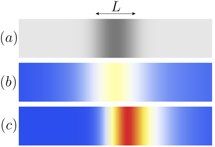
Figure 1: (a) Inhomogeneous strip with a symmetric spatial dependence of the elastic scattering rate $1/\tau(x)$ (darker region corresponds to stronger scattering). Temperature profile in the strip in the ID (b) and HD (c) regime for $l_{\rm in}=l_{*}=4L$, where $L$ is characteristic size of inhomogeneity (see the text).

II Model

We consider electron transport in a 2D system which consists of a narrow strip with an inhomogeneous distribution of the elastic scattering rate, see Figs. 1a. In this setup, the term “constriction” will be used for the region of enhanced elastic scattering (a macroscopic “defect” with increased resistance). As we will see, dissipation in this model is qualitatively similar to that in a geometric constriction with homogeneous disorder. At the same time, the disorder-controlled constriction model allows one to simplify the solution by formally reducing the problem to a one-dimensional one.

We assume a parabolic dispersion for electrons characterized by mass $m$ and start from kinetic equation describing the distribution of electrons over velocity $\mathbf{V}$ in the electric field characterized by the force $\mathbf{F}$:

$$\frac{\partial f}{\partial t}+\mathbf{V}\frac{\partial f}{\partial\mathbf{r}}+\frac{\mathbf{F}}{m}\frac{\partial f}{\partial\mathbf{V}}=\widehat{\rm St}f.$$ (1)

Here,

$$\widehat{\rm St}=\widehat{\rm St}_{\text{imp}}+\widehat{\rm St}_{\text{ph}}+\widehat{\rm St}_{\text{ee}}$$

is the collision integral including contributions from impurity, electron-phonon and electron-electron scattering, respectively. We write the impurity collision integral in a standard form

$$\widehat{\rm St}_{\text{imp}}f=\frac{f_{0}-f}{\tau},$$ (2)

where $\tau$ is the (coordinate-dependent) momentum relaxation time, $f_{0}=\langle f\rangle$, and $\langle\cdots\rangle$ stands for averaging over velocity directions.

In order to study electron-phonon heat balance, one needs to specify the electron-phonon collision integral. The simplest model of this integral, which leads to relaxation to the Fermi distribution function with the lattice temperature $T_{0}$, reads

$$\widehat{\rm St}_{\text{ph}}f=\gamma\frac{\partial}{\partial\epsilon}\left\{\epsilon\left[f_{0}(1-f_{0})+T_{0}\frac{\partial f_{0}}{\partial\epsilon}\right]\right\},$$ (3)

where $\gamma$ is the electron-phonon scattering rate which is assumed throughout the paper to be energy-independent and small compared to the momentum relaxation rate: $\gamma\tau\ll 1$. The collision integral (3) captures basic physics of the electron-phonon energy transfer and allows for exact analytical solutions. It possesses the key properties of the electron-phonon collision integrals: it vanishes in equilibrium, conserves the total number of electrons, and does not transfer energy to $\epsilon<0$. The Fokker-Planck form of the collision integral (3) can be microscopically derived for the quasi-elastic scattering by acoustic phonons perelbook for $T\gg T_{\rm BG},$ where $T_{\rm BG}$ is the Bloch-Grüneisen temperature which determines the maximum energy transferred from electron to acoustic phonons in a collision process (in the absence of impurity-assisted “supercollisions” Song ; my-supercollisions ; levitov-resonant ).

As for the electron-electron collision integral $\widehat{\rm St}_{\text{ee}}$, we do not need an explicit expression for it and only use the fact that it preserves the total particle number, energy, and momentum. For simplicity, we characterize $\widehat{\rm St}_{\text{ee}}$ by a single electron-electron collision time $\tau_{\rm ee}$.

Since the system under the consideration is inhomogeneous along the $x$ direction, the electric field depends on the coordinate and can be written as

$$F(x)=F_{0}+\delta F(x),$$ (4)

where $\delta F(x)$ is the inhomogeneity-induced correction which should be found self-consistently by solving the Poisson’s equation. The calculations drastically simplify in the limit of infinitely strong screening, when $\delta F$ can be found from the quasineutrality condition $N\approx N_{0}=\text{const}$. In this paper, we will restrict ourselves to this limit only.

Below, we use different approaches depending on the relation between momentum relaxation time $\tau$ and time of electron-electron collision, $\tau_{\rm ee}$. For the case of fast electron-electron collisions ($\tau_{\rm ee}\ll\tau$, we use a hydrodynamic ansatz, while for slow collisions we neglect the electron-electron collision integral, assuming that the thermalization occurs solely because of the electron-phonon interaction.

The strength of overheating and the degree of dissipation asymmetry depend on the relation between characteristic lengths in the problem. Specifically, one can conveniently introduce two length scales characterizing the energy transfer in the problem. The first is the diffusive length of inelastic scattering,

$$l_{*}\sim\sqrt{D_{0}/\gamma},$$ (5)

where $D_{0}$ is the diffusion coefficient in the absence of driving electric field. The second is the drift inelastic length

$$l_{\rm in}\propto v/\gamma,$$ (6)

which is proportional to the drift velocity $v$ governed by the electric field [see Eqs. (24) and (25) below].

In Fig. 2, for simplicity, we illustrate the heating regimes in the Boltzmann case, $T_{0}\gg E_{F}$, where $E_{F}$ is the Fermi energy. In this case, $D_{0}\sim T_{0}\tau/m$. Physically, the lengths $l_{*}$ and $l_{\rm in}$ characterize inelastic scattering for weak and strong driving fields, respectively. One can introduce the “true” inelastic length $l_{*}(T)$ which in the Boltzmann case reduces to $l_{*}$ and $l_{\rm in}$ in the limiting cases:

$$l_{*}(T)\sim\sqrt{\frac{D(T)}{\gamma}}=\left\{\begin{array}[]{c}l_{*},\quad l_{\rm in}\ll l_{*}\\ l_{\rm in},\quad l_{\rm in}\gg l_{*}\end{array}\right.,$$ (7)

where $D(T)\sim T\tau/m,$ and $T$ is the temperature in the presence of the field [see Eq. (14) below].

Two panels of Fig. 2 correspond to the cases $l_{*}<L$ (Fig. 2a) and $l_{*}>L$ (Fig. 2b), where $L$ is the size of the constriction. Further, the temperature distribution strongly depends on the relation between these two field-independent lengths $L$, $l_{*}$ and the drift length $l_{\rm in}$. In total, we have six different cases of ordering of the lengths $L$, $l_{*}$ and $l_{\rm in}$, which are labeled by roman numerals from I to VI in Fig. 2.

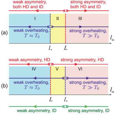
Figure 2: Schematics of dissipation regimes realized in the Boltzmann case for different relations between the field-independent lengths $l_{*}$ (diffusive electron-phonon length) and $L$ (size of the constriction) and the drift-inelastic length $l_{\rm in}$ proportional to the driving electric field. Panel (a): $L>l_{*}$, regions I, II, and III are realized with increasing $F_{0}$. Panel (b): $L<l_{*}$, regions IV, V, and VI are realized with increasing $F_{0}$.

As we show below, the difference between the HD and ID regimes is particularly pronounced in the parameter region $L<l_{\rm in}<l_{*}$ labeled V in Fig. 2b. In this case, the temperature distribution in the ID regime is almost symmetric (with overheating proportional to $F_{0}^{2}$ in accordance with earlier prediction of Ref. rokni1995joule ) and has a small ($\propto F_{0}^{3}$) asymmetric correction. The spatial size of this distribution is on the order of $l_{*}$ and thus is field-independent. By contrast, the HD temperature distribution is strongly asymmetric with the characteristic scale on the order of $l_{\rm in}$ and, therefore, can be controlled by electric field. This difference (see panels b and c of Fig. 1) can be experimentally resolved, giving a possibility to distinguish experimentally between hydrodynamic and drift-diffusion cases.

III Hydrodynamic regime

III.1 Hydrodynamic formalism

In this section, we assume that

$$\tau_{\rm ee}\ll\tau,$$ (8)

(which also implies $\tau_{\rm ee}\ll\gamma^{-1}$) so that fast electron-electron collisions drive the system into the HD regime, in which the system is fully described by local values of drift velocity, $\mathbf{v}(\mathbf{r},t)$, temperature, $T(\mathbf{r},t)$, and chemical potential $\mu(\mathbf{r},t)=N(\mathbf{r},t)/\nu$. (Here $N$ is the electron concentration and $\nu=\text{const}$ is the thermodynamic density of states.) Although the derivation of hydrodynamic equations for these quantities is quite standard and can be found in textbooks, we present this derivation in Appendix A in order to make the presentation self-contained.

The hydrodynamic heat balance equation reads

$$C\left[\frac{\partial T}{\partial t}+{\rm div}(\mathbf{v}T)\right]=N\left[\frac{mv^{2}}{\tau}-\gamma~{}(T-T_{0})\right],$$ (9)

where $C$ is the heat capacitance of a 2D system given by $C\approx{\pi^{2}\nu T}/{3}$ for $\nu T\ll N$ (Fermi distribution), and $C\approx N$ for $\nu T\gg N$ (Boltzmann distribution). In Eq. (9) we neglected the second-derivative term with the heat conductivity, which is proportional to $\tau_{\rm ee}$ in the HD limit and is, therefore, small. We will discuss the role of this term in the end of the paper.

The temperature dependence of the electron-phonon term in Eq. (9) corresponds to the collision integral (3) with energy-independent $\gamma$. Indeed, when the Fermi function with $T\neq T_{0}$ is substituted in Eq. (3), the result is proportional to $T-T_{0}$. One can generalize Eq. (9) for a more general collision integral beyond the Fokker-Planck approximation by replacing

$$\gamma\>(T-T_{0})\to\gamma\>\frac{T^{k}-T_{0}^{k}}{k\,T_{0}^{k-1}},$$ (10)

where the integer number $k$ depends on material and the type of phonons (e.g., for graphene, see Refs. Song ; my-supercollisions and references therein). Assuming that the inhomogeneity leads to a small deviation, $\delta T(x)$, of temperature from the value of $T$ at $|x|\to\infty$, linearization of collision integral yields $\gamma_{T}\delta T,$ where

$$\gamma_{T}=\gamma(T/T_{0})^{k-1}.$$

Let us make a short comment before solving Eq. (9). It was found in Ref. rokni1995joule under the assumption of electron-hole symmetry, that the temperature distribution in the overheated system is a symmetric function with respect to the current direction. As we will show below, the breaking of the particle-hole symmetry gives rise to asymmetric temperature distribution, even when the deposited heat, described by the term ${mv^{2}}/{\tau}$, is a symmetric function of $x$. The particle-hole asymmetry reveals itself in Eq. (9) through the term ${\rm div}(\mathbf{v}T)$. It is worth noting that this term is also responsible for nonzero thermopower.

Throughout the paper we will focus on calculation of the electron temperature distribution $T(x)$. What is measured in experiment is the phonon temperature $T_{0}$ which also becomes position dependent because of the energy transfer between the electron and phonon subsystems: $T_{0}\to T_{\rm ph}(x)$. This dependence can be directly found from the heat balance equation for the phonon subsystem,

$$-\kappa_{\rm ph}\Delta T_{\rm ph}=\gamma\>(T-T_{\rm ph})-\gamma_{0}\>(T_{\rm ph}-T_{0}),$$ (11)

where $\kappa_{\rm ph}$ is the phonon heat conductivity, $T_{0}=\text{const}$ is the temperature of the substrate and $\gamma_{0}$ is the rate of the heat transfer between phonon subsystem and substrate. Typically, $\gamma_{0}\gg\gamma$, and $\kappa_{\rm ph}\ll\gamma_{0}L^{2}$, so that $T_{\rm ph}$ is very close to the temperature of the substrate with a small correction which is fully expressed via the electron temperature:

$$T_{\rm ph}(x)\approx T_{0}+\frac{\gamma}{\gamma_{0}}T(x).$$ (12)

III.2 Homogeneous heating

In the stationary homogeneous case ($\partial/\partial t\to 0,\nabla\to 0$), we find from Eqs. (61), (62), and (9):

$$N=N_{0}=\text{const},\quad\frac{\mathbf{v}}{\tau}=\frac{\mathbf{F}_{0}}{m},\quad\frac{mv^{2}}{\tau}=\gamma\>(T-T_{0}),$$ (13)

yielding a homogeneous temperature of the electron system

$$T=T_{0}+\frac{F_{0}^{2}\tau}{m\gamma}$$ (14)

which differs from the substrate temperature by a conventional quadratic-in-field term. The parameter controlling the overheating is

$$\alpha=\left(1+\frac{m\gamma T_{0}}{F_{0}^{2}\tau}\right)^{-1},$$ (15)

so that

$$T=\frac{T_{0}}{1-\alpha}=\frac{F_{0}^{2}\tau}{m\gamma\alpha}.$$ (16)

For strong overheating, $1-\alpha\ll 1$, we get $T\approx{F_{0}^{2}\tau}/{m\gamma}$ and initial temperature $T_{0}$ drops out from all final equations. For a more general collision integral, we find by means of Eq. (10):

$$T=T_{0}\left(1+\frac{kF_{0}^{2}\tau}{T_{0}m\gamma}\right)^{1/k}.$$ (17)

III.3 Dissipation profile around an inhomogeneity

Next, we assume that $\tau$ depends on $x$, see Fig.1a, with a limiting value $\tau_{\infty}$ at $x\to\pm\infty$. This model can also mimick the geometrical constriction, see Appendix B. Below, we will demonstrate that even for symmetric dependence $\tau(x)=\tau(-x)$, the dependence of the temperature is asymmetric. Physically, this asymmetry arises from the electron-hole asymmetry at the Fermi level. Therefore, the effect becomes particularly strong for the Boltzmann distribution ($T\gg\mu$) for which the electron-hole asymmetry is maximal.

We focus on the simplest case of very short screening length, when quasineutrality of the electron liquid dictates its incompressibility. The corresponding criterion is most transparent for a gated system (see Appendix A) characterized by the electrical capacitance $\mathcal{C}$. The incompressible regime is effectively realized when the plasma-wave velocity $s=\sqrt{{e^{2}N_{0}}/{m\mathcal{C}}}$ is sufficiently large: $s^{2}\gg T/m.$ In this regime, putting in Eq. (62)

$$N\approx N_{0}=\text{const}$$ (18)

and using then the current conservation,

$$v=|\mathbf{v}|\approx\frac{F_{0}\tau_{\infty}}{m}=\text{const},$$ (19)

one simplifies Eq. (9):

$$Cv\frac{dT}{dx}=N_{0}\left[\frac{mv^{2}}{\tau(x)}-\gamma\>\frac{T^{k}-T_{0}^{k}}{kT_{0}^{k-1}}\right],$$ (20)

where $C\approx C(N_{0},T)$.

The temperature of the electron gas at $|x|\to\infty$ is given by Eq. (17) with the replacement $\tau\to\tau_{\infty}$. For strong field, $T$ can be much larger than $T_{0}$. For weak inhomogeneities, one can linearize collision integral around $T$. Let us assume that $\tau$ has a small $x$-dependent correction and introduce the dimensionless function

$$\xi(x)=\frac{\tau_{\infty}}{\tau(x)}-1=\int\frac{dq}{2\pi}e^{iqx}\xi_{q},\quad\xi(x)\ll 1,$$ (21)

Then, Eq. (20), linearized with respect to $\xi$, becomes

$$\frac{d\delta T}{dx}+\frac{\delta T}{l_{\rm in}}=G(x),$$ (22)

where $\delta T=T(x)-T$,

$$G(x)=\frac{F_{0}N_{0}}{C}\xi(x),$$ (23)

and

$$l_{\rm in}=\frac{C}{N_{0}}\frac{v}{\gamma_{T}}$$ (24)

is the drift inelastic length with $v$ given by Eq. (19). The latter simplifies for the Boltzmann case (where $C\approx N_{0}$) and for a simplified collision integral (3) for which $k=1$ and $\gamma_{T}=\gamma$:

$$l_{\rm in}=\frac{v}{\gamma}.$$ (25)

Solution of Eq. (22) reads

$$\delta T(x)=\int\limits_{-\infty}^{\infty}dx^{\prime}K(x-x^{\prime})G(x^{\prime}),$$ (26)

where

$$K(x)=\int\frac{dq}{2\pi}\frac{e^{iqx}}{iq+1/l_{\rm in}}=\theta(x)e^{-x/l_{\rm in}}$$ (27)

is strongly asymmetric function of $x$.

The temperature profile (26) is shown in Fig. 3 for several values of $L/l_{\rm in}$. For convenience, we assumed a Gaussian shape of the inhomogeneity $1/\tau(x)$ formula . It is seen from the figure that the asymmetry is very strong in the limit $L/l_{\rm in}\ll 1$ and becomes weak in the opposite limit. Below we analyze analytically these two limiting cases.

For weak coupling to the phonon system,

$$L\ll l_{\rm in},$$ (28)

the shape of the function $\delta T(x)$ is strongly asymmetric: it decays for $x<0$ within the distance $L$ and within much longer distance $l_{\rm in}$ for $x>0$. In the limit $l_{\rm in}=\infty$, a maximum asymmetry is reached and the difference of temperatures at $x=\pm\infty$ tends to a finite value:

$$\delta T_{\rm max}=\frac{F_{0}N_{0}}{C}\int\limits_{-\infty}^{\infty}\xi(x)dx,$$ (29)

Hence, the asymmetric part of the temperature distribution is proportional to the first power of the driving force $F_{0}$ and remains finite in the limit $l_{\rm in}\to\infty$ (for a fixed system size). Fixing $l_{\rm in}$ and turning $L\to 0$, we find

$$\delta T(x)\approx\delta T_{\rm max}K(x).$$ (30)

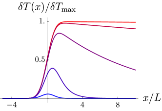
Figure 3: Spatial dependence of temperature in the HD regime for fixed $L$ and different $l_{\rm in}$. From top to bottom: $L/l_{\rm in}=0.001,0.01,0.1,1,$ and $10.$ Dependence $\tau(x)$ is modeled by the Gaussian shape with the width determined by $L$: ${1}/{\tau(x)}=\left({1}/{\tau_{0}}-{1}/{\tau_{\infty}}\right)\exp(-{x^{2}}/{L^{2}})+{1}/{\tau_{\infty}}$ formula .

In the opposite limit of fast electron-phonon collisions, $L\gg l_{\rm in}$, the assymetry is weak. The temperature can be found by expanding $G(x^{\prime})$ in the Taylor series near $x^{\prime}=x$ in Eq. (26). This yields

$$\delta T(x)\approx l_{\rm in}G(x)-l_{\rm in}^{2}\frac{dG(x)}{dx}.$$ (31)

The asymmetry is encoded in the second term which, for the Fokker-Planck collision integral (3), is proportional in the Boltzmann case to $(F_{0}^{3}/\gamma^{2})d\tau(x)/dx$, as follows from Eqs. (25), (19), (23), and (21). Hence, for weak electrical driving, the asymmetry arises in the third order with respect to electric field. With increasing field, the asymmetry becomes proportional to $F_{0}$ as follows from Eq. (29). This explains why this asymmetry is not captured by a conventional perturbative-in-field approach which accounts for heating effects within quadratic-in-field approximation rokni1995joule (see a more detailed discussion in Sec. V).

It is instructive to analyze how increasing the chemical potential (and thus decreasing degree of the electron-hole asymmetry) affects the dissipation regime. For large $\mu$, we have $l_{\rm in}\propto C/N\sim T/\mu$. Therefore, for sufficiently large chemical potential, $l_{\rm in}$ becomes smaller than $L$ and we drive the system into regime of weak asymmetry described by Eq. (31).

To conclude this Section, we would like to stress that within the hydrodynamic picture, inhomogeneity of overheating is only controlled by the relation between the size of the resistance inhomogeneity $L$ and drift inelastic length $l_{\rm in}$, as illustrated in Fig. 2. Parameter regions I, II, and IV correspond to weak asymmetry of dissipation, while in the regions III, V, and VI the asymmetry is relatively strong.

IV Impurity-dominated regime

IV.1 Kinetic equation formalism and general solution

In the previous Section, we discussed the hydrodynamic limit, assuming that the momentum-conserving electron-electron collision time is the shortest scattering time. Let us now consider the opposite case of dominating impurity scattering:

$$1/\tau\gg\gamma\gg 1/\tau_{\rm ee},$$ (32)

when the electron-electron collision integral can be neglected. For simplicity, we will restrict ourselves to the non-degenerate (Boltzmann) regime and assume that the momentum-relaxation time is independent of energy. We will also rely on the model form of the collision integral Eq. (3). Such a model allows for exact analytical solution.

We search for solution to Eq. (1) in the standard form (see, e.g., Ref. rokni1995joule )

$$f=f_{0}(\mathbf{r},\epsilon)+f_{1}(\mathbf{r},\epsilon)e^{i\theta}+f_{-1}(\mathbf{r},\epsilon)e^{-i\theta},$$ (33)

where $\theta$ is the angle of velocity $\mathbf{V}$ and $\epsilon=mV^{2}/2$ is the particle energy. The neglect of higher angular harmonics $f_{n}$ with $|n|>1$ is justified provided that $\tau$ is the shortest time scale, such that elastic mean free path is shorter than both inhomogeneity size $L$ and inelastic length $l_{*}(T)$ given by Eq. (7).

Substituting Eq. (33) into Eq. (1), projecting thus obtained equation onto $0$ and $\pm 1$ angular harmonics, we get a closed set of equations for $f_{0},f_{1}$ and $f_{-1}.$ Next, expressing $f_{\pm 1}$ through $f_{0}$, we derive a closed equation for the isotropic part of the distribution function

$$-\left(\frac{\partial}{\partial x}+F\frac{\partial}{\partial\epsilon}\right)D(\varepsilon)\left(\frac{\partial}{\partial x}+F\frac{\partial}{\partial\epsilon}\right)f_{0}=\widehat{\rm St}_{\rm ph}\,f_{0},$$ (34)

where $D(\epsilon)=\epsilon\tau/m$ is the energy-dependent diffusion coefficient.

For the homogeneous system $\tau(x)\equiv\tau$ one has

$$-F_{0}^{2}\frac{\partial}{\partial\epsilon}D(\varepsilon)\frac{\partial}{\partial\epsilon}f_{0}(\epsilon)=\widehat{\rm St}_{\rm ph}~{}f_{0}.$$ (35)

For the model collision integral given by Eq. (3), the solution of Eq. (35) gives the Boltzmann distribution

$$f_{T}=\nu N_{0}\exp(-\epsilon/T)$$

with the temperature given by Eq. (14). For an inhomogenous system, we search for a solution to Eq. (34) by expanding $f_{0}$ in $\xi$ (see Eq. 21). To this end, we write

$$f_{0}=f_{T}+\delta f,$$ (36)

where $\delta f\propto\xi$ is a small inhomogeneity-induced correction. We linearize Eq. (34) with respect to $\delta f$, $\xi(x)$ and

$$\lambda(x)=\delta F(x)/F_{0}$$ (37)

where

$$\delta F(x)=-\frac{e^{2}}{\mathcal{C}}\nabla\delta N$$ (38)

is the electrostatic force induced by the density variation $\delta N=\nu\int d\epsilon\delta f$ (see Appendix A).

The kinetic equation linearized with respect to $\delta f$ acquires the form

$$\hat{L}\delta f=\mathcal{S},$$ (39)

where $\hat{L}$ is a linear operator and $\mathcal{S}$ is an energy-dependent source. Exact expressions for $\hat{L}$ and $\mathcal{S}$ are given in Appendix C. Interestingly, the operator $\hat{L}$ is non-Hermitian but has a discrete spectrum, which stems from the requirement that the distribution function should be finite both at zero energy (one of the solutions is logarithmically divergent at $\epsilon\to 0$) and at $\epsilon=\infty$ (one of the solutions grows exponentially at $\epsilon\to\infty$).

The explicit solution of Eq. (39) is presented in terms of the eigenmode expansion in Appendix C. The final result for the temperature distribution

$$\delta T(x)=\int_{0}^{\infty}\left(\frac{\epsilon}{T}-1\right)\delta f\left(x,\epsilon\right)d\epsilon$$ (40)

can be written in the form analogous to Eqs. (26) and (23), with the Fourier transform of the kernel given by Eq. (81) in Appendix C. Let us now discuss various limiting cases of this kernel. To this end, we introduce the field-independent length

$$l_{*}=\sqrt{\frac{T_{0}\tau_{\infty}}{m\gamma}},$$ (41)

which has a physical meaning of the diffusive energy relaxation length in weak fields when overheating can be neglected, i.e.

$$\alpha\approx\frac{F^{2}\tau_{\infty}}{m\gamma T_{0}}\ll 1\qquad\textrm{ and }\qquad T\approx T_{0}.$$ (42)

The length $l_{*}$ was denoted $\tilde{l}$ in Ref. rokni1995joule . For small $\alpha$, we have $l_{\rm in}=\sqrt{\alpha}l_{*}$. Further consideration depends on the relation between $l_{*}$ and $L$, as shown in Figs. 2(a) and (b) for $L>l_{*}$ and $L<l_{*}$, respectively. Let us now discuss possible limiting cases.

IV.2 Large defect size

At large $L$, the size of the macroscopic defect is the largest scale: $L\gg l_{\rm in},l_{*}$. This situation corresponds to the regions I and II in Fig. 2(a). In this case dissipation is almost local, the asymmetry is weak and $\delta T(x)$ is determined by local Joule heat with small non-local corrections. Technically, analytical expression for $\delta T$ can be found by expanding the Fourier-transformed dissipation kernel (81) into series over the wave-vector. In order to find this expansion up to the third order in gradients $\partial_{x}$, it is enough to cut the sums in Eq. (81) at $n=2$ and $m=1$ and replace in these sums $Q$ with $-i\partial_{x}.$ As a result, we find

$$\delta T(x)\approx F_{0}l_{\rm in}\hat{\mathcal{K}}_{0}\xi(x)$$ (43)

with

$$\hat{\mathcal{K}}_{0}=1-l_{\rm in}\partial_{x}+\left(1+\frac{2}{\alpha}\right)l_{\rm in}^{2}\partial_{x}^{2}-\left(1+\frac{8}{\alpha}\right)l_{\rm in}^{3}\partial_{x}^{3}$$ (44)

and $\xi$ given by Eq. (21).

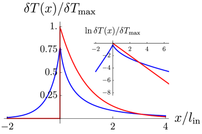
Figure 4: Spatial dependence of temperature in the hydrodynamic (red curve) and impurity-dominated (blue curve) regimes for the case $l_{\rm in}\gg L,\>l_{*}$ (regions III and VI in Fig. 2).

IV.3 Large field

At large $F$, the field-related scale $l_{\rm in}$ is the largest one: $l_{\rm in}\gg L,l_{*}$. This situation corresponds to the regions III and VI in Fig. 2. The overheating is strong in this case ($\alpha=1$) and $T\gg T_{0}$. The defect can be treated as point-like and, as a result, $\delta T(x)/T$ is a universal function of $x/l_{\rm in}$. This function is plotted in Fig. 4 by the blue line. It is interesting to note that $\int\delta T(x)dx$, as well as $\int x\delta T(x)dx$ are the same for the hydrodynamic and impurity-dominated regimes.

IV.4 Small field

At small $F$, when $l_{\rm in}\ll l_{*}$, the dissipation kernel $\hat{\mathcal{K}}$ relating $\delta T(x)$ and $\xi(x)$ can be expanded in $F$. In this case, overheating is small and characteristic inelastic length is given by $l_{*}$ [see Eq. (7)]. This situation corresponds to the regions I, IV, and V in Fig. 2. Keeping the two leading terms in the expansion over $F$, we may write

$$\delta T(x)=F_{0}l_{\rm in}\left[\hat{\mathcal{K}}_{s}+\frac{Fl_{*}}{T}\hat{\mathcal{K}}_{a}\right]\xi(x),$$ (45)

where $\hat{\mathcal{K}}_{s,a}$ are non-local integral operators with spatial scale $l_{*}$:

$$\hat{\mathcal{K}}_{s,a}\,\xi(x)=l_{*}^{-1}\int K_{s,a}\left(\frac{x-x^{\prime}}{l_{*}}\right)\xi(x^{\prime})dx^{\prime}.$$ (46)

Kernels $K_{s}$ and $K_{a}$ are even/odd functions with respect to their argument, respectively. Evaluation of these kernels requires calculation of the sums in Eq. (81). Although they can be explicitly evaluated in terms of hypergeometric functions, the result is too cumbersome to be presented here. Instead, we plot these kernels in Fig. 5.

Assuming further that $L\ll l_{*}$, we find for the regions IV and V of Fig. 2:

$$\delta T(x)=\frac{l_{\rm in}}{l_{*}}\delta T_{\rm max}\left[K_{s}\left(\frac{x}{l_{*}}\right)+\frac{l_{\rm in}}{l_{*}}K_{a}\left(\frac{x}{l_{*}}\right)\right]$$ (47)

with

$$\delta T_{\rm max}=F_{0}\int dx\,\xi(x).$$ (48)

The symmetric term is proportional to $F_{0}{l_{\rm in}}/{l_{*}}\propto F^{2}$ and gives non-local symmetric overheating. An analogous contribution to $\delta T(x)$ was found in Ref. rokni1995joule in the relaxation time approximation for the electron-phonon collision integral. Non-locality effects are controlled by the diffusive inelastic length $l_{*}$, in accordance with results of Ref. rokni1995joule . The asymmetric term in Eq. (47) is proportional to $F_{0}^{3}$. It gives correction which is small in $l_{\rm in}/l_{*}$ in this regime, and, therefore, leads to a weak asymmetry of the temperature distribution. This term is beyond the $F_{0}^{2}-$approximation used in Ref. rokni1995joule .

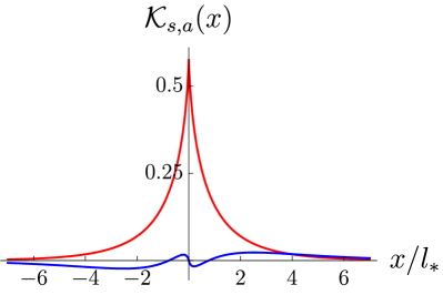
Figure 5: Spatial dependence of kernels $K_{s}$ (red curve) and $K_{a}$ (blue curve), Eq. (46).

IV.5 Overlap of “large-defect” and “small-field” regimes

Equations (43) and (45) have a certain overlap in validity: region I. In particular, considering Eq. (43) in the limit of small overheating $\alpha\to 0$ and considering Eq. (45) in the local limit $l_{*}\ll L$, when

$$\hat{\mathcal{K}}_{s}=1+2l_{*}^{2}\partial_{x}^{2},\qquad\hat{\mathcal{K}}_{a}=-l_{*}\partial_{x}-8l_{*}^{3}\partial_{x}^{3},$$

we arrive to the same expression:

$$\delta T(x)\!\approx\!F_{0}l_{\rm in}\left[\left(1+2l_{*}^{2}\partial_{x}^{2}\right)\!-l_{\rm in}\!\left(\partial_{x}+8l_{*}^{2}\partial_{x}^{3}\right)\right]\xi(x).$$ (49)

V Comparison of hydrodynamic and impurity-dominated regimes

Let us now compare the results obtained in the HD and ID limits. In the large-field regime corresponding to regions III and VI in Fig. 2, the hydrodynamic temperature distribution looks rather simple. Indeed, in this case, the function $\xi(x)$ is sharply peaked as compared to the inelastic length $l_{\rm in}$ and, as a result [see Eq. (27)],

$$\delta T=\delta T_{\rm max}\theta(x)\exp(-x/l_{\rm in}),$$ (50)

with $\delta T_{\rm max}$ given by Eq. (48) for the Boltzmann case ($C=N_{0}$). We plot this dependence in Fig. 4 together with the corresponding dependence obtained in the ID strongly overheated regime ($\alpha=1$). We see that the hydrodynamical function is much more asymmetric. One of the physical reasons for this difference is that electron-electron collisions suppress heat conductivity, which turns out to be proportional to $\tau_{\rm ee}$ and turns to zero in the purely hydrodynamical limit of ideal fluid, $\tau_{\rm ee}\to 0$.

Let us now discuss what happens if we take into account small corrections with respect to $\tau_{\rm ee}$ allowing for a finite heat conductivity, $\kappa_{0}\neq 0$, of the electron fluid. This modifies Eq. (22) as follows:

$$\frac{d\delta T}{dx}-\rho\frac{d^{2}\delta T}{dx^{2}}=G(x)-\frac{\delta T}{l_{\rm in}},$$ (51)

where

$$\rho=\frac{\kappa_{0}}{Cv}$$ (52)

Solution of Eq. (51) is given by Eq. (26) with

$$K(x) = \int\limits_{-\infty}^{\infty}\frac{dq}{2\pi}\frac{e^{iqx}}{iq+1/l_{\rm in}+\rho q^{2}}$$ (53)

$$= \int\limits_{0}^{\infty}\frac{dt}{2\sqrt{\pi\rho t}}\exp\left[-\frac{t}{l_{\rm in}}-\frac{(x-t)^{2}}{4t\rho}\right].$$

Analyzing Eq. (53), we find that the heat conductivity does not affect the shape of the temperature distribution and can, therefore, be fully neglected provided that

$$\rho\ll L,$$

or, equivalently ${CvL}/{\kappa_{0}}\gg 1.$ For $L\ll\rho\ll l_{\rm in}$ the sharp jump in the temperature distribution at $x=0$ (see Fig. 3) gets broadened but the distribution is still asymmetric. Only for $\rho\gg l_{\rm in}$ the asymmetry starts to decrease.

For $l_{*}\ll L$ and low field $l_{\rm in}\ll L$ [regions I and II in Fig. 2(a)], the temperature correction can also be found by expanding the Fourier transform of the hydrodynamic kernel $K(x)$ [see Eqs. (26) and (27)] into series over $q$. Then, we obtain:

$$\delta T^{\rm hydro}(x)\approx F_{0}l_{\rm in}\left[1-l_{\rm in}\partial_{x}+l_{\rm in}^{2}\partial_{x}^{2}-l_{\rm in}^{3}\partial_{x}^{3}\right]\xi.$$ (54)

Comparing this formula with Eq. (43), we conclude that the hydrodynamic temperature distribution, in contrast to impurity-dominated one, is not sensitive to the overheating parameter. This happens because in the hydrodynamic regime diffusive heat transfer is suppressed and the only relevant scale for energy relaxation is the drift energy relaxation length $l_{\rm in}.$

The difference between HD and ID heating is most pronounced in region V in Fig. 2(b). Here, the impurity-dominated overheating, described by the first term in Eq. (47), is almost symmetric (with weak anisotropic correction $\propto K_{\rm as}$), and is dimensionless function of $x/l_{*},$ while hydrodynamic overheating is strongly asymmetric and is given by a dimensionless function of $x/l_{\rm in}$ [see Eq. (50)]. It is worth noting that such two dependencies can be easily distinguished experimentally because $l_{\rm in}$ is field-dependent in contrast to $l_{*}$.

To characterize the degree of asymmetry of the dissipation, we define the corresponding dimensionless visibility

$$\mathcal{V}=\frac{\int_{0}^{\infty}\delta T(x)dx-\int_{-\infty}^{0}\delta T(x)dx}{\int_{-\infty}^{\infty}\delta T(x)dx}.$$

In Fig. 6 we show the crossover in the visibility from the hydrodynamic to the impurity-dominated regime for the case of a small defect, $L\ll(l_{*},l_{\rm in})$. In the ideal hydrodynamic limit, $\tau_{ee}\to 0$ ($\rho=0$), the visibility is simply given by unity. For the hydrodynamics with a finite heat conductivity, the analytical expression for visibility is given by

$$\mathcal{V}=\left(1+\frac{4\rho}{l_{\rm in}}\right)^{-1/2}$$ (55)

In order to evaluate $\rho$ defined in Eq. (52), we estimate the heat conductivity $\kappa_{0}$ in the HD regime as $\kappa_{0}\sim(\tau_{\rm ee}/\tau)CD$. It follows that

$$\rho=\frac{T}{T_{0}}\left(\tau_{\rm ee}/\tau\right)l_{*}^{2}/l_{\rm in}.$$

Using now

$$l_{*}/l_{\rm in}=\sqrt{{1}/{\alpha}-1},$$ (56)

where $\alpha$ is a dimensionless parameter defined in Eq. (15), we find

$$\mathcal{V}=\frac{\sqrt{\alpha}}{\sqrt{\alpha+{4\tau_{\rm ee}}/{\tau}}}.$$ (57)

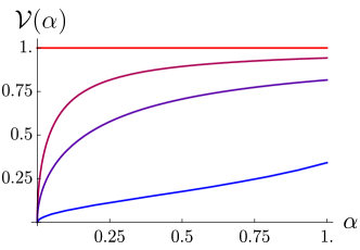
Figure 6: Visibility of the asymmetry, $\mathcal{V}$ for a small inhomogeneity [$L\ll l_{\rm in},$ regions III, V and VI in Fig. 2 (b)] as a function of the parameter $\alpha$ defined in Eq. (56). For the electron-phonon collision integral as in Eq. (9), i.e., with $k=1$, the parameter $\alpha$ is given explicitly by Eq. (15). The limits $\alpha\to 0$ and $\alpha\to 1$ correspond then to weak and strong field, respectively. Upper line (red) – hydrodynamic regime, $\tau_{\rm ee}/\tau\to 0$; visibility is maximal (equal to unity). Lower line (blue) – impurity-dominated regime, $\tau_{\rm ee}/\tau\to\infty$, calculated by using the results of Sec. IV.1 and Appendix C. Intermediate curves illustrate the crossover between the hydrodynamic and impurity-dominated limits, as described by Eq. (57); they correspond to $\tau_{\rm ee}/\tau=0.125$ and 0.5.

In the impurity-dominated regime, the visibility is calculated by using the results for the spatial profile of temperature in Sec. IV.1 and Appendix C. The corresponding asymptotic behavior of the visibility in the case of weak field (small $\alpha$) can be found from Eq. (47). The result is expressed in terms of the odd and even kernels (Fig. 5) as

$$\mathcal{V}=\sqrt{\alpha}\ \dfrac{\int_{0}^{\infty}K_{a}(x)dx}{\int_{0}^{\infty}K_{s}(x)dx}\approx 0.21\sqrt{\alpha}.$$ (58)

Finally, we remind the reader that the formula (15) for the parameter $\alpha$ was derived for a particular form of the electron-phonon collision integral, as in Eq. (9), which corresponds to $k=1$. The results derived above have, however, a general validity when expressed in terms of the relevant length scales. For a general collision integral, Eq. (10), we find from Eqs. (26) and (24)

$$l_{\rm in}=\frac{CF_{0}\tau}{\gamma N_{0}m}\frac{1}{\left(1+\frac{kF_{0}^{2}\tau}{T_{0}m\gamma}\right)^{(k-1)/k}}.$$ (59)

The results shown in Fig. 6 remain valid, with $\alpha$ defined now by Eq. (56) and with $l_{\rm in}$ from Eq. (59). Note that for $k>2$ the length $l_{\rm in}$ becomes a non-monotonous function of the electric field.

VI Summary

To summarize, we have investigated dissipation in a narrow constriction in a two-dimensional electron system. Our main prediction is a rather strong current-induced asymmetry in the heating of the electron and phonon systems, which is different in hydrodynamical and impurity-dominated regimes. The spatial profile of the dissipation in the hydrodynamic regime turns out to exhibit a particularly strong asymmetry, as illustrated in Fig. 1. The corresponding spatial scale of the temperature distribution, $l_{\rm in}$, can be controlled by the driving field. By contrast, the asymmetry of impurity-dominated heating is moderate, and the spatial scale of corresponding temperature distribution, $l_{*}$, does not depend on the field. The degree of the asymmetry is controlled by the parameter $\alpha$ that depends on the strength of the applied electric field, see Fig. 6. Our results are consistent with recent experimental findings on dissipation in narrow constrictions and quantum point contacts.

As further developments of our study, it would be worth considering other geometries (including point contacts), the effects of magnetic field, as well as effects of viscosity and boundary scattering in the hydrodynamic regime.

VII Acknowledgments

We are grateful to E. Zeldov for motivating discussions and sharing the unpublished experimental data with us. We also acknowledge collaboration with K. Dapper at the early stage of the work. We thank G. Zhang for carefully reading the manuscript and useful comments. This work is supported by the program 0033-2019-0002 by the Ministry of Science and Higher Education of Russia, by the FLAGERA JTC2017 Project GRANSPORT through the DFG Grant No. GO 1405/5, by RFBR (Grant No. 17-02-00217), by Foundation for the Advancement of Theoretical Physics and Mathematics “BASIS”, and by the Foundation for Polish Science through the grant MAB/2018/9 for CENTERA. KT acknowledges support by Alexander von Humboldt Foundation.

Appendix A Derivation of hydrodynamic equations

In this Appendix, we provide a derivation of the hydrodynamic equations used in Sec. III. We search for solution in the form of hydrodynamic ansatz

$$f(\mathbf{r},\mathbf{V})=\dfrac{1}{\exp\left\{\dfrac{m\left[\mathbf{V}-\mathbf{v}(\mathbf{r},t)\right]^{2}/2-\mu(\mathbf{r},t)}{T(\mathbf{r},t)}\right\}+1},$$ (60)

where $\mathbf{v}(\mathbf{r},t),\ T(\mathbf{r},t)$, and $\mu(\mathbf{r},t)=N(\mathbf{r},t)/\nu,$ are, respectively, local values of drift velocity, temperature and chemical potential, $N$ is the electron concentration and $\nu=\text{const}$ is the thermodynamic density of states. Multiplying Eq. (1) by “$1$”, “$\mathbf{V}$’, and“$\epsilon=mV^{2}/2$”, integrating over $\mathbf{V}$ and using ansatz (60), after some algebra, we get the following set of equations:

$$\!\!\frac{\partial N}{\partial t}+{\rm div}\left(\mathbf{v}N\right)=0,$$ (61)

$$\!\!\frac{\partial\mathbf{v}}{\partial t}+(\mathbf{v}\nabla)\mathbf{v}+\frac{\mathbf{v}}{\tau}=\frac{1}{m}\left(\mathbf{F}_{0}-\frac{e^{2}\nabla N}{\cal C}-\frac{1}{N}\nabla W\right),$$ (62)

$$\!\!\frac{\partial W}{\partial t}+{\rm div}\left(\mathbf{v}W\right)+W{\rm div}\mathbf{v}=N\left[\frac{mv^{2}}{\tau}-\gamma(T-T_{0})\right],$$

(63)

where $\mathbf{F}_{0}$ is driving electric force in the homogeneous case, $-{e^{2}\nabla N}/{\cal C}$ is inhomogeneity-induced correction to this force, ${\cal C}$ is the gate-to-channel capacitance per unit length (we assume that the system is gated), and

$$W=W(N,T)=\int_{0}^{\infty}d\epsilon\epsilon f_{F}(\epsilon)$$

is the density of energy in the moving frame (here $f_{F}=1/\exp[(\epsilon-\mu)/T+1]$ is the Fermi function and $\mu=T\ln\left[\exp(N/\nu T)-1\right]$), which is given by

$$W=\left\{\begin{array}[]{c}\displaystyle\frac{N^{2}}{2\nu}+\frac{\pi^{2}\nu T^{2}}{6},\quad{\rm for}~{}\nu T\ll N{}\\ \\ \displaystyle TN,\quad{\rm for}~{}\nu T\gg N.\end{array}\right.$$ (64)

Here, we neglected the heat conductivity and viscosity of the electron liquid, setting $\tau_{\text{ee}}\to 0$.

Introducing heat capacitance

$$C=C(N,T)=(\partial W/\partial T)_{N=\text{const}}$$

after some algebra we obtain from Eqs. (61),(62), and (63), the temperature balance equation Eq. (9), of the main text.

Appendix B Smooth constriction

In this Appendix, we demonstrate that the results obtained for the hydrodynamic regime obtained in Sec. III for a model of $\tau(x)$ inhomogeneity are in fact generic and hold also for a constriction. Specifically, we assume that the width of the strip smoothly varies, forming a geometric constriction characterized by the local strip width $a(x)$, see Fig. 7. Such a constriction works effectively as an additional source of local resistance, so that even for $\tau(x)=\text{const}$ the temperature is expected to vary along the strip. This setup can be viewed as a prototype of a point contact considered in Ref. rokni1995joule . For incompressible electron fluid, we still assume $N\approx N_{0}=\text{const}$. Then, because of the total current conservation, the current density and, hence, the drift velocity become $x$-dependent:

$$v(x)=v_{\infty}\frac{a_{\infty}}{a(x)},$$ (65)

where $v_{\infty}=F_{0}\tau_{\infty}/m.$

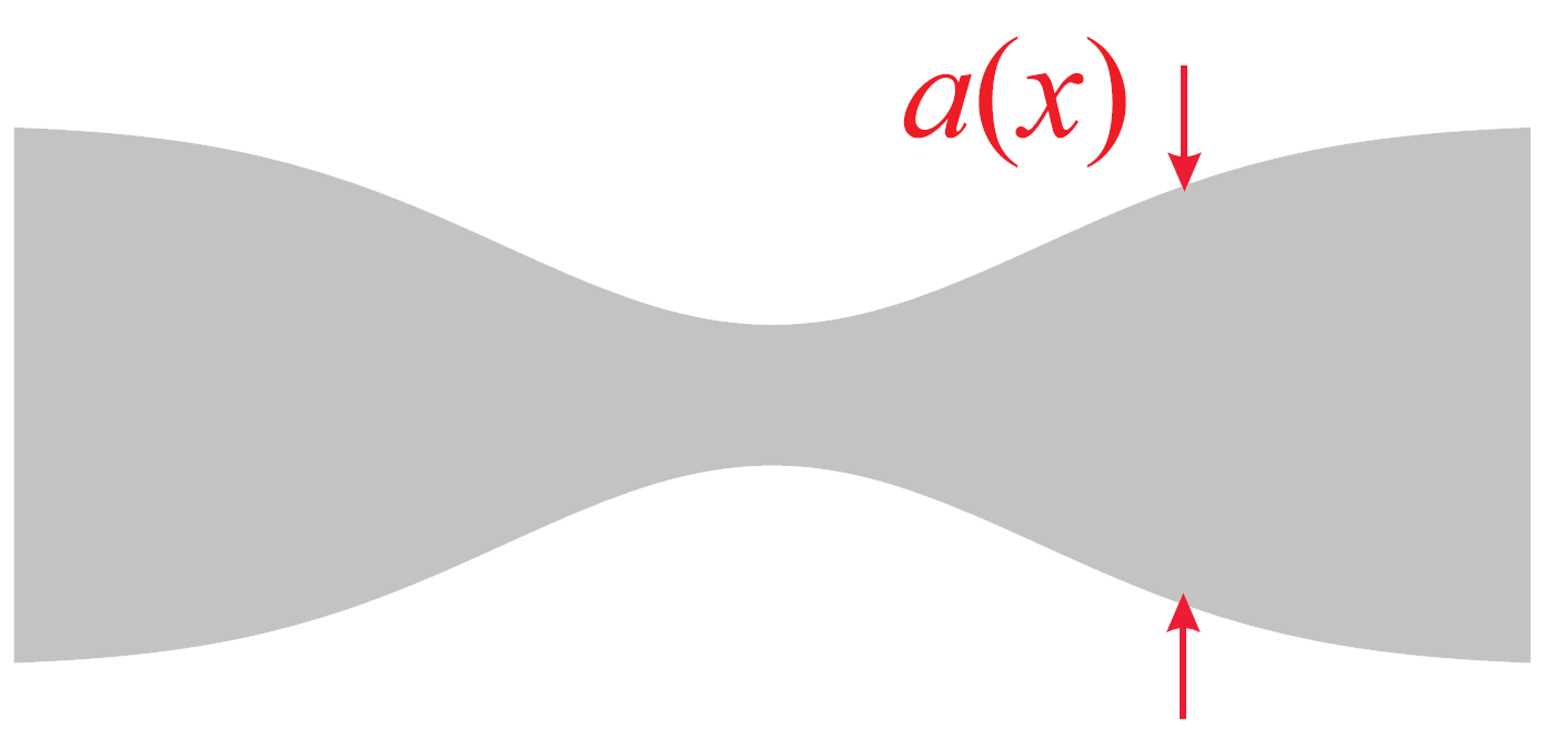
Figure 7: Schematics of a smooth constriction.

Assuming that $|T(x)-T|\ll T,$ we linearize Eq. (10) with respect to small variation of $T(x)$ $v(x)$ and $\tau(x).$ In the absence of variations, Eq. (10) is satisfied because of the identity [see Eq. (13)]

$$m\frac{v_{\infty}}{\tau_{\infty}}=\frac{\gamma}{v_{\infty}}(T-T_{0}),$$ (66)

which relates $v_{\infty}$ and $T=T(x\to\pm\infty).$ In the first order, we get

$$\frac{C}{N_{0}}\left(\frac{d\delta T}{dx}+\frac{T}{v_{\infty}}\frac{dv}{dx}\right)$$ (67)

$$=m\left(\frac{v}{\tau}-\frac{v_{\infty}}{\tau_{\infty}}\right)-\frac{\gamma}{v_{\infty}}\delta T-\gamma\,(T-T_{0})\left(\frac{1}{v}-\frac{1}{v_{\infty}}\right).$$

Expressing $T-T_{0}$ in the last term in the r.h.s. of this equation with the use of Eq. (66), we find that Eq. (22) is still valid with a minor modification of $G(x)$:

$$G(x)=\frac{mN_{0}}{C}\left[\frac{v(x)}{\tau(x)}-\frac{v_{\infty}^{2}}{\tau_{\infty}v(x)}\right]-\frac{T}{v_{\infty}}\frac{dv}{dx}.$$ (68)

Now, Eq. (26) is valid with $G(x)$ given by Eq. (68). As a result, for $\tau=\text{const}$ we find

$$\delta T_{\rm max}=\frac{F_{0}N_{0}}{C}\int\limits_{-\infty}^{\infty}dx\left[\frac{a_{\infty}}{a(x)}-\frac{a(x)}{a_{\infty}}\right]$$ (69)

which is analogous to Eq. (29).

Appendix C Solution of the kinetic equation in the impurity-dominated limit

In this Appendix, we solve the linearized kinetic equation (34) for $\delta f$ defined in Eq. (36). Using dimensionless variables

$$E=\epsilon/T,\quad X=x/l_{\rm in},\quad Q=ql_{\rm in},$$

where $l_{\rm in}=v/\gamma$ with $v$ given by Eq. (19), we find the following equation for the Fourier transform $\delta f_{Q}$ of $\delta f(x)$ introduced in Eq. (36):

$$\hat{L}\delta f_{Q}=\xi_{Q}S_{1}\left(E\right)+\lambda_{Q}S_{2}\left(E\right).$$ (70)

Here

$$\hat{L}=E\partial^{2}_{E}+\left(2iQE+E+1\right)\partial_{E}+1+iQ-\frac{Q^{2}E}{\alpha}$$ (71)

and

$$S_{1}\left(E\right)=e^{-E}\left(\alpha E-iQE-\alpha\right),$$ (72)

$$S_{2}\left(E\right)=e^{-E}\left(2\alpha E-2\alpha-iQE\right).$$ (73)

The parameter $\alpha$ characterizes the degree of overheating [see Eq. (15)]. The function $\lambda_{Q}$ entering the right-hand side of Eq. (70) should be found self-consistently with the use of Eqs. (37) and (38).

The requirement that the distribution function is finite both at $E=0$ (where one of the solutions diverges logarithmically) and at $E=\infty$ (where one of the solutions diverges exponentially) gives rise to discrete spectrum of the operator $\hat{L}$. Eigenfunctions $f_{n}$ and eigenvalues $L_{n}$ of the operator $\hat{L}$ enumerated by integer index $n=0,1,2,\ldots$ read

$$f_{n}\left(E\right)=e^{-\frac{1}{2}\left(1+2iQ+Z\right)E}U\left(-n,1,ZE\right),$$ (74)

$$L_{n}=\frac{1}{2}\left(1-Z-2nZ\right),$$ (75)

where

$$Z=\sqrt{1+4Q\left[i+Q\left(1/\alpha-1\right)\right]}$$

and $U(a,b,z)$ is the confluent hypergeometric function (polynomial in $z$ at negative integer $a$). The functions $f_{n}\left(E\right)$ obey orthogonality condition

$$\int_{0}^{\infty}f_{m}\left(E\right)f_{n}\left(E\right)e^{E\left(1+2iQ\right)}dE=\frac{\left(n!\right)^{2}}{Z}\delta_{mn}.$$

Now, we can solve Eq (70) by the eigenmode expansion:

$$\delta f_{Q}\left(E\right)=\sum_{n=0}^{\infty}\left[\xi_{Q}A_{n}^{\left(1\right)}+\lambda_{Q}A_{n}^{\left(2\right)}\right]f_{n}\left(E\right)$$ (76)

where for $k=1,2$

$$A_{n}^{\left(k\right)}=\frac{1}{L_{n}}\frac{Z}{\left(n!\right)^{2}}\int_{0}^{\infty}S_{k}\left(E\right)f_{n}\left(E\right)e^{E\left(1+2iQ\right)}dE.$$ (77)

We may now evaluate $\lambda_{Q}$. We limit ourselves with electroneutral limit $e\to\infty$, where the corresponding condition becomes $\delta N=0$. In this limit, we find

$$\lambda_{Q}=-\frac{\sum_{n=0}^{\infty}A_{n}^{\left(1\right)}N_{n}}{\sum_{n=0}^{\infty}A_{n}^{\left(2\right)}N_{n}}\xi_{Q}.$$ (78)

where

$$N_{n}=\int_{0}^{\infty}f_{n}\left(E\right)dE.$$

Finally, we calculate the effective temperature of the distribution

$$\delta T_{Q} =T\int_{0}^{\infty}\left(E-1\right)\delta f_{Q}\left(E\right)dE$$

$$=T\sum_{n=0}^{\infty}\left[\xi_{Q}A_{n}^{\left(1\right)}+\lambda_{Q}A_{n}^{\left(2\right)}\right]T_{n},$$ (79)

where

$$T_{n}=\int_{0}^{\infty}\left(E-1\right)f_{n}\left(E\right)dE.$$

It is convenient to write the final result for the temperature distribution in the form analogous to Eq. (26):

$$\delta T_{Q}=K(Q)\xi_{Q},$$ (80)

where

$$K(Q)\!=T\;\frac{\!\sum\limits_{n=0}^{\infty}\sum\limits_{m=0}^{\infty}T_{n}N_{m}\!\left[A_{n}^{(1)}A_{m}^{(2)}-A_{n}^{(2)}A_{m}^{(1)}\right]}{\sum\limits_{m=0}^{\infty}N_{m}A_{m}^{(2)}}.$$ (81)

The integrals determining $A_{n}^{(k)}$ and $T_{n},\;N_{n}$ can be explicitly evaluated. For compactness, we introduce

$$\mathcal{W}_{\pm\pm}=Z\pm 2iQ\pm 1$$

to write:

$$A_{n}^{(1)}=\frac{8Z}{n!}\frac{\mathcal{W}_{+-}^{n-1}}{\mathcal{W}_{-+}^{n+2}}\left(iQ-\alpha-iQ\alpha/L_{n}\right),$$ (82)

$$A_{n}^{(2)}=\frac{8Z}{n!}\frac{\mathcal{W}_{+-}^{n-1}}{\mathcal{W}_{-+}^{n+2}}\left(1+iQ/L_{n}\right)\left(iQ-2\alpha\right),$$ (83)

$$T_{n}=-8n!\frac{\mathcal{W}_{--}^{n-1}}{\mathcal{W}_{++}^{n+2}}\left(L_{n}+iQ+Q^{2}/\alpha\right),$$ (84)

$$N_{n}=\frac{8n!Q^{2}}{\alpha}\frac{\mathcal{W}_{--}^{n-1}}{\mathcal{W}_{++}^{n+2}}.$$ (85)

Expression (81) is used in the main text for the analysis of the dissipation profiles in various limiting cases.

References

- (1) M. Rokni and Y. Levinson, Joule heat in point contacts, Phys. Rev. B 52, 1882 (1995).
- (2) S. Sadat, A. Tan, Y. J. Chua, and P, Reddy, Nanoscale thermometry using point contact thermocouples, Nano Lett. 10, 2613 (2010).
- (3) K. L. Grosse, M. Bae, F. Lian, E. Pop, and W. P. King, Nanoscale Joule heating, Peltier cooling and current crowding at graphene-metal contacts, Nat. Nanotechnol. 6, 287 (2011).
- (4) C. Y. Jin, Z. Li, R. S. Williams, K. Lee, and I. Park, Localized temperature and chemical reaction control in nanoscale, Nano Lett. 11, 4818 (2011).
- (5) A. A. Balandin, Thermal properties of graphene and nanostructured carbon materials, Nat. Mater. 10, 569 (2011).
- (6) C. D. S. Brites et al., Thermometry at the nanoscale, Nanoscale 4, 4799 (2012).
- (7) Y. Yue and X. Wang, Nanoscale thermal probing, Nano Rev. 3, 11586 (2012).
- (8) K. Kim, W. Jeong, W. Lee, and P. Reddy, Ultra-high vacuum scanning thermal microscopy for nanometer resolution quantitative thermometry, ACS Nano 6, 4248 (2012).
- (9) F. Menges, H. Riel, A. Stemmer, C. Dimitrakopoulos, and B. Gotsmann, Thermal transport into graphene through nanoscopic contacts, Phys. Rev. Lett. 111, 205901 (2013).
- (10) P. Neumann et al., High-precision nanoscale temperature sensing using single defects in diamond, Nano Lett. 13, 2738 (2013).
- (11) E. Gyory and F. Márkus, Size dependent thermal conductivity in nano-systems, Thin Solid Films 565, 89 (2014).
- (12) M. Mecklenburg et al., Nanoscale temperature mapping in operating microelectronic devices, Science 347, 629 (2015).
- (13) F. Menges et al., Temperature mapping of operating nanoscale devices by scanning probe thermometry, Nat. Commun. 7, 10874 (2016).
- (14) D. Halbertal, J. Cuppens, M. Ben Shalom, L. Embon, N. Shadmi, Y. Anahory, H. R. Naren, J. Sarkar, A. Uri, Y. Ronen, Y. Myasoedov, L. S. Levitov, E. Joselevich, A. K. Geim, and E. Zeldov, Nanoscale thermal imaging of dissipation in quantum systems, Nature 539, 407 (2016).
- (15) D. Halbertal, M. Ben Shalom, A. Uri, K. Bagani, A.Y. Meltzer, I. Marcus, Y. Myasoedov, J. Birkbeck, L. S. Levitov, A. K. Geim, and E. Zeldov, Imaging resonant dissipation from individual atomic defects in graphene, Science 358, 1303 (2017).
- (16) K. S. Tikhonov, I. V. Gornyi, V. Yu. Kachorovskii, and A. D. Mirlin, Resonant supercollisions and electron-phonon heat transfer in graphene, Phys. Rev. B 97, 085415 (2018).
- (17) J. F. Kong, L. Levitov, D. Halbertal, and E. Zeldov, Resonant electron-lattice cooling in graphene, Phys. Rev. B 97, 245416 (2018).
- (18) E. Zeldov et al., unpublished.
- (19) B. N. Narozhny, I. V. Gornyi, A. D. Mirlin, and J. Schmalian, Hydrodynamic Approach to Electronic Transport in Graphene, Annalen der Physik 529, 1700043 (2017).
- (20) V. N. Abakumov, V. I. Perel, and I. N. Yassievich. Nonradiative recombination in semiconductors. Modern Problems in Condensed Matter Sciences Vol. 33, Eds. V. M. Agranovich and A. A. Maradudin (North Holland, 1991).
- (21) J. C. W. Song, M. Y. Reizer, and L. S. Levitov, Disorder-Assisted Electron-Phonon Scattering and Cooling Pathways in Graphene, Phys. Rev. Lett. 109, 106602 (2012).
- (22) With the Gaussian spatial profile of the inhomogeneity, , the temperature distribution can be calculated analytically for an arbitrary relation between and : where