Abstract

Many circumstances of practical importance have performance or success metrics which exist implicitly—in the eye of the beholder, so to speak. Tuning aspects of such problems requires working without defined metrics and only considering pairwise comparisons or rankings. In this paper, we review an existing Bayesian optimization strategy for determining most-preferred outcomes, and identify an adaptation to allow it to handle ties. We then discuss some of the issues we have encountered when humans use this optimization strategy to optimize coloring a piece of abstract artwork. We hope that, by participating in this workshop, we can learn how other researchers encounter difficulties unique to working with humans in the loop.

1 Introduction

Bayesian optimization is a sample-efficient strategy for black-box optimization Shahriari et al. (2016); Frazier (2018). In many practical circumstances, such as robotics systems, measuring performance is often complicated by having only an implicit understanding of utility, the existence of multiple competing metrics, or reliance on perceptual metrics that are not easily instrumented or quantified Wirth et al. (2017); Thatte et al. (2017); Pinsler et al. (2018). In such circumstances, standard Bayesian optimization maybe be infeasible: it may be more practical to explicitly incorporate comparative feedback into the search for a stakeholder’s most preferred outcome. Preference-based optimization offers an approach that relies only on pairwise comparative evaluations, rather than forcing the design of a single criteria or utility for which standard black-box optimization can be applied Cano et al. (2018); Burger et al. (2017).

This strategy of preference-based optimization, often involving a human-in-the-loop, has been developed over the past decade Brochu et al. (2010; 2008); Gonzalez et al. (2017); Houlsby et al. (2012); Thatte et al. (2017). These tools build on the foundation of sequential model-based Bayesian optimization Bergstra et al. (2011); Hutter et al. (2011); Snoek et al. (2012). The structure of these optimization strategies is to sequentially query the user with (generally) two possible options, of which the user must choose one.

In this article, we start from an existing preference model defined by a Gaussian process latent variable model; we describe an extension, first presented in Dewancker et al. (2016) to allow for the user to report configurations as equivalently preferable.

Figure 1: Preference-based optimization of artwork coloring. A user is asked to compare a sequence of configurations of a planning system as either worse, better or equivalent. The pairwise comparisons are used to refine the search for the optimal configuration.

These so-called “ties” provide the opportunity for users to avoid stating a preference in circumstances where such imprecision exists; we present a short empirical analysis to consider the impact of allowing ties. We also show a synthetic example for this strategy to identify a user’s most preferred Pareto efficient outcomes without exploring the entire efficient frontier Ehrgott (2005); Knowles (2006).

Our eventual goal for this work is to be able to identify most-preferred outcomes for circumstances which lack quantifiable metrics. We use coloring artwork to define one such circumstances as a stand-in for application-specific or confidential circumstances. We present the desired experimental workflow, and also some of the complications which have occurred in initial testing. We hope that participating in this ICML Human in the Loop workshop will introduce us to others who have insights in the psychological complications involved in incorporating humans into similar training/tuning/iterative processes.

2 A Preference Model Supporting Ties

The use of Gaussian process latent variable models (GPLVM) for capturing user preferences has been well studied in the past Brochu et al. (2010; 2008); Chu & Ghahramani (2005); Guo et al. (2010). Previous preference models have required that the user consider two alternatives ${\mathbf{x}}^{(1)},{\mathbf{x}}^{(2)}\in\Omega\subset\mathbb{R}^{D}$ and state a binary preference. However, even experts occasionally have difficulty discerning two alternatives in terms of absolute preference. To this end, we extend the discrete preference observations with an additional third option: specifying equivalence between the two alternatives. Specifically, we adopt a modified Bradley-Terry model that supports ties, or configurations with equivalent preference Rao & Kupper (1967); summarized in Figure 2.

$$\gamma_{d} \sim\textbf{Normal}(0,1)$$

$$\theta_{d} =S(\gamma_{d})(\alpha_{U,d}-\alpha_{L,d})+\alpha_{L,d}$$

$$(\mathbf{K})_{i,j} =rbf(\mathbf{x}_{i},\mathbf{x}_{j},\boldsymbol{\theta})$$

$$\mathbf{f} \sim\textbf{MVNormal}(\mathbf{0},\mathbf{K})$$

$$\xi^{(1)}_{m} =S((f^{(1)}_{m}-f^{(2)}_{m})/\sqrt{2\sigma^{2}}),\ \ \xi^{(2)}_{m}=1-\xi^{(1)}_{m}\$$

$$\pi^{\prec}_{m} =\frac{\xi^{(2)}_{m}}{\xi^{(2)}_{m}\!+\!\beta\xi^{(1)}_{m}},\ \pi^{\approx}_{m}=\frac{(\beta^{2}-1)\xi^{(1)}_{m}\xi^{(2)}_{m}}{(\xi^{(1)}_{m}\!+\!\beta\xi^{(2)}_{m})(\xi^{(2)}_{m}\!+\!\beta\xi^{(1)}_{m})}$$

$$c_{m} \sim\textbf{Categorical}_{3}(\pi^{\prec}_{m},\ \pi^{\approx}_{m},\ (1-\pi^{\prec}_{m}-\pi^{\approx}_{m}))$$

Figure 2: Graphical model and associated distributions of GPLVM for preferences including ties.

After $M$ such preferences have been stated, we denote the results as $\{({\mathbf{x}}^{(1)}_{m},{\mathbf{x}}^{(2)}_{m},c_{m})\}_{m=1}^{M}$, where $c_{m}\in\Xi$ for $\Xi=\{<,>,\approx\}$. Among all the $M$ queries, there are $N$ unique ${\mathbf{x}}$ locations: $\mathcal{X}=\{{\mathbf{x}}_{1},\ldots,{\mathbf{x}}_{N}\}$.

The model draws latent function vectors $\mathbf{f}\in\mathbb{R}^{N}$ from a Gaussian process prior where each entry corresponds to one of the $N$ unique query points $(\mathcal{X})$ the user has compared. The $\boldsymbol{\gamma}\in\mathbb{R}^{D}$ variables are drawn from normal priors and then transformed to form the lengthscales of the covariance function, used to populate $\mathbf{K}$, the covariance matrix.

Each $\gamma_{d}$ variable is transformed to always lie within the bounds of the lengthscales, specified by $\boldsymbol{\alpha}_{U}$ and $\boldsymbol{\alpha}_{L}$, and produce a vector of lengthscales $\boldsymbol{\theta}$. Here $S(x)=\frac{1}{1+e^{-x}}$ and $rbf(\mathbf{x}_{i},\mathbf{x}_{j},\boldsymbol{\theta})=\sigma^{2}\exp\Big{(}-\frac{1}{2}\sum_{d=1}^{D}\frac{1}{\theta_{d}^{2}}(x_{i,d}-x_{j,d})^{2}\Big{)}$.

The generalized Bradley-Terry model Rao & Kupper (1967) relates the observed discrete preference data $c_{m}$ to the latent function values $(f^{(1)}_{m},f^{(2)}_{m})$ associated with the two points $(\mathbf{x}^{(1)}_{m},\mathbf{x}^{(2)}_{m})$ compared by the user during an interactive query. The tie parameter $\beta\geq 1$, is inversely related to the precision with which a user can state a preference. A higher value for $\beta$ leads to more mass being placed in the equivalence bin $(\pi^{\approx}_{m})$ of the categorical distribution over the three possible preference outcomes for two query points.

2.1 Variational Inference

In place of approximating the posterior with a multivariate Gaussian using the Laplace approximation around a MAP estimate of the latent variables Chu & Ghahramani (2005); Guo et al. (2010), we opt for an approximation that employs variational inference. We set out to approximate $p(\mathbf{z}\ |\ \mathcal{X},\mathbf{c})$, the posterior of the latent random variables, where $\mathbf{z}=\{\mathbf{f},\boldsymbol{\gamma}\}$ is the combined set of latent random variables in our model.

We use a mean field approximation strategy to construct our approximating distribution $q$ : a factored set of Gaussians each parameterized by a mean and variance as shown below.

$$p(\mathbf{z}|\mathcal{X},\mathbf{c})\approx q(\mathbf{z};\boldsymbol{\lambda}) =\prod_{i=1}^{N}\mathcal{N}(z_{i}|{\lambda_{\mu}^{i}},{\lambda_{\sigma}^{i}})\prod_{d=1}^{D}\mathcal{N}(z_{d}|{\lambda_{\mu}^{d}},{\lambda_{\sigma}^{d}})$$

We rely on black box variational inference techniques Tran et al. (2016); Ranganath et al. (2013) to perform the optimization required to recover the variational parameters $\boldsymbol{\lambda}$ that minimize the reverse KL divergence between the true posterior distribution $p$ and the approximating distribution $q$. In total there will be $2N+2D$ variational parameters; two for each of the $N$ entries in $\mathbf{f}$ and two for each of the $D$ elements of $\boldsymbol{\gamma}$. The posterior inference problem is transformed into a minimization of a tractable expected value Tran et al. (2016); Ranganath et al. (2013).

$$\boldsymbol{\lambda}^{*} =\operatorname*{arg\,min}_{\boldsymbol{\lambda}}\ KL(q\ ||\ p)$$

$$=\operatorname*{arg\,min}_{\boldsymbol{\lambda}}\int q(\mathbf{z}\ ;\ \boldsymbol{\lambda})\ \text{log}\ \frac{q(\mathbf{z}\ ;\ \boldsymbol{\lambda})}{p(\mathbf{z},\mathcal{X},\mathbf{c})}\,\textup{d}\mathbf{z}$$

$$=\operatorname*{arg\,min}_{\boldsymbol{\lambda}}\ \mathbb{E}_{\mathbf{z}\sim q(\mathbf{z};\boldsymbol{\lambda})}\left[\text{log}\ q(\mathbf{z}\ ;\ \boldsymbol{\lambda})-\text{log}\ p(\mathbf{z},\mathcal{X},\mathbf{c})\right]$$

2.2 Sequential Preference Based Optimization

To determine the next point, ${\mathbf{x}}_{\text{next}}$ to be presented to the user as comparison point, we adopt a strategy that searches the domain for where the expected improvement of latent function is highest relative to the current, most preferred point (${\mathbf{x}}_{\text{best}}$) Brochu et al. (2008). With our approximation $q({\mathbf{z}}\ ;\ \boldsymbol{\lambda})$ of the posterior of the latent variables of the preference model, it is possible to explore the use of an integrated acquisition function, as proposed in Snoek et al. (2012). We can produce a Monte Carlo estimate of the integrated expected improvement.

$${\mathbf{k}}({\mathbf{x}})^{\top} =[rbf({\mathbf{x}},{\mathbf{x}}_{1},\boldsymbol{\theta})\ \cdots\ rbf({\mathbf{x}},{\mathbf{x}}_{N},\boldsymbol{\theta})]$$

$$\mu({\mathbf{x}}) ={\mathbf{k}}({\mathbf{x}})^{\top}\mathsf{K}^{-1}\mathbf{f}$$

$$s({\mathbf{x}})^{2} =rbf({\mathbf{x}},{\mathbf{x}},\boldsymbol{\theta})-{\mathbf{k}}({\mathbf{x}})^{\top}\mathsf{K}^{-1}{\mathbf{k}}({\mathbf{x}})$$

$$\nu =(\mu({\mathbf{x}})-f_{best})/s(\mathbf{x})$$

$$a_{\mathsf{EI}}({\mathbf{x}};{\mathbf{z}}) =\begin{cases}s({\mathbf{x}})(\nu\Phi(\nu)+\phi(\nu)),&\hskip 5.69054pt\text{if}\ s(\mathbf{x}^{*})>0\\ 0,&\hskip 5.69054pt\text{if}\ s(\mathbf{x}^{*})=0\end{cases}$$

$${\mathbf{x}}_{\text{next}} =\operatorname*{arg\,max}_{{\mathbf{x}}\in\Omega}\int a_{\mathsf{EI}}({\mathbf{x}};{\mathbf{z}})q({\mathbf{z}}\ ;\ \boldsymbol{\lambda})\,\textup{d}\mathbf{z}$$

Here $\Phi(\cdot)$ and $\phi(\cdot)$ denote the CDF and PDF of the standard normal distribution respectively. The value $f_{\text{best}}$ is the latent function value associated with the currently most preferred configuration ${\mathbf{x}}_{\text{best}}$. The user is always asked to compare ${\mathbf{x}}_{\text{next}}$ against the current most preferred point ${\mathbf{x}}_{\text{best}}$, and the most preferred point is updated as a result of this comparison. Algorithm 1 encapsulates the sequential optimization process using discrete preference observations.

Algorithm 1 Sequential Preference-Based Optimization

  Input: $\Omega$

  $\mathcal{D},\mathbf{x}_{\text{best}}\leftarrow\textsc{InitUserPrefs}(\Omega)$

  for $i\leftarrow 1$ to $T$ do

     $q(\mathbf{z}\ ;\ \boldsymbol{\lambda})\approx p(\mathbf{z}\ |\ \mathcal{D})$

     ${\mathbf{x}}_{\text{next}}\leftarrow\operatorname*{arg\,max}_{{\mathbf{x}}\in\Omega}\,\int a_{\mathsf{EI}}({\mathbf{x}};{\mathbf{z}})q({\mathbf{z}}\ ;\ \boldsymbol{\lambda})\,\textup{d}{\mathbf{z}}$

     $c_{i}\leftarrow\textsc{GetUserPref}({\mathbf{x}}_{\text{best}},{\mathbf{x}}_{\text{next}})$

     $\mathcal{D}\leftarrow\mathcal{D}\,\cup\ ({\mathbf{x}}_{\text{best}},{\mathbf{x}}_{\text{next}},c_{i})$

     if $c_{i}$ == $<$ then

        ${\mathbf{x}}_{\text{best}}\leftarrow{\mathbf{x}}_{\text{next}}$

     end if

  end for

Here, we initialize the search with $2D+1$ samples from a latin hypercube sequence. We fix the quantities $\beta=1.1$, $\sigma=0.1$, and we set $\alpha_{L,d}=.01r$ and $\alpha_{U,d}=5r$ where $r$ is the length of the optimization domain in the $d$th dimension.

2.3 Synthetic Numerical Experiments Involving Ties

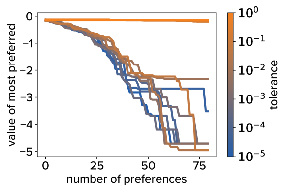
(a) Medians of the trials are plotted as a function of the number of preferences sampled.

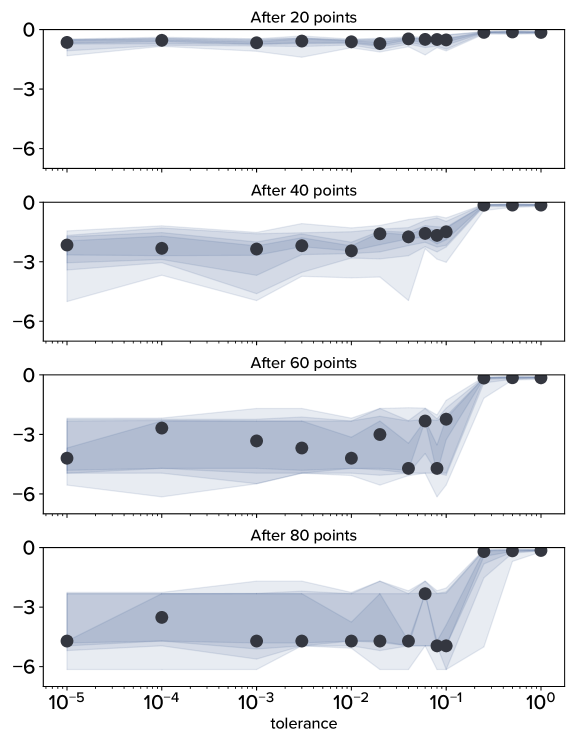
(b) Interpercentile ranges (from darkest [40-60] to lightest [10-90]) of the trials are presented as a function of tolerance. The medians are plotted with charcoal circles.

Figure 3: The convergence behavior of Algorithm 1 as tested over 20 independently trials on the Shekel05 function. While large tolerances seem to stagnate, sufficiently small values (below $~{}0.1$) move towards the minimum. Also, the lowest tolerance does not consistently perform better.

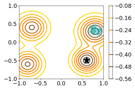
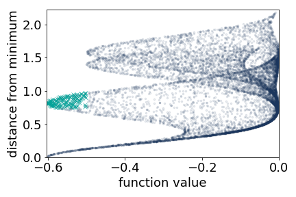
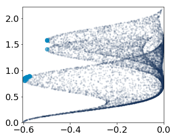
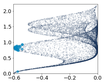
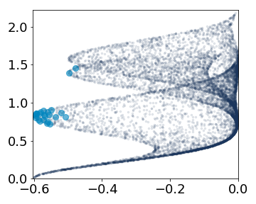
Figure 4: Results from different tolerances considered in a multi-objective setting – trying to minimize a function while being far from the true minimum. (top left): The function, with a black $\star$ for the minimum and green $\times$ for the preferred region. (top right): The feasible region showing the possible function values and their associated distance from the minimum; the green $\times$ represent the preferred region. (bottom): The final outcome found from each of 20 independent trials for tolerance 0.003 (left), 0.03 (middle) and 0.1 (right).

We now experiment to understand the impact of allowing ties into the optimization process. To do so, we phrase the preference optimization process using a scalar function $f_{\text{test}}$ and a stated tolerance $\epsilon$,

$$\begin{cases}{\mathbf{x}}^{(1)}\approx{\mathbf{x}}^{(2)},\hskip 5.69054pt\text{if},\ \ |f_{\text{test}}({\mathbf{x}}^{(1)})-f_{\text{test}}({\mathbf{x}}^{(2)})|\leq\epsilon\\ {\mathbf{x}}^{(1)}\succ{\mathbf{x}}^{(2)},\hskip 5.69054pt\text{else if},\ f_{\text{test}}({\mathbf{x}}^{(1)})<f_{\text{test}}({\mathbf{x}}^{(2)})\\ {\mathbf{x}}^{(1)}\prec{\mathbf{x}}^{(2)},\hskip 5.69054pt\text{otherwise},\end{cases}$$ (1)

In a first experiment, we consider a standard scalar test function as our $f_{\text{test}}$, the Shekel05 function McCourt (2016). We analyze the convergence behavior of Algorithm 1 on this function with a range of tolerance values between $10^{-5}$ and 1. Figure 3(a) shows the convergence behavior as dependent on tolerance.

Figure 4 shows the impact of varying tolerances on a multicriteria optimization problem using a multi-modal function in two dimensions. Success is defined as trying to reach the region containing the local minimum with the second lowest value; we approach this by balancing the competing objectives of minimizing function value and maximizing distance from the global minimum. To automate the testing process (pretend that a human was in the loop) we define a nonlinear scalarized quality function

$$f_{\text{test}}({\mathbf{x}})=[4(f({\mathbf{x}})+.6)^{3}+.3(\|{\mathbf{x}}-{\mathbf{x}}_{*}\|-2.4)^{3}]^{1/3},$$

where ${\mathbf{x}}_{*}$ is the true minimum. As we can see in the bottom portion of Figure 4, the clearest impact of tighter tolerances seems to be the narrowing down of results to be closer to the Pareto frontier.

3 Proposed Artwork Coloring Examples

The eventual goal of our preference-based optimization strategy is to be able to identify most-preferred outcomes when a scalar function such as $f_{\text{test}}$ does not exist. We now present a testing situation which lacks any such $f_{\text{test}}$: the coloring of an abstract piece of art. The shape in particular is shown in Figure 1 with two possible colorings presented, from which the user is expected to choose between them, or that they are both “roughly equal”.

The shape is a fractal, defined in Lee (2014), to have 3 polynomial roots which points in the complex domain converge to through Newton’s method at different rates. The search domain for this coloring problem is, at present, a 10 dimensional space defining 3 different colors associated with the 3 polynomial roots, transition speed between those 3 colors, and the base color (which has an effect of dulling the colors).

Our goal in running these experiments was to determine the performance of Algorithm 1 relative to a purely random search Bergstra & Bengio (2012) of the domain. In particular, users would be asked to run through some number of optimizations using random search and some number using Algorithm 1 and then a final comparison asking which would be preferred between the most-preferred from the two strategies.

3.1 Initial Testing and User Feedback

We built a webapp to provide a sequence of comparisons to users in the format of Figure 1; the incumbent most-preferred is always on the right-hand side. This was the first point of feedback that we received from users: “Why does the winner always stick around?” While it presents a viable optimization strategy, we may need to be more cognizant of the persistent presence of the ${\mathbf{x}}_{\text{best}}$ during the optimization.

Additionally, some users complained that they felt “tricked” or that we “misled” them when learning that some of the optimizations were powered by random search rather than something more intelligent/adaptive. This was surely caused by running tests on people who had already been informed of the purpose of the testing (a form of the placebo effect, perhaps). Even though testers did not know whether they were running with random search or preference optimization (to avoid a true placebo effect), some frustration around the distinction was present.

A more severe complication, and one which we had failed to consider, is the user’s sense of completion. In the pure Algorithm 1, a budget $T$ would be set at the start. It seemed, though, that users were frustrated by this fixed budget. Some commented ”Do I keep going?” or ”I think I’m done.” part way through the budget; others said ”I want to keep going.” after reaching the budget.

3.2 Proposed Next Steps

One option to address the user discomfort with always seeing ${\mathbf{x}}_{\text{best}}$ is comparisons is to consider more of a tournament strategy. While this is straightforward when randomly searching the space, it is more complicated to adapt Algorithm 1 for this situation.

To address the user’s discomfort in the process of random versus intelligent testing, we should consider not informing people how the testing process is designed and proceeding. Originally, we were afraid that testers would not find this opaque presentation reasonable, but it may be preferable to not give users any understanding as to the structure. One user commented “I wasn’t necessarily choosing what I thought was the most aesthetically pleasing but making choices to try and direct the system in a certain way that would generate better images down the road.” which is, obviously, not part of our optimization strategy.

The frustration users felt around the budget is reasonable, but not something that we immediately know how to address. One option might be to allow users to run the optimization until they “feel” it is complete; doing so changes the experimental structure but might yield additional insights into user behavior (especially regarding their tolerance).

Probably the most problematic component of this testing framework was something alluded to by users but not explicitly stated: a lack of understanding about the actual range of outcomes in the search space. Users asked ”Is this how it is supposed to look?” and ”What colors are available?” during the testing, which led us to realize that, without any sense of what could occur in the coloring, it would be difficult to confidently make judgments.

It is our hope that we can discuss these final two points with other researchers at this ICML HILL workshop and try to come away with strategies for future experimentation.

References

- Bergstra & Bengio (2012) Bergstra, J. and Bengio, Y. Random search for hyper-parameter optimization. Journal of Machine Learning Research, 13(Feb):281–305, 2012.
- Bergstra et al. (2011) Bergstra, J. S., Bardenet, R., Bengio, Y., and Kégl, B. Algorithms for hyper-parameter optimization. In Advances in Neural Information Processing Systems, pp. 2546–2554, 2011.
- Brochu et al. (2008) Brochu, E., de Freitas, N., and Ghosh, A. Active preference learning with discrete choice data. In Advances in Neural Information Processing Systems, pp. 409–416, 2008.
- Brochu et al. (2010) Brochu, E., Brochu, T., and de Freitas, N. A bayesian interactive optimization approach to procedural animation design. In Proceedings of the 2010 ACM SIGGRAPH/Eurographics Symposium on Computer Animation, pp. 103–112. Eurographics Association, 2010.
- Burger et al. (2017) Burger, R., Bharatheesha, M., van Eert, M., and Babuška, R. Automated tuning and configuration of path planning algorithms. In 2017 IEEE International Conference on Robotics and Automation (ICRA), pp. 4371–4376. IEEE, 2017.
- Cano et al. (2018) Cano, J., Yang, Y., Bodin, B., Nagarajan, V., and O’Boyle, M. Automatic parameter tuning of motion planning algorithms. In 2018 IEEE/RSJ International Conference on Intelligent Robots and Systems (IROS), pp. 8103–8109. IEEE, 2018.
- Chu & Ghahramani (2005) Chu, W. and Ghahramani, Z. Preference learning with gaussian processes. In Proceedings of the 22nd International Conference on Machine Learning, pp. 137–144. ACM, 2005.
- Dewancker et al. (2016) Dewancker, I., McCourt, M., and Ainsworth, S. Interactive preference learning of utility functions for multi-objective optimization. In NIPS Future of Interactive Learning Machines Workshop, 2016.
- Ehrgott (2005) Ehrgott, M. Multicriteria optimization, volume 491. Springer Science & Business Media, 2005.
- Frazier (2018) Frazier, P. I. Bayesian optimization. In Recent Advances in Optimization and Modeling of Contemporary Problems, pp. 255–278. INFORMS, 2018.
- Gonzalez et al. (2017) Gonzalez, J., Dai, Z., Damianou, A., and Lawrence, N. D. Preferential bayesian optimization. arXiv preprint arXiv:1704.03651, 2017.
- Guo et al. (2010) Guo, S., Sanner, S., and Bonilla, E. V. Gaussian process preference elicitation. In Advances in Neural Information Processing Systems, pp. 262–270, 2010.
- Houlsby et al. (2012) Houlsby, N., Huszar, F., Ghahramani, Z., and Hernández-Lobato, J. M. Collaborative gaussian processes for preference learning. In Advances in Neural Information Processing Systems, pp. 2096–2104, 2012.
- Hutter et al. (2011) Hutter, F., Hoos, H. H., and Leyton-Brown, K. Sequential model-based optimization for general algorithm configuration. In Learning and Intelligent Optimization, pp. 507–523. Springer, 2011.
- Knowles (2006) Knowles, J. ParEGO: a hybrid algorithm with on-line landscape approximation for expensive multiobjective optimization problems. IEEE Transactions on Evolutionary Computation, 10(1):50–66, 2006.
- Lee (2014) Lee, E. H. Alternating newton’s method. github.com/ericlee0803/NewtonEllipsoid, 2014.
- McCourt (2016) McCourt, M. Optimization Test Functions. github.com/sigopt/evalset, 2016.
- Pinsler et al. (2018) Pinsler, R., Akrour, R., Osa, T., Peters, J., and Neumann, G. Sample and feedback efficient hierarchical reinforcement learning from human preferences. In 2018 IEEE International Conference on Robotics and Automation (ICRA), pp. 596–601. IEEE, 2018.
- Ranganath et al. (2013) Ranganath, R., Gerrish, S., and Blei, D. M. Black box variational inference. arXiv preprint arXiv:1401.0118, 2013.
- Rao & Kupper (1967) Rao, P. and Kupper, L. L. Ties in paired-comparison experiments: A generalization of the bradley-terry model. Journal of the American Statistical Association, 62(317):194–204, 1967.
- Shahriari et al. (2016) Shahriari, B., Swersky, K., Wang, Z., Adams, R. P., and De Freitas, N. Taking the human out of the loop: A review of bayesian optimization. Proceedings of the IEEE, 104(1):148–175, 2016.
- Snoek et al. (2012) Snoek, J., Larochelle, H., and Adams, R. P. Practical bayesian optimization of machine learning algorithms. In Advances in Neural Information Processing Systems, pp. 2951–2959, 2012.
- Thatte et al. (2017) Thatte, N., Duan, H., and Geyer, H. A sample-efficient black-box optimizer to train policies for human-in-the-loop systems with user preferences. IEEE Robotics and Automation Letters, 2(2):993–1000, 2017.
- Tran et al. (2016) Tran, D., Kucukelbir, A., Dieng, A. B., Rudolph, M., Liang, D., and Blei, D. M. Edward: A library for probabilistic modeling, inference, and criticism. arXiv preprint arXiv:1610.09787, 2016.
- Wirth et al. (2017) Wirth, C., Akrour, R., Neumann, G., and Fürnkranz, J. A survey of preference-based reinforcement learning methods. The Journal of Machine Learning Research, 18(1):4945–4990, 2017.