Rotating Equilibria of Vortex Sheets

Abstract

We consider relative equilibrium solutions of the two-dimensional Euler equations in which the vorticity is concentrated on a union of finite-length vortex sheets. Using methods of complex analysis, more specifically the theory of the Riemann-Hilbert problem, a general approach is proposed to find such equilibria which consists of two steps: first, one finds a geometric configuration of vortex sheets ensuring that the corresponding circulation density is real-valued and also vanishes at all sheet endpoints such that the induced velocity field is well-defined; then, the circulation density is determined by evaluating a certain integral formula. As an illustration of this approach, we construct a family of rotating equilibria involving different numbers of straight vortex sheets rotating about a common center of rotation and with endpoints at the vertices of a regular polygon. This equilibrium generalizes the well-known solution involving single rotating vortex sheet. With the geometry of the configuration specified analytically, the corresponding circulation densities are obtained in terms of a integral expression which in some cases lends itself to an explicit evaluation. It is argued that as the number of sheets in the equilibrium configuration increases to infinity, the equilibrium converges in a certain distributional sense to a hollow vortex bounded by a constant-intensity vortex sheet, which is also a known equilibrium solution of the two-dimensional Euler equations.

1 Introduction

Relative equilibria represent a particularly important class of solutions of equations governing the motion of fluids. This is because if they are stable then such equilibria describe flow structures which can persist for long times. Here we are interested in two-dimensional (2D) flows of inviscid incompressible fluids with localized vorticity, although models similar to the ones developed here are also relevant for plasmas and quantum fluids, in particular, Bose-Einstein condensates. Arguably, the best-known equilibrium solutions characterizing such flows involve point vortices where the vorticity is supported as Dirac measures on a set of discrete points. There exists a very rich literature on this topic and we refer the reader to the review papers [3, 4, 9, 19] for a survey. Desingularization of point vortices by replacing them with finite-area regions of constant vorticity leads to the so-called vortex-patch problem which is of the free-boundary type, since the shapes of the patch boundaries need to be found as a part of the solution of the problem. Such problems have also received significant attention starting with the seminal work of Pierrehumbert [25], Saffman & Szeto [29], Dritschel [10], Kamm [14], Moore et al. [17], and in this context we also mention a more recent investigation [15]. Some theoretical results concerning the desingularization process can be found in [32] and [11].

Vortex sheets represent discontinuities of the tangential velocity component, such that vorticity is localized along one-dimensional (1D) curves [28]. They have received attention especially in the context of fluid-structure interaction where they have been used as simple models of vortex shedding [13, 12, 30, 2]. However, unlike the case of point-vortex or vortex-patch equilibria, our knowledge of equilibrium configurations involving vortex sheets is rather limited. Two closed-form solutions are available as regards equilibria involving closed or unbounded vortex sheet (i.e., sheets possessing no endpoints): the circular vortex sheet and the infinite (or periodic) straight vortex sheet, both with constant circulation density and defined in an unbounded domain [7, 28]. Closed vortex sheets play a role in the Sadovskii flows [27] in which they separate regions with constant vorticity from the irrotational flow and they were also used to construct “hollow vortices” in which the vortex sheet separates a stagnant region of the flow from the region in potential motion [26, 5]. More recently such configurations were obtained for flows past an obstacle [31]. A distinguishing feature of all of these solutions is that closed vortex sheets separate regions characterized by different values of the Bernoulli constant.

As regards relative equilibria involving non-closed vortex sheets, i.e., flows in which the vorticity support is not a closed curve, there is one solution known in the analytic form, namely, a straight sheet of length $2a$ ($a>0$) rotating about its center with the angular velocity $\omega$ [7]. The circulation density is given by

$$\gamma(x)=\omega\sqrt{a^{2}-x^{2}},\qquad x\in[-a,a],$$ (1)

and, as shown in [7], this equilibrium can be regarded as the limiting solution obtained from Kirchhoff’s rotating ellipse by fixing its major axis and letting the minor axis vanish while allowing the vorticity to become unbounded in such a way that the circulation remains constant. Several approximations of relative sheet equilibria were computed by O’Neil [21], see also [22], who represented the sheets using a number of unconnected point vortices arranged along finite arcs. More recently, an exact method has been devised by the same author to compute relative equilibrium configurations involving both vortex sheets and point vortices [24, 23].

In the present investigation we introduce a novel approach allowing one to construct a family of rotating equilibria involving vortex sheets which generalizes the equilibrium solution (1). Hereafter heavy use will be made of complex notation. Assuming that $z(\xi,t)=x(\xi,t)+iy(\xi,t)$ represents the position at time $t$ of a point on a vortex sheet $L$ corresponding to the arc-length parameter $\xi$, the evolution of the sheet is governed by the Birkhoff-Rott singular integro-differential equation [28]

$${\frac{\partial z^{\ast}}{\partial t}}(\xi,t)=V(z(\xi,t))\,\equiv\,\frac{1}{\pi i}\mbox{pv}\int_{L}\frac{\gamma(s)}{z(s,t)-z(\xi,t)}\,ds,$$ (2)

where $\gamma(s)$ is the circulation density of the vortex sheet which can be interpreted as the difference between the tangential velocity components on the two sides of the sheet and the asterisk denotes complex conjugation. In (2) integration is defined in the sense of Cauchy’s principal value. We note that in general the sheet $L$ may consist of a number of disjoint segments. Because of its ill-posed nature, the Birkhoff-Rott equation (2) has generated a lot of interest in the applied mathematics literature [8, 16]. Since we are interested here in relative equilibria, i.e., equilibria attained in a moving — rotating or translating — frame of reference, the complex velocity $V(z)=(u-iv)(z)$, where $u$ and $v$ are, respectively, the $x$ and $y$ components, will be given in terms of some prescribed function $f(z)$ independent of time. For relative equilibria rotating with the rate of rotation $\omega\in{\mathbb{R}}$, this function has the form $f(z)=i\omega z^{*}$, whereas for relative equilibria translating with a constant velocity $U\in{\mathbb{C}}$, it has the form $f(z)=U$. We note that in either case the function $f(z)$ is defined up to an arbitrary real multiplicative constant which can be factored out by rescaling the circulation density $\gamma(s)$.

The particular question we consider in this study is whether there exist relative equilibrium solutions of the Birkhoff-Rott equation (2) consisting of a certain number $p\geq 1$ of sheets $L_{m}$, $m=0,\dots,p-1$, assumed disjoint, possibly except for a finite number of points of contact, such that we have $L=\bigcup_{m=0}^{p-1}L_{m}$ in (2). The endpoints of the sheets will be denoted $a_{m},b_{m}\in{\mathbb{C}}$ ($a_{m},b_{m}\in L_{m}$), $m=0,\dots,p-1$. Thus, the problem of finding such relative equilibria is equivalent to the question whether the integral equation

$$\frac{1}{\pi i}\mbox{pv}\int_{L}\frac{\gamma(s)\,ds}{z(s)-z(\xi)}=f(z),\qquad\forall z(\xi)\in L$$ (3)

admits suitable solutions. We emphasize that by “solution” we mean here the pair $\{L,\gamma\}$ representing the geometry of the vortex sheet and the corresponding real-valued distribution of the circulation density.

Using methods of complex analysis, more specifically, the Riemann-Hilbert theory, we develop a constructive approach allowing one to obtain relative equilibrium solutions to (3) which in some situations are given in a closed form. In this formulation the problems of determining the shapes $L$ of the sheets and the corresponding circulation densities $\gamma$ decouple: first, one needs to find the sheets $L$ satisfying certain conditions after which obtaining the circulation density $\gamma$ reduces to evaluating an integral formula. In this sense, there is an analogy between the proposed approach and the “Brownian ratchet” method developed by Newton to find relative equilibria of point vortices [20, 6]. Using the proposed approach we then construct a family of rotating equilibrium configurations consisting of a different number of sheets each with one endpoint at the center of rotation and the other at a vertex of a polygon. This family generalizes the well-known equilibrium solution (1) describing a single rotating sheet and in a certain “weak” sense approaches a hollow vortex bounded by a closed constant-density vortex sheet when the number of sheets $p$ increases to infinity.

The structure of the paper is as follows: in the next section we describe the connection between the questions considered here and the Riemann-Hilbert problem in complex analysis which allows us to formulate our approach; then in Section 3 we introduce a particular family of configurations of rotating vortex sheets, prove that they constitute relative equilibria and and obtain expressions for the circulation densities; next, in Section 4, we describe and validate a numerical approach needed to evaluate these formulas; the results are presented in Section 5, whereas discussion and final conclusions are deferred to Section 6.

2 Vortex Sheets and the Riemann-Hilbert Problem

In this section we first elucidate the relation between the problem considered here and the Riemann-Hilbert problem of complex analysis. Then, some elements of the theory of this problem will be used to formulate a two-step solution approach. Given a contour on the complex plane, the Riemann-Hilbert problem consists in finding a holomorphic function defined in the complement of this contour on the complex plane such that its limiting values on both sides of the contour satisfy a prescribed relation [1]. Since holomorphic functions are conveniently expressed in terms of singular (Cauchy-type) integrals, there is a natural connection between the Riemann-Hilbert problem and the theory of singular integral equations.

In a similar spirit, to determine a relative equilibrium involving vortex sheets we need to find a velocity field, which for potential (i.e., incompressible and irrotational) flows is represented in terms of a holomorphic function $V(z)$, $z\in{\mathbb{C}}\backslash L$, satisfying the following kinematic conditions on the contour (sheet) $L$

$$V^{+}(t)-V^{-}(t)=\gamma(t)\frac{dt}{ds}(t),\qquad t\in L,$$ (4)

where $t=t(s)$ represents the parameterization of the contour $L$ in terms of its arc length $s$, whereas $V^{\pm}(t)$ are the limits of the velocity field $V(z)$ as $z\rightarrow t\in L$ on the two sides of the contour. Condition (4) implies that the normal velocity component on both sides of the sheet is the same and the tangential velocity component has a jump equal to the prescribed circulation density $\gamma$ (the continuity of pressure across the sheet then follows from these conditions and the Bernoulli equation). For the Riemann-Hilbert problem to be completely defined [1], relation (4) must be complemented by a condition specifying the behavior of the function $V(z)$ as $|z|\rightarrow\infty$, which is determined by the function $f(z)$. These conditions together are equivalent to relation (3) and thus the question of the existence of relative equilibria involving vortex sheets can be recast in terms of whether equation (3) admits suitable solutions.

Aspects of the Riemann-Hilbert problem relevant to the questions considered here are reviewed in monograph [18], from which we have adopted parts of the notation. First, the integral expressing velocity needs to be recast as a complex integral defined with respect to the complex variable $t$, i.e., for any $\zeta\in{\mathbb{C}}\,\backslash\,L$ we have

$$V(\zeta)=\frac{1}{2\pi i}\int_{L}\frac{\gamma(t(s))\,ds}{t(s)-\zeta}=\frac{1}{2\pi i}\int_{L}\frac{\varphi(t)\,dt}{t-\zeta},$$ (5)

where the density is defined as

$$\quad\varphi(t):=\gamma(t)\left(\frac{dt}{ds}\right)^{-1}.$$ (6)

Problem (3) can then be recast in a canonical form consistent with the Riemann-Hilbert problem, namely

$$\frac{1}{\pi i}\mbox{pv}\int_{L}\frac{\varphi(t)\,dt}{t-z}=f(z),\qquad\forall\in L.$$ (7)

Then, we note that in order for the velocity (5) to be bounded everywhere in ${\mathbb{C}}\,\backslash\,L$, the density $\varphi(t)$, cf. (6), must satisfy certain conditions, namely, it must be Hölder-continuous with some Hölder index $0<\mu\leq 1$ and must vanish at all sheet endpoints [18], i.e.,

$$\varphi(a_{m})=\varphi(b_{m})=0,\quad m=0,\dots,p-1.$$ (8)

This last condition in particular will play an essential role in our analysis below.

In general, problem (7) admits solutions $\varphi$ which vanish at $p$ endpoints only [18]. In order for the densities $\varphi$ obtained from (7) to vanish at all $2p$ endpoints (which is necessary for the corresponding velocity field (5) to be well-defined everywhere), the sheets $L$ and the function $f(z)$ in (7) must satisfy the following set of compatibility condition [18, relation (89.14)] (in essence, there is one condition for each additional endpoint on which $\varphi(t)$ is to vanish)

$$C_{n}:=\int_{L}\frac{t^{n}f(t)\,dt}{\sqrt{R_{p}(t)}}=0,\quad n=0,\dots,p-1,$$ (9)

where

$$R_{p}(z):=\prod_{m=1}^{p}(z-a_{m})(z-b_{m}),$$ (10)

where “$:=$” means “equal to by definition”. Since the function $f(z)$ is fixed and determined by the type of the relative equilibrium sought (rotating or translating), conditions (9) can be interpreted as constraints on the shapes of the vortex sheet $L$ which must be satisfied in order for the corresponding velocity field (5) to be well defined. In addition, it must also be ensured that the resulting circulation density is real-valued which can often be done based on some symmetry arguments (cf. Section 3 below). Then, a density satisfying conditions (8) is given by the following formula [18, relation (88.9)]

$$\varphi(z)=\frac{\sqrt{R_{p}(z)}}{\pi i}\int_{L}\frac{f(t)\,dt}{\sqrt{R_{p}(t)}(t-z)}=0,\quad z\in L.$$ (11)

Finally, the real-valued circulation density $\gamma$ needed for the Birkhoff-Rott equation (3) can be obtained from (11) and (6) using the known parameterization of the contour.

The above facts demonstrate how the problems of finding the equilibrium shapes of vortex sheets and the corresponding circulation densities are related to each other. They also suggest the following general and constructive approach to finding relative equilibria involving vortex sheets

1. find arcs $L_{0},\dots,L_{p-1}$ such that the compatibility conditions (9) are satisfied and the imaginary part of $\varphi(t)\frac{dt}{ds}(t)$ vanishes,

2. determine the corresponding circulation densities by evaluating formula (11) and using (6).

In the next section we implement this procedure in order to find a new family of equilibrium solutions consisting of an arbitrarily large number of rotating vortex sheets which generalizes the well-known solution (1).

3 Rotating Equilibria

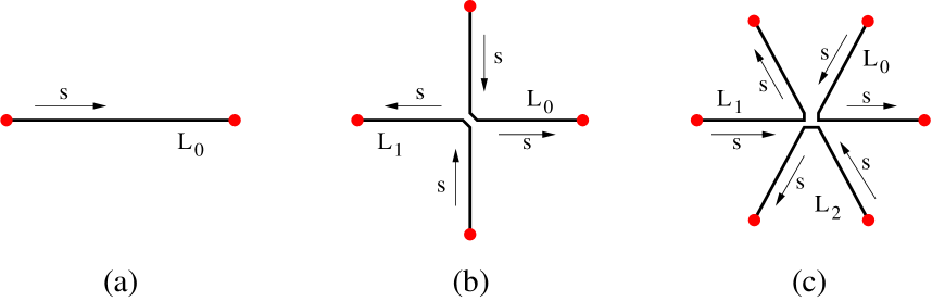
Figure 1: Schematic representation of the arrangement of (a) $p=1$, (b) $p=2$ and (c) $p=3$ bent sheets into a polygonal configuration. Red circles mark the endpoints on which conditions (8) apply, whereas arrows represent the parameterization used in (13). When $p\geq 2$ midpoints of the sheets come into contact at the center of rotation.

In this section we first consider a particular arrangement of vortex sheets and demonstrate, through a rigorous proof, that it can form a rotating equilibrium, cf. Step 1 in Section 2. Then, as Step 2, we obtain a closed-form integral formula for the circulation density of the sheet which in the simplest cases lends itself to explicit evaluation. Since we focus on rotating equilibria, we now set $f(z)=i\omega z^{*}$ and consider an arrangement of $p$ bent sheets with common midpoints, cf. figure 1 (the choice of this particular configuration as a candidate for a relative equilibrium was inspired by our earlier computational experiments). As will be shown below, due to their symmetry properties these configurations always produce purely-real circulation densities. In order to parameterize this configuration, we first define the $2p$th complex root of unity as

$$\sigma=\exp\left(\frac{2\pi i}{2p}\right)$$ (12)

with the properties that $\sigma^{2p}=1$ and $|\sigma|=1$. We note that $\sigma^{m}$, $m=0,\dots,2p-1$ are the complex coordinates of the vertices of a regular $2p$-gon inscribed in a unit circle. The sheets are then described as, cf. figure 1,

$$L_{m}\ :\ z_{m}(s)=\left\{\begin{array}[]{rr}-\sigma^{2m+1}s,&-1\leqq s\leqq 0,\\ \sigma^{2m}s,&0\leqq s\leqq 1,\end{array}\right.$$ (13)

for $m=0,1,\dots,p-1$ with

$$z^{\prime}_{m}(s)=\left\{\begin{array}[]{rr}-\sigma^{2m+1},&-1\leqq s\leqq 0,\\ \sigma^{2m},&0\leqq s\leqq 1.\end{array}\right.,$$

where the prime denotes differentiation with respect to the arc length parameter $s\in[-1,1]$. The endpoints of the $m$th sheet $L_{m}$ then are $a_{m}=z_{m}(-1)=\sigma^{2m+1}$ and $b_{m}=z_{m}(1)=\sigma^{2m}$, such that the function $R_{p}(z)$, cf. (10), can be expressed as

$$R_{p}(z)=\prod_{m=0}^{p-1}(z-\sigma^{2m})(z-\sigma^{2m+1})=\prod_{m=0}^{2p-1}(z-\sigma^{m}).$$ (14)

We observe that the function $R_{p}(z)$ is invariant under multiplication of its argument by $\sigma^{\ell}$ for any $\ell\in{\mathbb{N}}$

$$R_{p}(\sigma^{\ell}z)=\prod_{m=0}^{2p-1}(\sigma^{\ell}z-\sigma^{m})=\sigma^{2p\ell}\prod_{m=0}^{2p-1}(z-\sigma^{m-\ell})=\prod_{m=0}^{2p-1}(z-\sigma^{m-\ell})=R_{p}(z)$$ (15)

because this operation is equivalent to rotating the $2p$-gon formed by the sheet endpoints by the angle $\ell\pi/p$, a transformation which leaves this polygon invariant.

We are now in the position to state the following proposition

Proposition 1.

Assuming the vortex sheets $L_{m}$, $m=0,\dots,p-1$ are defined by expression (13) and that $f(z)=i\omega z^{*}$, the compatibility conditions (9) are satisfied for any positive integer $p$.

Proof.

We begin by observing that, because of property (15), the denominators in the integrand expressions in constraints (9) remain unchanged when the constraint expressions are evaluated for different sheets. Thus, noting that

$$C_{n}=i\omega\int_{L}\frac{t^{n}t^{*}\,dt}{\sqrt{R_{p}(t)}}=i\omega\sum_{m=0}^{p-1}\int_{L_{m}}\frac{t^{n}t^{*}\,dt}{\sqrt{R_{p}(t)}},\quad n=0,\dots,p-1,$$

we obtain for the integral defined on the $m$th sheet when $n=0$

$$i\omega\int_{L_{m}}\frac{t^{*}}{\sqrt{R_{p}(t)}}\,dt =i\omega\int_{-1}^{0}\frac{(-\sigma^{\ast})^{2m+1}s}{\sqrt{R_{p}(t(s))}}(-\sigma)^{2m+1}\,ds+i\omega\int_{0}^{1}\frac{(\sigma^{\ast})^{2m}s}{\sqrt{R_{p}(t(s))}}\sigma^{2m}\,ds$$

$$=i\omega\int_{-1}^{0}\frac{s}{\sqrt{R_{p}(t(s))}}\,ds+i\omega\int_{0}^{1}\frac{s}{\sqrt{R_{p}(t(s))}}\,ds=0,\quad m=0,\dots,p-1,$$ (16)

which is true because the expression in the denominator, cf. (10), remains the same for all sheets $L_{m}$, cf. (15). Hence, we have $C_{0}=0$. Then, when $1\leqq n<p$, owing to the identity $z^{k}z^{*}dz=z^{k-1}|z|^{2}dz$, the integral corresponding to the $m$th sheet becomes, again recognizing property (15),

$$i\omega\int_{L_{m}}\frac{t^{n}t^{*}}{\sqrt{R_{p}(t)}}\,dt =i\omega\int_{-1}^{0}\frac{(-\sigma^{2m+1})^{n-1}s^{n+1}}{\sqrt{R_{p}(t(s))}}(-\sigma^{2m+1})\,ds+i\omega\int_{0}^{1}\frac{(\sigma^{2m})^{n-1}s^{n+1}}{\sqrt{R_{p}(t(s))}}\sigma^{2m}\,ds$$

$$=i\omega\int_{-1}^{0}\frac{(-1)^{n}\sigma^{(2m+1)n}s^{n+1}}{\sqrt{R_{p}(t(s))}}\,ds+i\omega\int_{0}^{1}\frac{\sigma^{2mn}s^{n+1}}{\sqrt{R_{p}(t(s))}}\,ds.$$

Adding up the integrals corresponding to the sheets $L_{m}$, $m=0,\dots,p-1$, we obtain

$$C_{n} =i\omega(-1)^{n}\sum_{m=0}^{p-1}\sigma^{(2m+1)n}\int_{-1}^{0}\frac{s^{n+1}}{\sqrt{R_{p}(t(s))}}\,ds+i\omega\sum_{m=0}^{p-1}\sigma^{2mn}\int_{0}^{1}\frac{s^{n+1}}{\sqrt{R_{p}(t(s))}}\,ds$$

$$=i\omega\left[-\sum_{m=0}^{p-1}\sigma^{(2m+1)n}+\sum_{m=0}^{p-1}\sigma^{2mn}\right]\int_{0}^{1}\frac{s^{n+1}\,ds}{\sqrt{R_{p}(t(s))}}$$

$$=i\omega\left[\sum_{m=0}^{p-1}\sigma^{2mn}\right]\left(1-\sigma^{n}\right)\int_{0}^{1}\frac{s^{n+1}\,ds}{\sqrt{R_{p}(t(s))}}=0,\quad n=1,\dots,p-1,$$ (17)

which vanishes because due to the properties of the geometric progression and the fact that $\sigma^{2n}\neq 1$ for $n=1,\dots,p-1$ we have

$$\sum_{m=0}^{p-1}\sigma^{2mn}=\frac{1-\sigma^{2pn}}{1-\sigma^{2n}}=0.$$

Thus, relations (16) and (17) prove our claim. ∎

Having established that the configuration of $p$ bent vortex sheets defined in (13), cf. figure 1, can give rise to a rotating equilibrium, we now proceed to determine the density $\varphi_{p}(z)$ using formula (11) which we transform as follows in order to reduce it to a definite integral on $[0,1]$

$$\varphi_{p}(z) =\frac{\sqrt{R_{p}(z)}}{\pi i}\int_{L}\frac{i\omega t^{*}\,dt}{\sqrt{R_{p}(t)}(t-z)}=\frac{\omega}{\pi}\sqrt{R_{p}(z)}\int_{L}\frac{t^{*}\,dt}{\sqrt{R_{p}(t)}(t-z)}$$

$$=\frac{\omega}{\pi}\sqrt{R_{p}(z)}\sum_{m=0}^{p-1}\int_{L_{m}}\frac{t^{*}\,dt}{\sqrt{R_{p}(t)}(t-z)}$$

$$=\frac{\omega}{\pi}\sqrt{R_{p}(z)}\sum_{m=0}^{p-1}\left[\int_{-1}^{0}\frac{(-\sigma^{2m+1})^{*}s(-\sigma^{2m+1})\,ds}{\sqrt{R_{p}(-\sigma^{2m+1}s)}(-\sigma^{2m+1}s-z)}+\int_{0}^{1}\frac{(\sigma^{2m})^{*}s(\sigma^{2m})\,ds}{\sqrt{R_{p}(\sigma^{2m}s)}(\sigma^{2m}s-z)}\right]$$

$$=\frac{\omega}{\pi}\sqrt{R_{p}(z)}\sum_{m=0}^{p-1}\left[\int_{-1}^{0}\frac{-s\,ds}{\sqrt{R_{p}(s)}(\sigma^{2m+1}s+z)}+\int_{0}^{1}\frac{s\,ds}{\sqrt{R_{p}(s)}(\sigma^{2m}s-z)}\right]$$ (18)

$$=\frac{\omega}{\pi}\sqrt{R_{p}(z)}\sum_{m=0}^{p-1}\int_{0}^{1}\left[\frac{-s}{\sqrt{R_{p}(s)}(\sigma^{2m+1}s-z)}+\frac{s}{\sqrt{R_{p}(s)}(\sigma^{2m}s-z)}\right]\,ds$$

$$=\frac{\omega}{\pi}\sqrt{R_{p}(z)}\int_{0}^{1}\frac{s}{\sqrt{R_{p}(s)}}\sum_{m=0}^{p-1}\left(\frac{-1}{\sigma^{2m+1}s-z}+\frac{1}{\sigma^{2m}s-z}\right)\,ds.$$ (19)

Before obtaining a simple formula for the circulation density valid for any $p\geq 1$, we first derive its particular instances for $p=1,2,3$. When $p=1$, cf. figure 1(a), we have $\sigma=\exp(i\pi)=-1$ and $R_{1}(z)=(z-1)(z+1)=z^{2}-1$. Then, from (18) we deduce

$$\varphi_{1}(z) =\frac{\omega}{\pi}\sqrt{R_{1}(z)}\left[\int_{-1}^{0}\frac{-s\,ds}{\sqrt{R_{1}(s)}(-s+z)}+\int_{0}^{1}\frac{s\,ds}{\sqrt{R_{1}(s)}(s-z)}\right]$$

$$=\frac{\omega}{\pi}\sqrt{R_{1}(z)}\int_{-1}^{1}\frac{s\,ds}{\sqrt{R_{1}(s)}(s-z)}.$$ (20)

At the same time, formula (19) also gives rise to

$$\varphi_{1}(z)=\frac{\omega}{\pi}\sqrt{R_{1}(z)}\int_{0}^{1}\frac{s}{\sqrt{R_{1}(s)}}\left(\frac{-1}{-s-z}+\frac{1}{s-z}\right)\,ds=\frac{\omega}{\pi}\sqrt{R_{1}(z)}\int_{0}^{1}\frac{2s^{2}\,ds}{\sqrt{R_{1}(s)}(s^{2}-z^{2})}$$ (21)

which is equivalent to (20).

Next, for $p=2$, cf. figure 1(b), substituting $\sigma=\exp(i\pi/2)=i$, $\sigma^{2}=-1$, $\sigma^{3}=-\sigma=-i$ and $R_{p}(z)=R_{2}(z)=z^{4}-1$ into (19), we obtain

$$\varphi_{2}(z) =\frac{\omega}{\pi}\sqrt{R_{2}(z)}\int_{0}^{1}\frac{s}{\sqrt{R_{2}(s)}}\left(\frac{-1}{\sigma s-z}+\frac{1}{s-z}+\frac{-1}{-\sigma s-z}+\frac{1}{-s-z}\right)\,ds$$

$$=\frac{\omega}{\pi}\sqrt{R_{2}(z)}\int_{0}^{1}\frac{s}{\sqrt{R_{2}(s)}}\left(\frac{2z}{s^{2}+z^{2}}+\frac{2z}{s^{2}-z^{2}}\right)\,ds$$

$$=\frac{\omega}{\pi}\sqrt{R_{2}(z)}\int_{0}^{1}\frac{4zs^{3}}{\sqrt{R_{2}(s)}(s^{4}-z^{4})}\,ds.$$ (22)

Then, for $p=3$, cf. figure 1(c), using $\sigma=\exp(i\pi/3)$ we obtain the relations $\sigma^{3}=-1$, $\sigma^{4}=-\sigma=(\sigma^{2})^{\ast}=\sigma^{-2}$ and $\sigma^{5}=\sigma^{\ast}=-\sigma^{2}=\sigma^{-1}$, such that we have

$$R_{3}(z)=(z-1)(z-\sigma)(z-\sigma^{2})(z-\sigma^{3})(z-\sigma^{4})(z-\sigma^{5})=z^{6}-1.$$ (23)

Rewriting (19) as $\varphi_{p}(z)=\frac{\omega}{\pi}\sqrt{R_{p}(z)}\int_{0}^{1}\frac{s}{\sqrt{R_{p}(s)}}F_{p}(s,z)\,ds$ we obtain the following expression for the factor $F_{p}(s,z)$ when $p=3$

$$F_{3}(s,z) =\sum_{m=0}^{2}\left(\frac{-1}{\sigma^{2m+1}s-z}+\frac{1}{\sigma^{2m}s-z}\right)$$

$$=2s\left[\frac{1}{s^{2}-z^{2}}-\frac{s^{2}-z^{2}}{s^{4}+z^{2}s^{2}+z^{4}}\right]=\frac{6z^{2}s^{3}}{s^{6}-z^{6}},$$ (24)

so that in this case relation (19) becomes

$$\varphi_{3}(z)=\frac{\omega}{\pi}\sqrt{R_{3}(z)}\int_{0}^{1}\frac{6z^{2}s^{4}}{\sqrt{R_{3}(s)}(s^{6}-z^{6})}\,ds.$$ (25)

In order to extrapolate these calculations to an arbitrary number $p$ of sheets we use the following lemma

Lemma 1.

For $0<p\in{\mathbb{Z}}$, $0\neq s\in{\mathbb{R}}$ and $\sigma=\mbox{e}^{i\frac{\pi}{p}}$, the following equality holds.

$$\sum_{k=0}^{2p-1}\frac{(-1)^{k}}{z-\sigma^{k}s}=\frac{2ps^{p}z^{p-1}}{z^{2p}-s^{2p}},\quad z\in\mathbb{C}.$$ (26)

Proof.

The function

$$G(z)=\frac{2ps^{p}z^{p-1}}{z^{2p}-s^{2p}}$$

has poles at $z=\sigma^{k}s$, $k=0,\dots,2p-1$, and the residues $\alpha_{k}$ around these poles are given by

$$\alpha_{k}=\lim_{z\rightarrow\sigma^{k}s}(z-\sigma^{k}s)G(z)=\mbox{e}^{-i\pi k}=(-1)^{k},\quad k=0,\dots,2p-1.$$

Since the function

$$G(z)-\sum_{k=0}^{2p-1}\frac{(-1)^{k}}{z-\sigma^{k}s},\quad z\in{\mathbb{C}}$$

is entire on the whole complex plane, it must be constant owing to Liouville’s theorem. Moreover, since this function vanishes as $z\rightarrow\infty$, this constant is zero, which completes the proof. ∎

Using relation (26) in (19), we then obtain

$$\varphi_{p}(z)=\frac{\omega}{\pi}\sqrt{1-z^{2p}}\int_{0}^{1}\frac{2pz^{p-1}s^{p+1}}{\sqrt{1-s^{2p}}(s^{2p}-z^{2p})}\,ds,\quad z\in[0,1].$$ (27)

We remark that since the integrand expression in (27) is purely real and the integral is over the segment $[0,1]$ of the real axis, the quantity defined by (27) is purely real. The circulation density $\gamma(s)$ appearing in the Birkhoff-Rott equation (3) can then be deduced from (27) using relation (6) and will also be purely real, as needed. Noting that since on the contour $[0,1]$ we have $t=s$, we can conclude that $\gamma_{p}(s)=\varphi_{p}(s)$, i.e., expression (27) can be interpreted as the circulation densities for different values of $p$. Consequently, we obtain the following main theorem.

Theorem 1.

The configuration of $p$ bent vortex sheets (13) with the circulation density (27) is a relative equilibrium rotating with a constant rate of rotation $\omega$ around the origin.

Since the rate of rotation $\omega$ is arbitrary, without loss of generality hereafter we set $\omega=1$. The integral formula (27) can in some cases be evaluated explicitly. For example, using the symbolic software Maple, we obtain the following explicit expressions for $\gamma_{1}(s)$ and $\gamma_{2}(s)$, $s\in[0,1]$,

$$\gamma_{1}(s) =\sqrt{1-s^{2}},$$ (28a)

$$\gamma_{2}(s) =2s\operatorname{arcCoth}\left(\frac{1}{\sqrt{1-s^{4}}}\right),$$ (28b)

where we note that (28a) is equivalent to the well-known formula (1) with $\omega=1$ and $a=1$. On the other hand, formula (28b) appears to be a new solution. Evaluation of formula (27) for $p\geqq 3$ requires numerical approximation and our approach is described in the next section.

4 Numerical Approach

The integral in formula (27) involves singularities at $s=z$ and at $s=1$, hence its numerical evaluation requires special care and in this section we first introduce our numerical approach which is then validated against the exact expression (28b) corresponding to the case $p=2$. While integral formula (27) is elegant due to its compactness, it does not directly lend itself to an accurate approximation with a quadrature. We thus proceed by isolating the terms representing the singularity at $s=z$, so that the corresponding Cauchy-type integrals can be evaluated explicitly. The integrals involving the remaining terms are then approximated with a standard quadrature after the singularity at $s=1$ is eliminated with a suitable change of variables.

For convenience, when evaluating the singular part we will simultaneously consider contributions from the contours $[-1,0]$ and $[0,1]$ (both of which are present in the equilibrium configuration $L$ for all values of $p$, cf. figure 1). Defining $I_{p}:=\int_{0}^{1}\frac{2pz^{p-1}s^{p+1}}{\sqrt{-R(s)}(s^{2p}-z^{2p})}\,ds$, such that $\varphi_{p}(z)=\frac{\omega}{\pi}\sqrt{-R_{p}(z)}\,I_{p}(z)$ in (27), and

$$G_{p}(s,z)=\sum_{\begin{subarray}{c}m=1\\ m\neq p\end{subarray}}^{2p-1}\frac{(-1)^{m}}{\sigma^{m}s-z},$$ (29)

we obtain $I_{p}(z)=I^{s}_{p}(z)+I^{r}_{p}(z)$, where the singular and regular parts, respectively, $I^{s}_{p}(z)$ and $I^{r}_{p}(z)$, are represented as follows for $p=1,2,\dots$

$$I_{p}^{s}(z)=\left\{\begin{aligned} &\int_{0}^{1}\frac{2zs\,ds}{\sqrt{-R_{p}(s)}(s^{2}-z^{2})},&\qquad&p\ \text{even}\\ &\int_{0}^{1}\frac{2s^{2}\,ds}{\sqrt{-R_{p}(s)}(s^{2}-z^{2})},&\qquad&p\ \text{odd}\end{aligned}\right.,$$ (30)

and

$$I_{p}^{r}(z)=\int_{0}^{1}\frac{s}{\sqrt{-R_{p}(s)}}G_{p}(s,z)\,ds.$$ (31)

We remark here that $R_{p}(z)=z^{2p}-1\leq 0$ for any $z\in[0,1]$. Hence, the “-” sign preceding $R_{p}(z)$ ensures that the square root is real-valued.

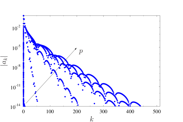
Figure 2: Dependence of the magnitude of the Fourier coefficients $a_{k}$ of the function $f_{p}(\theta)$, cf. (33), on the wavenumber $k$ for different values of $p=10,109,208,\dots,1000$. The trend with the increase of $p$ is indicated by an arrow.

We first consider evaluation of the singular part $I_{p}^{s}(z)$, cf. (30), when $p$ is even. We introduce a new function $r_{p}(z):=R_{p}(z)/(z^{2}-1)$ and in order to eliminate the singularity at $s=1$ use the substitutions $s=\cos\theta$ and $z=\cos\eta$ to change variables from $s$ and $z$ to $\theta,\eta\in[0,\pi/2]$. Then, the singular part for even $p$ becomes

$$I_{p}^{s}(\cos\eta)=-2\cos\eta\,\int_{\pi/2}^{0}\frac{\cos\theta\,d\theta}{\sqrt{r_{p}(\cos\theta)}\left(\cos^{2}\theta-\cos^{2}\eta\right)}.$$ (32)

Since it does not appear possible to evaluate the integral in (32) in closed form for values of $p>2$, we expand the function $f_{p}(\theta):=\frac{1}{\sqrt{r_{p}(\cos\theta)}}$ in a Fourier series which, due to the fact that $f_{p}(\theta)$ is an even function of $\theta$, reduces to a cosine series

$$f_{p}(\theta)=\sum_{k=-\infty}^{\infty}a_{k}e^{ik\theta}=a_{0}+2\sum_{k=1}^{\infty}a_{k}\cos(k\theta),\quad a_{k}\in{\mathbb{R}}.$$ (33)

As shown in figure 2, the magnitudes of $|a_{k}|$, $k=0,1,\dots$, of the Fourier coefficients in (33) decay exponentially, although the rate of decay is slower for larger values of $p$. In addition, the Fourier coefficients are nonzero for even wavenumbers only, i.e., $a_{2k-1}=0$, $k=1,2,\dots$. Using representation (33), the singular integral (32) then becomes

$$I_{p}^{s}(\cos\eta)=-2\cos\eta\bigg{[}a_{0}\underbrace{\int_{\pi/2}^{0}\frac{\cos\theta\,d\theta}{\cos^{2}\theta-\cos^{2}\eta}}_{\Psi_{0}(\eta)}+2\sum_{k=1}^{\infty}a_{k}\underbrace{\int_{\pi/2}^{0}\frac{\cos(k\theta)\cos\theta\,d\theta}{\cos^{2}\theta-\cos^{2}\eta}}_{\Psi_{k}(\eta)}\bigg{]},\quad p\ \text{even}.$$ (34)

Following analogous steps to transform the singular integral (30) when $p$ is odd, we obtain

$$I_{p}^{s}(\cos\eta)={-2\,}a_{0}\underbrace{\int_{\pi/2}^{0}\frac{\cos^{2}\theta\,d\theta}{\cos^{2}\theta-\cos^{2}\eta}}_{\Phi_{0}(\eta)}{-4}\sum_{k=1}^{\infty}a_{k}\underbrace{\int_{\pi/2}^{0}\frac{\cos(k\theta)\cos^{2}\theta\,d\theta}{\cos^{2}\theta-\cos^{2}\eta}}_{\Phi_{k}(\eta)},\quad p\ \text{odd}.$$ (35)

In numerical computations the sums in (34) and (35) are truncated after $M$ terms and the value of $M$ can be deduced from the data in figure 2 such that this truncation results in errors not exceeding the machine precision. The singular integrals

$$\Psi_{k}(\cos\eta) :=\int_{\pi/2}^{0}\frac{\cos(k\theta)\cos\theta\,d\theta}{\cos^{2}\theta-\cos^{2}\eta},$$ (36a)

$$\Phi_{k}(\cos\eta) :=\int_{\pi/2}^{0}\frac{\cos(k\theta)\cos^{2}\theta\,d\theta}{\cos^{2}\theta-\cos^{2}\eta}$$ (36b)

can be evaluated for $k=0,1,\dots$ in closed form, for example using the symbolic software Maple, for different values of the wavenumber $k$ and for larger values of $k$ this is facilitated by the recursive relations they satisfy. See A for details.

The regular part $I_{p}^{r}(z)$, cf. (31), is treated by first transforming it to the variables $\theta,\eta\in[0,\pi/2]$ via the substitutions $s=\cos\theta$ and $z=\cos\eta$, which removes the singularity at $s=1$ and yields

$$I_{p}^{r}(\cos\eta)=-\int_{\pi/2}^{0}\frac{\cos\theta}{\sqrt{r_{p}(\cos\theta)}}G_{p}(\cos\theta,\cos\eta),d\theta.$$ (37)

Then, integral (37) can be approximated with a standard approach such as the Gauss-Legendre quadrature.

We remark that given the presence of the factor $1/\sqrt{1-s^{2}}$, which is the Chebyshev weight, in integrals (30)–(31), one may be tempted to transform these integrals to the interval $[-1,1]$ and then approximate them using Chebyshev quadratures. However, the extension of the real-valued function $\frac{1}{\sqrt{r_{p}(s)}}$ to the complex plane involves branch cuts, such that these integrals become multi-valued when one integrates across zero. Thus, it is important for the integrals (30)–(31) to be defined on $[0,1]$ where the integrand expressions remain single-valued.

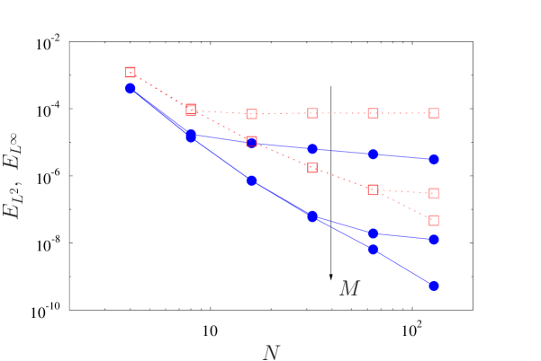
Figure 3: Dependence of (blue solid circles) the $L^{2}$ error (38a) and (red empty squares) $L^{\infty}$ error (38b) on the number of grid points $N$ for different truncation levels $M=10,15,20$. The trend with the increase of $M$ is indicated by an arrow.

We now proceed to validate the approach described above and do so by comparing the numerical approximation of (27) for $p=2$ with the exact solution (28b). There are two numerical parameters in the problem, namely, the number of terms $M$ after which the Fourier series in (34) is truncated and the number of gridpoints $N$ in the Gauss-Legendre quadrature used to approximate (37). Denoting the solution obtained numerically with these parameters $\gamma^{M,N}_{2}$, we consider the following two error measures

$$E_{L^{2}} :=\|\gamma^{M,N}_{2}-\gamma_{2}\|_{L^{2}(0,1)},$$ (38a)

$$E_{L^{\infty}} :=\|\gamma^{M,N}_{2}-\gamma_{2}\|_{L^{\infty}(0,1)}.$$ (38b)

The dependence of these errors on the number of grid points $N$ for different truncation levels $M$ is shown in figure 3, where we see that provided $M$ is sufficiently large, the error measures (38a) and (38b) show, respectively, fourth-order and third-order rate of convergence with respect to grid refinement in the quadrature (spectral convergence is not achieved because of the presence of the square-root function in the integrand of (37)). In the computational results presented in the next section we use $N=2048$ (which gives a much finer resolution than used in figure 3), whereas the parameter $M$ is adjusted for different $p$ based on the data presented in figure 2 to ensure that errors due to truncation of the series in (34) remain at the level of the machine precision.

5 Results

In this section we present circulation densities obtained for different values of $p$ by approximating formula (27) as discussed in Section 4. Since the circulation densities are defined up to a multiplicative factor $\omega$, we normalize them such that the equilibrium configurations $L$ corresponding to different values of $p$, cf. (13), have the same total circulation equal to one. We will thus focus on the following normalized quantity

$$\widetilde{\gamma}_{p}(s):=\frac{\gamma_{p}(s)}{2p\int_{0}^{1}\gamma_{p}(s^{\prime})\,ds^{\prime}},\quad s\in[0,1],\ p=1,2,\dots$$ (39)

which is plotted for $p=1,2,\dots,10$ in figure 4(a). We recognize that the distributions obtained for $p=1$ and $p=2$ correspond to the exact solutions (28a) and (28b). It is interesting to note that, except for the case $p=1$, all circulation densities vanish at $s=0$ which corresponds to the center of rotation, a property which is not a priori guaranteed by the general inversion formula (11), but is evident in the form of (27). We also observe that as $p$ increases the magnitude of $\widetilde{\gamma}_{p}(s)$ is reduced which is a consequence of the fact that since the circulation of the entire equilibrium configuration is fixed, the circulations of the individual sheets decrease as their number $p$ goes up. In addition, in figure 4(a) we observe that there is no apparent difference between the distributions $\widetilde{\gamma}_{p}(s)$ obtained for $p$ even and $p$ odd, and that these distributions become more skewed towards the outer endpoint of the sheet at $s=1$ as $p$ increases. This latter effect is further explored in figure 4(b) where we show the normalized circulation densities $\widetilde{\gamma}_{p}(s)$ corresponding to much higher values of $p=20,119,\dots,2000$. In this figure we observe that $\widetilde{\gamma}_{p}(s)\rightarrow 0$ as $p\rightarrow\infty$ for all values of $s\in[0,1-\epsilon)$, $\epsilon>0$, except for a small neighborhood near the endpoint $s=1$ in which the entire circulation of the vortex sheet becomes localized in the form of a few sign-changing oscillations. In order to shed further light on this behavior, in figure 5 we show the quantity $2p\,\widetilde{\gamma}_{p}(s)$ in a small neighborhood of the right endpoint $s=1$, corresponding to $0.625\%$ of the entire interval $[0,1]$. We observe that in the limit $p\rightarrow\infty$ the dominant “wiggle” becomes steeper and more localized. The significance of this observation is discussed in the next, final section.

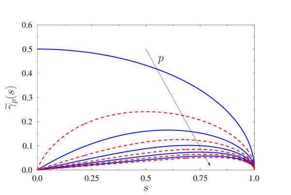
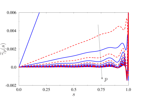
Figure 4: Normalized circulation densities $\widetilde{\gamma}_{p}(s)$, cf. (39), as functions of position $s\in[0,1]$ for (a) $p=1,2,\dots,10$ and (b) $p=20,119,\dots,2000$. Red dashed lines and blue solid lines correspond to, respectively, $p$ even and odd. The trend with the increase of $p$ is indicated by an arrow.

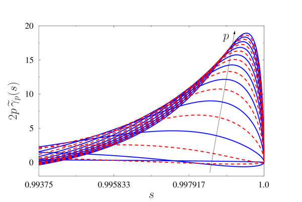
Figure 5: Rescaled normalized circulation densities $2p\,\widetilde{\gamma}_{p}(s)$ obtained for $p=20,119,\dots,2000$ in a small neighborhood of the right endpoint $s=1$. Red dashed lines and blue solid lines correspond to, respectively, $p$ even and odd. The trend with the increase of $p$ is indicated by an arrow.

6 Discussion and Conclusions

In this investigation we have considered the question of finding relative equilibria involving vortex sheets in 2D potential flows. By framing this question in terms of the Riemann-Hilbert problem in complex analysis we proposed a general two-step approach to finding such equilibria, where one first constructs a geometric configuration of vortex sheets which satisfies the compatibility conditions (9) and then finds the corresponding circulation densities by evaluating formula (11). The compatibility conditions ensure that the circulation densities vanish at all sheet endpoints, which is necessary for the velocity field to be everywhere well behaved, and additional symmetry arguments are used to ensure the circulation densities are real-valued. Using this approach together with analytical computations we constructed a family of rotating equilibria involving an even number $2p$ of radially-oriented straight segments revolving about a common center of rotation where they meet, cf. figure 1, which generalizes the well-known solution (1) corresponding to a single rotating vortex sheet. The circulation densities of the rotating sheets are given in closed form for the integral formula (27), the evaluation of which however requires a careful numerical approach described in Section 4. This construction was facilitated by a judicious choice of the geometric configuration $L$, cf. (13), consisting of $p$ bent sheets with endpoints at the vertices of a regular $2p$-gon whose midpoints touch at the center of rotation. As a result, it was not necessary to consider the center of rotation as a separate sheet endpoint, although the obtained circulation densities $\gamma_{p}(s)$ do vanish there (i.e., at $s=0$) for all $p>1$, cf. (27) and figure 4(a), meaning that the center of rotation may in fact be interpreted as a sheet endpoint when $p>1$. It is possible that these new equilibria could also be obtained using other methods, such as, e.g., conformal transformations based on the Schwarz-Christoffel map.

We found that in the limit of the equilibrium configurations consisting of a large number of sheets, i.e., when $p\rightarrow\infty$, the normalized circulation densities $\widetilde{\gamma}_{p}(s)$, cf. (39), vanish everywhere except for a vanishing neighborhood of the outer endpoint where the entire circulation of the sheet is localized in the form of a rapid oscillation with intensity increasing with $p$. Thus, the limiting configuration appears to have the form of a hollow vortex of unit radius bounded by a constant-density circular vortex sheet, which is also a well known equilibrium solution. It must be, however, emphasized that this limit ought to be considered in some suitable “weak” sense, rather than in the classical pointwise (uniform) sense. The reason is that in the neighborhood of $s=1$ the values of $2p\,\widetilde{\gamma}_{p}(s)$ diverge as $p\rightarrow\infty$ with the sequence approaching a singular distribution at $s=1$, cf. figure 5. This limiting distribution clearly does not belong to the Hölder space in which the circulation densities most be defined [18] and is also not consistent with conditions (8). Since both the relative equilibria constructed here and the hollow vortex with a vortex sheet are solutions of 2D Euler equations defined in a suitable distributional sense [16], we thus have a countably infinite sequence of distributional solutions of the first type converging to the solution of the second type which is characterized by a different topology. Understanding the precise mathematical sense of this convergence is an interesting open question.

Since our ansatz for the rotating equilibrium configurations involves an even number ($2p$) of segments, cf. figure 1, an interesting question concerns construction of equilibria consisting of an odd number of segments (such as, e.g., $\mathbin{\mathchoice{\kern 1.66666pt\raise 0.0pt\hbox{{\rotatebox{120.0}{\hbox to0.0pt{\hss\clipbox{0pt {} 0pt -}{$\displaystyle|$}\hss}}}\hbox to0.0pt{\hss\clipbox{0pt {} 0pt -}{$\displaystyle|$}\hss}{\rotatebox{-120.0}{\hbox to0.0pt{\hss\clipbox{0pt {} 0pt -}{$\displaystyle|$}\hss}}}}\kern 1.66666pt}{\kern 1.66666pt\raise 0.0pt\hbox{{\rotatebox{120.0}{\hbox to0.0pt{\hss\clipbox{0pt {} 0pt -}{$\textstyle|$}\hss}}}\hbox to0.0pt{\hss\clipbox{0pt {} 0pt -}{$\textstyle|$}\hss}{\rotatebox{-120.0}{\hbox to0.0pt{\hss\clipbox{0pt {} 0pt -}{$\textstyle|$}\hss}}}}\kern 1.66666pt}{\kern 1.49998pt\raise 0.0pt\hbox{{\rotatebox{120.0}{\hbox to0.0pt{\hss\clipbox{0pt {} 0pt -}{$\scriptstyle|$}\hss}}}\hbox to0.0pt{\hss\clipbox{0pt {} 0pt -}{$\scriptstyle|$}\hss}{\rotatebox{-120.0}{\hbox to0.0pt{\hss\clipbox{0pt {} 0pt -}{$\scriptstyle|$}\hss}}}}\kern 1.49998pt}{\kern 1.38887pt\raise 0.0pt\hbox{{\rotatebox{120.0}{\hbox to0.0pt{\hss\clipbox{0pt {} 0pt -}{$\scriptscriptstyle|$}\hss}}}\hbox to0.0pt{\hss\clipbox{0pt {} 0pt -}{$\scriptscriptstyle|$}\hss}{\rotatebox{-120.0}{\hbox to0.0pt{\hss\clipbox{0pt {} 0pt -}{$\scriptscriptstyle|$}\hss}}}}\kern 1.38887pt}}$). In such case, the center of rotation would need to be treated as a separate endpoint resulting in more complicated form of the compatibility conditions (9). However, we expect that in the limit of a large number of segments the behavior of such hypothetical equilibria would be similar to what we observed here in figures 4(b) and 5. A related interesting question concerns the existence of equilibria with less symmetry. In this context, we have considered the following configuration of three sheets

$$L=[-1,-\alpha]\ \cup\ [\alpha,1]\ \cup\ [-i\beta,i\beta]$$ (40)

defined for some $\alpha,\beta>0$ and observed that for all $\alpha\in(0,1)$ there exists $\beta=\beta(\alpha)$ such that this configuration forms an equilibrium. Moreover, $\beta(\alpha)\rightarrow 1$ as $\alpha\rightarrow 0$, meaning that in this limit configuration (40) approaches the equilibrium corresponding to $p=2$, cf. (28b) and figure 1(b). Discussion of this and other equilibria generalizing the configurations found in this study and possibly involving curved vortex sheets is deferred to a future publication.

Another, more fundamental, question concerns equilibria in a translating frame of reference. Using $f(z)=U$ in (9) it can be shown that for the geometric configuration (13) already the first compatibility condition is violated, i.e., $C_{0}\neq 0$, demonstrating that this configuration cannot form a translating equilibrium. While in the present study configuration (13) was proposed based on evidence from numerical experiments, in more general situations geometric configurations $L$ which form equilibria can be found by solving equations (9) treated as a problem defining $L$. Yet another interesting problem is the stability of the equilibrium configurations discovered here. We plan to address some of these questions in the near future.

Appendix A Evaluation of Singular Integrals (36)

For modest values of $k$ the principal-value integrals (36a)–(36b) can be evaluated symbolically, for example, using the software package Maple. Denoting $X:=\cos\phi$ and $Y:=\frac{\operatorname{arcCoth}\left(\frac{1}{\sin\phi}\right)}{\sin\phi}$, where $\phi\in[0,\pi/2]$, these integrals take the form

$$\Psi_{0}(\cos\eta) =Y,$$ (41a)

$$\Psi_{2}(\cos\eta) =(2X^{2}-1)Y+2,$$ (41b)

$$\Psi_{4}(\cos\eta) =(8X^{4}-8X^{2}+1)Y+8X^{2}-\frac{8}{3},$$ (41c)

$$\Psi_{6}(\cos\eta) =(32X^{6}-48X^{4}+18X^{2}-1)Y+32X^{4}-\frac{80X^{2}}{3}+\frac{46}{15},$$ (41d)

$$\dots$$

$$\Phi_{0}(\cos\eta) =\frac{\pi}{2},$$ (42a)

$$\Phi_{2}(\cos\eta) =\pi X^{2},$$ (42b)

$$\Phi_{4}(\cos\eta) =\pi(4X^{4}-2X^{2}),$$ (42c)

$$\Phi_{6}(\cos\eta) =\pi(16X^{6}-16X^{4}+3X^{2}),$$ (42d)

$$\Phi_{8}(\cos\eta) =\pi(64X^{8}-96X^{6}+40X^{4}-4X^{2}),\phantom{==========}$$ (42e)

$$\dots$$

where due to the properties of the function $f(\theta)$ we considered only even values of $k$. Evidently, the expressions in (41) can be represented as $\Psi_{2m}(\phi)=p_{2m}(X)\,Y+r_{2m}(X)$ and as can be verified by inspection the polynomials $p_{2m}(X)$ and $r_{2m}(X)$ satisfy the following recursion relations

$$p_{2m+2}(X) =(4X^{2}-2)p_{2m}(X)-p_{2m-2}(X),\quad m\geqq 1,$$ (43a)

$$p_{0}(X) =1,\quad p_{2}(X)=2X^{2}-1,$$ (43b)

$$r_{2m+2}(X) =q_{2m+2}(X)+s_{2m+2},$$ (43c)

$$q_{2m+2}(X) =(4X^{2}-2)r_{2m}(X)-r_{2m-2}(X),\quad m\geqq 1,$$ (43d)

$$q_{0}(X) =0,\quad q_{2}(X)=2,$$ (43e)

$$s_{2m+2} =\frac{N_{2m+2}}{D_{2m+2}},\quad N_{2m}=(-1)^{m}\,4,$$ (43f)

$$D_{2m+2} =2D_{2m}-D_{2m-2}+8,\quad m\geqq 1,\quad D_{0}=3,\ D_{2}=1,$$ (43g)

where $s_{2m}$ are rational numbers whereas $D_{2m}$ and $N_{2m}$ are integers. Analogously, the expressions in (42) can be represented as $\Phi_{2m}(\phi)=\pi Q_{2m}(X)$ where the polynomials $Q_{2m}(X)$ follow the recursion relations

$$Q_{2m+2}(X) =(4X^{2}-2)Q_{2m}(X)-Q_{2m-2}(X),\quad m\geqq 2,$$ (44a)

$$Q_{2}(X) =X^{2},\quad Q_{4}(X)=4X^{4}-2X^{2},$$ (44b)

$$Q_{0}(X) =\frac{1}{2}.$$ (44c)

Finally, expressions (41)–(42) together with the recursion relations (43)–(44) make it possible to evaluate the principal-value integrals (36a)–(36b) for arbitrary values of $k$.

References

- [1] Mark J. Ablowitz and Athanassios S. Fokas. Complex Variables: Introduction and Applications. Cambridge University Press, Second edition, 2011.
- [2] Silas Alben. Simulating the dynamics of flexible bodies and vortex sheets. Journal of Computational Physics, 228(7):2587 – 2603, 2009.
- [3] H. Aref, P. K. Newton, M. A. Stremler, T. Tokieda, and D. L. Vainchtein. Vortex crystals. Advances in Applied Mechanics, 39:1–79, 2003.
- [4] Hassan Aref. Point vortex dynamics: A classical mathematics playground. Journal of Mathematical Physics, 48(6):065401, 2007.
- [5] G. R. Baker, P. G. Saffman, and J. S. Sheffield. Structure of a linear array of hollow vortices of finite cross-section. Journal of Fluid Mechanics, 74(3):469–476, 1976.
- [6] Andrea Barreiro, Jared Bronski, and Paul K. Newton. Spectral gradient flow and equilibrium configurations of point vortices. Proceedings of the Royal Society A: Mathematical, Physical and Engineering Sciences, 466(2118):1687–1702, 2010.
- [7] G. K. Batchelor. An Introduction to Fluid Dynamics. Cambridge University Press, Cambridge, 1967.
- [8] R. E. Caflisch, editor. Mathematical Aspects of Vortex Dynamics. SIAM, 1989.
- [9] P. A. Clarkson. Vortices and polynomials. Studies in Applied Mathematics, 123(1):37–62, 2009.
- [10] D. G. Dritschel. The stability and energetics of corotating uniform vortices. J. Fluid Mech., 157:95–134, 1985.
- [11] Federico Gallizio, Angelo Iollo, Bartosz Protas, and Luca Zannetti. On continuation of inviscid vortex patches. Physica D: Nonlinear Phenomena, 239(3):190 – 201, 2010.
- [12] T.Y. Hou, V.G. Stredie, and T.Y. Wu. Mathematical modeling and simulation of aquatic and aerial animal locomotion. Journal of Computational Physics, 225(2):1603 – 1631, 2007.
- [13] Marvin A. Jones. The separated flow of an inviscid fluid around a moving flat plate. Journal of Fluid Mechanics, 496:405–441, 2003.
- [14] J. R. Kamm. Shape and stability of two–dimensional vortex regions. PhD thesis, Caltech, 1987.
- [15] P. Luzzatto-Fegiz and C. H. K. Williamson. Stability of conservative flows and new steady-fluid solutions from bifurcation diagrams exploiting variational argument. Phys. Rev. Lett., 104:044504, 2010.
- [16] A. J. Majda and A. L. Bertozzi. Vorticity and Incompressible Flow. Cambridge University Press, 2002.
- [17] D. W. Moore, P. G. Saffman, and S. Tanveer. The calculation of some Batchelor flows: The Sadovskii vortex and rotational corner flow. The Physics of Fluids, 31(5):978–990, 1988.
- [18] N. I. Muskhelishvili. Singular Integral Equations. Boundary Problems of Function Theory and Their Application to Mathematical Physics. Dover, 2nd edition edition, 2008.
- [19] Paul K Newton. Point vortex dynamics in the post-Aref era. Fluid Dynamics Research, 46(3):031401, may 2014.
- [20] Paul K Newton and George Chamoun. Construction of point vortex equilibria via brownian ratchets. Proceedings of the Royal Society A: Mathematical, Physical and Engineering Sciences, 463(2082):1525–1541, 2007.
- [21] Kevin A. O’Neil. Relative equilibria of vortex sheets. Physica D: Nonlinear Phenomena, 238(4):379 – 383, 2009.
- [22] Kevin A. O’Neil. Collapse and concentration of vortex sheets in two-dimensional flow. Theoretical and Computational Fluid Dynamics, 24(1):39–44, Mar 2010.
- [23] Kevin A. O’Neil. Dipole and multipole flows with point vortices and vortex sheets. Regular and Chaotic Dynamics, 23:519–529, 2018.
- [24] Kevin A. O’Neil. Relative equilibria of point vortices and linear vortex sheets. Physics of Fluids, 30(10):107101, 2018.
- [25] R. T. Pierrehumbert. A family of steady, translating vortex pairs with distributed vorticity. Journal of Fluid Mechanics, 99(1):129–144, 1980.
- [26] H. C. Pocklington. The configuration of a pair of equal and opposite hollow straight vortices of finite cross-section, moving steadily through fluid. Proc. Camb. Phil. Soc., 8:178–187, 1895.
- [27] V. S. Sadovskii. Vortex regions in a potential stream with a jump of Bernoulli’s constant at the boundary. Appl. Math. Mech., 35:729, 1971.
- [28] P. G. Saffman. Vortex Dynamics. Cambridge Monographs on Mechanics and Applied Mathematics. Cambridge University Press, Cambridge, 1992.
- [29] P. G. Saffman and R. Szeto. Equilibrium shapes of a pair of equal uniform vortices. Phys Fluids, 23:2339–2342, 1980.
- [30] Ratnesh K. Shukla and Jeff. D. Eldredge. An inviscid model for vortex shedding from a deforming body. Theoretical and Computational Fluid Dynamics, 21(5):343, Jul 2007.
- [31] H. Telib and L. Zannetti. Hollow wakes past arbitrarily shaped obstacles. Journal of Fluid Mechanics, 669:214–224, 2011.
- [32] Yieh-Hei Wan. Desingularizations of systems of point vortices. Physica D: Nonlinear Phenomena, 32(2):277 – 295, 1988.