Superfast Approximate
Least Squares Solution of a Highly
Overdetermined Linear System of Equations

Abstract

With a high probability (whp) the Sarlòs randomized algorithm of 2006 outputs a nearly optimal least squares solution of a highly overdetermined linear system of equations. We propose its simple deterministic variation that computes such a solution for a random input whp and therefore computes it deterministically for a large input class. Unlike the Sarlòs original algorithm our variation performs computations at sublinear cost or, as we say, superfast, that is, by using much fewer memory cells and arithmetic operations than an input matrix has entries. Our extensive tests are in good accordance with this result.

Key Words:

Overdetermined Linear Systems, Least Squares Solution, Superfast algorithms

2020 Math. Subject Classification:

65Y20, 65F05, 68Q25, 68W25

1 Introduction

The Linear Least Squares Problem (LLSP). The computation of a least squares solution to a highly overdetermined linear system of equations is a hot research subject, fundamental for Matrix Computations and Big Data Mining and Analysis (see the books [LH95] and [B96], more recent works [DMM06], [RT08], [BD09], [AMT10], [DMMS11], [M11], [LWM18], and the references therein). By following Björk’s book [B15] we call this task Linear Least Squares Problem and hereafter refer to it as LLSP. Some authors call it differently, e.g., Least Squares Approximation Problem [M11].

The matrices that define Big Data are frequently so immense that realistically one can access only a tiny fraction of their entries and thus must perform computations at sublinear cost or, as we say, superfast – by using much fewer memory cells and arithmetic operations than an input matrix has entries.

Our progress. Unfortunately the output of any superfast algorithm is extremely far from the solution to LLSP problem on the worst case inputs (see the beginning of Section 3), but we circumvent this problem based on a simple new application of the Sarlòs randomized algorithm of [S06]. This algorithm multiplies an input matrix of LLSP by a rectangular multiplier, so that the resulting LLSP has a much smaller size and can be readily solved superfast. The original input matrix can be assumed to be orthogonal without loss of generality, and for the multiplier one can choose a rectangular Gaussian random matrix, that is, a matrix filled with independent identically distributed Gaussian (aka normal) random variables. Hereafter we call such a matrix just Gaussian.

Its product with an orthogonal matrix is Gaussian, by virtue of orthogonal invariance, and Sarlòs proves that the solution of the resulting LLSP closely approximates the solution of the original LLSP whp. Now we observe that his result still holds for the solution of the dual LLSP, with a Gaussian input matrix and any orthogonal multiplier (see our Theorem 3.1).

Is this result of any interest? Yes, because by fixing a sparse multiplier we devise a superfast deterministic algorithm that computes a nearly optimal solution to LLSP for a large class of highly overdetermined inputs.

We say “a large class”, but could have argued that in a sense this holds for most inputs, because the nearly optimal solution is obtained for Gaussian input whp and because such a claim is in a good accordance with the results of our tests for both synthtic and real world inputs.

Of course one would prefer to solve LLSP superfast for all inputs, but

(a) this is impossible,

(b) the user should be satisfied even if the problem is solved just for the input class of her/his interest,

(c) Theorem 3.1 implies that this outcome is quite likely for many applications, and

(d) the results of our extensive tests with both synthetic and real world inputs are in good accordance with that theorem.

For a simple summary: it is impossible to ensure superfast solution for ANY INPUT, but we describe a simple superfast algorithm that works for MANY INPUTS, and we provide evidence to this by proving that the algorithm works whp for a random input and by supporting it with extensive numerical tests.

Related works. Our present result is just a new example of dual matrix algorithms, which we earlier devised, analyzed, and tested for other fundamental matrix computations such as Gaussian elimination with no pivoting in [PQY15] and [PZ17] and Low Rank Approximation (LRA) of a matrix in [PZ16], [PLSZ16], [PLSZ17], [PLSZ20], [PLSZa], [PLa], [LPSa], and [Pa]. We hope that these studies together with our present work will motivate research efforts towards devising superfast deterministic algorithms for matrix computations that would work for large classes of inputs, thus providing an alternative to the known randomized algorithms that whp solve these probems for all inputs but perform much slower.

Organization of the paper. In the next section we recall the LLSP and its randomized approximate solution by Sarlòs of [S06]. We present our superfast variation of his algorithm in Section 3. In Section 4, the contribution of the first author, we cover our numerical tests.

2 Randomized Approximate Solution of an Overdetermined Linear System of Equations

Problem 2.1.

[Least Squares Solution of an Overdetermined Linear System of Equations (LLSP).] Given two integers $m$ and $d$ such that $1\leq d<m$, a matrix $A\in\mathbb{R}^{m\times d}$, and a vector ${\bf b}\in\mathbb{C}^{m}$, compute a vector ${\bf x}\in\mathbb{R}^{d}$ that minimizes the spectral norm $||A{\bf x}-{\bf b}||$ or equivalently computes the subvector ${\bf x}=(y_{j})_{j=0}^{d-1}$ of the vector

$${\bf y}=(y_{j})_{j=0}^{d}={\rm argmin}_{\bf v}~{}||M{\bf v}||~{}{\rm such~{}that}~{}M=(A~{}|~{}{\bf b})~{}{\rm and}~{}{\bf v}=\begin{pmatrix}{\bf x}\\ -1\end{pmatrix}.$$ (2.1)

The minimum norm solution to this problem is given by the vector ${\bf x}=A^{+}{\bf b}$ for $A^{+}$ denoting the Moore–Penrose pseudo inverse of $A$; $A^{+}{\bf b}=(A^{*}A)^{-1}A^{*}{\bf b}$ if a matrix $A$ has full rank $d$.

Algorithm 2.1.

(Randomized Approximate Solution of LLSP from [S06].)

Input:

An $m\times(d+1)$ matrix $M$.

Output:

A vector ${\bf x}\in\mathbb{R}^{d}$ approximating a solution of Problem 2.1.

Initialization:

Fix an integer $s$ such that $d\leq s\ll m$.

Computations:

1. Generate a matrix $F\in\mathbb{R}^{s\times m}$.

2. Compute a solution ${\bf x}$ of Problem 2.1 for the $s\times(d+1)$ matrix $FM$.

Clearly the transition to an input matrix $FM$ simplifies Problem 2.1 because its size decreases, and the simplification is dramatic where $s\ll m$, while the following theorem shows that the algorithm still outputs nearly optimal approximate solution to Problem 2.1 for $M$ whp if ${\sqrt{s}}~{}F$ is in the linear space $\mathcal{G}^{s\times m}$ of $s\times m$ Gaussian matrices.

Theorem 2.1.

(Error Bound for Algorithm 2.1. See [S06] or [W14, Theorem 2.3].) Let us be given two integers $s$ and $d$ such that $0<d\leq s$, two matrices $M\in\mathbb{R}^{m\times(d+1)}$ and Gaussian $F\in\mathcal{G}^{s\times m}$, and two tolerance values $\gamma$ and $\epsilon$ such that

$$0<\gamma<1,~{}0<\epsilon<1,~{}{\rm and}~{}s=\Big{(}d+\log\Big{(}\frac{1}{\gamma}\Big{)}\Big{)}~{}\frac{\eta}{\epsilon^{2}}$$ (2.2)

for a constant $\eta$. Then

$${\rm Probability}\Big{\{}1-\epsilon\leq\frac{1}{\sqrt{s}}~{}\frac{||FM{\bf y}||}{||M{\bf y}||}\leq 1+\epsilon~{}{\rm for~{}all~{}vectors}~{}{\bf y}\neq{\bf 0}\Big{\}}\geq 1-\gamma.$$ (2.3)

The computation of the matrix $FM$ involves order of $dsm\geq d^{2}m$ flops; for $m\gg s$ this dominates the overall arithmetic computational cost of the solution of Problem 2.1.

The current record upper estimate for this cost is $O(d^{2}m)$ (see [CW17], [W14, Section 2.1]), while the record lower bound of [CW09] has order $(m+d)s\epsilon^{-1}\log(md)$ provided that the relative output error norm is within a factor of $1+\epsilon$ from its minimal value.

3 Superfast Dual LLSP

Any superfast algorithm for LLSP misses an input entry $m_{i,j}$ for some pair $i$ and $j$; therefore for its output the norm $||M{\bf y}||$ exceeds the norm $||M{\bf x_{\rm optimal}}||$by arbitrarily large factor for the worst case input $M$. Indeed modification of $m_{i,j}$ does not change the output of such an algorithm but can dramatically change an optimal solution to the LLSP.

The argument can be immediately extended to randomized algorithms, and so no superfast deterministic or randomized algorithm can solve Problem 2.1 for all inputs. E.g., the randomized Algorithm 2.1 outputs nearly optimal solution of LLSP whp for any input, but it is not superfast. Now we can repeat our argument in the Introduction that the user would be happy even if the problem is solved just for a class of inputs of her/his interest, and this should motivate devising superfast algorithms that would solve LLSP for a large class of inputs. Our next theorem implies that a simple variation of Algorithm 2.1 is quite likely to do this.

Namely, by virtue of that theorem the algorithm still outputs a nearly optimal solution of Problem 2.1 whp in the case of a random Gaussian input $M$ and any properly scaled unitary multiplier $F$. By choosing a proper sparse multiplier we arrive at a superfast algorithm.

Theorem 3.1.

[Error Bounds for Dual LLSP.] Suppose that we are given three integers $s$, $m$, and $d$ such that $0<d\leq s<m$, and two tolerance values $\gamma$ and $\epsilon$ satisfying (2.2). Define a unitary matrix $Q_{s,m}\in\mathbb{R}^{s\times m}$ and a matrix $G_{m,d+1}\in\mathcal{G}^{m\times(d+1)}$ and write

$$F:=a~{}Q_{s,m}~{}{\rm and}~{}M:=b~{}G_{m,d+1}$$ (3.1)

for two scalars $a$ and $b$ such that $ab\sqrt{s}=1$. Then

$${\rm Probability}\Big{\{}1-\epsilon~{}\leq\frac{||FM{\bf z}||}{||M{\bf z}||}\leq 1+\epsilon~{}{\rm for~{}all~{}vectors}~{}{\bf z}\neq{\bf 0}\Big{\}}\geq 1-\gamma.$$

Proof.

The claim follows from Theorem 2.1 because the $s\times(d+1)$ matrix $\frac{1}{ab}FM$ is Gaussian by virtue of unitary invariance of Gaussian matrices. ∎

The theorem shows that for a Gaussian matrix $M$ and any properly scaled unitary matrix $F$ of (3.1) Algorithm 2.1 outputs a solution of Problem 2.1 that whp is optimal up to a factor lying in the range $[1-\epsilon,1+\epsilon]$.

4 Numerical Tests for LLSP

In this section we present the results of our tests of Algorithm 2.1 for both synthetic and real-world data. We worked with random unitary multipliers, let ${\bf x}:=\operatorname*{arg\,min}_{\bf u}||FA{\bf u}-F{\bf b}||$, and computed the relative residual norm

$$\frac{||A{\bf x}-{\bf b}||}{\min_{\bf u}||A{\bf u}-{\bf b}||}.$$

In our tests these ratios quite closely approximated 1 from above.

We used the following random scaled unitary multipliers $F\in\mathbb{R}^{s\times m}$:

(i) full rank $s\times m$ submatrices of $m\times m$ random permutation matrices,

(ii) ASPH matrices from [PLSZ20] and [PLSZa], which we output after performing just the first three recursive steps out of $\log_{2}{m}$ steps involved into the generation of the matrices of subsampled randomized Hadamard thansform, and

(iii) block permutation matrices formed by filling $s\times m$ matrices with $c=m/s$ identity matrices, each of size $s\times s$, and performing random column permutations; we have chosen $c=8$ to match the computational cost of the application of ASPH multipliers.

For comparison we also included the test results with $s\times m$ Gaussian multipliers.

We performed our tests on a machine with Intel Core i7 processor running Windows 7 64bit; we invoked the lstsq function from Numpy 1.14.3 for solving the LLSPs.

4.1 Synthetic Input Matrices

For synthetic inputs, we generated input matrices $A\in\mathbb{R}^{m\times d}$ by following (with a few modifications) the recipes of extensive tests in [AMT10], which compared the running time of the regular LLSP problems and the reduced ones with WHT, DCT, and DHT pre-processing.

We used input matrices $A$ of size $4096\times 50$ and $16834\times 100$ being either Gaussian matrices or random ill-conditioned matrices. We generated the input vectors ${\bf b}=\frac{1}{||A{\bf w}||}A{\bf w}+\frac{0.001}{||{\bf v}||}{\bf v}$, where ${\bf w}$ and ${\bf v}$ were random Gaussian vectors of size $d$ and $m$, respectively, and so ${\bf b}$ was in the range of $A$ up to a smaller term $\frac{0.001}{||{\bf v}||}{\bf v}$.

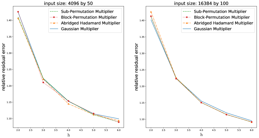
Figure 1 displays the test results for Gaussian input matrices.

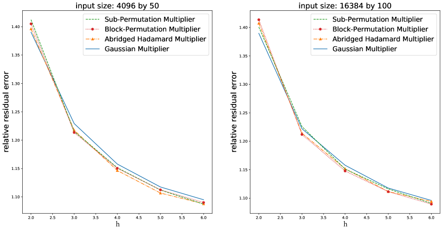
Figure 2 displays the test results for ill-conditioned random inputs defined by their SVD $A=U\Sigma V^{*}$ where the unitary matrices $U$ and $V$ of singular vectors were given by the Q factors in QR-factorization of two independent Gaussian matrices and where $\Sigma=\operatorname{diag}(\sigma_{j})_{j}$ with $\sigma_{j}=10^{5-j}$ for $j=1,2\dots,14$ and $\sigma_{j}=10^{-10}$ for $j>14$.

Our input matrices $A$ were highly over-determined, having many more rows than columns. We have chosen $s=dh$, $h=2,3,4,5,6$ for the multipliers $F$. By decreasing the ratio $h=s/d$ and therefore the integer $s$ we would accelerate the computations of our algorithm, but we had to keep it large enough in order to yield accurate solution.

We performed 100 tests with 100 random multipliers for every triple of the input class, multiplier class, and test sizes (cf. (2.2)) and computed the mean of the 100 relative residual norms of the output.

We display the test results in Figures 1 and 2 with ratio $h$ marked on the horizontal axis. The tests show that our multipliers were consistently effective for random matrices. The performance was not affected by the conditioning of input matrices.

Figure 1: Relative residual norm in tests with Gaussian inputs

Figure 2: Relative residual norm in tests with ill-conditioned random inputs

4.2 Red Wine Quality Data and California Housing Prices Data

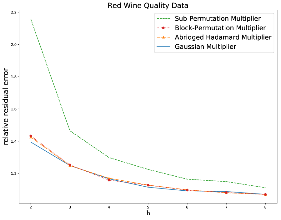
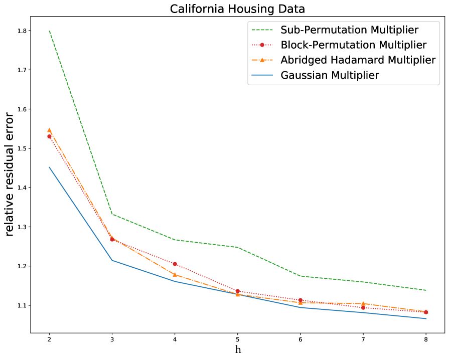
In this subsection we present the test results for real world inputs, namely the Red Wine Quality Data and California Housing Prices Data. For each triple of the datasets, multiplier type and multiplier size, we repeated the test for 100 random multipliers and computed the mean relative residual norm. The results for these two input classes are displayed in Figures 3 and 4.

11 physiochemical feature data of the Red Wine Quality Data such as fixed acidity, residual sugar level, and pH level were the input variables in our tests and one sensory data wine quality were the output data; the tests covered 1599 variants of the Portuguese ”Vinho Verde” wine. See further information in [CCAMR09]. This dataset is often applied in regression tests that use physiochemical data of a specific wine in order to predict its quality, and among various types of regression LLSP algorithms are considered a popular choice.

From this dataset we constructed a $2048\times 12$ input matrix $A$ with each row representing one variant of red wine, and with columns consisting of a bias column and eleven physiochemical feature columns. The input vector ${\bf b}$ is a vector consisting of the wine quality level (between 0 and 10) for each variant. We kept the 1599 rows of the original data, padded the rest of the rows with zeros, and performed a full row permutation of $A$.

The California Housing Prices data appeared in [PB97] and were collected from the 1990 California Census, including 9 attributes for each of the 20,640 Block Groups observed. This dataset is used for regression tests in order to predict the median housing value of a certain area given collected information of this area, such as population, median income, and housing median age.

We randomly selected 16,384 observations from the dataset in order to construct an independent input matrix $A_{0}$ of size $16384\times 8$ and a dependent input vector ${\bf b}\in\mathbb{R}^{16384}$. Furthermore, we augmented $A_{0}$ with a single bias column, i.e. $A=\begin{bmatrix}A_{0}&{\bf 1}\end{bmatrix}$.

We computed approximate solutions by applying the algorithm supporting Theorem 3.1 and using our multipliers. Figure 3 and 4 show that the resulting solution was almost as accurate as the optimal solution. Moreover, using Gaussian multipliers rather than our sparse multipliers only enabled a marginal decrease of relative residual norm.

Figure 3: Relative residual norm in tests with Red Wine Quality Data

Figure 4: Relative residual norm in tests with California Housing Prices Data

Acknowledgements: Our work was supported by NSF Grants CCF–1563942 and CCF–1733834 and PSC CUNY Award 69813 00 48.