A cost-reducing partial labeling estimator in text classification problem

Abstract

We propose a new approach to address the text classification problems when learning with partial labels is beneficial. Instead of offering each training sample a set of candidate labels, we assign negative-oriented labels to the ambiguous training examples if they are unlikely fall into certain classes. We construct our new maximum likelihood estimators with self-correction property, and prove that under some conditions, our estimators converge faster. Also we discuss the advantages of applying one of our estimator to a fully supervised learning problem. The proposed method has potential applicability in many areas, such as crowd-sourcing, natural language processing and medical image analysis.

1 Introduction

In some circumstances, the process of labeling is distributed among less-than-expert assessors. With the fact that some data may belong to several classes by nature, their labeling for hundreds of pictures, texts, or messages a day is error-prone. The invention of partial labeling seeks to remedy the labor: instead of assigning one or some exact labels, the annotators can offer a set of possible candidate solutions for one sample, thus providing a buffer against potential mistakes [1, 4, 8, 16, 17, 26]; Other partial labeling settings involve repeated labeling to filter out noises, or assessing the quality of the labelers [18,22] to enhance the reliability of the models.

As the data size in companies such as FANG(Facebook, Amazon, Netflix, Google) constantly reaches the magnitude of Petabyte, the demand for quick, yet still precise labeling is ever growing. Viewing some practices, the partial labeling frameworks that we know of exhibit some limitations. For instance, in a real-world situation concerning NLP, if the task is to determine the class/classes of one article, an annotator with a bachelor degree of American literature might find it difficult to determine if an article with words dotted with ’viscosity’, ’gradient’, and ’Laplacian’ etc. belongs to computer science, math, physics, chemistry, or none of the classes above. As a result, the annotator might struggle within some limited amount of time amid a large pool of label classes and is likely to make imprecise choices even in a lenient, positive-oriented partial labeling environment. Another issue is the cost. Repeated labeling and keeping track of the performance of each labeler may be pricey, and the anonymity of the labelers can raise another barrier wall to certain partial labeling approaches.

Taking into consideration the real world scenarios, we present a new method to tackle the problem of how to gather at a large scale partially correct information from diverse annotators, while remaining efficient and budget-friendly. Still taking the above text classification problem as the example. Although that same annotator might not easily distinguish which categories the above-mentioned article belongs to, in a few seconds he/she can rule out the possibility the article is related to cuisines, TV-entertainment, or based on his/her own expertise, novels. In our partial label formulation, the safe choices, crossed-off categories labeled by annotators can still be of benefit. Furthermore, when contradictory labels are marked on one training sample and the identities of the labelers unknown, our introduced self-correcting estimator can select, and learn from the categories where the labels agree.

Based on this, we propose a new way to formulate partial labeling. For some documents, instead of having the exact labels, not belonging to certain classes is the information provided. To make use of both kinds of data, we propose two maximum likelihood estimators, one of which has a self-correction property to estimate the distribution of each classes. By making both type of labeled data contribute in the training process, we proved that our estimators converge faster than traditional Naive Bayes estimator. We finally find a way to apply our method to some only positive labeled data set, which is identified as a fully supervised learning problem, and achieve a better result compared to the traditional Naive Bayes.

The rest of this paper is organized as follows. Section 2 introduces the related works about text classification and partial labeling. Section 3 introduces the formulation of this problem, and conclude the result of traditional Naive Bayes estimator. Section 4 introduces the main results of our estimator, as well as how to apply it in fully supervised learning problem. Section 5 reports experimental results of comparative studies. Finally, Section 6 concludes the paper and discusses future research issues.

2 Related work

The text classification problem is seeking a way to best distinguish different types of documents[5, 12]. Being a traditional natural language processing problem, one needs to make full use of the words and sentences, converting them into various input features, and applying different models to process training and testing. A common way to convert words into features is to encoding them based on the term frequency and inverse document frequency, as well as the sequence of the words. There are many results about this, for example, tf-idf[19] encodes term $t$ in document $d$ of corpus $D$ as:

$$tfidf(t,d,D)=tf(t,d)\cdot idf(t,D),$$

where $tf(t,d)$ is defined as term frequency, it can be computed as $tf(t,d)=\frac{|{t:t\in d}|}{|d|}$, and $idf(t,D)$ is defined as inverse document frequency, it can be computed as $idf(t,D)=\log\frac{|D|}{|\{d\in D:t\in d\}|}$. We also have n-gram techniques, which first combines $n$ nearest words together as a single term, and then encodes it with tf-idf. Recently, instead of using tf-idf, [21] defines a new feature selection score for text classification based on the KL-divergence between the distribution of words in training documents and their classes.

A popular model to achieve our aim is to use Naive Bayes model[6, 11], the label for a given document $d$ is given by:

$$label(d)=\operatorname*{argmax}_{j}P(C_{j})P(d|C_{j}),$$

where $C_{j}$ is the $j$-th class. For example, we can treat each class as a multinomial distribution, and the corresponding documents are samples generated by the distribution. With this assumption, we desire to find the centroid for every class, by either using the maximum likelihood function or defining other different objective functions[2] in both supervised and unsupervised learning version[7]. Although the assumption of this method is not exact in this task, Naive Bayes achieves high accuracy in practical problems.

There are also other approaches to this problem, one of which is simply finding linear boundaries of classes with support vector machine[9, 3]. Recurrent Neural Network (RNN)[15, 23] combined with word embedding is also a widely used model for this problem.

In real life, one may have different type of labels[14], in which circumstance, semi-supervised learning or partial-label problems need to be considered [4]. There are several methods to encode the partial label information into the learning framework. For the partial label data set, one can define a new loss combining all information of the possible labels, for example, in [17], the authors modify the traditional $L^{2}$ loss

$$L(w)=\frac{1}{n+m}\left[\sum_{i=1}^{n}l(x_{i},y_{i},w)+\sum_{i=1}^{m}l(x_{i},Y_{i},w)\right],$$

where $Y_{i}$ is the possible label set for $x_{i}$ and $l(x_{i},Y_{i},w)$ is a non-negative loss function, and in [4], they defined convex loss for partial labels as:

$$L{{}_{\Psi}}(g(x),y)=\Psi(\frac{1}{|y|}{\sum_{a\in y}g_{a}(x)})+\sum_{a\notin y}\Psi(-g_{a}(x)),$$

where $\Psi$ is a convex function, $y$ is a singleton, and $g_{a}(x)$ is a score function for label $a$ as input $x$. A modification of the likelihood function is as well an approach to this problem and [8] gives the following optimization problem using Naive Bayes method

$$\theta^{*}=\arg\max_{\theta}\sum_{i}\sum_{y_{i}\in S_{i}}p(y|x_{i},\theta)$$

where $S_{i}$ is the possible labels for $x_{i}$.

Meanwhile, the similarity of features among data could be considered to give a confidence of each potential labels for a certain data. In [24], K nearest neighbor (KNN) is adopted to construct a graph structure with the information of features. While in [14] Rocchio and K-means clustering are used.

3 Formulation

3.1 General Setting

Consider a classification problem with independent sample $x\in S$ and class set $C$, where $C=\{C_{1},C_{2},...,C_{k}\}$. We are interested in finding our estimator:

$$\hat{y}=f(x;\theta)=(f_{1}(x;\theta),f_{2}(x;\theta),...,f_{k}(x;\theta))$$

for $y$, where $\theta=\{\theta_{1},\theta_{2},...,\theta_{m}\}$ is the parameter, and $f_{i}(x;\theta)$ is the likelihood function of sample $x$ in class $C_{i}$. Now assuming that in training set, we have two types of dataset $S_{1}$ and $S_{2}$, such that $S=S_{1}\cup S_{2}$:

1. dataset $S_{1}$: we know exactly that sample $x$ is in a class, and not in other classes. In this case, define: $y=(y_{1},y_{2},...,y_{k})$, if $x$ is in class $C_{i}$, then $y_{i}=1$. Notice that if this is a single label problem, then we have: $\sum_{i=1}^{k}y_{i}=1$.

2. dataset $S_{2}$: we only have the information that sample $x$ is not in a class, then $y_{i}=0$. In this case, define: $z=(z_{1},z_{2},...,z_{k})$, if $x$ is not in class $C_{i}$, we have $z_{i}=1$.

To build the model, we define the following likelihood ratio function and lihoodhood function:

$$L_{1}(\theta)=\prod_{x\in S_{1}}\prod_{i=1}^{k}f_{i}(x;\theta)^{y_{i}}\prod_{x\in S_{2}}\prod_{i=1}^{k}f_{i}(x;\theta)^{\frac{1-z_{i}}{k-\sum_{j\neq i}z_{j}}}.$$ (3.1)

$$L_{2}(\theta)=\prod_{x\in S}\frac{\prod_{i=1}^{k}f_{i}(x;\theta)^{y_{i}(x)+t}}{\prod_{i=1}^{k}f_{i}(x;\theta)^{z_{i}(x)}}=\prod_{x\in S}{\prod_{i=1}^{k}f_{i}(x;\theta)^{y_{i}(x)-z_{i}(x)+t}}.$$ (3.2)

The $t$ in $L_{2}$ satisfy $t>1$, which is a parameter to avoid non-convexity.

The intuition of $L_{1}$ is to consider the sample labeled $z_{i}=1$ has equal probability to be labeled in the other classes, each of the classes will have probability $\frac{1-z_{i}}{k-\sum_{j\neq i}z_{j}}.$ And the intuition of $L_{2}$ is to consider this in a likelihood ratio way, the $z_{i}=1$ labeled sample will have negative affection for class $C_{i}$, so we put it in the denominator. With $t>1$, all the terms in denominator will finally be canceled out, so that even $f_{i}(x;\theta)=0$ for some sample $x\in S$ will not cause trouble. Another intuition for $L_{2}$ is that, it can be self-correct the repeated data, which has been labeled incorrectly.

Take logarithm for both side, we obtain the following functions:

$$\log(L_{1}(\theta))=\sum_{x\in S_{1}}\sum_{i=1}^{k}y_{i}(x)\log{f_{i}(x,\theta)}+\sum_{x\in S_{2}}\sum_{i=1}^{k}{\frac{1-z_{i}}{k-\sum_{j\neq i}z_{j}}}\log{f_{i}(x,\theta)},$$ (3.3)

and

$$\log(L_{2}(\theta))=\sum_{x\in S}\sum_{i=1}^{k}(y_{i}(x)+t-z_{i}(x))\log{f_{i}(x,\theta)}.$$ (3.4)

We would like to find our estimator $\hat{\theta}$ such that (3.4) or (3.3) reaches maximum.

3.2 Naive Bayes classifier in text classification problem

For Naive Bayes model. Let class $C_{i}$ with centroid $\theta_{i}=(\theta_{i_{1}},\theta_{i_{2}},...,\theta_{i_{v}}),$ where $v$ is the total number of the words and $\theta_{i}$ satisfies: $\sum_{j=1}^{v}\theta_{i_{j}}=1$. Assuming independence of the words, the most likely class for a document $d=(x_{1},x_{2},...,x_{v})$ is computed as:

$$label(d) = \operatorname*{argmax}_{i}P(C_{i})P(d|C_{i})$$

$$= \operatorname*{argmax}_{i}P(C_{i})\prod_{j=1}^{v}(\theta_{i_{j}})^{x_{j}}$$

$$= \operatorname*{argmax}_{i}\log{P(C_{i})}+\sum_{j=1}^{v}x_{j}\log{\theta_{i_{j}}}.$$

So we have:

$$\log f_{i}(d,\theta)=\log{P(C_{i})}+\sum_{j=1}^{v}x_{j}\log{\theta_{i_{j}}}.$$

For a class $C_{i}$, we have the standard likelihood function:

$$L(\theta)=\prod_{x\in C_{i}}\prod_{j=1}^{v}\theta_{i_{j}}^{x_{j}},$$ (3.6)

Take logarithm for both side, we obtain the log-likelihood function:

$$\log{L(\theta)}=\sum_{x\in C_{i}}\sum_{j=1}^{v}x_{j}\log{\theta_{i_{j}}}.$$ (3.7)

We would like to solve optimization problem:

$$\max\ L(\theta)$$ (3.8)

$$\text{subject to}: \sum_{j=1}^{v}\theta_{i_{j}}=1$$ (3.9)

$$\theta_{i_{j}}\geq 0.$$

The problem (3.8) can be solve explicitly with (3.7) by Lagrange Multiplier, for class $C_{i}$, we have $\theta_{i}=\{\theta_{i_{1}},\theta_{i_{2}},...,\theta_{i_{v}}\}$, where:

$$\hat{\theta}_{i_{j}}=\frac{\sum_{d\in C_{i}}x_{j}}{\sum_{d\in C_{i}}\sum_{j=1}^{v}x_{j}}.$$ (3.10)

For estimator $\hat{\theta}$, we have following theorem.

Theorem 3.1.

Assume we have normalized length of each document, that is: $\sum_{j=1}^{v}x_{j}=m$ for all $d$, the estimator (3.10) satisfies following properties:

1. $\hat{\theta}_{i_{j}}$ is unbiased.

2. $E[|\hat{\theta}_{i_{j}}-\theta_{i_{j}}|^{2}]=\frac{\theta_{i_{j}}(1-\theta_{i_{j}})}{|C_{i}|m}$.

The proof of this theorem can be found in appendix.

4 Main Result

From Theorem.3.1, we can see that traditional Naive Bayes estimator $\hat{\theta}$ is an unbiased estimator with variance $O(\frac{\theta_{i_{j}}(1-\theta_{i_{j}})}{|C_{i}|m})$. Now we are trying to solve our estimators, and prove they can use the data in dataset $S_{2}$, and perform better than traditional Naive Bayes estimator.

4.1 Text classification with $L_{1}$ setting (3.1)

In order to use data both in $S_{1}$ and $S_{2}$, we would like to solve (3.8) with $L(\theta)=L_{1}(\theta)$, where $L_{1}$ is defined as (3.1), let:

$$G_{i}=1-\sum_{j=1}^{v}\theta_{i_{j}},$$

by Lagrange multiplier, we have:

$$\left\{\begin{aligned} &\frac{\partial\log(L_{1})}{\partial\theta_{i_{j}}}+\lambda_{i}\frac{\partial G_{i}}{\partial\theta_{i_{j}}}=0\ \forall\ 1\leq i\leq k\text{ and }\forall\ 1\leq j\leq v\\ &\sum_{j=1}^{v}\theta_{i_{j}}=1,\ \forall\ 1\leq i\leq k\end{aligned}\right.$$

Plug in, we obtain:

$$\left\{\begin{aligned} &\sum_{x\in S_{1}}\frac{y_{i}(x)x_{j}}{\theta_{i_{j}}}+\sum_{x\in S_{2}}\frac{1-z_{i}(x)}{k-\sum_{l\neq i}z_{l}(x)}\cdot\frac{x_{j}}{\theta_{i_{j}}}-\lambda_{i}=0\\ &\sum_{j=1}^{v}\theta_{i_{j}}=1,\ \forall\ 1\leq i\leq k\end{aligned}\right.$$ (4.1)

Here we take $i$ and $j$ to be $\forall\ 1\leq i\leq k\text{ and }\forall\ 1\leq j\leq v$

Solve (4.1), we got the solution of optimization problem (3.8):

$$\hat{\theta}_{i_{j}}^{L_{1}}=\frac{\sum_{x\in S_{1}}y_{i}(x)x_{j}+\sum_{x\in S_{2}}\frac{1-z_{i}(x)}{k-\sum_{l\neq i}z_{l}(x)}x_{j}}{\sum_{x\in S_{1}}y_{i}(x)\sum_{j=1}^{v}x_{j}+\sum_{x\in S_{2}}\frac{1-z_{i}(x)}{k-\sum_{l\neq i}z_{l}(x)}\sum_{j=1}^{v}x_{j}}.$$ (4.2)

Theorem 4.1.

Assume we have normalized length of each document, that is: $\sum_{j=1}^{v}x_{j}=m$ for all $d$. Let $Z_{i}(x)=\frac{1-z_{i}(x)}{k-\sum_{l\neq i}z_{l}(x)}=K$, $l_{i_{j}}=E[x_{j}|Z_{i}=K]/m$. Assume further that $|\{i:z_{i}(x)=1\}|=K$ to be a constant for all $x\in S_{2}$, the estimator (4.2) satisfies following properties:

1. $\hat{\theta}_{i_{j}}^{L_{1}}$ is biased with

   $$E[\hat{\theta}_{i_{j}}^{L_{1}}-\theta_{i_{j}}]=\frac{|R_{i}|K(l_{i_{j}}-\theta_{i_{j}})}{|C_{i}|+|R_{i}|K}.$$

2. $E[|\hat{\theta}_{i_{j}}^{L_{1}}-\theta_{i_{j}}|^{2}]=O\left(\frac{1}{|S_{1}|+|S_{2}|}\right)$.

Proof 4.2.

1. We denote $Z_{i}(x)=\frac{1-z_{i}(x)}{k-\sum_{l\neq i}z_{l}(x)}=K$, $l_{i_{j}}=E[x_{j}|Z_{i}=K]/m$ and $R_{i}=\{x:z_{i}(x)=0\}$, we have:

   $$\hat{\theta}_{i_{j}}^{L_{1}}=\frac{\sum_{x\in S_{1}}y_{i}(x)x_{j}+\sum_{x\in S_{2}}Z_{i}(x)x_{j}}{(\sum_{x\in S_{1}}y_{i}(x)+\sum_{x\in S_{2}}Z_{i}(x))m}=\frac{\sum_{x\in S_{1}}y_{i}(x)x_{j}+\sum_{x\in S_{2}}Z_{i}(x)x_{j}}{(|C_{i}|+|R_{i}|K)m}$$

   Moreover, assuming that $p_{i}=P(y_{i}(x)=1)=|C_{i}|/|S_{1}|,q_{i}=P(z_{i}(x)=0)=|R_{i}|/|S_{2}|$, it holds that

   $$E[\hat{\theta}_{i_{j}}^{L_{1}}] =\frac{1}{(|C_{i}|+|R_{i}|K)m}\left(\sum_{x\in S_{1}}E[y_{i}(x)x_{j}]+\sum_{x\in S_{2}}E[Z_{i}(x)x_{j}]\right)$$

   $$=\frac{1}{(|C_{i}|+|R_{i}|K)m}\sum_{x\in S_{1}}p_{i}E[x_{j}|y_{i}(x)=1]$$

   $$+\frac{1}{(|C_{i}|+|R_{i}|K)m}\sum_{x\in S_{2}}q_{i}KE[x_{j}|Z_{i}(x)=K]$$

   $$=\frac{|C_{i}|E[x_{j}|y_{i}(x)=1]+|R_{i}|KE[x_{j}|Z_{i}(x)=K]}{(|C_{i}|+|R_{i}|K)m}$$

   $$=\frac{|C_{i}|\theta_{i_{j}}m+|R_{i}|Kl_{i_{j}}m}{(|C_{i}|+|R_{i}|K)m}.$$

   Thus,

   $$E[\hat{\theta}_{i_{j}}^{L_{1}}-\theta_{i_{j}}]=\frac{|R_{i}|K(l_{i_{j}}-\theta_{i_{j}})}{|C_{i}|+|R_{i}|K}$$

2. As is for the second part, we have

   $$\left(\hat{\theta}_{i_{j}}^{L_{1}}\right)^{2}=\frac{1}{(|C_{i}|+|R_{i}|K)m}\Big{(} \sum_{\alpha\in S_{1}}\sum_{\beta\in S_{1}}y_{i}(\alpha)y_{i}(\beta)\alpha_{j}\beta_{j}$$

   $$\sum_{\alpha\in S_{2}}\sum_{\beta\in S_{2}}Z_{i}(\alpha)Z_{i}(\beta)\alpha_{j}\beta_{j}$$

   $$\sum_{\alpha\in S_{1}}\sum_{\beta\in S_{2}}y_{i}(\alpha)Z_{i}(\beta)\alpha_{j}\beta_{j}\Big{)}.$$

   Then, by introducing $C=(|C_{i}|+|R_{i}|K)m$ and $L_{i_{j}}=E[x_{j}^{2}|Z_{i}(x)=K]$ it is true that

   $$E\left[\left(\hat{\theta}_{i_{j}}^{L_{1}}\right)^{2}\right]= \frac{1}{C^{2}}\Big{(} \sum_{x\in S_{1}}E[y_{i}^{2}(x)x_{j}^{2}]+\sum_{\alpha,\beta\in S_{1},\alpha\neq\beta}E[y_{i}(\alpha)\alpha_{j}]E[y_{i}(\beta)\beta_{j}]$$

   $$+\sum_{x\in S_{2}}E[Z_{i}^{2}(x)x_{j}^{2}]+\sum_{\alpha,\beta\in S_{2},\alpha\neq\beta}E[Z_{i}(\alpha)\alpha_{j}]E[Z_{i}(\beta)\beta_{j}]$$

   $$+2\sum_{\alpha\in S_{1},\beta\in S_{2}}E[y_{i}(\alpha)\alpha_{j}]E[Z_{i}(\beta)\beta_{j}]\Big{)}$$

   $$= \frac{1}{C^{2}}\Big{(} |C_{i}|m\theta_{i_{j}}(1-\theta_{i_{j}}+m\theta_{i_{j}})+\left(|S_{1}|^{2}-|S_{1}|\right)p_{i}^{2}m^{2}\theta_{i_{j}}^{2}$$

   $$+|R_{i}|K^{2}L_{i_{j}}+\left(|S_{2}|^{2}-|S_{2}|\right)K^{2}q_{i}^{2}m^{2}l_{i_{j}}^{2}$$

   $$+2|C_{i}||R_{i}|m^{2}K\theta_{i_{j}}l_{i_{j}}|\Big{)}$$

   $$= \frac{1}{C^{2}}\Big{(} |C_{i}|m\theta_{i_{j}}(1-\theta_{i_{j}}+m\theta_{i_{j}})-|S_{1}|p_{i}^{2}m^{2}\theta_{i_{j}}^{2}$$

   $$+|R_{i}|K^{2}L_{i_{j}}-|S_{2}|K^{2}q_{i}^{2}m^{2}l_{i_{j}}^{2}\Big{)}$$

   $$+\left(\frac{|C_{i}|\theta_{i_{j}}m+|R_{i}|Kl_{i_{j}}m}{(|C_{i}|+|R_{i}|K)m}\right)^{2}$$

   Using the fact that $E\left|\hat{\theta}_{i_{j}}^{L_{1}}-E[\hat{\theta}_{i_{j}}^{L_{1}}]\right|^{2}=E\left[\left(\hat{\theta}_{i_{j}}^{L_{1}}\right)^{2}\right]-\left(E[\hat{\theta}_{i_{j}}^{L_{1}}]\right)^{2}$, we can conclude that

   $$E\left|\hat{\theta}_{i_{j}}^{L_{1}}-E[\hat{\theta}_{i_{j}}^{L_{1}}]\right|^{2}$$

   $$=\frac{1}{(|C_{i}|+|R_{i}|K)^{2}m^{2}} \Big{(}|C_{i}|m\theta_{i_{j}}(1-\theta_{i_{j}}+m\theta_{i_{j}})-|S_{1}|p_{i}^{2}m^{2}\theta_{i_{j}}^{2}$$

   $$+|R_{i}|K^{2}L_{i_{j}}-|S_{2}|K^{2}q_{i}^{2}m^{2}l_{i_{j}}^{2}\Big{)}$$

   $$=O\left(\frac{1}{|S_{1}|+|S_{2}|}\right)$$

Comparing $\hat{\theta}_{i_{j}}$ and $\hat{\theta}_{i_{j}}^{L_{1}}$, we can see that even though our estimator is biased, we can see that the variance of $\hat{\theta}_{i_{j}}^{L_{1}}$ is significant smaller than the variance of $\hat{\theta}_{i_{j}}$, which means by using negative sample set, $\hat{\theta}_{i_{j}}^{L_{1}}$ converges way faster than original Naive Bayes estimator $\hat{\theta}_{i_{j}}$.

4.2 Text classification with $L_{2}$ setting (3.2)

Another way to use both $S_{1}$ and $S_{2}$ dataset is to solve (3.8) with $L(\theta)=L_{2}(\theta)$, where $L_{2}$ is defined as (3.2), let:

$$G_{i}=1-\sum_{j=1}^{v}\theta_{i_{j}},$$

by Lagrange multiplier, we have:

$$\left\{\begin{aligned} &\frac{\partial\log(L_{2})}{\partial\theta_{i_{j}}}+\lambda_{i}\frac{\partial G_{i}}{\partial\theta_{i_{j}}}=0\ \forall\ 1\leq i\leq k\text{ and }\forall\ 1\leq j\leq v\\ &\sum_{j=1}^{v}\theta_{i_{j}}=1,\ \forall\ 1\leq i\leq k\end{aligned}\right.$$

Plug in, we obtain:

$$\left\{\begin{aligned} &\sum_{x\in S}(y_{i}(x)+t-z_{i}(x))\frac{x_{j}}{\theta_{i_{j}}}-\lambda_{i}=0\ \forall\ 1\leq i\leq k\text{ and }\forall\ 1\leq j\leq v\\ &\sum_{j=1}^{v}\theta_{i_{j}}=1,\ \forall\ 1\leq i\leq k\end{aligned}\right.$$ (4.3)

Solve (4.3), we got the solution of optimization problem (3.8):

$$\hat{\theta}_{i_{j}}^{L_{2}}=\frac{\sum_{x\in S}(y_{i}(x)+t-z_{i}(x))x_{j}}{\sum_{j=1}^{v}\sum_{x\in S}(y_{i}(x)+t-z_{i}(x))x_{j}}.$$ (4.4)

Notice that the parameter $t$ here is used to avoid non-convexity, when $0\leq t<1$, the optimization problem (3.8) has the optimizer located on the boundary of $\theta$, which cannot be solved explicitly.

Theorem 4.3.

Assume we have normalized length of each document, that is: $\sum_{j=1}^{v}x_{j}=m$ for all $d$. Let $|C_{i}|$ denote the number of documents in Class $i$ and $|D_{i}|$ denote the number of documents labelled not in Class $i$ with $p_{i}=\frac{|C_{i}|}{|S|}$ and $q_{i}=\frac{|D_{i}|}{|S|}$. Further, we assume if a document $x$ is labelled not in Class $i$, it will have equal probability to be in any other class. Then the estimator (4.4) satisfies following properties:

1. $\hat{\theta}_{i_{j}}^{L_{2}}$ is biased and $E[\hat{\theta}_{i_{j}}^{L_{2}}-\theta_{i_{j}}]=O(t)$.

2. $var[\hat{\theta}_{i_{j}}^{L_{2}}]=O(\frac{1}{m(|S_{1}|+|S_{2}|)}).$

Proof 4.4.

First of all, we can simplify (4.4) using our assumption to be

$$\hat{\theta}_{i_{j}}^{L_{2}}=\frac{\sum_{x\in S}(y_{i}(x)+t-z_{i}(x))x_{j}}{\sum_{x\in S}(y_{i}(x)+t-z_{i}(x))m}.$$

For each $x\in S$, $\theta_{i_{j}}$ follows multinomial distribution. For $x\in C_{i}\subset S_{1}$, $E[x_{j}]=m\theta_{i_{j}}$ and $E[x_{j}^{2}]=m\theta_{i_{j}}(1-\theta_{i_{j}}+m\theta_{i_{j}})$. For $x\in S_{2}$ with $z_{i}\left(x\right)=1$, which means $x$ is labelled not in Class $i$, we have $E[x_{j}]=\frac{m\sum_{l\neq i}\theta_{l_{j}}}{k-1}$ and $E[x_{j}^{2}]=\frac{m\sum_{l\neq i}\theta_{l_{j}}\left(1-\theta_{l_{j}}\right)}{(k-1)^{2}}+\frac{m^{2}\left(\sum_{l\neq i}\theta_{l_{j}}\right)^{2}}{(k-1)^{2}}$. Therefore, we have the following properties:

Moreover, we let $M_{l}=\sum_{i=1}^{k}\theta_{i_{j}}-\theta_{l_{j}}$ and $N=m\sum_{x\in S}\left(y_{i}(x)+t-z_{i}(x)\right)=m\left(|C_{i}|-|D_{i}|+t|S|\right)$.

1. The expectation of the statistical quantity is

   $$E[\hat{\theta}_{i_{j}}^{L_{2}}]$$

   $$= \frac{\sum_{x\in S}(y_{i}(x)+t-z_{i}(x))E[x_{j}]}{m\left(|C_{i}|-|D_{i}|+t|S|\right)}$$

   $$= \frac{t\sum_{x\in S_{1}}E\left(x_{j}\right)+t\sum_{x\in S_{2}}E\left(x_{j}\right)+m|C_{i}|\theta_{i_{j}}-m|D_{i}|\frac{\sum_{l\neq i}\theta_{l_{j}}}{k-1}}{m\left(|C_{i}|-|D_{i}|+t|S|\right)}$$

   $$= \frac{t\sum_{l=1}^{k}|C_{l}|\theta_{l_{j}}+|C_{i}|\theta_{i_{j}}+t\sum_{l=1}^{k}\frac{|D_{l}|M_{l}}{k-1}-|D_{i}|\frac{M_{i}}{k-1}}{\left(|C_{i}|-|D_{i}|+t|S|\right)}$$

   $$= \frac{t\sum_{l=1}^{k}|p_{l}|\theta_{l_{j}}+|p_{i}|\theta_{i_{j}}+t\sum_{l=1}^{k}\frac{|q_{l}|M_{l}}{k-1}-|q_{i}|\frac{M_{i}}{k-1}}{|p_{i}|-|q_{i}|+t}$$

   Therefore, we have the Biase: $E[\hat{\theta}_{i_{j}}^{L_{2}}-\theta_{i_{j}}]$ is in order $O\left(t\right)$, which gives us the desired result.

2. We use the property of variance to decompose our estimation into two parts:

   $$E[|\hat{\theta}_{i_{j}}^{L_{2}}-E[\hat{\theta}_{i_{j}}^{L_{2}}]|^{2}]=E[(\hat{\theta}_{i_{j}}^{L_{2}})^{2}]-\left(E[\hat{\theta}_{i_{j}}^{L_{2}}]\right)^{2}.$$

   Therefore, we have:

   $$var[\hat{\theta}_{i_{j}}^{L_{2}}]$$

   $$= E[(\hat{\theta}_{i_{j}}^{L_{2}})^{2}]-\left(E[\hat{\theta}_{i_{j}}^{L_{2}}]\right)^{2}$$

   $$= E\left(\frac{\sum_{x\in S}\left(y_{i}(x)+t-z_{i}(x)\right)^{2}x_{j}^{2}}{N^{2}}\right)$$

   $$+ E\left(\frac{\sum_{x^{1},x^{2}\in S,x^{1}\neq x^{2}}(y_{i}(x^{1})+t-z_{i}(x^{1}))(y_{i}(x^{2})+t-z_{i}(x^{2}))x^{1}_{j}x^{2}_{j}}{N^{2}}\right)$$

   $$- \frac{(\sum_{x\in S}(y_{i}(x)+t-z_{i}(x))E[x_{j}])^{2}}{N^{2}}$$

   $$= \frac{\sum_{x\in S}(y_{i}(x)+t-z_{i}(x))^{2}var(x_{j})}{N^{2}}$$

   $$+ \frac{\sum_{x^{1},x^{2}\in S,x^{1}\neq x^{2}}(y_{i}(x^{1})+t-z_{i}(x^{1}))(y_{i}(x^{2})+t-z_{i}(x^{2}))cov(x^{1}_{j},x^{2}_{j})}{N^{2}}.$$

   In terms of the order, we can take the $cov(x_{j}^{1},x_{j}^{2})=0$ as $x_{1}$ and $x_{2}$ are independent documents. Therefore:

   $$var[\hat{\theta}_{i_{j}}^{L_{2}}]$$

   $$= \frac{\sum_{x\in S}(y_{i}(x)+t-z_{i}(x))^{2}var(x_{j})}{N^{2}}$$

   $$= \frac{\sum_{x\in S}y_{i}(x)var(x_{j})+\sum_{x\in S}z_{i}(x)var(x_{j})+t^{2}\sum_{x\in S}var(x_{j})}{N^{2}}$$

   $$+\frac{2t\sum_{x\in S}y_{i}(x)var(x_{j})-2t\sum_{x\in S}z_{i}(x)var(x_{j})}{N^{2}}$$

   $$= \frac{(1+2t)|C_{i}|\theta_{i_{j}}(1-\theta_{i_{j}})+(1-2t)\frac{|D_{i}|}{(k-1)^{2}}\sum_{l\neq i}\theta_{l_{j}}(1-\theta_{l_{j}})}{m\left(|C_{i}|-|D_{i}|+t|S|\right)^{2}}$$

   $$+\frac{t^{2}\sum_{l=1}^{k}|C_{l}|\theta_{l_{j}}(1-\theta_{l_{j}})}{m\left(|C_{i}|-|D_{i}|+t|S|\right)^{2}}+\frac{t^{2}\sum_{l=1}^{k}\frac{|D_{l}|}{(k-1)^{2}}\sum_{b\neq l}\theta_{b_{j}}(1-\theta_{b_{j}})}{m\left(|C_{i}|-|D_{i}|+t|S|\right)^{2}}$$

   $$= \frac{(1+2t)p_{i}\theta_{i_{j}}(1-\theta_{i_{j}})+(1-2t)\frac{q_{i}}{(k-1)^{2}}\sum_{l\neq i}\theta_{l_{j}}(1-\theta_{l_{j}})}{m|S|\left(p_{i}-q_{i}+t\right)^{2}}$$

   $$+\frac{t^{2}\sum_{l=1}^{k}p_{l}\theta_{l_{j}}(1-\theta_{l_{j}})}{m|S|\left(p_{i}-q_{i}+t\right)^{2}}+\frac{t^{2}\sum_{l=1}^{k}\frac{q_{l}}{(k-1)^{2}}\sum_{b\neq l}\theta_{b_{j}}(1-\theta_{b_{j}})}{m|S|\left(p_{i}-q_{i}+t\right)^{2}}$$

   $$= O(\frac{1}{|S_{1}|+|S_{2}|}).$$

Using the same strategy as in 1, we have the first part of our variance estimation should be of order $O(\frac{1}{m|S|})$, which is less than the order of variance for Naive Bayes estimation:$O(\frac{1}{|C_{i}|})$. We also showed that its order is $O(\frac{1}{|S_{1}|+|S_{2}|})<O(\frac{1}{|C_{i}|})$, therefore, $\hat{\theta}_{i_{j}}^{L_{2}}$ converges faster than $\hat{\theta}_{i_{j}}$.

4.3 Improvement of Naive Bayes estimator with only $S_{1}$ dataset

Now assume that we don’t have dataset $S_{2}$, but only have dataset $S=S_{1}$, can we still do better than traditional Naive Bayes estimator $\hat{\theta}$? To improve the estimator, we can try to use $L_{1}$ or $L_{2}$ setting. With $z(x)=1-y(x)$, we can define function $z$ on $S_{1}$ dataset. In this setting, we have actually defined $S_{2}=S_{1}.$

With simple computation, we have the estimator of $L_{1}$ is the same as $\hat{\theta}_{i_{j}}$. as for the estimator for ${L_{2}}$, we have:

$$\hat{\theta}_{i_{j}}^{*}=\frac{\sum_{x\in S}(2y_{i}(x)+t-1)x_{j}}{\sum_{j=1}^{v}\sum_{x\in S}(2y_{i}(x)+t-1)x_{j}},$$ (4.5)

and by Theorem 4.3, we have:

Corollary 4.5.

Assume we have normalized length of each document, that is: $\sum_{j=1}^{v}x_{j}=m$ for all $d$. With only dataset $S_{1}$, let $S_{2}=S_{1}$, define $z(x)=1-y(x)$, Then the estimator (4.5) satisfies following properties:

1. $\hat{\theta}_{i_{j}}^{*}$ is biased, $E[\hat{\theta}_{i_{j}}^{*}-\theta_{i_{j}}]=O(t)$.

2. $E[|\hat{\theta}_{i_{j}}^{*}-\theta_{i_{j}}|^{2}]=O(\frac{1}{|S|}).$

5 Experiment

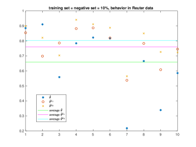
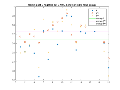
We applied our method on top 10 topics of single labeled documents in Reuters-21578 data[13], and 20 news group data[10]. we compare the result of traditional Naive Bayes estimator $\hat{\theta}_{i_{j}}$ and our estimator $\hat{\theta}_{i_{j}}^{L_{1}}$, $\hat{\theta}_{i_{j}}^{L_{2}}$, as well as $\hat{\theta}_{i_{j}}^{*}$. $t$ is chosen to be $2$ in all the following figures. The data in $S_{2}$ is generated randomly by not belong to a class, for example, if we know a document $d$ is in class $1$ among $10$ classes in Reuter’s data, to put $d$ in $S_{2}$, we randomly pick one class from $2$ to $10$, and mark $d$ not in that class. All Figures are put in the appendix.

First of all, we run all the algorithms on these two sample sets. We know that when sample size becomes large enough, three estimators actually convergence into the same thing, thus we take the training size relatively small. See Figure.1 and Figure.1. According from the experiment, we can see our methods are more accurate for most of the classes, and more accurate in average.

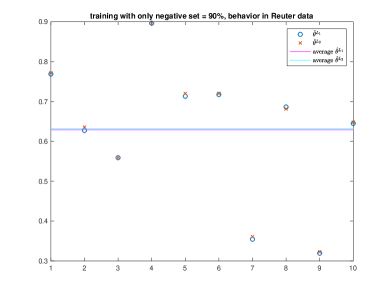
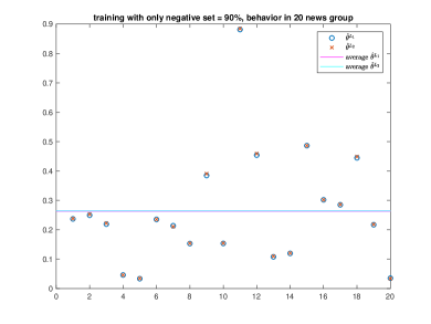
Then we consider a more extreme case. If we have a dataset with $|S_{1}|=0$, that is to say, we have no positive labeled data. In this setting, traditional Naive Bayes will not work, but what will we get from our estimators? See Figure.2 and Figure.2. We can see we can still get some information from negative labeled data. The accuracy is not as good as Figure.1 and Figure.1, that is because for each of the sample, negative label is only a part of information of positive label.

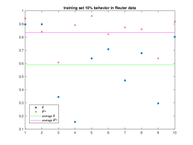
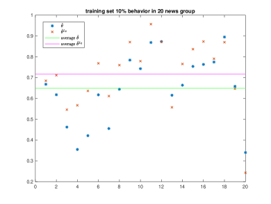
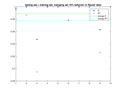
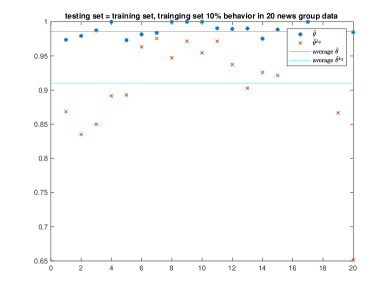
At last, we test our estimator $\hat{\theta}^{L_{2}}$ with only $S_{1}$ dataset, see Figure.3 and Figure.3. We can see our method achieve better result than traditional Naive Bayes estimator. We try to apply same training set and test the accuracy just on training set, we find traditional Naive Bayes estimator actually achieve better result, that means it might have more over-fitting problems, see Figure.4 and Figure.4.

6 Conclusion

We have presented an effective learning approach with a new labeling method for partially labeled document data, for some of which we only know the sample is surely not belonging to certain classes. We encode these labels as $y_{i}$ or $z_{i}$, and define maximum likelihood estimator $\hat{\theta}_{i_{j}}^{L_{1}}$, $\hat{\theta}_{i_{j}}^{L_{2}}$, as well as $\hat{\theta}_{i_{j}}^{*}$ for multinomial Naive Bayes model based on $L_{1}$ and $L_{2}$. There are several futher questions about these estimators:

1. We have proved that with multinomial Naive Bayes model, our estimators have smaller variance, which means our estimators can converge to true parameters with a faster rate than the standard Naive Bayes estimator.

   An interesting question is the following: if we consider a more general situation without the text classification background and the multinomial assumption, by solving the optimization problem (3.8) with $L_{1}$ and $L_{2}$, can we get the same conclusion with a more general chosen likelihood function $f_{i}$? If not, what assumption should we raise for $f_{i}$ to land on a similar conclusion?

2. The effectiveness of an algorithm in machine learning depends heavily upon well-labeled training samples; to some extent, our new estimator can utilize incorrect-labeled data or different-labeled data. Our estimator, especially $L_{2}$, can resolve this problem (3.2), since the incorrect-labeled data can be canceled out by the correct-labeled data, thus the partial-labeled data can still have its contribution.

   Another question is: besides $\hat{\theta}_{i_{j}}^{L_{1}}$ and $\hat{\theta}_{i_{j}}^{L_{2}}$, can we find other estimators, or even better estimators satisfying this property?

3. Based on our experiment, the traditional Naive Bayes estimator acts almost perfectly in the training set as well as during the cross validation stage, but the accuracy rate in the testing set is not ideal. To quantify this observation, we are still working on a valid justification that the traditional Naive Bayes estimator has a severe over-fitting problem in the training stage.

Appendix A Proof of Theorem 3.1

Proof A.1.

With assumption $\sum_{j=1}^{v}x_{j}=m$, we can rewrite (3.10) as:

$$\hat{\theta}_{i_{j}}=\frac{\sum_{d\in C_{i}}x_{j}}{\sum_{d\in C_{i}}m}=\frac{\sum_{d\in C_{i}}x_{j}}{|C_{i}|m}.$$

Since $d=(x_{1},x_{2},...,x_{v})$ is multinomial distribution, with $d$ in class $C_{i}$, we have: $E[x_{j}]=m\cdot\theta_{i_{j}}$, and $E[x_{j}^{2}]=m\theta_{i_{j}}(1-\theta_{i_{j}}+m\theta_{i_{j}}).$

1. $$\hat{\theta}_{i_{j}}=E[\frac{\sum_{d\in C_{i}}x_{j}}{|C_{i}|m}]=\frac{\sum_{d\in C_{i}}E[x_{j}]}{|C_{i}|m}=\frac{\sum_{d\in C_{i}}m\cdot\theta_{i_{j}}}{|C_{i}|m}=\theta_{i_{j}}.$$

   Thus $\hat{\theta}_{i_{j}}$ is unbiased.

2. By (1), we have:

   $$E[|\hat{\theta}_{i_{j}}-\theta_{i_{j}}|^{2}]=E[\hat{\theta}_{i_{j}}^{2}]-2\theta_{i_{j}}E[\hat{\theta}_{i_{j}}]+\theta_{i_{j}}^{2}=E[\hat{\theta}_{i_{j}}^{2}]-\theta_{i_{j}}^{2}.$$

   Then

   $$\hat{\theta}_{i_{j}}^{2}=\frac{(\sum_{d\in C_{i}}x_{j})^{2}}{|C_{i}|^{2}m^{2}}=\frac{\sum_{d\in C_{i}}x_{j}^{2}+\sum_{d_{1},d_{2}\in C_{i}}2x_{j}^{d_{1}}x_{j}^{d_{2}}}{|C_{i}|^{2}m^{2}},$$ (A.1)

   where $d_{i}=(x_{1}^{d_{i}},x_{2}^{d_{i}},...,x_{v}^{d_{i}})$ for $i=1,2$. Since:

   $$E[\sum_{d\in C_{i}}x_{j}^{2}]=\frac{|C_{i}|m\theta_{i_{j}}(1-\theta_{i_{j}}+m\theta_{i_{j}})}{|C_{i}|^{2}m^{2}}=\frac{\theta_{i_{j}}(1-\theta_{i_{j}}+m\theta_{i_{j}})}{|C_{i}|m},$$

   and

   $$E[\sum_{d_{1},d_{2}\in C_{i}}2x_{j}^{d_{1}}x_{j}^{d_{2}}]=\frac{|C_{i}|(|C_{i}|-1)m^{2}\theta_{i_{j}}^{2}}{|C_{i}|^{2}m^{2}}=\frac{(|C_{i}|-1)\theta_{i_{j}}^{2}}{|C_{i}|}.$$

   Plugging them into (A.1) obtains:

   $$E[\hat{\theta}_{i_{j}}^{2}]=\frac{\theta_{i_{j}}(1-\theta_{i_{j}})}{|C_{i}|m}+\theta_{i_{j}}^{2},$$

   thus: $E[|\hat{\theta}_{i_{j}}-\theta_{i_{j}}|^{2}]=\frac{\theta_{i_{j}}(1-\theta_{i_{j}})}{|C_{i}|m}$.

Appendix B Figures

Figure 1: We take 10 largest groups in Reuter-21578 dataset (a) and 20 news group dataset (b), and take 20% of the data as training set, among which $|S_{1}|=|S_{2}|$. The y-axis is the accuracy, and the x-axis is the class index.

Figure 2: We take 10 largest groups in Reuter-21578 dataset (a), and 20 news group dataset (b), and take 90% of the data as $S_{2}$ training set. The y-axis is the accuracy, and the x-axis is the class index.

Figure 3: We take 10 largest groups in Reuter-21578 dataset (a), and 20 news group dataset (b), and take 10% of the data as $S_{1}$ training set. The y-axis is the accuracy, and the x-axis is the class index.

Figure 4: We take 10 largest groups in Reuter-21578 dataset(a), and 20 news group dataset (b), and take 10% of the data as $S_{1}$ training set. We test the result on training set. The y-axis is the accuracy, and the x-axis is the class index.

References

• [1] Matthew R Boutell, Jiebo Luo, Xipeng Shen, and Christopher M Brown. Learning multi-label scene classification. Pattern recognition, 37(9):1757–1771, 2004.
• [2] Jiangning Chen, Heinrich Matzinger, Haoyan Zhai, and Mi Zhou. Centroid estimation based on symmetric kl divergence for multinomial text classification problem. arXiv preprint arXiv:1808.10261, 2018.
• [3] Corinna Cortes and Vladimir Vapnik. Support-vector networks. Machine learning, 20(3):273–297, 1995.
• [4] Timothee Cour, Ben Sapp, and Ben Taskar. Learning from partial labels. Journal of Machine Learning Research, 12(May):1501–1536, 2011.
• [5] Susan Dumais, John Platt, David Heckerman, and Mehran Sahami. Inductive learning algorithms and representations for text categorization. In Proceedings of the seventh international conference on Information and knowledge management, pages 148–155. ACM, 1998.
• [6] Nir Friedman, Dan Geiger, and Moises Goldszmidt. Bayesian network classifiers. Machine learning, 29(2-3):131–163, 1997.
• [7] Thomas Hofmann. Probabilistic latent semantic analysis. In Proceedings of the Fifteenth conference on Uncertainty in artificial intelligence, pages 289–296. Morgan Kaufmann Publishers Inc., 1999.
• [8] Rong Jin and Zoubin Ghahramani. Learning with multiple labels. In Advances in neural information processing systems, pages 921–928, 2003.
• [9] Thorsten Joachims. Text categorization with support vector machines: Learning with many relevant features. In European conference on machine learning, pages 137–142. Springer, 1998.
• [10] K. Lang. 20 newsgroups data set.
• [11] Pat Langley, Wayne Iba, Kevin Thompson, et al. An analysis of bayesian classifiers. In Aaai, volume 90, pages 223–228, 1992.
• [12] Leah S Larkey. Automatic essay grading using text categorization techniques. In Proceedings of the 21st annual international ACM SIGIR conference on Research and development in information retrieval, pages 90–95. ACM, 1998.
• [13] David D. Lewis. Reuters-21578.
• [14] Xiaoli Li and Bing Liu. Learning to classify texts using positive and unlabeled data. In IJCAI, volume 3, pages 587–592, 2003.
• [15] Pengfei Liu, Xipeng Qiu, and Xuanjing Huang. Recurrent neural network for text classification with multi-task learning. arXiv preprint arXiv:1605.05101, 2016.
• [16] Andrew McCallum. Multi-label text classification with a mixture model trained by em. In AAAI workshop on Text Learning, pages 1–7, 1999.
• [17] Nam Nguyen and Rich Caruana. Classification with partial labels. In Proceedings of the 14th ACM SIGKDD international conference on Knowledge discovery and data mining, pages 551–559. ACM, 2008.
• [18] S. Belongie P. Welinder, S. Branson and P. Perona. The multidimensional wisdom of crowds. In Advances in Neural Information Processing Systems, pages 2424–2432, 2010.
• [19] Juan Ramos et al. Using tf-idf to determine word relevance in document queries. In Proceedings of the first instructional conference on machine learning, volume 242, pages 133–142, 2003.
• [20] Irina Rish et al. An empirical study of the naive bayes classifier. In IJCAI 2001 workshop on empirical methods in artificial intelligence, volume 3, pages 41–46. IBM New York, 2001.
• [21] Karl-Michael Schneider. A new feature selection score for multinomial naive bayes text classification based on kl-divergence. In Proceedings of the ACL 2004 on Interactive poster and demonstration sessions, page 24. Association for Computational Linguistics, 2004.
• [22] Victor S Sheng, Foster Provost, and Panagiotis G Ipeirotis. Get another label? improving data quality and data mining using multiple, noisy labelers. In Proceedings of the 14th ACM SIGKDD international conference on Knowledge discovery and data mining, pages 614–622. ACM, 2008.
• [23] Duyu Tang, Bing Qin, and Ting Liu. Document modeling with gated recurrent neural network for sentiment classification. In Proceedings of the 2015 conference on empirical methods in natural language processing, pages 1422–1432, 2015.
• [24] Min-Ling Zhang, Bin-Bin Zhou, and Xu-Ying Liu. Partial label learning via feature-aware disambiguation. In Proceedings of the 22nd ACM SIGKDD International Conference on Knowledge Discovery and Data Mining, pages 1335–1344. ACM, 2016.
• [25] Min-Ling Zhang and Zhi-Hua Zhou. Ml-knn: A lazy learning approach to multi-label learning. Pattern recognition, 40(7):2038–2048, 2007.
• [26] Min-Ling Zhang and Zhi-Hua Zhou. A review on multi-label learning algorithms. IEEE transactions on knowledge and data engineering, 26(8):1819–1837, 2014.