The Implicit Metropolis-Hastings Algorithm

Abstract

Recent works propose using the discriminator of a GAN to filter out unrealistic samples of the generator. We generalize these ideas by introducing the implicit Metropolis-Hastings algorithm. For any implicit probabilistic model and a target distribution represented by a set of samples, implicit Metropolis-Hastings operates by learning a discriminator to estimate the density-ratio and then generating a chain of samples. Since the approximation of density ratio introduces an error on every step of the chain, it is crucial to analyze the stationary distribution of such chain. For that purpose, we present a theoretical result stating that the discriminator loss upper bounds the total variation distance between the target distribution and the stationary distribution. Finally, we validate the proposed algorithm both for independent and Markov proposals on CIFAR-10 and CelebA datasets.

1 Introduction

Learning a generative model from an empirical target distribution is one of the key tasks in unsupervised machine learning. Currently, Generative Adversarial Networks (GANs) (Goodfellow et al., 2014) are among the most successful approaches in building such models. Unlike conventional sampling techniques, such as Markov Chain Monte-Carlo (MCMC), they operate by learning the implicit probabilistic model, which allows for sampling but not for a density evaluation. Due to the availability of large amounts of empirical data, GANs find many applications in computer vision: image super-resolution (Ledig et al., 2017), image inpainting (Yu et al., 2018), and learning representations (Donahue et al., 2016).

Despite the practical success, GANs remain hard for theoretical analysis and do not provide any guarantees on the learned model. For now, most of the theoretical results assume optimality of the learned discriminator (critic) what never holds in practice (Goodfellow et al., 2014; Nowozin et al., 2016; Arjovsky et al., 2017). Moreover, there is empirical evidence that GANs do not learn to sample from a target distribution (Arora & Zhang, 2017).

Recently, the idea of a GAN postprocessing by filtering the generator was proposed in several works. Under the assumption that the learned discriminator evaluates the exact density-ratio they filter samples from a generator by rejection sampling (Azadi et al., 2018) or by the independent Metropolis-Hastings algorithm (Neklyudov et al., 2018; Turner et al., 2018). Since the assumption of the discriminator optimality never holds in practice, we still cannot be sure that the resulting distribution will be close to the target, we even cannot guarantee that we will improve the output of the generator.

In this work, we present a theoretical result that justifies the heuristic proposed by Neklyudov et al. (2018); Turner et al. (2018) and generalize the proposed algorithm to the case of any implicit probabilistic models — both independent and Markov. To do that, we consider some, maybe not optimal, discriminator in the Metropolis-Hastings test, and approach the problem from the MCMC perspective. Under reasonable assumptions, we derive an upper bound on the total variation distance between the target distribution and the stationary distribution of the produced chain, that can be minimized w.r.t. parameters of the discriminator.

On CIFAR-10 and CelebA datasets, we validate the proposed algorithm using different models as independent proposals: DCGAN (Radford et al., 2015) that is learned in terms of minimax game under a classical GAN approach; Wasserstein GAN with gradient penalty (Gulrajani et al., 2017) that minimizes Wasserstein distance estimated by the critic network; VAE (Kingma & Welling, 2014) that maximizes the evidence lower bound. For every proposal, we learn a discriminator from scratch and observe the monotonous improvement of metrics throughout the learning. Using the generator of WPGAN, we further improve its performance by traversing its latent space via a Markov chain and applying the proposed algorithm.

We summarize our main contributions as follows.

• We propose the implicit Metropolis-Hastings algorithm, that can be seen as an adaptation of the classical Metropolis-Hastings algorithm to the case of an implicit probabilistic model and an empirical target distribution (Section 3).

• We justify the algorithm proposed by Neklyudov et al. (2018) and Turner et al. (2018). In particular, we demonstrate that learning the discriminator via the binary cross-entropy minimizes an upper bound on the distance between the target distribution and the stationary distribution of the chain (Section 3.5).

• We empirically validate the obtained theoretical result on real-world datasets (CIFAR-10, CelebA) (Section 4.1). We also demonstrate empirical gains by applying our algorithm for Markov proposals (Section 4.2).

2 Background

2.1 The Metropolis-Hastings algorithm

The MH algorithm allows for sampling from an analytic target distribution $p(x)$ by filtering samples from a proposal distribution $q(x\,|\,y)$ that is also given in the analytic form. It operates by sampling a chain of correlated samples that converge in distribution to the target (see Algorithm 1).

Algorithm 1 The Metropolis-Hastings algorithm

0:  density of target distribution $\hat{p}(x)\propto p(x)$

0:  proposal distribution $q(x\,|\,y)$

  $y\leftarrow$ random init

  for $i=0\ldots n$ do

     sample proposal point $x\sim q(x\,|\,y)$

     $P=\min\{1,\frac{\hat{p}(x)q(y\,|\,x)}{\hat{p}(y)q(x\,|\,y)}\}$

     $x_{i}=\begin{cases}x,\text{ with probability }P\\ y,\text{ with probability }(1-P)\end{cases}$

     $y\leftarrow x_{i}$

  end for

   $\{x_{0},\ldots,x_{n}\}$

Algorithm 2 Metropolis-Hastings GAN

0:  target dataset $\mathcal{D}$

0:  learned generator $q(x)$, discriminator $d(\cdot)$

  $y\sim\mathcal{D}$ initialize from the dataset

  for $i=0\ldots n$ do

     sample proposal point $x\sim q(x)$

     $P=\min\{1,\frac{d(x)(1-d(y))}{(1-d(x))d(y)}\}$

     $x_{i}=\begin{cases}x,\text{ with probability }P\\ y,\text{ with probability }(1-P)\end{cases}$

     $y\leftarrow x_{i}$

  end for

   $\{x_{0},\ldots,x_{n}\}$

If we take a proposal distribution that is not conditioned on the previous point, we will obtain the independent MH algorithm. It operates in the same way, but samples all of the proposal points independently $q(x\,|\,y)=q(x)$.

2.2 Metropolis-Hastings GAN

Recent works (Neklyudov et al., 2018; Turner et al., 2018) propose to treat the generator of a GAN as an independent proposal distribution $q(x)$ and perform an approximate Metropolis-Hastings test via the discriminator. Authors motivate this approximation by the fact that the optimal discriminator evaluates the true density-ratio

$$d^{*}(x)=\frac{p(x)}{p(x)+q(x)}=\operatorname*{arg\,min}_{d}\bigg{[}-\mathbb{E}_{x\sim p(x)}\log d(x)-\mathbb{E}_{x\sim q(x)}\log(1-d(x))\bigg{]}.$$ (1)

Substituting the optimal discriminator in the acceptance test, one can obtain the Metropolis-Hastings correction of a GAN, that is described in Algorithm 2.

In contrast to the previous works, we take the non-optimality of the discriminator as given and analyze the stationary distribution of the resulting chain for both independent and Markov proposals. In Section 3, we formulate the implicit Metropolis-Hastings algorithm and derive an upper bound on the total variation distance between the target distribution and the stationary distribution of the chain. Then, in Appendix F, we justify Algorithm 2 by relating the obtained upper bound with the binary cross-entropy.

3 The Implicit Metropolis-Hastings Algorithm

Algorithm 3
The implicit Metropolis-Hastings algorithm

0:  target dataset $\mathcal{D}$

0:  implicit model $q(x\,|\,y)$

0:  learned discriminator $d(\cdot,\cdot)$

  $y\sim\mathcal{D}$ initialize from the dataset

  for $i=0\ldots n$ do

     sample proposal point $x\sim q(x\,|\,y)$

     $P=\min\{1,\frac{d(x,y)}{d(y,x)}\}$

     $x_{i}=\begin{cases}x,\text{ with probability }P\\ y,\text{ with probability }(1-P)\end{cases}$

     $y\leftarrow x_{i}$

  end for

   $\{x_{0},\ldots,x_{n}\}$

In this section, we describe the implicit Metropolis-Hastings algorithm and present a theoretical analysis of its stationary distribution.

The Implicit Metropolis-Hastings algorithm is aimed to sample from an empirical target distribution $p(x),\;x\in\mathbb{R}^{D}$, while being able to sample from an implicit proposal distribution $q(x\,|\,y)$. Given a discriminator $d(x,y)$, it generates a chain of samples as described in Algorithm 3.

We build our reasoning by first assuming that the chain is generated using some discriminator and then successively introducing conditions on the discriminator and upper bounding the distance between the chain and the target. Finally, we come up with an upper bound that can be minimized w.r.t. parameters of the discriminator. Here we consider the case of an implicit Markov proposal, but all of the derivations also hold for independent proposals.

The transition kernel of the implicit Metropolis-Hastings algorithm is

$$t(x\,|\,y)=q(x\,|\,y)\min\bigg{\{}1,\frac{d(x,y)}{d(y,x)}\bigg{\}}+\delta(x-y)\int dx^{\prime}q(x^{\prime}\,|\,y)\bigg{(}1-\min\bigg{\{}1,\frac{d(x^{\prime},y)}{d(y,x^{\prime})}\bigg{\}}\bigg{)}.$$ (2)

First of all, we need to ensure that the Markov chain defined by the transition kernel $t(x\,|\,y)$ converges to some stationary distribution $t_{\infty}(x)$. In order to do that, we require the proposal distribution $q(x\,|\,y)$ and the discriminator $d(x,y)$ to be continuous and positive on $\mathbb{R}^{D}\times\mathbb{R}^{D}$. In Appendix A, we show that these requirements guarantee the following properties of the transition kernel $t$:

• the kernel $t$ defines a correct conditional distribution;

• the Markov chain defined by $t$ is irreducible;

• the Markov chain defined by $t$ is aperiodic.

These properties imply convergence of the Markov chain defined by $t$ to some stationary distribution $t_{\infty}$ (Roberts et al., 2004).

Further, we want the stationary distribution $t_{\infty}$ of our Markov chain to be as close as possible to the target distribution $p$. To measure the closeness of distributions, we consider a standard metric for analysis in MCMC — the total variation distance

$$\left\lVert t_{\infty}-p\right\rVert_{TV}=\frac{1}{2}\int|t_{\infty}(x)-p(x)|dx.$$ (3)

We assume the proposal $q(x\,|\,y)$ to be given, but different $d(x,y)$ may lead to different $t_{\infty}$. That is why we want to derive an upper bound on the distance $\left\lVert t_{\infty}-p\right\rVert_{TV}$ and minimize it w.r.t. parameters of the discriminator $d(x,y)$. We derive this upper bound in three steps in the following subsections.

3.1 Fast convergence

In practice, estimation of the stationary distribution $t_{\infty}$ by running a chain is impossible. Nevertheless, if we know that the chain converges fast enough, we can upper bound the distance $\left\lVert t_{\infty}-p\right\rVert_{TV}$ using the distance $\left\lVert t_{1}-p\right\rVert_{TV}$, where $t_{1}$ is the one-step distribution $t_{1}(x)=\int t(x\,|\,y)t_{0}(y)dy$, and $t_{0}$ is some initial distribution of the chain.

To guarantee fast convergence of a chain, we propose to use the minorization condition (Roberts et al., 2004). For a transition kernel $t(x\,|\,y)$, it requires that exists such $\varepsilon>0$ and a distribution $\nu$ that the following condition is satisfied

$$t(x\,|\,y)>\varepsilon\nu(x)\;\;\forall(x,y)\in\mathbb{R}^{D}\times\mathbb{R}^{D}.$$ (4)

When a transition kernel satisfies the minorization condition, the Markov chain converges "fast" to the stationary distribution. We formalize this statement in the following Proposition.

Proposition 1

Consider a transition kernel $t(x\,|\,y)$ that satisfies the minorization condition $t(x\,|\,y)>\varepsilon\nu(x)$ for some $\varepsilon>0$, and distribution $\nu$. Then the distance between two consequent steps decreases as:

$$\left\lVert t_{n+2}-t_{n+1}\right\rVert_{TV}\leq(1-\varepsilon)\left\lVert t_{n+1}-t_{n}\right\rVert_{TV},$$ (5)

where distribution $t_{k+1}(x)=\int t(x\,|\,y)t_{k}(y)dy$.

This result could be considered as a corollary of Theorem 8 in Roberts et al. (2004). For consistency, we provide an independent proof of Proposition 1 in Appendix B.

To guarantee minorization condition of our transition kernel $t(x\,|\,y)$, we require the proposal $q(x\,|\,y)$ to satisfy minorization condition with some constant $\varepsilon$ and distribution $\nu$ (note that for an independent proposal, the minorization condition holds automatically with $\varepsilon=1$). Also, we limit the range of the discriminator as $d(x,y)\in[b,1]\;\forall x,y$, where $b$ is some positive constant that can be treated as a hyperparameter of the algorithm. These requirements imply

$$t(x\,|\,y)\geq bq(x\,|\,y)>b\varepsilon\nu(x).$$ (6)

Using Proposition 1 and minorization condition (6) for $t$, we can upper bound the TV-distance between an initial distribution $t_{0}$ and the stationary distribution $t_{\infty}$ of implicit Metropolis-Hastings.

$$\left\lVert t_{\infty}-t_{0}\right\rVert_{TV}\leq\sum_{i=0}^{\infty}\left\lVert t_{i+1}-t_{i}\right\rVert_{TV}\leq\sum_{i=0}^{\infty}(1-b\varepsilon)^{i}\left\lVert t_{1}-t_{0}\right\rVert_{TV}=\frac{1}{b\varepsilon}\left\lVert t_{1}-t_{0}\right\rVert_{TV}$$ (7)

Taking the target distribution $p(x)$ as the initial distribution $t_{0}(x)$ of our chain $t(x\,|\,y)$, we reduce the problem of estimation of the distance $\left\lVert t_{\infty}-p\right\rVert_{TV}$ to the problem of estimation of the distance $\left\lVert t_{1}-p\right\rVert_{TV}$:

$$\left\lVert t_{\infty}-p\right\rVert_{TV}\leq\frac{1}{b\varepsilon}\left\lVert t_{1}-p\right\rVert_{TV}=\frac{1}{b\varepsilon}\cdot\frac{1}{2}\int dx\bigg{|}\int t(x\,|\,y)p(y)dy-p(x)\bigg{|}.$$ (8)

However, the estimation of this distance raises two issues. Firstly, we need to get rid of the inner integral $\int t(x\,|\,y)p(y)dy$. Secondly, we need to bypass the evaluation of densities $t(x\,|\,y)$ and $p(x)$. We address these issues in the following subsections.

3.2 Dealing with the integral inside of the nonlinearity

For now, assume that we have access to the densities $t(x\,|\,y)$ and $p(x)$. However, evaluation of the density $t_{1}(x)$ is an infeasible problem in most cases. To estimate $t_{1}(x)$, one would like to resort to the Monte-Carlo estimation:

$$t_{1}(x)=\int t(x\,|\,y)p(y)dy=\mathbb{E}_{y\sim p(y)}t(x\,|\,y).$$ (9)

However, straightforward estimation of $t_{1}(x)$ results in a biased estimation of $\left\lVert t_{1}-p\right\rVert_{TV}$, since the expectation is inside of a nonlinear function. To overcome this problem, we upper bound this distance in the following proposition.

Proposition 2

For the kernel $t(x\,|\,y)$ of the implicit Metropolis-Hastings algorithm, the distance between initial distribution $p(x)$ and the distribution $t_{1}(x)$ has the following upper bound

$$\left\lVert t_{1}-p\right\rVert_{TV}\leq 2\left\lVert q(y\,|\,x)p(x)-q(x\,|\,y)p(y)\frac{d(x,y)}{d(y,x)}\right\rVert_{TV},$$ (10)

where the TV-distance on the right side is evaluated in the joint space $(x,y)\in\mathbb{R}^{D}\times\mathbb{R}^{D}$.

For the proof of this proposition, see Appendix C. Note that the obtained upper bound no longer requires evaluation of an integral inside of a nonlinear function. Moreover, the right side of (10) has a reasonable motivation since it is an averaged $l_{1}$ error of the density ratio estimation.

$$\left\lVert q(y\,|\,x)p(x)-q(x\,|\,y)p(y)\frac{d(x,y)}{d(y,x)}\right\rVert_{TV}=\frac{1}{2}\int p(y)q(x\,|\,y)\bigg{|}\frac{q(y\,|\,x)p(x)}{q(x\,|\,y)p(y)}-\frac{d(x,y)}{d(y,x)}\bigg{|}dxdy$$ (11)

In this formulation, we see that we still could achieve zero value of $\left\lVert t_{1}-p\right\rVert_{TV}$ if we could take such discriminator that estimates the desired density ratio $\frac{d(x,y)}{d(y,x)}=\frac{q(y\,|\,x)p(x)}{q(x\,|\,y)p(y)}$.

3.3 Dealing with the evaluation of densities

For an estimation of the right side of (10), we still need densities $p(x)$ and $q(x\,|\,y)$. To overcome this issue, we propose to upper bound the obtained TV distance via KL-divergence. Then we show that obtained KL divergence decomposes into two terms: the first term requires evaluation of densities but does not depend on the discriminator $d(x,y)$, and the second term can be estimated only by evaluation of $d(x,y)$ on samples from $p(x)$ and $q(x\,|\,y)$.

To upper bound the TV-distance $\left\lVert\alpha-\beta\right\rVert_{TV}$ via KL-divergence $\mathrm{KL}(\alpha\|\beta)$ one can use well-known Pinsker’s inequality:

$$2\left\lVert\alpha-\beta\right\rVert_{TV}^{2}\leq\mathrm{KL}(\alpha\|\beta).$$ (12)

However, Pinsker’s inequality assumes that both $\alpha$ and $\beta$ are distributions, while it is not always true for function $q(x\,|\,y)p(y)\frac{d(x,y)}{d(y,x)}$ in (10). In the following proposition, we extend Pinsker’s inequality to the case when one of the functions is not normalized.

Proposition 3

For a distribution $\alpha(x)$ and some positive function $f(x)>0\;\forall x$ the following inequality holds:

$$\left\lVert\alpha-f\right\rVert_{TV}^{2}\leq\bigg{(}\frac{2C_{f}+1}{6}\bigg{)}(\widehat{\mathrm{KL}}(\alpha\|f)+C_{f}-1),$$ (13)

where $C_{f}$ is the normalization constant of function $f$: $C_{f}=\int f(x)dx$, and $\widehat{\mathrm{KL}}(\alpha\|f)$ is the formal evaluation of the KL divergence

$$\widehat{\mathrm{KL}}(\alpha\|f)=\int\alpha(x)\log\frac{\alpha(x)}{f(x)}dx.$$ (14)

The proof of the proposition is in Appendix D.

Now we use this proposition to upper bound the right side of (10):

$$\left\lVert q(y\,|\,x)p(x)-q(x\,|\,y)p(y)\frac{d(x,y)}{d(y,x)}\right\rVert_{TV}^{2}\leq$$ (15)

$$\leq\bigg{(}\frac{2C+1}{6}\bigg{)}\bigg{(}\widehat{\mathrm{KL}}\bigg{(}q(y\,|\,x)p(x)\bigg{\|}q(x\,|\,y)p(y)\frac{d(x,y)}{d(y,x)}\bigg{)}+C-1\bigg{)}.$$

Here $C$ is the normalization constant of $q(x\,|\,y)p(y)\frac{d(x,y)}{d(y,x)}$. For the multiplicative term $(2C+1)/6$, we upper bound $C$ as

$$C=\int q(x\,|\,y)p(y)\frac{d(x,y)}{d(y,x)}dxdy\leq\int q(x\,|\,y)p(y)\frac{1}{b}dxdy=\frac{1}{b},$$ (16)

since we limit the range of the discriminator as $d(x,y)\in[b,1]\;\;\forall x,y$.

Summing up the results (8), (10), (15), (16), we obtain the final upper bound as follows.

$$\left\lVert t_{\infty}-p\right\rVert_{TV}^{2}\leq\frac{1}{b^{2}\varepsilon^{2}}\left\lVert t_{1}-p\right\rVert_{TV}^{2}\leq\frac{4}{b^{2}\varepsilon^{2}}\left\lVert q(y\,|\,x)p(x)-q(x\,|\,y)p(y)\frac{d(x,y)}{d(y,x)}\right\rVert_{TV}^{2}\leq$$ (17)

$$\leq\bigg{(}\frac{4+2b}{3\varepsilon^{2}b^{3}}\bigg{)}\bigg{(}\underbrace{\text{\Large$\mathbb{E}$}_{\text{\footnotesize$\begin{matrix}x\sim p(x)\\ y\sim q(y\,|\,x)\end{matrix}$}}\bigg{[}\log\frac{d(y,x)}{d(x,y)}+\frac{d(y,x)}{d(x,y)}\bigg{]}}_{\text{loss for the discriminator}}-1+\mathrm{KL}\bigg{(}q(y\,|\,x)p(x)\bigg{\|}q(x\,|\,y)p(y)\bigg{)}\bigg{)}$$

Minimization of the resulting upper bound w.r.t. the discriminator $d(x,y)$ is equivalent to the following optimization problem:

$$\min_{d}\text{\Large$\mathbb{E}$}_{\text{\footnotesize$\begin{matrix}x\sim p(x)\\ y\sim q(y\,|\,x)\end{matrix}$}}\bigg{[}\log\frac{d(y,x)}{d(x,y)}+\frac{d(y,x)}{d(x,y)}\bigg{]}.$$ (18)

Thus, we derive the loss function that we can unbiasedly estimate and minimize w.r.t. parameters of $d(x,y)$. We analyze the optimal solution in the following subsection.

3.4 The optimal discriminator

By taking the derivative of objective (18), we show (see Appendix E) that the optimal discriminator $d^{*}$ must satisfy

$$\frac{d^{*}(x,y)}{d^{*}(y,x)}=\frac{q(y\,|\,x)p(x)}{q(x\,|\,y)p(y)}.$$ (19)

When the loss function (18) achieves its minimum, it becomes

$$\text{\Large$\mathbb{E}$}_{\text{\footnotesize$\begin{matrix}x\sim p(x)\\ y\sim q(y\,|\,x)\end{matrix}$}}\bigg{[}\log\frac{q(x\,|\,y)p(y)}{q(y\,|\,x)p(x)}+\frac{q(x\,|\,y)p(y)}{q(y\,|\,x)p(x)}\bigg{]}=-\mathrm{KL}\bigg{(}q(y\,|\,x)p(x)\bigg{\|}q(x\,|\,y)p(y)\bigg{)}+1$$ (20)

Substituting this equation into (17), we achieve $\left\lVert t_{\infty}-p\right\rVert_{TV}=0$. However, since we limit the range of the discriminator $d(x,y)\in[b,1]$, the optimal solution could be achieved only when the density-ratio lies in the following range:

$$\forall x,y\;\;\;\;\frac{q(y\,|\,x)p(x)}{q(x\,|\,y)p(y)}\in[b,b^{-1}].$$ (21)

Therefore, $b$ should be chosen small enough that range $[b,b^{-1}]$ includes all the possible values of density-ratio. Such $b>0$ exists if the support of the target distribution is compact. Indeed, if we have positive $p(x)$ and $q(x\,|\,y)$ on compact support, we can find a minimum of the density-ratio and set $b$ to that minimum. Moreover, taking a positive $q(x\,|\,y)$ on a compact support yields minorization condition for the $q(x\,|\,y)$.

If the support of target distribution is not compact, we may resort to the approximation of the target distribution on some smaller compact support that contains say $99.9\%$ of the whole mass of target distribution. In practice, many problems of generative modeling are defined on compact support, e.g. the distribution of images lies in finite support since we represent an image by pixels values.

3.5 Relation to the cross-entropy

It is possible to upper bound the loss (18) by the binary cross-entropy. For a Markov proposal, it is

$$\text{\Large$\mathbb{E}$}_{\text{\footnotesize$\begin{matrix}x\sim p(x)\\ y\sim q(y\,|\,x)\end{matrix}$}}\bigg{[}\log\frac{d(y,x)}{d(x,y)}+\frac{d(y,x)}{d(x,y)}\bigg{]}\leq\text{\Large$\mathbb{E}$}_{\text{\footnotesize$\begin{matrix}x\sim p(x)\\ y\sim q(y\,|\,x)\end{matrix}$}}\bigg{[}-\log d(x,y)-\log(1-d(y,x))+\frac{1}{b}\bigg{]}.$$ (22)

In the case of an independent proposal, we factorize the discriminator as $d(x,y)=d(x)(1-d(y))$ and obtain the following inequality (see Appendix F).

$$\text{\Large$\mathbb{E}$}_{\text{\footnotesize$\begin{matrix}x\sim p(x)\\ y\sim q(y\,|\,x)\end{matrix}$}}\bigg{[}\log\frac{d(y,x)}{d(x,y)}+\frac{d(y,x)}{d(x,y)}\bigg{]}\leq-\mathbb{E}_{x\sim p(x)}\log d(x)-\mathbb{E}_{y\sim q(y)}\log(1-d(y))+\frac{1}{b}$$ (23)

Thus, learning a discriminator via the binary cross-entropy, we also minimize the distance $\left\lVert t_{\infty}-p\right\rVert_{TV}$. This fact justifies Algorithm 2.

Table 1: Different losses for a density-ratio estimation.

Probosal	Name	Loss
Markov	Upper bound (UB)	$\displaystyle\int dxdy~{}p(x)q(y\,|\,x)\bigg{[}\log\frac{d(y,x)}{d(x,y)}+\frac{d(y,x)}{d(x,y)}\bigg{]}$
	Markov cross-entropy (MCE)	$\displaystyle\int dxdy~{}p(x)q(y\,|\,x)[-\log d(x,y)-\log(1-d(y,x))]$
Independent	Conventional cross-entropy (CCE)	$\displaystyle\int dxdy~{}p(x)q(y)[-\log d(x)(1-d(y))]$

4 Experiments

We present an empirical evaluation of the proposed algorithm and theory for both independent and Markov proposals. In both cases sampling via the implicit MH algorithm is better than the straightforward sampling from a generator. For independent proposals, we validate our theoretical result by demonstrating monotonous improvements of the sampling procedure throughout the learning of the discriminator. Further, the implicit MH algorithm with a Markov proposal compares favorably against Algorithm 2 proposed by (Neklyudov et al., 2018; Turner et al., 2018). Code reproducing all experiments is available online.

Since one can evaluate the total variation distance only when explicit densities are given, we show its monotonous fall only for a synthetic example (Appendix G). For complex empirical distributions, we consider the problem of sampling from the space of images (CIFAR-10 and CelebA datasets) and resort to the conventional metrics for the performance evaluation: the Inception Score (IS) (Salimans et al., 2016) and Frechet Inception Distance (FID) (Heusel et al., 2017). Note that these metrics rely heavily on the implementation of Inception network (Barratt & Sharma, 2018); therefore, for all experiments, we use PyTorch version of the Inception V3 network (Paszke et al., 2017).

4.1 Independent proposals

Since we propose to use the implicit MH algorithm for any implicit sampler, we consider three models that are learned under completely different approaches: Wasserstein GAN with gradient penalty (WPGAN) (Gulrajani et al., 2017), Deep Convolutional GAN (DCGAN) (Radford et al., 2015), Variational Auto-Encoder (VAE) (Kingma & Welling, 2014). To run the MH algorithm, we treat these models as independent proposals and learn the discriminator for acceptance test from scratch.

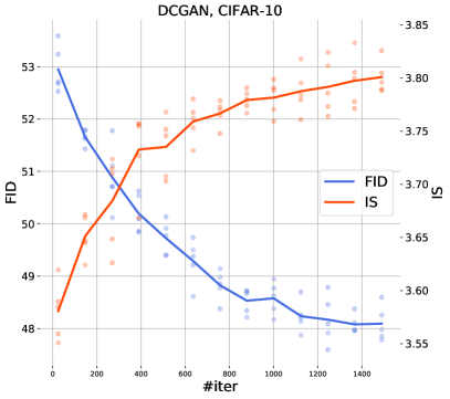
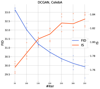
Figure 6: Monotonous improvements in terms of FID and IS for the learning of discriminator by CCE. During iterations, we evaluate metrics $5$ times (scatter) and then average them (solid lines). For a single metric evaluation, we use 10k samples. Higher values of IS and lower values of FID are better. Performance for the original generator corresponds to $0$th iteration of a discriminator.

Our theoretical result says that the total variation distance between the stationary distribution and the target can be upper bounded by different losses (see Table 1). Note, that we also can learn a discriminator by UB and MCE for independent proposals; however, in practice, we found that CCE performs slightly better. In Figure 6, we demonstrate that the minimization of CCE leads to better IS and FID throughout the learning of a discriminator (see plots for DCGAN in Appendix H).

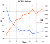
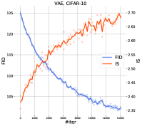
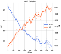
Figure 1: Monotonous improvements in terms of FID and IS for the learning of discriminator by CCE. During iterations, we evaluate metrics $5$ times (scatter) and then average them (solid lines). For a single metric evaluation, we use 10k samples. Higher values of IS and lower values of FID are better. Performance for the original generator corresponds to $0$th iteration of a discriminator.

4.2 Markov proposals

To simulate Markov proposals we take the same WPGAN as in the independent case and traverse its latent space by a Markov chain. Taking the latent vector $z_{y}$ for the previous image $y$, we sample the next vector $z_{x}$ via HMC and obtain the next image $x=g(z_{x})$ by the generator $g(\cdot)$, thus simulating a Markov proposal $q(x\,|\,y)$. Sampling via HMC from the Gaussian is equivalent to the interpolation between the previous accepted point $z_{y}$ and the random vector $v$:

$$z_{x}=\cos(t)z_{y}+\sin(t)v,\;\;\;v\sim\mathcal{N}(0,I).$$ (24)

In our experiments, we take $t=\pi/3$. For loss estimation, we condition samples from the proposal on samples from the dataset $x\sim q(x\,|\,y),y\sim p(y)$. However, to sample an image $x\sim q(x\,|\,y)$ we need to know the latent vector $z_{y}$ for an image $y$ from the dataset. We find such vectors by optimization in the latent space, minimizing the $l_{2}$ reconstruction error (reconstructions are in Fig. 2).

To filter a Markov proposal, we need to learn a pairwise discriminator, as suggested in Section 3. For this purpose, we take the same architecture of the discriminator as in the independent case and put the difference of its logits $\text{net}(\cdot)$ into the sigmoid.

$$d(x,y)=\frac{1}{1+\exp(\text{net}(y)-\text{net}(x))}$$ (25)

Then we learn this discriminator by minimization of UB and MCE (see Table 1).

In Figure 3, we demonstrate that our Markov proposal compares favorably not only against the original generator of WPGAN, but also against the chain obtained by the independent sampler (Algorithm 2). To provide the comparison, we evaluate both the performance (IS, FID) and computational efforts (rejection rate), showing that for the same rejection rate, our method results in better metrics.

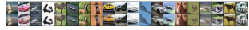
Figure 2: Samples from CIFAR-10 (top line) and their reconstructions (bottom line)

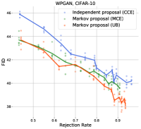
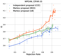
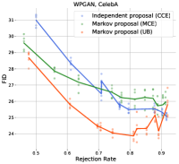
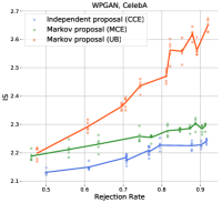
Figure 3: Comparison between different discriminators for the same generator of WPGAN in terms of performance (IS, FID) and computational efforts (rejection rate). Higher values of IS and lower values of FID are better. For a single metric evaluation, we use 10k samples. For every snapshot of a discriminator, we evaluate metrics $5$ times (scatter) and then average them (solid lines).

5 Conclusion

In this paper, we propose the implicit Metropolis-Hastings algorithm for sampling from an empirical target distribution using an implicit probabilistic model as the proposal. In the theoretical part of the paper, we upper bound the distance between the target distribution and the stationary distribution of the chain. The contribution of the derived upper bound is two-fold. We justify the heuristic algorithm proposed by (Neklyudov et al., 2018; Turner et al., 2018) and derive the loss functions for the case of Markov proposal. Moreover, the post-processing with the implicit Metropolis-Hastings algorithm can be seen as a justification or enhancement of any implicit model. In the experimental part of the paper, we empirically validate the proposed algorithm on the real-world datasets (CIFAR-10 and CelebA). For both tasks filtering with the proposed algorithm alleviates the gap between target and proposal distributions.

Appendix A The existence of stationary distribution for the transition kernel of IMH

Let us recall that transition kernel of the implicit Metropolis-Hastings algorithm is defined as

$$t(x\,|\,y)=q(x\,|\,y)\min\bigg{\{}1,\frac{d(x,y)}{d(y,x)}\bigg{\}}+\delta(x-y)\int dx^{\prime}q(x^{\prime}\,|\,y)\bigg{(}1-\min\bigg{\{}1,\frac{d(x^{\prime},y)}{d(y,x^{\prime})}\bigg{\}}\bigg{)}.$$ (26)

In this section we show that such kernel converges to some stationary distribution if the proposal distribution $q(x\,|\,y)$ and the function $d(x,y)$ are continuous and positive on $\mathbb{R}^{D}\times\mathbb{R}^{D}$.

Firstly, we validate that such transition kernel defines a correct conditional distribution.

$$t(x\,|\,y)\geq q(x\,|\,y)\min\bigg{\{}1,\frac{d(x,y)}{d(y,x)}\bigg{\}}>0\;\;\forall x,y\;\implies\;t_{1}(x)=\int t(x\,|\,y)t_{0}(y)dy>0\;\;\forall x$$ (27)

Normalization constant of $t_{1}$ can be obtained by straightforward evaluation of the integral:

$$t_{1}(x)= \int dyq(x\,|\,y)t_{0}(y)\min\bigg{\{}1,\frac{d(x,y)}{d(y,x)}\bigg{\}}+$$ (28)

$$+\int dy\delta(x-y)t_{0}(y)\int dx^{\prime}q(x^{\prime}\,|\,y)\bigg{(}1-\min\bigg{\{}1,\frac{d(x^{\prime},y)}{d(y,x^{\prime})}\bigg{\}}\bigg{)}$$ (29)

$$t_{1}(x)= \int dyq(x\,|\,y)t_{0}(y)\min\bigg{\{}1,\frac{d(x,y)}{d(y,x)}\bigg{\}}+t_{0}(x)-$$ (30)

$$-\int dx^{\prime}q(x^{\prime}\,|\,x)t_{0}(x)\min\bigg{\{}1,\frac{d(x^{\prime},x)}{d(x,x^{\prime})}\bigg{\}}$$ (31)

$$\int t_{1}(x)dx= \int dxdyq(x\,|\,y)t_{0}(y)\min\bigg{\{}1,\frac{d(x,y)}{d(y,x)}\bigg{\}}+\int t_{0}(x)dx-$$ (32)

$$-\int dxdx^{\prime}q(x^{\prime}\,|\,x)t_{0}(x)\min\bigg{\{}1,\frac{d(x^{\prime},x)}{d(x,x^{\prime})}\bigg{\}}$$ (33)

$$\int t_{1}(x)dx= \int t_{0}(x)dx=1$$ (34)

A.1 Irreducibility

Irreducibility of the chain can be straightforwardly proven by adaptation of the proof from (Roberts et al., 2004).

Consider some set $A$ such that $p(A)>0$. Then there exist $R>0$ such that $p(A_{R})>0$ where $A_{R}=A\cap B_{R}(0)$ and $B_{R}(0)$ is a ball with radius $R$ centered at zero. For continuous and positive $d(x,y)$ and $q(x\,|\,y)$ on $\mathbb{R}^{D}\times\mathbb{R}^{D}$ there exist $\varepsilon>0$ such that

$$\inf_{x,y\in A_{R}}q(x\,|\,y)\min\bigg{\{}1,\frac{d(x,y)}{d(y,x)}\bigg{\}}\geq\inf_{x,y\in B_{R}}q(x\,|\,y)\min\bigg{\{}1,\frac{d(x,y)}{d(y,x)}\bigg{\}}\geq\varepsilon.$$ (35)

Hence

$$t(A\,|\,y)\geq t(A_{R}\,|\,y)\geq\int_{A_{R}}q(x\,|\,y)\min\bigg{\{}1,\frac{d(x,y)}{d(y,x)}\bigg{\}}dx\geq\varepsilon|A_{R}|>0.$$ (36)

Thus the chain defined by $t(x\,|\,y)$ is irreducible.

A.2 Aperiodicity

Aperiodicity of the chain can be straightforwardly proven by adaptation of the proof from (Roberts et al., 2004).

Assume there exist two disjoint sets $A_{1}$ and $A_{2}$, such that for any starting point $y\in A_{1}$ the transition $t(x\,|\,y)$ ends in $A_{2}$, i.e. $t(A_{2}\,|\,y)=1$. However, by positivity of $d(x,y)$ and $q(x\,|\,y)$ we have

$$t(A_{1}\,|\,y)=\int_{A_{1}}q(x\,|\,y)\min\bigg{\{}1,\frac{d(x,y)}{d(y,x)}\bigg{\}}dx>0\implies t(A_{2}\,|\,y)<1.$$ (37)

Appendix B Proof of Proposition 1

We consider some ergodic chain with kernel $t(x\,|\,y)$ and assume that $t(x\,|\,y)$ satisfy minorization condition, i.e. for some distribution $\nu$ and some $\varepsilon>0$ the following inequality holds:

$$t(x\,|\,y)\geq\varepsilon\nu(x),\;\;\forall x,y.$$ (38)

We denote a distribution after $n$ steps of $t(x\,|\,y)$ as $t_{n}(x\,|\,y)$. Such distribution is defined by the recurrent formula:

$$t_{n+1}(x)=\int t(x\,|\,y)t_{n-1}(y)dy.$$ (39)

Denoting the difference between two consequent distributions as $\Delta_{n}$, we study how the operator $t(x\,|\,y)$ changes the $l_{1}$-norm of $\Delta_{n}$.

$$t_{n+1}(y)=t_{n}(y)+\Delta_{n}(y)\implies\int t(x\,|\,y)t_{n+1}(y)dy=\int t(x\,|\,y)t_{n}(y)dy+\int t(x\,|\,y)\Delta_{n}(y)dy$$ (40)

Therefore

$$\left\lVert t_{n+1}-t_{n}\right\rVert_{TV}=\frac{1}{2}\int|\Delta_{n}(y)|dy,\;\;\text{and}\;\;\left\lVert t_{n+2}-t_{n+1}\right\rVert_{TV}=\frac{1}{2}\int\bigg{|}\int t(x\,|\,y)\Delta_{n}(y)dy\bigg{|}dx.$$ (41)

Note that $\Delta_{n}$ integrates in zero

$$\int\Delta_{n}(y)dy=\int t_{n+1}(y)dy-\int t_{n}(y)dy=0.$$ (42)

Using that fact we can rewrite the following integral

$$\int t(x\,|\,y)\Delta_{n}(y)dy=\int(t(x\,|\,y)-\varepsilon\nu(x))\Delta_{n}(y)dy$$ (43)

$$\frac{1}{2}\int\bigg{|} \int t(x\,|\,y)\Delta_{n}(y)dy\bigg{|}dx\leq\frac{1}{2}\int(t(x\,|\,y)-\varepsilon\nu(x))|\Delta_{n}(y)|dydx=(1-\varepsilon)\frac{1}{2}\int|\Delta_{n}(y)|dy$$ (44)

Using the last inequality and equalities from (41), we obtain

$$\left\lVert t_{n+2}-t_{n+1}\right\rVert_{TV}\leq(1-\varepsilon)\left\lVert t_{n+1}-t_{n}\right\rVert_{TV}.$$ (45)

Appendix C Proof of Proposition 2

For the kernel of implicit Metropolis-Hastings algorithm:

$$t(x\,|\,y)=q(x\,|\,y)\min\bigg{\{}1,\frac{d(x,y)}{d(y,x)}\bigg{\}}+\delta(x-y)\int dx^{\prime}q(x^{\prime}\,|\,y)\bigg{(}1-\min\bigg{\{}1,\frac{d(x^{\prime},y)}{d(y,x^{\prime})}\bigg{\}}\bigg{)},$$ (46)

we want to derive upper bound on the length of the first step in terms of TV-distance

$$\left\lVert t_{1}-p\right\rVert_{TV}=\frac{1}{2}\int dx\bigg{|}\int dyt(x\,|\,y)p(y)-p(x)\bigg{|}.$$ (47)

Firstly, we take the integral inside of TV-distance:

$$\int dyt(x\,|\,y)p(y)= \int dyq(x\,|\,y)p(y)\min\bigg{\{}1,\frac{d(x,y)}{d(y,x)}\bigg{\}}+\int dy\delta(x-y)p(y)-$$ (48)

$$-\int dx^{\prime}dy\delta(x-y)q(x^{\prime}\,|\,y)p(y)\min\bigg{\{}1,\frac{d(x^{\prime},y)}{d(y,x^{\prime})}\bigg{\}}=$$ (49)

$$=\int dyq(x\,|\,y)p(y) \min\bigg{\{}1,\frac{d(x,y)}{d(y,x)}\bigg{\}}+p(x)-\int dx^{\prime}q(x^{\prime}\,|\,x)p(x)\min\bigg{\{}1,\frac{d(x^{\prime},x)}{d(x,x^{\prime})}\bigg{\}}=$$ (50)

$$=\int dyq(x\,|\,y)p(y) \min\bigg{\{}1,\frac{d(x,y)}{d(y,x)}\bigg{\}}+p(x)-\int dyq(y\,|\,x)p(x)\min\bigg{\{}1,\frac{d(y,x)}{d(x,y)}\bigg{\}}$$ (51)

Substituting this formula into (47) we obtain

$$\left\lVert t_{1}-p\right\rVert_{TV}= \frac{1}{2}\int dx\bigg{|}\int dyq(x\,|\,y)p(y)\min\bigg{\{}1,\frac{d(x,y)}{d(y,x)}\bigg{\}}-\int dyq(y\,|\,x)p(x)\min\bigg{\{}1,\frac{d(y,x)}{d(x,y)}\bigg{\}}\bigg{|}\leq$$ (52)

$$\leq \frac{1}{2}\int dxdy\bigg{|}q(x\,|\,y)p(y)\min\bigg{\{}1,\frac{d(x,y)}{d(y,x)}\bigg{\}}-q(y\,|\,x)p(x)\min\bigg{\{}1,\frac{d(y,x)}{d(x,y)}\bigg{\}}\bigg{|}=$$ (53)

Note that changing variables in integral does not change value of function, hence we can integrate over the half of the space and then multiply the integral by $2$:

$$= \int_{A}dxdy\bigg{|}q(x\,|\,y)p(y)\min\bigg{\{}1,\frac{d(x,y)}{d(y,x)}\bigg{\}}-q(y\,|\,x)p(x)\min\bigg{\{}1,\frac{d(y,x)}{d(x,y)}\bigg{\}}\bigg{|}=$$ (54)

$$A=\bigg{\{}x,y:\frac{d(x,y)}{d(y,x)}\geq 1\bigg{\}}$$ (55)

$$= \int_{A}dxdy\bigg{|}q(x\,|\,y)p(y)-q(y\,|\,x)p(x)\min\bigg{\{}1,\frac{d(y,x)}{d(x,y)}\bigg{\}}\bigg{|}$$ (56)

Thus, we obtain

$$\left\lVert t_{1}-p\right\rVert_{TV}\leq 2\left\lVert q(x\,|\,y)p(y)-q(y\,|\,x)p(x)\min\bigg{\{}1,\frac{d(y,x)}{d(x,y)}\bigg{\}}\right\rVert_{TV}$$ (57)

Appendix D Proof of Proposition 3

To prove Proposition 3 we extend the proof from (Pollard, 2000). Consider a distribution $\alpha(x)$ and some positive function $f(x)>0\;\;\forall x$. Normalization constants for $\alpha$ and $f$ are

$$\int\alpha(x)dx=1,\;\;\;\text{ and }\;\;\;\int f(x)dx=C.$$ (58)

The proof is constructed around the following inequality

$$(1+r)\log(1+r)-r\geq\frac{1}{2}\frac{r^{2}}{1+r/3},\;\;r\geq-1.$$ (59)

For $r$ we consider the ratio $r(x)=\alpha(x)/f(x)-1$, and introduce a random variable $F$ with the density $f(x)/C$. Then

$$\mathbb{E}_{F}r(x)=\int\frac{f(x)}{C}\bigg{(}\frac{\alpha(x)}{f(x)}-1\bigg{)}dx=\frac{1}{C}-1$$ (60)

$$\mathbb{E}_{F}(1+r(x))\log(1+r(x))=\frac{1}{C}\int\alpha(x)\log\frac{\alpha(x)}{f(x)}\triangleq\frac{1}{C}\widehat{\mathrm{KL}}(\alpha\|f)$$ (61)

$$\mathbb{E}_{F}\bigg{(}1+\frac{r(x)}{3}\bigg{)}=\frac{2}{3}+\frac{1}{3C}>0$$ (62)

$$\mathbb{E}_{F}|r(x)|=\frac{1}{C}\int\bigg{|}\alpha(x)-f(x)\bigg{|}dx=\frac{2}{C}\left\lVert\alpha-f\right\rVert_{TV}$$ (63)

Substituting all the equations into (59) we obtain

$$\mathbb{E}_{F}\bigg{[}(1+r(x))\log(1+r(x))-r(x)\bigg{]} \geq\frac{1}{2}\mathbb{E}_{F}\bigg{[}\frac{r(x)^{2}}{1+r(x)/3}\bigg{]}$$ (64)

$$\mathbb{E}_{F}\bigg{(}1+\frac{r(x)}{3}\bigg{)}\mathbb{E}_{F}\bigg{[}(1+r(x))\log(1+r(x))-r(x)\bigg{]} \geq\frac{1}{2}\mathbb{E}_{F}\bigg{[}\frac{r(x)^{2}}{1+r(x)/3}\bigg{]}\mathbb{E}_{F}\bigg{(}1+\frac{r(x)}{3}\bigg{)}$$ (65)

$$\mathbb{E}_{F}\bigg{(}1+\frac{r(x)}{3}\bigg{)}\mathbb{E}_{F}\bigg{[}(1+r(x))\log(1+r(x))-r(x)\bigg{]} \geq\frac{1}{2}\bigg{[}\mathbb{E}_{F}|r(x)|\bigg{]}^{2}$$ (66)

$$\frac{2C+1}{3C}\bigg{(}\frac{1}{C}\widehat{\mathrm{KL}}(\alpha\|f)-\frac{1}{C}+1\bigg{)} \geq\frac{2}{C^{2}}\left\lVert\alpha-f\right\rVert_{TV}^{2}$$ (67)

Hence, we obtain

$$\left\lVert\alpha-f\right\rVert_{TV}^{2}\leq\frac{2C+1}{6}\bigg{(}\widehat{\mathrm{KL}}(\alpha\|f)+C-1\bigg{)}$$ (68)

Note, that if $f$ is a distribution, then $C=1$ and we obtain Pinsker’s inequality:

$$\left\lVert\alpha-f\right\rVert_{TV}^{2}\leq\frac{1}{2}\widehat{\mathrm{KL}}(\alpha\|f).$$ (69)

Appendix E DRE

We derive the formula for the optimal discriminator by taking derivative of the following objective w.r.t. the value of $d(x,y)$ in a single point $(x,y)$

$$\min_{d}\text{\Large$\mathbb{E}$}_{\text{\footnotesize$\begin{matrix}x\sim p(x)\\ y\sim q(y\,|\,x)\end{matrix}$}}\bigg{[}\log\frac{d(y,x)}{d(x,y)}+\frac{d(y,x)}{d(x,y)}\bigg{]}.$$ (70)

Speaking informally, we treat the expectation as a sum over all the possible points. Taking a derivative w.r.t. a single point allows us to consider only two elements of the sum.

$$\nabla_{d(x,y)}\bigg{(} p(x)q(y\,|\,x)\bigg{[}\log\frac{d(y,x)}{d(x,y)}+\frac{d(y,x)}{d(x,y)}\bigg{]}+p(y)q(x\,|\,y)\bigg{[}\log\frac{d(x,y)}{d(y,x)}+\frac{d(x,y)}{d(y,x)}\bigg{]}\bigg{)}=0$$ (71)

$$p(x)q(y\,|\,x)\bigg{[}-\frac{1}{d(x,y)}-\frac{d(y,x)}{d(x,y)^{2}}\bigg{]}+p(y)q(x\,|\,y)\bigg{[}\frac{1}{d(x,y)}+\frac{1}{d(y,x)}\bigg{]}=0$$ (72)

$$\frac{p(x)q(y\,|\,x)}{p(y)q(x\,|\,y)}\bigg{[}-1-\frac{d(y,x)}{d(x,y)}\bigg{]}+\bigg{[}1+\frac{d(x,y)}{d(y,x)}\bigg{]}=0$$ (73)

$$\frac{p(x)q(y\,|\,x)}{p(y)q(x\,|\,y)}\frac{d(y,x)+d(x,y)}{d(x,y)}=\frac{d(x,y)+d(y,x)}{d(y,x)}$$ (74)

$$\frac{p(x)q(y\,|\,x)}{p(y)q(x\,|\,y)}=\frac{d(x,y)}{d(y,x)}$$ (75)

Note that we do not derive an explicit form of $d(x,y)$, actually $d(x,y)$ could be any function which ratio equals to the density-ratio.

The same result can be obtained by taking a derivative in function space, but for simplicity, we provide here an informal proof by taking the pointwise derivative.

Appendix F Relation to the cross-entropy

In Section 4 we show that the obtained loss (18) is hard for optimization via the stochastic gradient descent. However, in this Section we make a connection between loss (18) and the conventional loss for a density-ratio estimation — cross-entropy.

F.1 Markov proposal

For Markov proposal, the loss from (18) can be straightforwardly upper bounded by the cross-entropy:

$$\text{\Large$\mathbb{E}$}_{\text{\footnotesize$\begin{matrix}x\sim p(x)\\ y\sim q(y\,|\,x)\end{matrix}$}}\bigg{[}\log\frac{d(y,x)}{d(x,y)}+\frac{d(y,x)}{d(x,y)}\bigg{]}\leq\text{\Large$\mathbb{E}$}_{\text{\footnotesize$\begin{matrix}x\sim p(x)\\ y\sim q(y\,|\,x)\end{matrix}$}}\bigg{[}-\log d(x,y)-\log(1-d(y,x))+\frac{1}{b}\bigg{]}.$$ (76)

That yields the optimal discriminator

$$d(x,y)=\frac{p(x)q(y\,|\,x)}{p(x)q(y\,|\,x)+p(y)q(x\,|\,y)},$$ (77)

using which we can achieve $\left\lVert t_{\infty}-p\right\rVert_{TV}=0$.

F.2 Independent proposal

In Section 2 we describe Algorithm 2 proposed in (Neklyudov et al., 2018; Turner et al., 2018). The idea of the algorithm is to use learned generator of any GAN model as independent proposal $q(x)$ in the Metropolis-Hastings algorithm. Authors propose to learn a discriminator $d(x)$ by minimization of the cross-entropy:

$$\min_{d}\bigg{[}-\mathbb{E}_{x\sim p(x)}\log d(x)-\mathbb{E}_{x\sim q(x)}\log(1-d(x))\bigg{]},$$ (78)

and then to estimate the density-ratio as

$$\frac{p(x)q(y)}{p(y)q(x)}\approx\frac{d(x)(1-d(y))}{(1-d(x))d(y)}.$$ (79)

In this section, we show that there exists such an upper bound on $\left\lVert t_{\infty}-p\right\rVert_{TV}$ that its optimization is equivalent to the optimization of cross-entropy (78). To derive such upper bound we upper bound the discriminator objective (18), considering an independent proposal $q(x)$ and factorized discriminator $d(x,y)=d(x)(1-d(y))$.

$$\text{\Large$\mathbb{E}$}_{\text{\footnotesize$\begin{matrix}x\sim p(x)\\ y\sim q(y)\end{matrix}$}}\bigg{[}\log\frac{d(y)(1-d(x))}{d(x)(1-d(y))}+\frac{d(y)(1-d(x))}{d(x)(1-d(y))}\bigg{]}\leq\text{\Large$\mathbb{E}$}_{\text{\footnotesize$\begin{matrix}x\sim p(x)\\ y\sim q(y)\end{matrix}$}}\bigg{[}\log\frac{d(y)(1-d(x))}{d(x)(1-d(y))}+\frac{1}{b}\bigg{]}$$ (80)

Splitting the logarithm into sum results in

$$\begin{split}\bigg{[}&-\mathbb{E}_{x\sim p(x)}\log d(x)-\mathbb{E}_{y\sim q(y)}\log(1-d(y))+\mathbb{E}_{x\sim p(x)}\log(1-d(x))+\mathbb{E}_{y\sim q(y)}\log d(y)\bigg{]}\leq\\ \leq&-\mathbb{E}_{x\sim p(x)}\log d(x)-\mathbb{E}_{y\sim q(y)}\log(1-d(y)),\end{split}$$ (81)

where the last upper bound is the cross-entropy (78). The obtained upper bound on the discriminator objective (18) can be substituted in (17) that results in

$$\begin{split}&\left\lVert t_{\infty}-p\right\rVert_{TV}^{2}\leq\mathcal{L}(d)\leq\bigg{(}\frac{4+2b}{3\varepsilon^{2}b^{3}}\bigg{)}\cdot\\ \cdot\bigg{(}&-\mathbb{E}_{x\sim p(x)}\log d(x)-\mathbb{E}_{y\sim q(y)}\log(1-d(y))+\frac{1}{b}-1+\mathrm{KL}(q(y)p(x)\|q(x)p(y))\bigg{)}.\end{split}$$ (82)

Hence, minimization of the cross-entropy leads to the minimization of the TV-distance between stationary distribution of the chain $t_{\infty}(x)$ and target distribution $p(x)$. Note that during optimization of such upper-bound we also could achieve $\left\lVert t_{\infty}-p\right\rVert_{TV}=0$ for any target $p(x)$ and proposal $q(x)$, since the optimal discriminator $d^{*}(x)$ allows correct estimation of density ratio:

$$\frac{d^{*}(x)(1-d^{*}(y))}{(1-d^{*}(x))d^{*}(y)}=\frac{p(x)q(y)}{p(y)q(x)}.$$ (83)

Appendix G Synthetic example

We validate the proposed algorithm and compare different losses on a synthetic target distribution. For the target empirical distribution we take $5000$ samples from the mixture of two Gaussians $p(x)=0.5\mathcal{N}(x\,|\,\mu=-2,\sigma=0.5)+0.5\mathcal{N}(x\,|\,\mu=2,\sigma=0.7)$. We imitate an implicit Markov proposal by sampling from the random-walk kernel $q(x\,|\,y)=\mathcal{N}(x\,|\,\mu=y,\sigma=1.0)$, and an implicit independent proposal by sampling from the Gaussian $q(x)=\mathcal{N}(x\,|\,\mu=0.0,\sigma=2.0)$. Note, despite that we know densities of the target and proposals, we use only samples from these distributions during training and sampling stages. As a discriminator, we use the neural network with 3 fully-connected layers ($100$ hidden neurons) and learn it with the Adam optimizer for $1000$ iterations.

Since we have access to the density of distributions, we use the TV-distance from (10) as a test metric. Such a metric can be treated as averaged $l_{1}$ error of the density-ratio estimation error:

$$2\left\lVert q(y\,|\,x)p(x)-q(x\,|\,y)p(y)\frac{d(x,y)}{d(y,x)}\right\rVert_{TV}=\int dxdy~{}q(x\,|\,y)p(y)\bigg{|}\frac{q(y\,|\,x)p(x)}{q(x\,|\,y)p(y)}-\frac{d(x,y)}{d(y,x)}\bigg{|}.$$ (84)

We compare losses from Table 1 in Figure 4. For Markov proposal (left plot in Fig. 4), the optimization of upper bound (UB) behaves similarly to the optimization of cross-entropy (MCE). However, for the independent proposal (right plot in Fig. 4), the best metric for optimization is the conventional cross-entropy (CCE). In Figure 5, we demonstrate filtering of the independent proposal with the discriminator learned by the optimization of cross-entropy (CCE).

Note that learning a discriminator for the random-walk proposal allows for estimation of target unnormalized density:

$$\frac{d(x,y)}{d(y,x)}\approx\frac{p(x)q(y\,|\,x)}{p(y)q(x\,|\,y)}=\frac{p(x)}{p(y)},$$ (85)

since $q(x\,|\,y)=q(y\,|\,x)$.

Figure 4: Comparison of different losses for a discriminator in terms of the TV-distance (84). On the left plot we learn the discriminator for the Markov proposal, on the right plot we learn the discriminator for the independent proposal. For losses see Table 1.

Figure 5: Samples from the independent proposal distribution are on the left. Samples obtained after filtering with the implicit Metropolis-Hastings (IMH) algorithm are on the right.

Appendix H Monotonous improvements throught the learning of discriminator

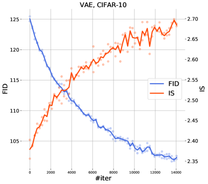
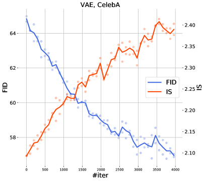
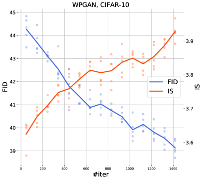
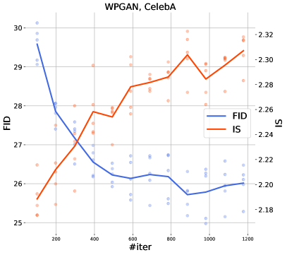
Figure 7: Monotonous improvements in terms of FID and IS for the learning of discriminator by CCE. During iterations, we evaluate metrics $5$ times (scatter) and then average them (solid lines). For a single metric evaluation, we use 10k samples. Higher values of IS and lower values of FID are better. Performance for the original generator corresponds to $0$th iteration of a discriminator.

Appendix I Losses for DRE

Table 2: Different losses for the density-ratio estimation.

PROPOSAL NAME LOSS DRE MARKOV UPPER BOUND (UB) $\displaystyle\int dxdy~{}p(x)q(y\,|\,x)\bigg{[}\log\frac{d(y,x)}{d(x,y)}+\frac{d(y,x)}{d(x,y)}\bigg{]}$ $\displaystyle\frac{p(x)q(y\,|\,x)}{p(y)q(x\,|\,y)}=\frac{d(x,y)}{d(y,x)}$ MARKOV CROSS-ENTROPY (MCE) $\displaystyle\int dxdy~{}p(x)q(y\,|\,x)[-\log d(x,y)-\log(1-d(y,x))]$ $\displaystyle\frac{p(x)q(y\,|\,x)}{p(y)q(x\,|\,y)}=\frac{d(x,y)}{d(y,x)}$ LINEAR TERM (LT) $\displaystyle\int dxdy~{}p(x)q(y\,|\,x)\bigg{[}\frac{d(y,x)}{d(x,y)}\bigg{]}$ $\displaystyle\frac{p(x)q(y\,|\,x)}{p(y)q(x\,|\,y)}=\bigg{(}\frac{d(x,y)}{d(y,x)}\bigg{)}^{2}$ INDEPENDENT UPPER BOUND (UB) $\displaystyle\int dxdy~{}p(x)q(y)\bigg{[}\log\frac{d(y)(1-d(x))}{d(x)(1-d(y))}+\frac{d(y)(1-d(x))}{d(x)(1-d(y))}\bigg{]}$ $\displaystyle\frac{p(x)q(y)}{p(y)q(x)}=\frac{d(x)(1-d(y))}{d(y)(1-d(x))}$ MARKOV CROSS-ENTROPY (MCE) $\displaystyle\int dxdy~{}p(x)q(y)[-\log d(x)(1-d(y))-\log(1-d(y)(1-d(x)))]$ $\displaystyle\frac{p(x)q(y)}{p(y)q(x)}=\frac{d(x)(1-d(y)(1-d(x)))}{(1-d(x))(1-d(x)(1-d(y)))}\cdot$ $\;\;\;\;\;\;\;\;\;\;\;\;\;\;\displaystyle\cdot\frac{(2(1-d(x)(1-d(y)))-d(y))}{((1-d(y)(1-d(x)))+d(y)d(x))}$ LINEAR TERM (LT) $\displaystyle\int dxdy~{}p(x)q(y)\bigg{[}\frac{d(y)(1-d(x))}{d(x)(1-d(y))}\bigg{]}$ $\displaystyle\frac{p(x)q(y)}{p(y)q(x)}=\bigg{(}\frac{d(x)(1-d(y))}{d(y)(1-d(x))}\bigg{)}^{2}$ CONVENTIONAL CROSS-ENTROPY (CCE) $\displaystyle\int dxdy~{}p(x)q(y)[-\log d(x)(1-d(y))]$ $\displaystyle\frac{p(x)q(y)}{p(y)q(x)}=\frac{d(x)(1-d(y))}{d(y)(1-d(x))}$

References

- Arjovsky et al. (2017) Arjovsky, M., Chintala, S., and Bottou, L. Wasserstein gan. arXiv preprint arXiv:1701.07875, 2017.
- Arora & Zhang (2017) Arora, S. and Zhang, Y. Do gans actually learn the distribution? an empirical study. arXiv preprint arXiv:1706.08224, 2017.
- Azadi et al. (2018) Azadi, S., Olsson, C., Darrell, T., Goodfellow, I., and Odena, A. Discriminator rejection sampling. arXiv preprint arXiv:1810.06758, 2018.
- Barratt & Sharma (2018) Barratt, S. and Sharma, R. A note on the inception score. arXiv preprint arXiv:1801.01973, 2018.
- Donahue et al. (2016) Donahue, J., Krähenbühl, P., and Darrell, T. Adversarial feature learning. arXiv preprint arXiv:1605.09782, 2016.
- Goodfellow et al. (2014) Goodfellow, I., Pouget-Abadie, J., Mirza, M., Xu, B., Warde-Farley, D., Ozair, S., Courville, A., and Bengio, Y. Generative adversarial nets. In Advances in neural information processing systems, pp. 2672–2680, 2014.
- Gulrajani et al. (2017) Gulrajani, I., Ahmed, F., Arjovsky, M., Dumoulin, V., and Courville, A. C. Improved training of wasserstein gans. In Advances in Neural Information Processing Systems, pp. 5767–5777, 2017.
- Heusel et al. (2017) Heusel, M., Ramsauer, H., Unterthiner, T., Nessler, B., and Hochreiter, S. Gans trained by a two time-scale update rule converge to a local nash equilibrium. In Advances in Neural Information Processing Systems, pp. 6626–6637, 2017.
- Kingma & Welling (2014) Kingma, D. P. and Welling, M. Auto-encoding variational bayes. ICLR, 2014.
- Ledig et al. (2017) Ledig, C., Theis, L., Huszár, F., Caballero, J., Cunningham, A., Acosta, A., Aitken, A., Tejani, A., Totz, J., Wang, Z., et al. Photo-realistic single image super-resolution using a generative adversarial network. In Proceedings of the IEEE conference on computer vision and pattern recognition, pp. 4681–4690, 2017.
- Neklyudov et al. (2018) Neklyudov, K., Shvechikov, P., and Vetrov, D. Metropolis-hastings view on variational inference and adversarial training. arXiv preprint arXiv:1810.07151, 2018.
- Nowozin et al. (2016) Nowozin, S., Cseke, B., and Tomioka, R. f-gan: Training generative neural samplers using variational divergence minimization. In Advances in Neural Information Processing Systems, pp. 271–279, 2016.
- Paszke et al. (2017) Paszke, A., Gross, S., Chintala, S., Chanan, G., Yang, E., DeVito, Z., Lin, Z., Desmaison, A., Antiga, L., and Lerer, A. Automatic differentiation in pytorch. 2017.
- Pollard (2000) Pollard, D. Asymptopia. Manuscript, Yale University, Dept. of Statist., New Haven, Connecticut, 2000.
- Radford et al. (2015) Radford, A., Metz, L., and Chintala, S. Unsupervised representation learning with deep convolutional generative adversarial networks. arXiv preprint arXiv:1511.06434, 2015.
- Roberts et al. (2004) Roberts, G. O., Rosenthal, J. S., et al. General state space markov chains and mcmc algorithms. Probability surveys, 1:20–71, 2004.
- Salimans et al. (2016) Salimans, T., Goodfellow, I., Zaremba, W., Cheung, V., Radford, A., and Chen, X. Improved techniques for training gans. In Advances in Neural Information Processing Systems, pp. 2234–2242, 2016.
- Turner et al. (2018) Turner, R., Hung, J., Saatci, Y., and Yosinski, J. Metropolis-hastings generative adversarial networks. arXiv preprint arXiv:1811.11357, 2018.
- Yu et al. (2018) Yu, J., Lin, Z., Yang, J., Shen, X., Lu, X., and Huang, T. S. Generative image inpainting with contextual attention. In Proceedings of the IEEE Conference on Computer Vision and Pattern Recognition, pp. 5505–5514, 2018.