Abstract

We now set up Constraint Closure in a manner consistent with Temporal and Configurational Relationalism. This requires modifying the Dirac Algorithm – which addresses the Constraint Closure Problem facet of the Problem of Time piecemeal – to the TRi-Dirac Algorithm. This is a member of the wider class of Dirac-type algorithms that enjoys the property of being Temporal Relationalism implementing (TRi). Constraint algebraic structures ensue. We include examples of types of constraint, outcomes of the Dirac Algorithm and different kinds of Constraint Closure Problems. Enough new Principles of Dynamics is required to support this venture that an Appendix on it is provided: differential Hamiltonians, anti-Routhians, and the brackets, state spaces and morphisms corresponding to these.

¹ dr.e.anderson.maths.physics *at* protonmail.com

1 Introduction

This is our seventh Article [68, 69, 70, 71, 72, 73] on the Problem of Time [13, 12, 10, 24, 27, 30, 31, 37, 50, 51, 53, 56, 57, 62, 61, 67] and its underlying Background Independence. Herein, we extend Articles V and VI’s consistent unified treatment of Article I’s Temporal Relationalism and Article II’s Configurational Relationalism to consistently deal with Constraint Closure as well.

Having introduced Field Theory since Article III’s finite account, the Finite–Field portmanteau notation for constraints is

$$\mbox{\boldmath\scriptsize${\cal C}$}\mbox{ }:=\mbox{ }{\mathscr{F}}\lfloor\mbox{{\bf Q}},\mbox{{\bf P}}\rfloor\mbox{ }:\mbox{ }\mbox{F}(\mbox{\boldmath$Q$},\mbox{\boldmath$P$})\mbox{ }\mbox{ (finite) }\mbox{ }\mbox{ and }\mbox{ }{\cal F}(\underline{x};\mbox{\bf Q},\mbox{\bf P}]\mbox{ }\mbox{ (field) }.$$ (1)

The combination of working in Hamiltonian variables $(\mbox{{\bf Q}},\mbox{{\bf P}})$ and making use of the classical Poisson brackets – extended to portmanteau notation in Sec 2 – turns out to allow for a systematic treatment of constraints: the Dirac Algorithm [10]. We already provided this in Article III; we now generalize this to Dirac-type Algorithms in Sec 3; it is the TRi such that we adopt for Problem of Time facet consistency. We phrase this approach as starting with a trial action ${\cal S}^{\mbox{\scriptsize t}\mbox{\scriptsize r}\mbox{\scriptsize i}\mbox{\scriptsize a}\mbox{\scriptsize l}}$ producing trial constraints. In cases in which Constraint Closure is completed, ‘trial’ names and labels are promoted to ‘CC’ ones, standing for ‘Closure completed’ as well as for the Constraint Closure aspect and facet name. Types of constraint are discussed in Sec 4, and constraint algebraic structures in Sec 5.

Constraint Closure - the third Background Independence aspect - is itself considered in Sec 6. Complications and impasses with this are the corresponding third facet of the Problem of Time: the Constraint Closure Problem.

Functional Evolution Problem was the facet name used by Kuchař and Isham [30, 31] in the quantum-level field-theoretic setting. Some parts of this problem, however, already occur in finite examples, for which partial rather than functional derivatives are involved.

Partional Evolution Problem is thus a more theory-independent portmanteau name for this facet.

Constraint Closure Problem is a more general facet name through its additionally covering the classical version of the problem to some extent.

As useful recollection and for reference, some parts of Problem of Time facet composition between Constraint Closure and Temporal and Configurational Relationalism already given in Article III are as follows.

The split Constraint Provider input has, on the one hand, Temporal Relationalism provides a constraint ${\cal C}$hronos that is quadratic and so is also denoted by ${\cal Q}$uad. On the other hand, Configurational Relationalism provides candidate ${\cal S}$huffle constraints that are linear and so are also denoted by ${\cal L}$in. One is then to use the Dirac Algorithm on this combined incipient set of constraints to see whether Constraint Closure is met or the Constraint Closure Problem arises. This split induces a further split consideration of Constraint Closure: whether each of ${\cal C}$hronos and ${\cal S}$huffle are self first-class, and whether they are mutually first-class. The self and mutual behaviour of ${\cal S}$huffle determines whether Configurational Relationalism has succeeded. Let us also point to the useful ‘end summary road map’ Fig 5 as regards keeping track of how these various facet interferences fit together.

Enough new Principles of Dynamics is required to support this venture to merit an Appendix. This covers differential Hamiltonians, ordial [73] differential almost-Hamiltonians, anti-dRouthians, Peierls brackets [6] and mixed Poisson–Peierls brackets, and the corresponding state spaces and morphisms.

2 Poisson brackets and phase space

Structure 1 As a first instance of Equipping with Brackets, consider the joint space of the Q and P alongside the classical Poisson brackets

$$\mbox{\bf\{}F\mbox{\bf,}\,G\mbox{\bf\}}\mbox{ }:=\mbox{ }\int_{\mbox{\scriptsize N}\mbox{\scriptsize o}\mbox{\scriptsize S}}\textrm{d}\mbox{N}\mbox{o}\mbox{S}\left\{\frac{\mbox{\boldmath$\delta$}\partial F}{\mbox{\boldmath$\delta$}\partial\mbox{{\bf Q}}}\cdot\frac{\mbox{\boldmath$\delta$}\partial G}{\mbox{\boldmath$\delta$}\partial\mbox{{\bf P}}}-\frac{\mbox{\boldmath$\delta$}\partial F}{\mbox{\boldmath$\delta$}\partial\mbox{{\bf P}}}\cdot\frac{\mbox{\boldmath$\delta$}\partial G}{\mbox{\boldmath$\delta$}\partial\mbox{{\bf Q}}}\right\}\mbox{ },$$ (2)

i.e. the portmanteau of (III.1) for finite theories and

$$\mbox{\bf\{}F\mbox{\bf,}\,G\mbox{\bf\}}\mbox{ }:=\mbox{ }\int_{\mbox{\scriptsize\boldmath$\Sigma$}}\textrm{d}\mbox{\boldmath$\Sigma$}\left\{\frac{\updelta F}{\updelta\mbox{\bf Q}}\cdot\frac{\updelta G}{\delta\mbox{\bf P}}-\frac{\updelta F}{\updelta\mbox{\bf P}}\cdot\frac{\updelta G}{\delta\mbox{\bf Q}}\right\}$$ (3)

for Field Theories.

The fundamental Poisson bracket is

$$\mbox{\bf\{}\underline{\mbox{{\bf Q}}}\mbox{\bf,}\,\underline{\mbox{{\bf P}}}\mbox{\bf\}}\mbox{ }=\mbox{ }\underline{\underline{\mbox{\boldmath$\delta$}}}$$ (4)

for $\delta$ the portmanteau of the finite Kronecker $\delta$ and the product of a species-wise such with a field-theoretic Dirac $\updelta^{(d)}(\underline{x}-\underline{x}^{\prime})$. This bracket being established for all the Q and P means that brackets of all once-differentiable quantities ${\mathscr{F}}\lfloor\mbox{{\bf Q}}$, $\mbox{{\bf P}}\rfloor$ are established as well.

Remark 1 The entries into each slot of the Poisson brackets could also be functionals ${\mathscr{F}}$, ${\mathscr{G}}$ rather than just functions $F$, $G$.

Structure 1 In terms of Poisson brackets, the equations of motion are

$$\dot{\mbox{{\bf Q}}}=\mbox{\bf\{}\mbox{{\bf Q}}\mbox{\bf,}\,{\mathscr{H}}\mbox{\bf\}}\mbox{ },\mbox{ }\mbox{ }\dot{\mbox{{\bf P}}}=\mbox{\bf\{}\mbox{{\bf P}}\mbox{\bf,}\,{\mathscr{H}}\mbox{\bf\}}\mbox{ }.$$ (5)

Structure 2 Thus equipped, this joint space is known as phase space, $\mathfrak{P}$hase.

Remark 2 Our first preoccupation is establishing which structures are already TRi, and which need to be supplanted by TRi counterparts. The Poisson bracket is already-TRi. (5) becomes

$$\mbox{\bf d}\partial{\mbox{{\bf Q}}}=\mbox{\bf\{}\mbox{{\bf Q}}\mbox{\bf,}\,{\mathscr{H}}\mbox{\bf\}}\mbox{ },\mbox{ }\mbox{ }\mbox{\bf d}\partial{\mbox{{\bf P}}}=\mbox{\bf\{}\mbox{{\bf P}}\mbox{\bf,}\,{\mathscr{H}}\mbox{\bf\}}\mbox{ }.$$ (6)

$\mathfrak{P}$hase is already-TRi, since all of $Q$, $P$ and the Poisson bracket are.

Structure 3 The Liouville 1-form

$$\mbox{\boldmath$P$}\cdot\mbox{\bf d}\partial\mbox{\boldmath$Q$}$$ (7)

and the symplectic 2-form

$$\mbox{\bf d}\partial\mbox{\boldmath$P$}\wedge\mbox{\bf d}\partial\mbox{\boldmath$Q$}$$ (8)

– each further motivated in Appendix A.4 – are relatively rare examples of already-TRi objects of nonzero weight: change 1- and 2-forms respectively. See the Appendix for some of their further significance.

As the inverse of the previous, the Poisson tensor $C$ is recast as a change 2-tensor $d^{-2}\mbox{\boldmath$D$}$.

Structure 4 Temporal Relationalism also requires use of specifically time-independent canonical transformations $Can$ rather than the more general $Can_{t}$ (see Appendix A.4) in the $d$-Hamiltonian formulation.

3 Dirac-type Algorithm

3.1 TRi appending via cyclic differentials

Remark 1 One part of handling constraints is to additively append them to a bare Hamiltonian-type object. For this to attain TRi, the bare object is to be a differential Hamiltonian

$$\mbox{\bf d}\partial{\mathscr{H}}\mbox{ }.$$ (9)

and the appending is to be done not with cyclic differentials in place of Dirac’s Lagrange multipliers.

Structure 1 The TRi Dirac-type Algorithm requires declaring differential-almost-Hamiltonian variables: $(\mbox{{\bf Q}},\mbox{{\bf P}})$ in the part-physical sector and $\mbox{\bf d}\partial\mbox{\bf A}$ in the purely auxiliary sector.

Definition 1 The arbitrary-primary differential-almost-Hamiltonian (alias Dirac-type ‘starred’ differential-almost-Hamiltonian) is

$$\mbox{\bf d}\partial{\mathscr{A}}_{\mbox{\scriptsize\boldmath$A$}\mbox{\boldmath\tiny${\cal P}$}}:=\mbox{\bf d}\partial{\mathscr{A}}^{*}:=\mbox{\bf d}\partial{\mathscr{H}}+\mbox{\bf d}\partial\underbracket{\mbox{\bf A}}\cdot\underbracket{\mbox{\boldmath\scriptsize${\cal P}$}}\mbox{ }.$$ (10)

I.e.  the result of taking a bare differential Hamiltonian $\mbox{\bf d}\partial\mbox{H}$ and additively appending to it a theory’s formalism’s primary constraints ${\cal P}$ using arbitrary functions of $(\mbox{{\bf Q}},\mbox{{\bf P}})$ now represented as cyclic differentials $\textrm{d}\mbox{\bf A}(\mbox{{\bf Q}},\mbox{{\bf P}})$.

Definition 2 The unknown-primary differential-almost-Hamiltonian (alias Dirac-type total differential-almost-

Hamiltonian) is

$$\mbox{\bf d}\partial{\mathscr{A}}_{\mbox{\scriptsize\boldmath$u$}\mbox{\boldmath\tiny${\cal P}$}}:=\mbox{\bf d}\partial{\mathscr{A}}_{\mbox{\scriptsize T}}:=\mbox{\bf d}\partial{\mathscr{H}}+\mbox{\bf d}\partial\underbracket{\mbox{{\bf u}}}\cdot\underbracket{\mbox{\boldmath\scriptsize${\cal P}$}}\mbox{ }.$$ (11)

I.e. the result of additively appending the same but now using unknown cyclic differentials $\mbox{\bf d}\partial\mbox{{\bf u}}(\mbox{{\bf P}},\mbox{{\bf Q}})$.

Remark 3 As an indication of how the preceding definition is used,

$$0\mbox{ }\approx\mbox{ }\mbox{\bf d}\partial\mbox{\boldmath\scriptsize${\cal P}$}\mbox{ }=\mbox{ }\mbox{\bf\{}\mbox{\boldmath\scriptsize${\cal P}$}\mbox{\bf,}\,\mbox{\bf d}\partial{\mathscr{A}}_{\mbox{\scriptsize\boldmath$u$}\mbox{\boldmath\tiny${\cal P}$}}\mbox{\bf\}}\mbox{ }=\mbox{ }\mbox{\bf\{}\mbox{\boldmath\scriptsize${\cal P}$}\mbox{\bf,}\,\mbox{\bf d}\partial{\mathscr{H}}\mbox{\bf\}}+\mbox{\bf\{}\mbox{\boldmath\scriptsize${\cal P}$}\mbox{\bf,}\,\underbracket{\mbox{\boldmath\scriptsize${\cal P}$}}\mbox{\bf\}}\cdot\mbox{\bf d}\partial\underbracket{\mbox{{\bf u}}}\mbox{ }.$$ (12)

The first step is dictated by consistency, the second by the differential-almost-Hamilton’s equations (Appendix A.1), and the third by definition and linearity.

Remark 4 For Field Theories with fields $\uppsi$ and allowing for the spatial metric h to be among these, we also now require TRi-smearing for our constraints:

$$(\underline{\mbox{{\boldmath\scriptsize${\cal C}$}}}\,|\,\partial\underline{\mbox{\bf W}})\mbox{ }:=\mbox{ }\int d^{3}x\,\underline{\mbox{{\boldmath\scriptsize${\cal C}$}}}(\underline{x};\mbox{\bf h},\mbox{\boldmath$\uppsi$},\mbox{\bf p},\mbox{\boldmath$\uppi$}^{\uppsi}]\,\partial\mbox{\bf W}(\underline{x})\mbox{ }.$$ (13)

Such expressions are then inserted inside the classical brackets.

Remark 5 The brackets in use are now the physical Poisson brackets sector of a mixed Poisson–Peierls bracket (Appendix A.7) as is appropriate to the corresponding unreduced ordial-almost-phase space $\mbox{\bf d}\partial\mbox{A}$-$\mathfrak{P}$hase rather than phase space $\mathfrak{P}$hase.

The complementary Peierls sector (Appendix [6]) is purely-auxiliary, and so is just ‘unphysical fluff’.

This split is guaranteed by constraints being of the form $\mbox{\scriptsize${\cal C}$}(\mbox{{\bf Q}},\mbox{{\bf P}}\mbox{ alone})$, because

$$\mbox{passage from $\mbox{\bf d}\partial\mbox{{\bf Q}}$ to $\mbox{{\bf P}}$ absorbs all the $\mbox{\bf d}\partial\mbox{\tt g}$}\mbox{ }.$$ (14)

This is the major trick which can be performed with Appendix A.2’s ($\mbox{\bf d}\partial$-)anti-Routhian.

Remark 6 The resultant equation (12) is an explicit equation, with the cyclic differential auxiliaries $\mbox{\bf d}\partial\mbox{\boldmath$u$}$ playing the role of unknowns.

Remark 7 Since only the Poisson bracket part acting on the constraints, the definitions of first- and second-class remain unaffected, as are the Dirac bracket and the extension procedure.

Remark 8 See Fig 6 for some context. Phase space $\mathfrak{P}$hase is now replaced by A-$\mathfrak{P}$hase and $\mbox{\bf d}\partial$A-$\mathfrak{P}$hase; these are all types of bundle twice over: cotangent bundles and $\mathfrak{g}$-bundles. Locally (in configuration space) product spaces will do.

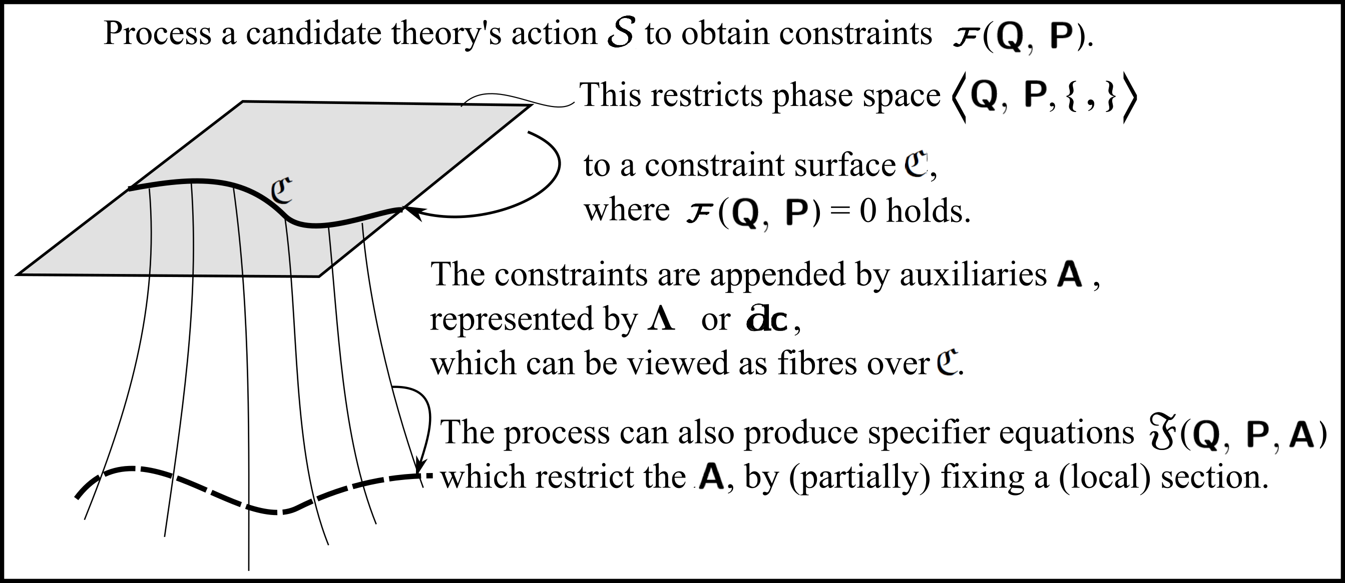
Figure 1: Geometrical sketch of the outcome of Dirac-type procedures for classical Constraint Closure. We omit a loop back to readjusting some of the phase space structures – Q, P and classical bracket – in the event of second-class constraints arising. While the Dirac Algorithm’s Lagrange multipliers $\Lambda$ can be incorporated by extending the Q, the TRi-Dirac-type Algorithm’s cyclic differentials d$\partial$C are more heterogeneous. In any case, envisaging the auxiliary variables used in Constraint Appending as fibres keeps them separated out from the phase space which contains actual physical information. [See Part III of [61] for comparison with the simpler assessment of Constraint Closure at the quantum level.]

3.2 TRi Dirac Little Algorithm

Dirac’s Algorithm is moreover not TRi because the appending Lagrange multipliers break this. It is, instead, supplanted by the TRi-Dirac Algorithm in which appending is performed by cyclic differentials.

As regards the six cases this is capable of producing at each step (c.f. Article III), in any combination, equation types 0), 1) and 3) are as before. On the other hand, equation types 2) and 3) are now phrased in terms of cyclic differentials.

Definition 1 The TRi-Dirac Little Algorithm [10] consists of evaluating classical brackets between a given set of constraints so as to determine whether these are consistent and complete.

At this level, four types of equation can emerge.

Type 0) Inconsistencies.

Type 1) Mere identities.

Type 2) Further secondary constraints, i.e. equations independent of the cyclic differential unknowns.

Type 3) Specifier equations, i.e. relations amongst some of the appending cyclic differential functions themselves.

Remark 1 The possibility of specifier equations stems from the TRi Dirac Algorithm involving an appending procedure involving such auxiliaries. As already mentioned in Article III, the Dirac Algorithm itself involves restrictions on Lagrange multiplier auxiliaries.

Remark 2 Dirac-type algorithms moreover generalize the type of appending auxiliaries; The TRi-Dirac Algorithm subcase involves, concretely, cyclic differential auxiliaries. So we now extend the single-facet notion of ‘specifier equation’ from Lagrange multiplier auxiliaries to this more general context.

3.3 Discussion

Remark 1 Article III’s uses of ((nontrivial) ab initio) consistent carry over.

Remark 2 First- and second-classness carry over within the physical Poisson sector, as does closure under Poisson brackets as a completeness criterion. We again postpone the possibility of second-classness to Sec 3.6, the TRi-Dirac Little Algorithm itself operating under the aegis that all constrains involved are first-class.

Remark 3 If type 2) occurs, these first-class constraints are fed into the subsequent iteration of the algorithm.

This is by, firstly, defining ${\cal Q}$ as one’s initial ${\cal P}$ alongside the ${\cal R}$ subset of the candidate theory’s formulation’s ${\cal S}$ that have been discovered so far, indexed by $\mbox{Q}=\mbox{P}\coprod\mbox{R}$.

Secondly, by restarting from a more general form for our problem (12)

$$0\approx\mbox{\bf d}\partial{\mbox{\scriptsize${\cal Q}$}}\mbox{ }=\mbox{ }\mbox{\bf\{}\mbox{{\boldmath\scriptsize${\cal Q}$}}\mbox{\bf,}\,\mbox{\bf d}\partial{\mathscr{A}}_{\mbox{\scriptsize\boldmath$u$}\mbox{{\boldmath\scriptsize${\cal Q}$}}}\mbox{\bf\}}\mbox{ }=\mbox{ }\mbox{\bf\{}\mbox{{\boldmath\scriptsize${\cal Q}$}}\mbox{\bf,}\,\mbox{\bf d}\partial{\mathscr{H}}\mbox{\bf\}}+\mbox{\bf\{}\mbox{{\boldmath\scriptsize${\cal Q}$}}\mbox{\bf,}\,\underbracket{\mbox{{\boldmath\scriptsize${\cal Q}$}}}\mbox{\bf\}}\cdot\mbox{\bf d}\partial\underbracket{\mbox{\boldmath$u$}}\mbox{ }.$$ (15)

Proceed recursively until one of the following termination conditions is attained.

Termination Condition 0) Immediate inconsistency due to at least one inconsistent equation arising.

Termination Condition 1) Combinatorially critical cascade. This is due to the iterations of the TRi-Dirac Algorithm producing a cascade of new objects down to the ‘point on the surface of the bottom pool’ that leaves the candidate with no degrees of freedom. This has the status of a combinatorial triviality condition.

Termination Condition 2) Sufficient cascade. This runs ‘past the surface of the bottom pool’ of no degrees of freedom into the ‘depths of inconsistency underneath’.

Termination Condition 3) Completion is that the latest iteration of the TRi-Dirac Algorithm has produced no new nontrivial consistent equations, indicating that all of these have been found.

Remark 4 Our input candidate set of generators is either itself complete or incomplete – ‘nontrivially TRi-Dirac’ – depending on whether it does not or does imply any further nontrivial objects. If it is incomplete, it may happen that the TRi-Dirac Algorithm provides a completion, by only an combinatorially insufficient cascade arising, from the point of view of killing off the candidate theory.

Remark 5 So, on the left point of the trident, Termination Condition 3) gives a Closure acceptance condition for an initial candidate set of constraints alongside the cascade of further objects emanating from it by the TRi-Dirac Algorithm. I.e. one demonstrates a ‘TRi-Dirac completion’ of the incipient candidate set of constraints.

Remark 6 On the right point of the trident, Termination Conditions 0) and 2) are rejections thereof.

Remark 7 On the final middle point of the trident, Termination Condition 1) remains the critical edge case.

Remark 8 In detailed considerations, clarity is often improved by labelling each iteration’s ${\cal R}$ and ${\cal Q}$ by the number of that iteration. In the case of completion being attained, (the final ${\cal R}$) = ${\cal S}$ itself – all the first-class secondary constraints – whereas $\mbox{{\boldmath\scriptsize${\cal Q}$}}=\mbox{{\boldmath\scriptsize${\cal F}$}}$: all the first-class constraints.

Remark 7 We now have enough space to comment that, firstly, Dirac’s own description of specifier equation was [10] ‘imposes a condition’.

Secondly, that the term ‘fixing equations’, as in e.g. ‘lapse fixing equation’, is often used for in Numerical Relativity. C.f. maximal and constant mean curvature lapse fixing equations in this context. This useage is however a subcase of gauge-fixing, nor does all gauge-fixing involves specification of Lagrange multipliers. E.g. Lorenz gauge need not be interpreted in this way. On these grounds, the distinct name ‘specifier equations’ is used in this Series.

3.4 Each iteration’s problem is a linear system

Remark 1 (12) or its subsequent-iteration generalization (15) is, once again, a linear problem.

Its general solution – now a cyclic differential – thus splits according to

$$\mbox{\bf d}\partial\mbox{\boldmath$u$}=\mbox{\bf d}\partial\mbox{\boldmath$p$}+\mbox{\bf d}\partial\mbox{\boldmath$C$}\mbox{ },$$ (16)

for particular solution $\mbox{\bf d}\partial\mbox{\boldmath$p$}$ and complementary function $\mbox{\bf d}\partial\mbox{\boldmath$C$}$.

By definition, $\mbox{\bf d}\partial\mbox{\boldmath$C$}$ solves the corresponding homogeneous equation

$$\mbox{\bf d}\partial\underbracket{\mbox{\boldmath$C$}}\cdot\mbox{\bf\{}\underbracket{\mbox{{\boldmath\scriptsize${\cal C}$}}}\mbox{\bf,}\,\mbox{\boldmath\scriptsize${\cal P}$}\mbox{\bf\}}\approx 0\mbox{ }.$$ (17)

$C$ furthermore has the structure

$$\mbox{\bf d}\partial\underbracket{\mbox{\boldmath$C$}}=\mbox{\bf d}\partial\underbracket{\mbox{\boldmath$c$}}\,\underbracket{\underbracket{\mbox{\boldmath$R$}}}\mbox{ }.$$ (18)

The $\mbox{\bf d}\partial\mbox{\boldmath$c$}$ here are the totally arbitrary coefficients of the independent solutions, whereas $R$ is again a mixed-index and thus in general rectangular matrix, just as it was in Article III. Our general solution’s destintion is to be substituted into the total differential almost-Hamiltonian, updating it.

3.5 TRi-Dirac appending of cyclic differentials. ii)

Definition 1 particular-primary differential-almost-Hamiltonian (alias Dirac-type primed differential-almost)

-Hamiltonian is

$$\mbox{\bf d}\partial{\mathscr{A}}_{\mbox{\scriptsize\boldmath$p$}\mbox{\boldmath\tiny${\cal P}$}}:=\mbox{\bf d}\partial{\mathscr{A}}^{\prime}:=\mbox{\bf d}\partial{\mathscr{H}}+\mbox{\bf d}\partial\underbracket{\mbox{\boldmath$p$}}\cdot\underbracket{\mbox{\boldmath\scriptsize${\cal P}$}}\mbox{ }.$$ (19)

Definition 2 The differential-almost-Hamiltonian with first-class constraints appended (alias Dirac-type extended differential-almost-Hamiltonian) is

$$\mbox{\bf d}\partial{\mathscr{A}}_{\mbox{\bf\tiny${\cal F}$}}:=\mbox{\bf d}\partial{\mathscr{A}}_{\mbox{\scriptsize E}}:=\mbox{\bf d}\partial{\mathscr{H}}+\mbox{\bf d}\partial\underbracket{\mbox{\boldmath$u$}}\cdot\underbracket{\mbox{\boldmath\scriptsize${\cal P}$}}+\mbox{\bf d}\partial\underbracket{\mbox{\boldmath$a$}}\cdot\underbracket{\mbox{\boldmath\scriptsize${\cal S}$}}\mbox{ }.$$ (20)

These d$a$ are arbitrary functions, and these ${\cal S}$ are specifically first-class secondary constraints. The description leaves it implicit that those auxiliaries which can be solved for, are solved for.

Remark 1 Such a notion could clearly be declared for each iteration of the TRi-Dirac Algorithm, with the above one coinciding with the TRi-Dirac Little Algorithm attaining completeness. In this sense, $\mbox{\bf d}\partial{\mathscr{A}}_{\mbox{\bf\tiny${\cal F}$}}$ is itself a candidate theory’s maximally extended differential-almost-Hamiltonian. This places order-theoretic content in the TRi-Dirac multiplicity of differential almost-Hamiltonians. It is $\mbox{\bf d}\partial{\mathscr{A}}_{\mbox{\bf\tiny${\cal F}$}}$ that supplants the GR extended Hamiltonian, itself a truer name for the notion that most of the literature calls ‘GR total Hamiltonian’.

3.6 Removing second-class constraints

Suppose second-class constraints arising at some iteration in the TRi-Dirac Algorithm. Three different approaches to this are as follows.

Procedure A) Remove these by replacing the incipient Poisson brackets with Dirac brackets ([10] and already covered in Article III).

Procedure B) Extend $\mathfrak{P}$hase with further auxiliary variables so as to ‘gauge-unfix’ second-class constraints into first-class ones [28, 29].

Procedure C) Remove the objects in question by Lagrangian-level reduction.

Universality criterion 1 Whereas procedures A) and B) are both in principle systematically available, C) is not, though it is solvable for this Series of Articles’s RPM and SIC examples. Second-class constraints can moreover always in principle be handled locally by thinking about them instead as ‘already-applied’ gauge fixing conditions that can be recast as first-class constraints by adding suitable auxiliary variables. By this procedure, a system with first- and second-class constraints extends to a more redundant description of a system with just first-class constraints.

Remark 1 As regards A), suppose second-class constraints are present at some iteration in the TRi-Dirac Algorithm.

Structure 2 The preceding can moreover happen on subsequent iterations of the TRi-Dirac Algorithm, were these to reveal more second-class constraints. I.e. while still in the process of investigating a physical theory’s constraints, one does not yet know which are first-class. This is because a given constraint may close with all the constraints found so far but not close with some constraint still awaiting discovery. Thus one’s characterization of constraints needs to be updated step by step until either of the following apply.

The notion of final classical bracket alias maximal Dirac bracket thus also carries over as already-TRi.

3.7 Various notions of gauge

Remark 1 Some constraints are regarded as gauge constraints. In general, however, exactly which kinds of constraints these comprise remains disputed in the literature.

Remark 2 One point agreed upon is that a Gauge Theory has an associated group $\mathfrak{g}$ of transformations that are held to be unphysical. The above-mentioned disjoint auxiliary variables often constitute the generators of such a group.

Remark 3 Another point that is agreed upon is that second-class constraints are not gauge constraints; all gauge constraints use up two degrees of freedom.

Dirac’s Conjecture [10] is that, a fortiori, all first-class constraints are gauge constraints.

By this, using up two degrees of freedom would conversely imply being a gauge constraint.

Sec 4 however details that Dirac’s conjecture has long been known to be false [29].

Remark 4 What the gauge group acts upon is another source of diversity.

Definition 1 ‘Gauge Theory’ in Dirac’s sense [4, 10] applies to data at a given time. A true-name for gauge in this case is thus data-gauge.

Definition 2 ‘Gauge Theory’ in Bergmann’s sense [8] applies to data along whole paths, i.e. trajectories in spacetime. A true-name for gauge in this case is thus path-gauge.

Remark 5 One may extend the first of these to a fork between timeless configurations, configuration–velocity, configuration-change, and phase space versions of data.

Remark 6 One may extend the second to make further distinction between paths and histories; see Part II of [61] for details on all of these distinctions.

Remark 7 Make careful distinction between different notions of Gauge Theory as here, and the more familiar issue of making particular choices of gauge within the one notion of gauge, such as working in Lorenz gauge for Electromagnetism.

Remark 8 In the current Article, ‘gauge’ is meant in Dirac’s ‘data-gauge’ sense, as is appropriate to canonical approaches see Article X for its use in Bergmann’s ‘path gauge’ sense in spacetime approaches.

Remark 9 Sec 4 and Article X moreover contain further GR or gravitational theory specific issues with the extent to which Gauge Theory ideas permeate into, or suffice for, Gravitation.

3.8 Discussion

Remark 1 Each of procedures A) to C) render it clear that whether a theory exhibits second-class constraints is in fact a formulation-dependent statement. As such, the current Series’ previous mentions of ‘formulations of theories’ in connection to sets of constraints are indeed not superfluous.

Remark 2 Gauge-fixing conditions

$$\mbox{\boldmath${\cal X}$}\mbox{ }\mbox{ with components }\mbox{ }{\cal X}_{\mbox{{\scriptsize X}}}$$ (21)

may be applied to whatever Gauge Theory (for all that final answers to physical questions are required to be gauge-invariant).

Remark 3 Of relevance to footnote 3, the square in Fig 2 does not in general commute (see e.g. [43]).

Figure 2: The in general noncommuting square of Legendre transformations (horizontal) and reductions (vertical) in a) plain and b) TRi settings.

Remark 4 Also as regards footnote 3, at least in the more standard theories of Physics, first-class secondary constraints can be taken to arise from variation with respect to mathematically disjoint auxiliary variables. The effect of this variation is to additionally use up part of an accompanying mathematically-coherent block of variables that otherwise contains partially physical information.

3.9 TRi Dirac Full Algorithm

Proceed as in Sec 3.2, except that whenever second-class constraints appear, one switches to (new) Dirac brackets that factor these in. This amounts to the possibility of a fifth type of equation, in parallel with Sec III.2.11.

Type 4) Further second-classness may arise.

Aside 1 Let us distinguish between auxiliaries used for appending and smearing variables. The latter are more widely applicable since their job – ‘multiplication by a test function’ – is to render rigorous a wider range of ‘distributional’ manipulations provided that these occur within an integral. In particular, this applies to classical Field Theories’ Assignment of Observables (for which there is no appending procedure).

Aside 2 For later convenience, we express the ${\cal F}$lin in manifestly homogeneous linear form:

$$\mbox{\scriptsize${\cal F}$}\mbox{lin}_{\mbox{{\scriptsize N}}}={\cal F}[\mbox{{\bf Q}}]^{\mbox{{\scriptsize A}}}\mbox{}_{\mbox{{\scriptsize N}}}\mbox{P}_{\mbox{{\scriptsize A}}}\mbox{ }.$$ (22)

This includes the possibility of ${\cal F}$ being differential operator-valued so as to accommodate Electromagnetism, Yang–Mills Theory and GR.

Remark 1 At each iteration, then, one ends up with a bare differential Hamiltonian with first-class constraints appended using cyclic differentials. The final such is once again denoted by $\textrm{d}{\mathscr{A}}_{\mbox{\bf\tiny${\cal F}$}}$, corresponding to having factored in all second-class constraints and appended all first-class constraints. Each other notion of differential almost Hamiltonian above can also be redefined for Dirac brackets, whether maximal or at any intermediary stage.

Remark 2 As the endpoint of our elaboration of ‘extended Hamiltonians’ along Dirac’s lines, on the one hand, and TRi on the other, we accord this object it a more compact final name for future reference, namely ‘Rid-amiltonian’. On the one hand, this builds in that this is not just TRi but Ri: Relationalism implementing. On the other hand, ‘amiltonian’ is short for an almost-Hamiltonian (c.f. transforming between Hamiltonians sometimes being phrased as from a Hamiltonian to a transformed Kamiltonian). ‘d-amiltonian’ is, similarly, short for a differential-almost-Hamiltonian. We preserve our notation ‘d A’ notation for this final concept, by using

$$\mbox{\bf d}\partial{\mathscr{A}}_{\mbox{\scriptsize R}\mbox{\scriptsize i}}\mbox{ }$$ (23)

and that e.g. ${\cal S}_{\mbox{\scriptsize J}}$: is Jacobi action, so the subscript comes first in the corresponding naming. This is technically a three-aspect object: a Ri-object that additionally belongs to the machinery of testing for Closure. It is not however yet a three-aspect-incorporating object; if it were, its subscript would be ‘CC-Ri’; it is only promoted to this stage when the TRi-Dirac Algorithm has confirmed its pertinence to a consistent theory.

Type 5 Discovery of topological obstructions also carries over mathematically unaltered to the TRi setting. We present a more extensive discussion of such matters in Article XIV.

4 Examples of distinctions between types of constraint

Let us next justify the finer distinctions between types of constraint made in Article III.

Example 1) The constraints considered so far in this Series of Articles – in particular RPM’s $\underline{\mbox{\boldmath\scriptsize${\cal P}$}}$, $\underline{\mbox{\boldmath\scriptsize${\cal L}$}}$, ${\cal D}$, ${\cal E}$, Electromagnetism’s ${\cal G}$, Yang–Mills Theory’s $\mbox{\scriptsize${\cal G}$}_{I}$, and GR-as-Geometrodynamics’ $\underline{\mbox{{\boldmath\scriptsize${\cal M}$}}}$, ${\cal H}$ – are all first-class. It is thus useful to now provide examples of second-class constraints, so that readers see that these do in fact reside in some familiar theories which are either standard observationally substantiated theories, or just one step therefrom.

i) In the $\mbox{\boldmath$Q$}=(\mbox{A}_{i},\Phi)$ formulation of the ‘massive analogue of Electromagnetism’ (alias Proca Theory),

$$\mbox{\scriptsize${\cal C}$}:=\mbox{\boldmath$\partial$}\cdot\mbox{\bf E}+m^{2}\Phi=0\mbox{ }.$$ (24)

This indeed uses up only one degree of freedom, so this theory has one more physical mode than Electromagnetism itself (from two transverse-traceless modes to having a longitudinal mode as well).

ii) Specifically Gravitational Theories with second-class constraints include Einstein–Dirac Theory (i.e. GR with spin-1/2 fermion matter) [35] and Supergravity [21].

For the first four theories above, the absence of second-class constraints means that the Dirac chain consists of just the incipent Poisson bracket itself. I.e. the single-element chain, for which the bottom and top elements coincide, so the maximal Dirac bracket is just this case’s incipient Poisson bracket.

For Proca Theory, however, precisely 1 step in the Dirac(-type) Algorithm produces a second-class constraint, so the Dirac chain consists of the incipient Poisson bracket followed by the final maximal Dirac bracket.

We finally leave finding the simplest and most mundane examples of Dirac chains with nontrivial middle as an exercise for the readers.

Example 2) Relational recovery of Gauge Theory (in Dirac’s data sense). With Configurational Relationalism’s $\mathfrak{g}$ being a candidate group of physically irrelevant motions, in general it remains to be ascertained whether the ${\cal S}$huffle provided by Best Matching is a gauge constraint ${\cal G}$auge which corresponds to $\mathfrak{g}$.

Remark 1 Whether there is $\mathfrak{g}$ compatibility can at least in part be investigated prior to consideration of constraints.

This is since, on the one hand,

$$\mbox{\bf\{}V\mbox{\bf,}\,P_{\mbox{\normalsize$\mathfrak{g}$}}\mbox{\bf\}}$$ (25)

in

$$\mbox{\bf\{}\mbox{\scriptsize${\cal C}$}\mbox{hronos}\mbox{\bf,}\,P_{\mbox{\normalsize$\mathfrak{g}$}}\mbox{\bf\}}$$ (26)

can already be examined prior to constraints: adopting a $\mathfrak{g}$ comes with Equipping with Brackets.

On the other hand, one does not assess $\mathfrak{T}(\mbox{\Large$\mathfrak{q}$},\dot{\mbox{\Large$\mathfrak{q}$}})$ itself, which is tied to constraints being more simply and systematically handled in Hamiltonian-type formulations.

Remark 2 The ensuing action can be viewed as a map from a structure that is a fibre bundles twice over: both a tangent bundles and $\mathfrak{g}$-fibre bundles. Specifically, it is

$$\mbox{\Large$\mathfrak{p}$}\big{(}\mathfrak{T}(\mbox{\Large$\mathfrak{q}$}),\mbox{\Large$\mathfrak{g}$}\big{)}\mbox{ },$$ (27)

rather than

$$\mathfrak{T}\big{(}(\mbox{\Large$\mathfrak{p}$}(\mbox{\Large$\mathfrak{q}$},\mbox{\Large$\mathfrak{g}$})\big{)}$$ (28)

due to the nontrivial part of the $\mathfrak{g}$ action being on the tangent bundles’ fibres. This being a $\mathfrak{g}$-fibre bundle mathematically can moreover require excision of certain degenerate configurations [65, 66], which in turn is not a relationally bona fide procedure.

Counter-example 3) Despite Dirac’s Conjecture,

$$\mbox{\boldmath\scriptsize${\cal F}$}\mbox{\bf lin}\centernot{\Rightarrow}\mbox{\boldmath\scriptsize${\cal G}$}\mbox{\bf auge}$$ (29)

by e.g. the following technically constructed but not physically motivated counter-example given by Henneaux and Teitelboim [29]. The Lagrangian

$$L=\mbox{$\frac{1}{2}$}\,\mbox{exp}(y)\dot{x}^{2}$$ (30)

gives a constraint

$$p_{x}=0$$ (31)

which is first-class but not associated with any gauge symmetry.

Example 4) Whereas $\underline{\mbox{\boldmath\scriptsize${\cal L}$}}$, ${\cal G}$, $\underline{\mbox{{\boldmath\scriptsize${\cal M}$}}}$ are uncontroversially gauge constraints, the gauge status of ${\cal H}$ and even ${\cal E}$ remain disputed. I.e. ${\cal C}$hronos constraints entail ‘gauge subtleties’. Some arguments of note in this regard have been given by Kuchař , Barbour and Foster [32, 37, 46].

This point is, moreover, directly at odds with [29], which transform to and from constraints of the form ${\cal Q}$uad. The Author pointed out [56] that this discrepancy is due to the following.

On the one hand, [29] allowing for $t$-dependent canonical transformations, $Can_{t}$ (see Appendix A.4).

On the other hand, the relational whole-universe context has no primary-level $t$, by which it is not licit to adopt $Can_{t}$ in this worldview. ${\cal C}$hronos and ${\cal G}$auge are consequently qualitatively distinct in the relational context. The relational context furthermore makes distinction between Constraint Providers for, firstly, ${\cal S}$huffle candidates for ${\cal G}$auge, and, secondly, ${\cal C}$hronos.

Remark 3 It is fitting for Configurational Relationalism to be associated with a data-gauge notion.

Remark 4 GR’s ${\cal H}$ is moreover a case study into the extent to which Gauge Theory ideas permeate into, or suffice for, Gravitation.

i) To what extent is one still dealing with Gauge Theory when groupoid rather than group structure is present? For inclusion of ${\cal H}$ means that one’s first-class constraints locally form not an algebra but an algebroid: the Dirac Algebroid.

ii) To what extent can ‘hidden symmetries’ can be treated as gauge symmetries? This is relevant to ${\cal H}$ since this encodes Refoliation Invariance as a hidden symmetry.

iii) Pons, Salisbury and Sundermeyer [48, 49] argue for GR’s evolution generator mimicking, rather than being, a gauge generator; see Article XII for more about this.

Constraint algebroids and hidden symmetries moreover enter Gravitational Theory beyond GR; see e.g. Sec 6.2.

Counter-example 6) Article XI moreover presents a SIC example of

$$\mbox{\boldmath\scriptsize${\cal G}$}\mbox{\bf auge}\centernot{\Rightarrow}\mbox{\boldmath\scriptsize${\cal F}$}\mbox{\bf lin}\mbox{ },$$ (32)

i.e. failure of a partial converse to Dirac’s Conjecture.

This discussion, by delving into one or both of Gravitational and Background Independent ventures, takes us in a direction considerably outside of the scope of Henneaux and Teitelboim’s excellent book [29].

5 Constraint algebraic structures

5.1 Overview

Structure 1 The end product of a successful candidate theory’s passage through the Dirac Algorithm is a constraint algebraic structure consisting solely of first-class constraints closing under Poisson (or more generally Dirac) brackets.

Remark 1 Article III already covered the general form of this.

Structure 2 We now furthermore identify individual constraint algebraic structures to each be a Poisson algebraic structure in the obvious sense; see e.g. [54] for an introduction to Poisson algebras.

Structure 3 The end product of a successful candidate theory’s passage through the Dirac Algorithm is a constraint algebraic structure consisting solely of first-class constraints closing under Poisson (or more generally Dirac) brackets. This is already-TRi and so carries over.

Structure 4 Sec III.2.17’s lattice of subalgebraic structures is an already-TRi structure as well, and so also carries over.

5.2 Examples of constraint algebraic structures

Cases with reduction at any classical level explicitly attained are aided in the matter of closure by one or both of the following means.

Means a) Having fewer constraints to form brackets out of.

Means b) Making use of single finite-theory classical constraints always Abelianly closing with themselves by symmetric entries into an antisymmetric bracket.

Example 0) Minisuperspace has just one constraint, $\mbox{\scriptsize${\cal C}$}\mbox{hronos}=\mbox{\scriptsize${\cal H}$}_{\mbox{\scriptsize m}\mbox{\scriptsize i}\mbox{\scriptsize n}\mbox{\scriptsize i}}$, so we have

$$\mbox{\bf\{}\mbox{\scriptsize${\cal H}$}_{\mbox{\scriptsize m}\mbox{\scriptsize i}\mbox{\scriptsize n}\mbox{\scriptsize i}}\mbox{\bf,}\,\mbox{\scriptsize${\cal H}$}_{\mbox{\scriptsize m}\mbox{\scriptsize i}\mbox{\scriptsize n}\mbox{\scriptsize i}}\mbox{\bf\}}=0\mbox{ }:$$ (33)

closure as a single-generator Abelian Lie algebra. It thereby passes all kinds of Constraint Closure.

Example 1.R) Reduced Euclidean RPM also has just one constraint, $\mbox{\scriptsize${\cal C}$}\mbox{hronos}=\widetilde{\mbox{\scriptsize${\cal E}$}}$, so we once again attain Constraint Closure in the algebraic form

$$\mbox{\bf\{}\widetilde{\mbox{\scriptsize${\cal E}$}}\mbox{\bf,}\,\widetilde{\mbox{\scriptsize${\cal E}$}}\mbox{\bf\}}=0\mbox{ }.$$ (34)

This has the added merit that Configurational Relationalism has been incorporated (minisuperspace did not have any of this to begin with).

Example 1.U) Unreduced Euclidean RPM has the constraint algebra described in Sec III.2.18.

Reduced similarity RPM obeys (34) for redefined $\widetilde{\mbox{\scriptsize${\cal E}$}}$ as well. Note that explicit reduction is easy in 1-$d$, solved with a bit of geometry in 2-$d$, and yet manifests much harder topology and geometry for $\geq 3$-$d$, with solutions at best local in $\widetilde{\mbox{\Large$\mathfrak{q}$}}$.

These RPM models can be summarized by

$$\mbox{RPMs realize the}\mbox{ }\mbox{ }\{\mbox{\scriptsize${\cal E}$}\}\,\times\,\mbox{ $\mathfrak{G}$}\mbox{\bf auge}\mbox{ }\mbox{ subcase of }\mbox{ }\mbox{\boldmath$\mathfrak{C}$}\mbox{\bf hronos}\,\times\,\mbox{ $\mathfrak{G}$}\mbox{\bf auge}\mbox{ }.$$ (35)

The final Rid-amiltonian for Euclidean RPM is

$$\textrm{d}\mbox{A}_{\mbox{\bf\tiny${\cal F}$}}\mbox{ }:=\mbox{ }\textrm{d}I\,\mbox{\scriptsize${\cal E}$}+\textrm{d}\underline{B}\cdot\underline{\mbox{\scriptsize${\cal L}$}}\mbox{ (strictly $\mbox{ }+\textrm{d}\underline{\lambda}\cdot\underline{P}^{B}$) }\mbox{ }.$$ (36)

Example 2) Electromagnetism has Gauss constraint $\mbox{\scriptsize${\cal G}$}(\underline{x})$; not by itself admitting a TRi formulation anyway, we smear this in the usual manner with scalar functions $\zeta(\underline{x}),\omega(\underline{x})$. The resulting constraint algebra is

$$\mbox{\bf\{}(\,{\mbox{\scriptsize${\cal G}$}}\,|\,\zeta\,)\mbox{\bf,}\,(\,{\mbox{\scriptsize${\cal G}$}}\,|\,\omega\,)\mbox{\bf\}}=0\mbox{ }.$$ (37)

This of course reflects that the underlying gauge group is the Abelian $U(1)$. $(\mbox{ }|\mbox{ })$ is here the integral-over-flat-space functional inner product. The final Hamiltonian for Electromagnetism is

$${\mathscr{H}}_{\mbox{\tiny${\cal F}$}}={\mathscr{H}}+\Lambda\mbox{\scriptsize${\cal G}$}\mbox{ (strictly $\mbox{ }+\lambda\cdot\Phi$) }\mbox{ }.$$ (38)

Example 3) Yang–Mills Theory has Gauss constraint $\mbox{\scriptsize${\cal G}$}_{I}(\underline{x})$. Once again not by itself admitting a TRi formulation anyway, we smear this in the usual manner albeit now with internal-vector functions $\zeta^{I}(\underline{x}),\omega^{I}(\underline{x})$. The resulting constraint algebra is

$$\mbox{\bf\{}(\,{\mbox{\scriptsize${\cal G}$}}_{I}\,|\,\zeta^{I}\,)\mbox{\bf,}\,(\,{\mbox{\scriptsize${\cal G}$}}_{J}\,|\,\omega^{J}\,)\mbox{\bf\}}\mbox{ }=\mbox{ }{G^{K}}_{IJ}(\,\mbox{\scriptsize${\cal G}$}_{K}\,|\,[\zeta,\omega]^{K})\mbox{ }.$$ (39)

for structure constants $\underline{\underline{\underline{\mbox{\boldmath$G$}}}}$ and internal-index commutator Lie bracket $[\mbox{ },\mbox{ }]$. This of course represents the corresponding Yang–Mills gauge group. The final Hamiltonian for Yang–Mills Theory is

$${\mathscr{H}}_{\mbox{\tiny${\cal F}$}}={\mathscr{H}}+\Lambda^{I}\cdot\mbox{\scriptsize${\cal G}$}_{I}\mbox{ (strictly $\mbox{ }+\lambda^{I}\cdot\Phi_{I}$) }\mbox{ }.$$ (40)

5.3 Example 4) Full GR

Structure 1 Since GR does admit a TRi reformulation, we perpetuate this by adopting a TRi smearing: vectors $\partial\underline{L}$ and $\partial\underline{M}$ and scalars $\partial J,\partial K$.

Structure 2 In terms of this, the ‘TRi-dressed’ version [55, 61] of the Dirac algebroid (III.53-55) [5, 7, 15] formed by GR’s constraints (II.20–22) is

$$\mbox{\bf\{}(\underline{\mbox{{\boldmath\scriptsize${\cal M}$}}}\,|\,\partial\underline{\mbox{L}})\mbox{\bf,}\,(\underline{\mbox{{\boldmath\scriptsize${\cal M}$}}}\,|\,\partial\underline{\mbox{M}})\mbox{\bf\}}\mbox{ }=\mbox{ }(\underline{\mbox{{\boldmath\scriptsize${\cal M}$}}}\,|\,\underline{\mbox{\bf|[}\partial\mbox{L}\mbox{\bf,}\partial\mbox{M}\mbox{\bf]|}})\mbox{ }.$$ (41)

$$\mbox{\bf\{}(\mbox{\scriptsize${\cal H}$}\,|\,\partial\mbox{K})\mbox{\bf,}\,(\underline{\mbox{\scriptsize${\cal M}$}}\,|\,\partial\underline{\mbox{L}})\mbox{\bf\}}\mbox{ }=\mbox{ }(\pounds_{\partial\underline{\mbox{\scriptsize L}}}\mbox{\scriptsize${\cal H}$}\,|\,\partial\mbox{K})\mbox{ },$$ (42)

$$\mbox{\bf\{}(\mbox{\scriptsize${\cal H}$}\,|\,\partial\mbox{J})\mbox{\bf,}\,(\mbox{\scriptsize${\cal H}$}\,|\,\partial\mbox{K})\mbox{\bf\}}\mbox{ }=\mbox{ }(\underline{\mbox{\scriptsize${\cal M}$}}\cdot\underline{\underline{\mbox{h}}}^{-1}\cdot\,|\,\partial\mbox{J}\,\overleftrightarrow{\underline{\partial}}\partial\mbox{K})\mbox{ }.$$ (43)

$(\mbox{ }|\mbox{ })$ is now the integral-over-curved-space functional inner product, and $[\mbox{ },\mbox{ }]$ the differential-geometric commutator Lie bracket.

For GR, the final Rid-amiltonian is

$$\partial{\mathscr{A}}_{\mbox{\tiny${\cal F}$}}=\partial\mbox{I}\,{\mathscr{H}}+\partial\underline{\mbox{F}}\cdot\underline{\mbox{\scriptsize${\cal M}$}}\mbox{ (strictly $\mbox{ }+\partial\underline{\uplambda}\cdot\underline{\mbox{p}}^{\upbeta}$)}\mbox{ }.$$ (44)

Remark 1 This resmearing does not however change any of Article III’s interpretational comments; in particular, GR-as-Geometrodynamics succeeds in attaining Constraint Closure at the classical level. The above TRi-dressed form for this, moreover, culminates classical GR-as-Geometrodynamics’ consistent incorporation of the first three Background Independence aspects, alias consistent overcoming of the first three Problem of Time facets. Let us celebrate by reissuing Fig III.1.f-h) in final TRi-smeared form: Fig 3.

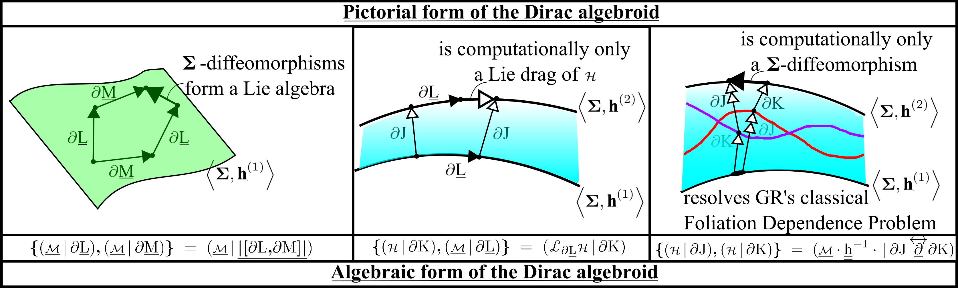
Figure 3: TRi-dressed Dirac algebroid of GR constraints’ a) geometrical significance and b) algebraic structure.

Remark 2 Some further remarks about the Dirac algebroid not yet made in this Series are as follows. It already features in Minkowski spacetime $\mathbb{M}^{n}$ in general coordinates so as to model fleets of accelerated observers therein. This is in fact the context in which Dirac first found this algebroid [5] though he subsequently considered the GR case in [7].

Remark 3 That the Poisson bracket of $\mbox{\scriptsize${\cal C}$}\mbox{hronos}=\mbox{\scriptsize${\cal H}$}$ with itself (43) gives rise to ${\cal S}$huffle constraints $\underline{\mbox{\scriptsize${\cal M}$}}$. This indicates a greater amount of ‘togetherness’ between Temporal and Configurational Relationalism than the RPM model arena exhibits. Consequently, in the GR setting, Temporal Relationalism cannot be entertained without Configurational Relationalism. This is in contrast with how the two can be treated piecemeal in RPM. As an integrability, this is analogous to Thomas precession.

Structure 3 $SO(3,1)$ decomposes under rotations–boosts – $\underline{J}$–$\underline{K}$ split – schematically as

$$\mbox{\bf|[}\underline{J}\mbox{\bf,}\,\underline{J}\mbox{\bf]|}\sim\underline{J}\mbox{ },\mbox{ }\mbox{ }\mbox{\bf|[}\underline{J}\mbox{\bf,}\,\underline{K}\mbox{\bf]|}\sim\underline{K}\mbox{ },\mbox{ }\mbox{ }\mbox{\bf|[}\underline{K}\mbox{\bf,}\,\underline{K}\mbox{\bf]|}\sim\underline{K}+\underline{J}\mbox{ }.$$ (45)

The last bracket is key, since by this the boosts $\underline{K}$ do not constitute a subalgebra. Thomas precession then refers to the rotation arising in this manner from a combination of boosts.

This is of course a spacetime generator matter rather than a constrained one; it is included here, rather, for its analogy with GR’s constraints’ Dirac algebroid.

This is moreover a case in which linearly recombining the two blocks reveals a simpler split form, in accord with the

$$so(3,1)\cong so(3)\times so(3)$$ (46)

accidental relation, as is well-known in both Group Theory and Particle Physics.

This does however amount to abandoning one’s originally declared partition of generators. This partition is of no importance in the current example, but the corresponding partition in the GR case is often considered to be significant.

Structure 4 The GR constraints analogy with Thomas Precession is as follows.

$$\mbox{GR manifests the }\mbox{ }\{\mbox{\scriptsize${\cal H}$}\}\,\,\,\mbox{$\rightarrow$⃝}\,\,\,\{\underline{\mbox{\scriptsize${\cal M}$}}\}\mbox{ }\mbox{ subcase of }\mbox{ }\mbox{\boldmath$\mathfrak{C}$}\mbox{\bf hronos}\,\,\,\mbox{$\rightarrow$⃝}\,\,\,\mbox{ $\mathfrak{G}$}\mbox{\bf auge}\mbox{ }.$$ (47)

So, there is a parallel between composing two boosts producing a rotation: Thomas precession, and composing two time evolutions producing a spatial diffeomorphism: Moncrief–Teitelboim on-slice Lie dragging [14].

Limitation 1 on this analogy is that the GR version takes the form of an algebroid, as required to encode the multiplicity of foliations.

Limitation 2 is that, unlike for Thomas Precession, the integrability cannot be undone by linearly combining constraints.

[There is however a matter time approach supporting redefined constraints that close as a Lie algebra; see Part II of [61] for downsides to matter time approaches however.]

Remark 4 Aside from minisuperspace’s collapse to an Abelian Lie algebra (III.56), other simpler subcases of note are as follows.

Example 5 Strong Gravity [17] demonstrates [40] a smaller a collapse in which both the integrability and the algebroid nature are lost; this is covered in Article IX

Example 6 In spatial dimension 1 and $\mathbb{S}^{1}$ topological manifold, the Dirac algebroid collapses to a Lie algebra (albeit infinite-$d$) that is well known: the Witt algebra, or, with central extension, the Virasoro algebra [25].

This simplification does not however extend to GR in spatial dimension 2 or higher.

Remark 5 Upon including minimally-coupled matter (including no curvature couplings), one has the Teitelboim split [23] for minimally-coupled matter

$$\mbox{\scriptsize${\cal H}$}=\mbox{\scriptsize${\cal H}$}^{\mbox{\scriptsize g}}+\mbox{\scriptsize${\cal H}$}^{\Psi}\mbox{ },\mbox{ }\mbox{ }$$ (48)

$$\underline{\mbox{\scriptsize${\cal M}$}}=\underline{\mbox{{\boldmath\scriptsize${\cal M}$}}}^{\mbox{\scriptsize g}}+\underline{\mbox{{\boldmath\scriptsize${\cal M}$}}}^{\Psi}\mbox{ }.$$ (49)

Teitelboim [23] moreover showed that gravitational and minimally-coupled matter parts obey the Dirac algebroid separately. This follows from (VI.90), the general form taken by minimally-coupled matter potentials, and (49).

There is no difficulty with extending this approach to Einstein–Maxwell or Einstein–Yang–Mills theories; see [23] for a non-TRi account; for a TRi version, just feed Article VI’s constraints with TRi-smearing into the TRi-Dirac Algorithm.

This immediately extends to scalar Gauge Theories as well. For fermionic gauge theories, one needs to work with beins (or similar), by which frame constraints enter at the secondary level. This does not however change the integrability structure or algebroid nature of the subsequent algebraic structure.

Remark 6 See [52] for a further brief introduction to the Dirac algebroid, and e.g. Appendix V of [61] for a brief introduction to algebroids more generally. [38, 34, 36, 47] are texts containing more detailed accounts on the latter. The Author strongly suspects both the latter and the former to be in the infancy of their developments as academic disciplines.

6 Constraint Closure itself

This is also already-TRi and so carries over from Article III. The same applies to Article III’s discussion of Constraint Closure Problems, which moreover include facet interferences with Temporal and/or Configurational Relationalism.

6.1 Seven Strategies for dealing with Constraint Closure Problems

If a severe form of the Constraint Closure Problem strikes, one may have to entirely abandon the candidate theory’s triple $\langle\mathfrak{T}(\mbox{\Large$\mathfrak{q}$}),\mbox{\Large$\mathfrak{g}$},{\cal S}\rangle$. I.e. the Machian variables, a group acting thereupon and the Jacobi–Synge geometrical action. In some cases, however, modifying one or more of these may suffice to attain consistency. This gives the 2-sided cube of strategies of Fig 4.

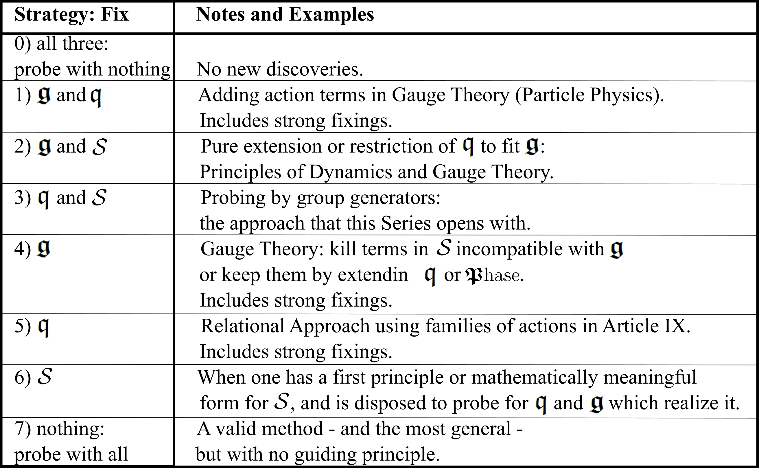
Figure 4: Seven strategies with some capacity for generating new theories from what is allowed by Constraint Closure. In each case, the structures which remain fixed act as a guiding principle. [Keeping a given $\mathfrak{g}$, what physics ensues? What about with a given $\mathfrak{q}$? A given ${\cal S}$?] The unfixed complement structures correspond to types of probing for new theories. Note how this reasoning pitches the Relational Approach as a complementary method to Gauge Theory. Also, paralleling how Gauge Theory can be attempted with extra terms in the action which are then ruled out by lack of $\mathfrak{g}$ compatibility, the current Series’ ‘Relational Approach’ comes in a larger version in which whole families of candidate theories are treated at once (Article IX).

Remark 1 Fig 4’s strategic diversity continues to apply if $\mathfrak{P}$hase and an integrated ($\mbox{\bf d}\partial$A-)Hamiltonian – or its constituent set of constraints in whole-universe theories – are considered in place of $\mathfrak{q}$ and ${\cal S}$. Similar considerations apply in spacetime formulations of ${\cal S}$ with $\mbox{\Large$\mathfrak{g}$}_{\mbox{\scriptsize S}}$ acting thereupon (see Article X) and at the quantum level (further extending the Hamiltonian presentation).

Remark 2 Preserving a particular $\mathfrak{g}$ in Particle Physics includes insisting on a particular internal gauge group, or on the Poincaré group of SR spacetime.

Remark 3 Strong vanishing involves fixing hitherto free constants in ${\cal S}$ so as to avoid the problem.

Remark 4 Among the figure’s three entities, $\mathfrak{q}$ is the one taken to have some tangible physical content. As such, it has the a posteriori right to reject [39, 44, 45] a proposed $\mathfrak{g}$ by triviality or inconsistency.

This role extends to using $\mathfrak{P}$hase instead. One can indeed also consider our eight strategies for the triple

$$\langle\mbox{{\boldmath$\mathfrak{P}$}hase},\mbox{\Large$\mathfrak{g}$},{\cal A}_{\mbox{\bf\tiny${\cal F}$}}\rangle\mbox{ },$$ (50)

where $\mathfrak{g}$ now acts on $\mathfrak{P}$hase and ${\cal A}_{\mbox{\bf\tiny${\cal F}$}}$ is the integrated extended $\mbox{\bf d}\partial$-almost Hamiltonian.

Remark 5) One consequence of adopting strategies permitting extension or reduction of $\mathfrak{q}$ or $\mathfrak{P}$hase is that formulations with second-class constraints are ultimately seen as half-way houses to further formulations which are free thereof. This is largely the context in which both the effective formulation and the Dirac bracket formulation were developed, with $\mathfrak{P}$hase getting extended in the former and reduced in the latter.

Remark 6 With reference to Article III’s classification of Closure Problems, on the one hand whichever of Topological Obstruction, Cascade, Involvement of Specifiers, and Algebraic Interference can be addressed by any of these strategies.

On the other hand, Enforced Group Extension and Enforced Group Reduction require one of strategies 3) or 5-7).

Remark 7 Going full circle, we remind the reader that ‘Cascade’ includes each of relational triviality, triviality, or inconsistency as worst-scenario bounding subcases. We called the last two of these jointly ‘sufficient cascade’, so let us use ‘relationally sufficient cascade’ for the three cases together.

6.2 Further realizations of Constraint Closure Problems

The below examples serve to populate our finer distinctions between types of Constraint Closure phenomena. These examples would however belong more naturally in a longer account of Comparative Background Independence [61, 65, 66, 67], wherein their Configurational and Temporal Relationalism would have already been laid out.

Example 1) [of needing to extend $\mathfrak{g}$] [61]. Correcting one’s action with respect to just the combination of translations $\underline{P}$ and special conformal transformations $\underline{K}$ fails because the ensuing secondary constraints $\underline{\mbox{\boldmath\scriptsize${\cal P}$}}$, $\underline{\mbox{{\boldmath\scriptsize${\cal K}$}}}$ do not form a group without both scaling ${\cal D}$ and rotations $\underline{\mbox{\boldmath\scriptsize${\cal L}$}}$. I.e. schematically,

$$\mbox{\bf\{}\underline{\mbox{\boldmath\scriptsize${\cal P}$}}\mbox{\bf,}\,\underline{\mbox{{\boldmath\scriptsize${\cal K}$}}}\mbox{\bf\}}\mbox{ }\sim\mbox{ }\mbox{\scriptsize${\cal D}$}+\underline{\mbox{\boldmath\scriptsize${\cal L}$}}$$ (51)

This additionally serves as an example of mutual integrabilities.

Example 2) [of failure of $\mathfrak{g}$ to be a gauge group] This is a valid problem in the absence of ${\cal H}$, so attempting to impose $U(1)$ symmetry on Proca Theory suffices. A constraint (24) arises, but this is second-class so it only uses up 1 degree of freedom.

One way out involves considering that Proca Theory rejects quotienting by $U(1)$ (Strategy 3).

Another, if one insists on retaining $U(1)$, is to consider $m=0$ to arise as a strong condition (Strategy 1). This gives a longer route to the exclusion of mass terms from $U(1)$ symmetric 1-form actions.

Proca Theory can indeed be handled with by Dirac brackets or the effective method (Exercise!).

Remark 1 Both of these methods and the preceding strong condition all offer distinct minimalistic ways of dealing with a mismatch in an original candidate triple $\langle\mbox{\Large$\mathfrak{g}$},\mbox{\Large$\mathfrak{q}$},{\cal S}\rangle$.

Example 3) [of abandoning ship due to structural incompatibility] Consider Best Matching with respect to the affine transformations $Aff(d)$ within a Euclidean-norm kinetic arc element [59]. This produces a constraint ${\cal E}$ which is incompatible with $Aff(d)$. This defect can be traced from ${\cal E}$ possessing a Euclidean norm back to the kinetic arc element assumed. In this case, however, progress is not via extension or the Dirac bracket, but rather by acknowledging that one needs to build an arc element free from any residual Euclidean prejudices. Thus one ‘abandons ship’, in the sense of forfeiting a type of ${\cal S}$ for all that one can pass to a different type of working theory [59]. This example’s required alteration so as to attain consistency is however unrelated to changing any of $\mathfrak{g}$, $\mathfrak{q}$ or ${\cal S}$.

Example 4) [Best Matching itself sunk by a Constraint Closure Problem.] Suppose we try to impose a $\mathfrak{g}$ including both the $GL(d,\mathbb{R})$ transformations and the special conformal transformations acting on flat space. Their mutual bracket however forms an obstruction term [59, 61]. This sinking is underlied by Best Matching being just a piecemeal consideration of generators while Constraint Closure involves relations as well as generators.

Example 5) [Mutual second-classness.] We show in Article IX that if the conformogeometrodynamical conditions $\mbox{p}=0$ or $\mbox{p}/\sqrt{\mbox{h}}=$ const are regarded as constraints, they are second-class with respect to ${\cal H}$. An extension strategy for this is outlined in e.g. [63]; on the other hand, the Dirac brackets approach remains untried in this case.

Example 6) [of adjoining new secondary constraints, forcing $\mathfrak{g}$ to be extended via a new integrability arising.] In attempting to set up metrodynamics (no spatial diffeomorphisms presupposed) the Poisson bracket of two ${\cal H}$’s continues to imply a momentum constraint (see Article IX). So ab initio (47) continues to arise [14], giving the claimed extension by integrability. This is furthermore an example of Article II’s point that existence of a natural action of $\mathfrak{g}$ on $\mathfrak{q}$ does not guarantee that $\mathfrak{g}$ represents the totality of physically irrelevant transformations. Our enlargement amounts to being forced to pass from $\mbox{\Large$\mathfrak{g}$}=id$ to the $Diff(\mbox{\boldmath$\Sigma$})$ that corresponds to $\underline{\mbox{{\boldmath\scriptsize${\cal M}$}}}$. This furthermore illustrates that ${\cal C}$hronos can have its own say as to what form (part of) the ${\cal S}$huffle is to take.

Article IX moreover also shows that such a $\mathfrak{g}$-Closure Problem does not however occur in attempting metrodynamical Strong Gravity; this remains consistent with just the one Hamiltonian constraint.

Example 7) Supergravity exemplifies, firstly, ${\cal F}$lin not closing as a subalgebraic structure. This is by the bracket of two linear supersymmetric constraints giving the quadratic Hamiltonian constraint. Since the bracket of two Hamiltonian constraints still returns a linear momentum constraint, moreover, Supergravity also exemplifies two-way integrability

$$\mbox{\boldmath$\mathfrak{F}$}\mbox{\bf lin}\,\,\mbox{$\leftrightarrow$⃝}\,\,\mbox{\boldmath$\mathfrak{C}$}\mbox{\bf hronos}\mbox{ }.$$ (52)

7 Conclusion

Suppose a given theory’s Constraint Closure succeeds as per the current Article.

1) For such as Minisuperspace or Temporally-Relational but Spatially-Absolute Mechanics which do not realize any nontrivial Configurational Relationalism, 1)

$$\mbox{the status of }\mbox{ }{\cal S}^{\mbox{\scriptsize t}\mbox{\scriptsize r}\mbox{\scriptsize i}\mbox{\scriptsize a}\mbox{\scriptsize l}}_{\mbox{\scriptsize T}\mbox{\scriptsize R}\mbox{\scriptsize i}}\mbox{ }\mbox{ can be upgraded to }{\cal S}_{\mbox{\scriptsize C}\mbox{\scriptsize C}-\mbox{\scriptsize T}\mbox{\scriptsize R}\mbox{\scriptsize i}}$$ (53)

ii) The ${\cal C}$hronos arising from this action closes (by itself in these two examples).

iii) This ${\cal C}$hronos can be rearranged to form a Machian emergent time of the conceptual form

$$t^{\mbox{\scriptsize e}\mbox{\scriptsize m}}_{\mbox{\scriptsize C}\mbox{\scriptsize C}\mbox{-}\mbox{\scriptsize R}\mbox{\scriptsize i}}\mbox{ }.$$ (54)

Ri here embraces both Configurational and Temporal Relationalism.

For such as Electromagnetism or Yang–Mills Theory, in each case in flat spacetime viewed canonically, which realizes Configurational Relationalism but not Temporal Relationalism, i)

$$\mbox{the status of }\mbox{ }{\cal S}^{\mbox{\scriptsize t}\mbox{\scriptsize r}\mbox{\scriptsize i}\mbox{\scriptsize a}\mbox{\scriptsize l}}_{\mbox{\scriptsize R}\mbox{\scriptsize e}\mbox{\scriptsize l}}\mbox{ }\mbox{ can be upgraded to }{\cal S}_{\mbox{\scriptsize C}\mbox{\scriptsize C}-\mbox{\scriptsize R}\mbox{\scriptsize i}}$$ (55)

ii) The ${\cal S}$huffle arising from this action closes (by itself in these two examples), constituting moreover not just a ${\cal F}$lin but also a ${\cal G}$auge.

3) For such as RPM or GR-as-Geometrodynamics, which implement both Temporal and Configurational Relationalism, the Relationalism-implementing trial action

$${\cal S}^{\mbox{\scriptsize t}\mbox{\scriptsize r}\mbox{\scriptsize i}\mbox{\scriptsize a}\mbox{\scriptsize l}}_{\mbox{\scriptsize R}\mbox{\scriptsize e}\mbox{\scriptsize l}}\mbox{ }\mbox{ is promoted to }\mbox{ }{\cal S}_{\mbox{\scriptsize C}\mbox{\scriptsize C}-\mbox{\scriptsize R}\mbox{\scriptsize i}}\mbox{ },$$ (56)

ii) Both cases’ ${\cal S}$huffle self-closes and is confirmed to be of not only ${\cal F}$lin but ${\cal G}$auge.

RPM’s $\mbox{\scriptsize${\cal C}$}\mbox{hronos}=\mbox{\scriptsize${\cal E}$}$ also self-closes, whereas GR’s $\mbox{\scriptsize${\cal C}$}\mbox{hronos}=\mbox{\scriptsize${\cal H}$}$ requires GR’s $\mbox{\boldmath\scriptsize${\cal G}$}\mbox{\bf auge}=\underline{\mbox{{\boldmath\scriptsize${\cal M}$}}}$ as an integrability.

The two furthermore mutually-close.

The corresponding Best Matching is now confirmed to have the status

$${\cal S}_{\mbox{\scriptsize C}\mbox{\scriptsize C}\mbox{-}\mbox{\scriptsize R}\mbox{\scriptsize i}}\mbox{ }:=\mbox{ }\mbox{\Large E}_{\mbox{\bf\scriptsize g}\,\in\,\mbox{\large$\mathfrak{g}$}}(\mbox{${\cal S}_{\mbox{\scriptsize C}\mbox{\scriptsize C}\mbox{-}\mbox{\scriptsize R}\mbox{\scriptsize i}}$ built upon $\mbox{\Large$\mathfrak{q}$},\mbox{\Large$\mathfrak{g}$}$})\mbox{ },$$ (57)

where,

$$\mbox{\Large E}_{\mbox{\bf\scriptsize g}\,\in\,\mbox{\large$\mathfrak{g}$}}\mbox{ }=\mbox{ }\{\mbox{extremum over }\mbox{\Large$\mathfrak{g}$}\}\mbox{ }{\cal S}_{\mbox{\scriptsize C}\mbox{\scriptsize C}-\mbox{\scriptsize R}\mbox{\scriptsize i}}$$ (58)

involves a suitable group action of $\mathfrak{g}$, and the whole construct has succeeded in getting past the TRi-Dirac Algorithm.

iii) Finally, these theories’ ${\cal C}$hronos is rearranged to form a Machian emergent time of the conceptual form

$$\mbox{t}^{\mbox{\scriptsize e}\mbox{\scriptsize m}}_{\mbox{\scriptsize C}\mbox{\scriptsize C}\mbox{-}\mbox{\scriptsize R}\mbox{\scriptsize i}}\mbox{ }:=\mbox{ }\mbox{\Large E}^{\prime}_{\mbox{\scriptsize\boldmath$g$}\,\in\,\mbox{\large$\mathfrak{g}$}}\mbox{ }\mbox{t}^{\mbox{\scriptsize e}\mbox{\scriptsize m}}_{\mbox{\scriptsize trial--}\mbox{\large$\mathfrak{g}$}}$$ (59)

for

$$\mbox{t}^{\mbox{\scriptsize e}\mbox{\scriptsize m}}_{\mbox{\scriptsize trial--}\mbox{\large$\mathfrak{g}$}}\mbox{ }:=\mbox{ }\int\frac{||\textrm{d}_{\mbox{\scriptsize\boldmath$g$}}\mbox{\boldmath$Q$}||_{\mbox{\scriptsize\boldmath$M$}}}{\sqrt{2\,W(\mbox{\boldmath$Q$})}}\mbox{ },$$

and where $\mbox{\large E}^{\prime}$ is now likewise protected by ${\cal G}$auge closure.

3)’s full combined implementation of the first three facets of the Problem of Time is summarized in Fig 5. We use here Article I’s colour coding to keep track of single facet contributions and which combinations of facets enter each composite entity involve.

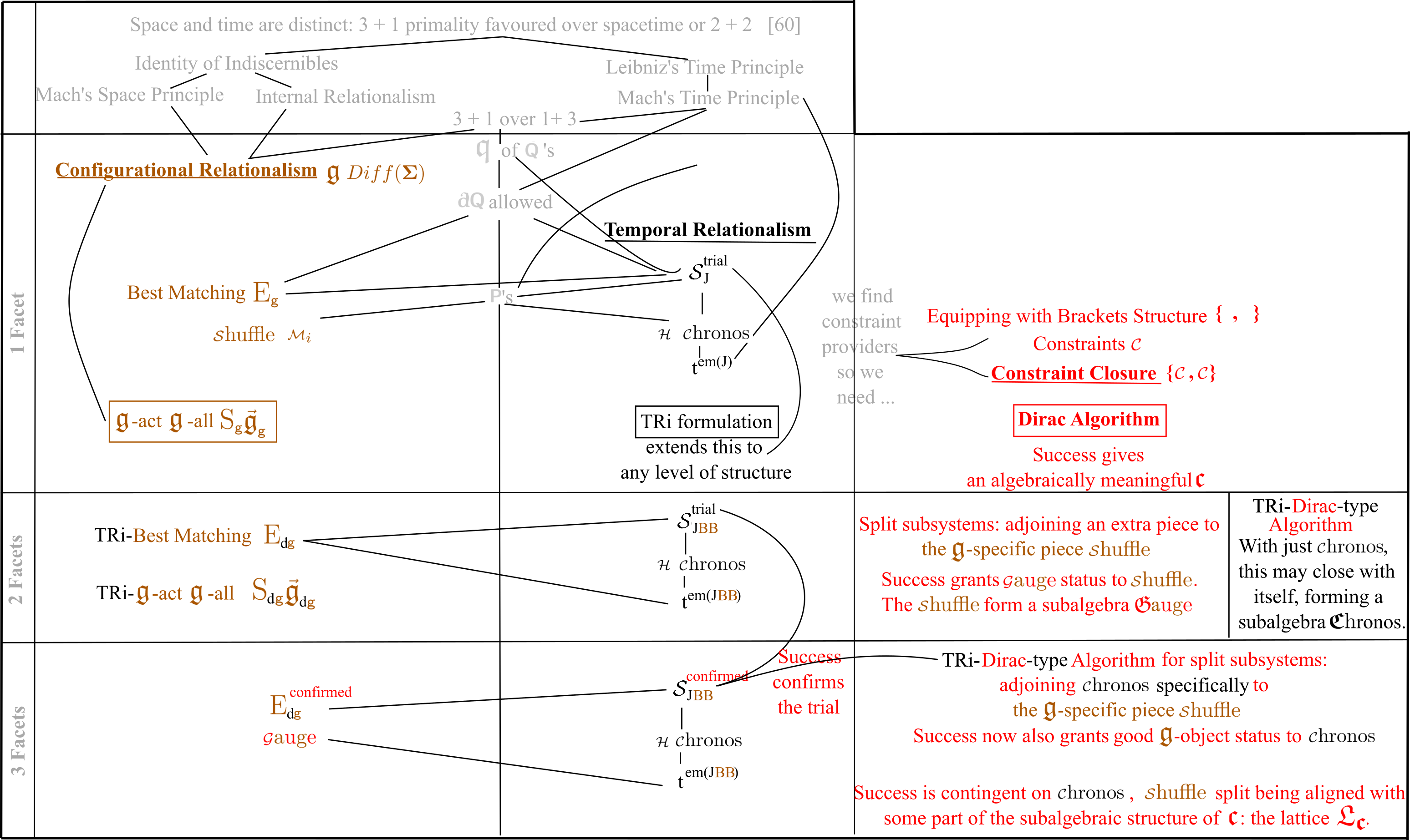
Figure 5: A ‘technicolour guide’ to how the various facet interferences of Constraint Closure (red), Temporal Relationalism (black), and Configurational Relationalism (brown) fit together. This figure can be viewed as an expansion of the leftmost portion of Fig III.6 concerning ‘in which order to address’ Problem of Time facets.

This position reached, each of Assignment of Observables and Spacetime Construction can be considered as separate extensions (Articles VIII and IX respectively). See Article XIII for the overall resolution of the classical local Problem of Time’s facet interference.

Appendix A Supporting Principles of Dynamics developments

A.1 The differential Hamiltonian

TRi requires Hamiltonians to be replaced by differential Hamiltonian [58, 63] change covectors,

$$\mbox{\bf d}\partial{\mathscr{H}}[\mbox{{\bf Q}},\mbox{{\bf P}}]:=\mbox{\bf d}\partial{\mathscr{J}}[\mbox{{\bf Q}},\mbox{\bf d}\partial\mbox{{\bf Q}}]-\mbox{{\bf P}}\,\mbox{\bf d}\partial\mbox{{\bf Q}}\mbox{ }.$$ (60)

These remain rooted however on the same set of Hamiltonian variables, $(\mbox{{\bf Q}},\mbox{{\bf P}})$, these themselves being already-TRi. The differential Hamiltonian thus also lives on $\mathfrak{T}^{*}(\mbox{\Large$\mathfrak{q}$})$.

A.2 Passage to the anti-dRouthian

Structure 1 The current Article also requires passage to the anti-dRouthian [61]

$${\mathscr{A}}[\bar{\mbox{{\bf Q}}},\bar{\mbox{{\bf P}}},\textrm{d}\mbox{{\bf c}}]\mbox{ }:=\mbox{ }{\mathscr{L}}[\bar{\mbox{{\bf Q}}},\textrm{d}\bar{\mbox{{\bf Q}}},\textrm{d}\mbox{{\bf c}}]-\bar{\mbox{{\bf P}}}\cdot\dot{\bar{\mbox{{\bf Q}}}}\mbox{ }.$$ (61)

Remark 1 Like passage to the dRouthian, this still involves treating the cyclic differentials as a separate package, albeit now under the diametrically opposite Legendre transformation. The anti-dRouthian completes the ‘Legendre square’ whose other vertices are ${\mathscr{L}}$, ${\mathscr{H}}$ and ${\mathscr{R}}$: Figure 6.

Remark 2 Like passage to the Routhian, passage to the anti-(d)Routhian turns out to be a useful trick. A minor use is in Sec A.6, whereas the major use is in the next subsection. These uses are moreover specific foundational uses, while Routhian tricks are useful in a concrete problem solving manner.

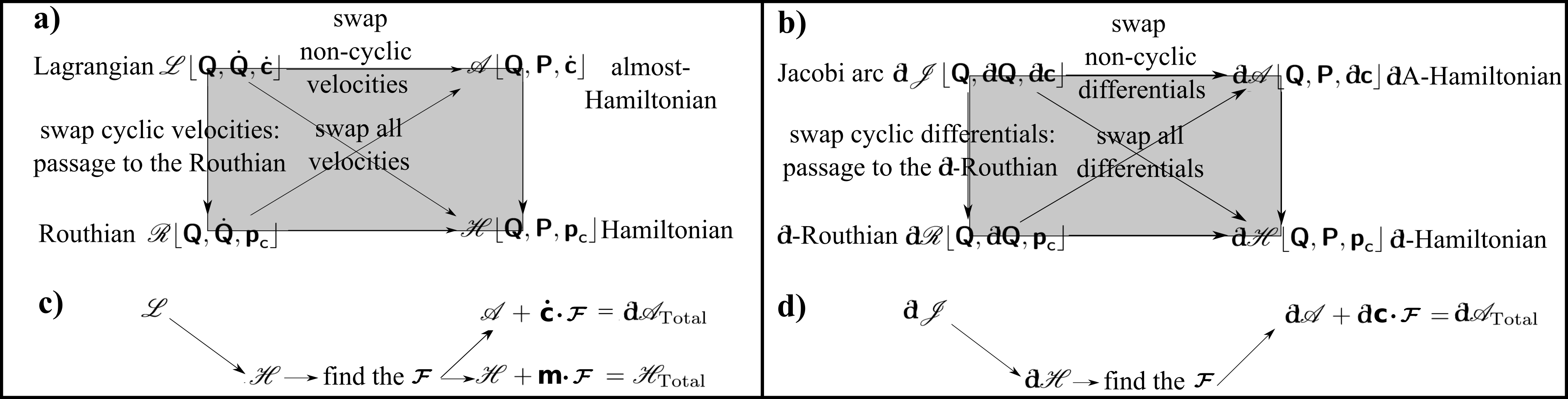
Figure 6: a) Almost-Hamiltonian Legendre square. b) then elevates this square to fully TRi form in terms of d$\partial$-Legendre transformations that dually switch momenta and changes. These are between change covectors: ${\mbox{{\bf\scriptsize d}}\mbox{\scriptsize$\partial$}}{\mathscr{J}}$, ${\mbox{{\bf\scriptsize d}}\mbox{\scriptsize$\partial$}}{\mathscr{R}}$, ${\mbox{{\bf\scriptsize d}}\mbox{\scriptsize$\partial$}}{\mathscr{A}}$, ${\mbox{{\bf\scriptsize d}}\mbox{\scriptsize$\partial$}}{\mathscr{H}}$, the information-preserving extra terms now being subsystem Liouville forms, which were always change covectors. Routhians go to d$\partial$-Routhians; there is no need for ‘almost’ in this case since Routhians are already allowed to contain velocities, and so already include almost-Routhians as a subset. c) and d) exhibit the choices by which the total Hamiltonian, A-Hamiltonian and d$\partial$A-Hamiltonian arise. The starred, primed and extended versions follow suit.

A.3 Further auxiliary spaces

Structure 1 The Lagrangian and Hamiltonian variables respectively form the tangent bundle $\mathfrak{T}(\mbox{\Large$\mathfrak{q}$})$ and cotangent bundle $\mathfrak{T}^{*}(\mbox{\Large$\mathfrak{q}$})$ over $\mathfrak{q}$. From a geometrical perspective, the Legendre transformation for passage to the Hamiltonian is thus a map

$$\mathfrak{T}(\mbox{\Large$\mathfrak{q}$})\longrightarrow\mathfrak{T}^{*}(\mbox{\Large$\mathfrak{q}$})\mbox{ }.$$ (62)

Definition 1 Let $\mathfrak{C}$ be the subconfiguration space of cyclic coordinates and $\check{\mbox{\Large$\mathfrak{q}$}}$ be its complementary subconfiguration space in $\mathfrak{q}$.

Remark 1 The Routhian and the anti-Routhian tricks can now be seen to both come at a price. A first part of this price is geometrical: using these requires the following slightly more complicated mixed cotangent–tangent bundles over $\mathfrak{q}$.

Structure 2

$$\mathfrak{T}(\check{\mbox{\Large$\mathfrak{q}$}})\times\mathfrak{T}^{*}(\mbox{\boldmath$\mathfrak{C}$})$$ (63)

is the bundle space for the Routhian [61], and

$$\mathfrak{T}^{*}(\check{\mbox{\Large$\mathfrak{q}$}})\times\mathfrak{T}(\mbox{\boldmath$\mathfrak{C}$})$$ (64)

is the bundle space for the anti-Routhian [61].

Remark 2 See Appendices A.4-5 for the second and third parts of the price to pay

A.4 Corresponding morphisms

Structure 1 The transformation theory for Hamiltonian variables is more subtle than that of the Lagrangian variables’ $Point$ (already defined in Sec I.2.4). This in part reflects the involvement of

$$\mbox{{\bf P}}\cdot\dot{\mbox{{\bf Q}}}$$ (65)

due to its featuring in the conversion from ${\mathscr{L}}$ to ${\mathscr{H}}$.

1) Starting from $Point$, one can have the momenta follow suit so as to preserve (65) [3]; these transformations indeed preserve ${\mathscr{H}}$.

2) Starting from $Point_{t}$, however, induces gyroscopic corrections to ${\mathscr{H}}$ [3]; this illustrates that ${\mathscr{H}}$ itself can change form.

3) More general transformations which mix the Q and the P are also possible. These are however not as unrestrictedly general functions of their $2\,k$ arguments as $Point$’s transformations are as functions of their $k$ arguments.

3.i) The transformations which preserve the Liouville 1-form

$$\mbox{{\bf P}}\cdot\mbox{\bf d}\partial\mbox{{\bf Q}}\mbox{ },$$ (66)

that is clearly associated with (65). These can again be time-independent (termed scleronomous) or time-dependent in the sense of parametrization adjunction of $t$ to the Q (termed rheonomous). Again, the former preserve $H$ whereas the latter induce correction terms [3]. These are often known as contact transformations, so we denote them by $Contact$ and $Contact_{t}$ respectively.

3.ii) More generally still, preserving the integral of (66) turns out to be useful for many purposes [3]. At the differential level, this corresponds to (66) itself being preserved up to an additive complete differential $\textrm{d}G$ for $G$ the generating function. In this generality, one arrives at the canonical transformations alias symplectomorphisms, once again in the form a rhenonomous group with a scleronomous subgroup. We denote these by $Can_{t}$ and $Can$ respectively; see Fig 7 for how this Sec’s groups fit together to form a lattice of subgroups.

Figure 7: Lattice structure of subgroups of Principles of Dynamics morphisms of varying generality.

Remark 1 Whereas arbitrary canonical transformations do not permit explicit representation, infinitesimal ones do.

Remark 2 Applying Stokes’ Theorem to the integral of (66) reveals a more basic invariant: the bilinear antisymmetric symplectic 2-form [22]

$$\mbox{\bf d}\partial\mbox{{\bf P}}\wedge\mbox{\bf d}\partial\mbox{{\bf Q}}\mbox{ }.$$ (67)

We denote this by

$$\mbox{\boldmath$\omega$}\mbox{ }\mbox{ with components }\mbox{ }\omega_{\mbox{{\scriptsize K}}\mbox{{\scriptsize K}}^{\prime}}$$ (68)

where the K indices run over 1 to $2k$. This subsequently features in bracket structures (see e.g. two Section further down).

Remark 3 Concentrating on the $t$-independent case that is central to this Series of Articles, the morphisms for the Routhian formulation are

$$Point(\check{\mbox{\large$\mathfrak{q}$}})\times Can(\mbox{\boldmath$\mathfrak{C}$})\mbox{ }.$$ (69)

The latter piece is usually ignored due to the $c$ being absent and the $\mbox{\boldmath$p$}^{c}$ being constant.

Structure 1 For the $t$-independent anti-Routhian formulation, the morphisms are

$$Can(\check{\mbox{\large$\mathfrak{q}$}})\times Point(\mbox{\boldmath$\mathfrak{C}$})\mbox{ }.$$ (70)

These more complicated morphisms are the second price to pay in considering Routhian or anti-Routhian formulations.

A.5 Peierls brackets

Structure 1 A brackets structure can in fact already be associated with the Lagrangian tangent bundle formulation: the Peierls bracket [6, 41, 42].

Remark 1 This is more complicated than the Poisson bracket through involving Green’s functions. Its explicit form is not required for this Series.

Remark 2 The third part of the price to pay if one uses a Routhian or anti-Routhian is that the mixed cotangent–tangent bundle nature of the variables requires in general mixed Poisson–Peierls brackets.

A.6 (Anti-)Routhian analogue of the Legendre matrix

The passage to the Hamiltonian is well-known to be affected by whether the Legendre matrix is invertible.

We now consider instead whether passage to the (anti-)Routhian is affected as well [58, 61].

Structure 1 The Legendre matrix for the Routhian is

$$\underline{\underline{\mbox{\boldmath$\Lambda$}}}\mbox{ }:=\mbox{ }\frac{\partial^{2}L}{\mbox{\boldmath$\delta$}\partial\dot{\underline{\mbox{{\bf c}}}}\mbox{\boldmath$\delta$}\partial\dot{\underline{\mbox{{\bf c}}}}}\mbox{ },$$

which is zero by (I.35), so this matrix is an relatively uninteresting albeit entirely obstructive object.

The corresponding expressions for acceleration are similarly entirely free of reference to the cyclic variables.

On the other hand, the Legendre matrix for the anti-Routhian is

$$\underline{\underline{\mbox{\boldmath$\Lambda$}}}\mbox{ }:=\mbox{ }\frac{\partial^{2}L}{\mbox{\boldmath$\delta$}\partial\dot{\underline{\bar{\mbox{{\bf Q}}}}}\mbox{\boldmath$\delta$}\partial\dot{\underline{\bar{\mbox{{\bf Q}}}}}}\mbox{ },$$

which is in general nontrivial.

Remark 1 A theory of primary constraints can be based on this rather than on the usual larger Legendre matrix (I.69).

Remark 2 The smaller anti-Routhian trick is the observation that the acceleration of $\bar{\mbox{{\bf Q}}}$ is unaffected by the cyclic variables. I.e. one can take (I.71) again with index X in place of A since the further terms involving the cyclic variables arising from the chain rule are annihilated by (I.35).

A.7 $\mbox{\bf d}\partial$A-Hamiltonians and phase spaces

Structure 1 The Legendre matrix encoding the non-invertibility of the momentum-velocity relations is now supplanted by the $\mbox{\bf d}\partial^{-1}$-Legendre matrix [58, 61] change vector

$$\mbox{\bf d}\partial^{-1}\underline{\underline{\mbox{\boldmath$\Omega$}}}\mbox{ }:=\mbox{ }\frac{\mbox{\boldmath$\delta$}\partial^{2}\mbox{\bf d}\partial\mbox{J}}{\mbox{\boldmath$\delta$}\partial\,\mbox{\bf d}\partial\underline{\mbox{{\bf Q}}}\mbox{\boldmath$\delta$}\partial\,\mbox{\bf d}\partial\underline{\mbox{{\bf Q}}}}\mbox{ }\left(=\frac{\mbox{\boldmath$\delta$}\partial\underline{\mbox{{\bf P}}}}{\mbox{\boldmath$\delta$}\partial\,\mbox{\bf d}\partial\underline{\mbox{{\bf Q}}}}\right)$$ (71)

which encodes the non-invertibility of the momentum-change relations.

Structure 2 The TRi definition of primary constraint then follows in parallel to how the usual definition of primary constraint follows from the Legendre matrix, with secondary constraint remaining defined by exclusion.

Example 1 Dirac’s argument that Reparametrization Invariance implies at least one primary constraint is now recast as Lemma I.5. The specific form of the primary constraint is, of course, ${\cal C}$hronos.

Remark 1 The next idea in building a TRi version of Dirac’s general treatment of constraints is to append constraints to one’s incipient $\mbox{\bf d}\partial$-Hamiltonian not with Lagrange multipliers – which would break TRi – but rather with cyclic differentials. In this way, a $\mbox{\bf d}\partial$A-Hamiltonian is formed; the ‘A’ here stands for ‘almost’, though the $\mbox{\bf d}\partial$A-Hamiltonian is also a particular case of $\mbox{\bf d}\partial$-anti-Routhian.

The $\mbox{\bf d}\partial$A-Hamiltonian $\mbox{\bf d}\partial A$ symbol aditionally has an extra minus sign relative to the $\mbox{\bf d}\partial$-anti-Routhian $\mbox{\bf d}\partial A$ symbol. This originates from the definition of Hamiltonian involving an overall minus sign where the definitions of Routhian and anti-Routhian have none.

Furthermore, in the current context, all the cyclic coordinates involved have auxiliary status and occur in $\mathfrak{g}$-correction combinations. [In the event of a system possessing physical as well as auxiliary cyclic coordinates, one would use a ‘partial’ rather than ‘complete’ anti-Routhian.]

Structure 3 The equations of motion are now $\mbox{\bf d}\partial$A-Hamilton’s equations [58, 61]

$$\mbox{\bf d}\partial{\mbox{{\bf Q}}}\mbox{ }=\mbox{ }\frac{\mbox{\boldmath$\delta$}\partial\mbox{\bf d}\partial{\mathscr{A}}}{\mbox{\boldmath$\delta$}\partial\,\mbox{{\bf P}}}\mbox{ },\mbox{ }\mbox{ }$$ (72)

$$\mbox{\bf d}\partial{\mbox{{\bf P}}}\mbox{ }=\mbox{ }-\frac{\mbox{\boldmath$\delta$}\partial\mbox{\bf d}\partial{\mathscr{A}}}{\mbox{\boldmath$\delta$}\partial\,\mbox{{\bf Q}}}\mbox{ },$$ (73)

augmented by

$$\frac{\mbox{\boldmath$\delta$}\partial\,\mbox{\bf d}\partial{\mathscr{A}}}{\mbox{\boldmath$\delta$}\partial\,\mbox{\bf d}\partial\mbox{{\bf c}}}\mbox{ }=\mbox{ }0\mbox{ }.$$

Remark 2 Appendix A.6’s comment about using the anti-Routhian’s own Legendre matrix carries over to the $\mbox{\bf d}\partial$-anti-Routhian, and thus also to the further identification of a subcase of this as the $\mbox{\bf d}\partial$A-Hamiltonian.

A.8 TRi-morphisms and brackets. ii)

Remark 1 Suppose there are now cyclic differentials to be kept, or which arise from the TRi-Dirac Algorithm. The corresponding morphisms are now a priori of the mixed type [61]

$$Can(\mathfrak{T}^{*}(\mbox{\Large$\mathfrak{q}$}))\times Point(\mbox{\Large$\mathfrak{g}$})\mbox{ }.$$ (74)

Remark 2 The brackets on these spaces are a priori of the mixed Poisson–Peierls type: Poisson as regards $\mbox{{\bf Q}},\mbox{{\bf P}}$ and Peierls as regards $\mbox{\bf d}\partial\mbox{{\bf g}}$.

Remark 3 (14) implies that, as regards the constraints,

$$Can(\mathfrak{T}^{*}(\mbox{\Large$\mathfrak{q}$}))\times Point(\mbox{\Large$\mathfrak{g}$})$$ (75)

reduces to just $Can(\mathfrak{T}^{*}(\mbox{\Large$\mathfrak{q}$}))$ and the mixed brackets reduce to just Poisson brackets on $\mbox{{\bf Q}},\mbox{{\bf P}}$. The physical part of the $\mbox{\bf d}\partial$A-Hamiltonian’s incipient bracket is just a familiar Poisson bracket. This good fortune follows from the $\mbox{\bf d}\partial$A-Hamiltonian being a type of $\mbox{\bf d}\partial$-anti-Routhian, alongside its non-Hamiltonian variables absenting themselves from the constraints due to the best-matched form of the action.

References

- [1]
- [2] S. Lie and F. Engel, Theory of Transformation Groups Vols 1 to 3 (Teubner, Leipzig 1888-1893).
- [3] C. Lanczos, The Variational Principles of Mechanics (University of Toronto Press, Toronto 1949).
- [4] P.A.M. Dirac, “Forms of Relativistic Dynamics", Rev. Mod. Phys. 21 392 (1949).
- [5] P.A.M. Dirac, “The Hamiltonian Form of Field Dynamics", Canad. J. Math. 3 1 (1951).
- [6] R. Peierls, “The Commutation Laws of Relativistic Field Theory", Proc. R. Soc. Lond. A214 143 (1952).
- [7] P.A.M. Dirac, “The Theory of Gravitation in Hamiltonian Form", Proceedings of the Royal Society of London A 246 333 (1958).
- [8] P.G. Bergmann, “Gauge-Invariant" Variables in General Relativity", Phys. Rev. 124 274 (1961).
- [9] R. Arnowitt, S. Deser and C.W. Misner, “The Dynamics of General Relativity", in Gravitation: An Introduction to Current Research ed. L. Witten (Wiley, New York 1962), arXiv:gr-qc/0405109.
- [10] P.A.M. Dirac, Lectures on Quantum Mechanics (Yeshiva University, New York 1964).
- [11] J.-P. Serre, Lie Algebras and Lie Groups (Benjamin, New York 1965).
- [12] B.S. DeWitt, “Quantum Theory of Gravity. I. The Canonical Theory." Phys. Rev. 160 1113 (1967).
- [13] J.A. Wheeler, in Battelle Rencontres: 1967 Lectures in Mathematics and Physics ed. C. DeWitt and J.A. Wheeler (Benjamin, New York 1968).
- [14] V. Moncrief and C. Teitelboim, “Momentum Constraints as Integrability Conditions for the Hamiltonian Constraint in General Relativity", Phys. Rev. D6 966 (1972).
- [15] C. Teitelboim, “How Commutators of Constraints Reflect Spacetime Structure", Ann. Phys. N.Y. 79 542 (1973).
- [16] J. Śniatycki, “Dirac Brackets in Geometric Dynamics", Ann. Inst. H. Poincaré 20 365 (1974).
- [17] C.J. Isham, “Some Quantum Field Theory Aspects of the Superspace Quantization of General Relativity", Proc. R. Soc. Lond. A351 209 (1976).
- [18] S.A. Hojman, K.V. Kuchař and C. Teitelboim, “Geometrodynamics Regained", Ann. Phys. N.Y. 96 88 (1976).
- [19] K.V. Kuchař, “Geometry of Hyperspace. I.", J. Math. Phys. 17 777 (1976).
- [20] K.V. Kuchař, “Kinematics of Tensor Fields in Hyperspace. II.", J. Math. Phys. 17 792 (1976); “Dynamics of Tensor Fields in Hyperspace. III.", 801; “Geometrodynamics with Tensor Sources IV”, 18 1589 (1977).
- [21] C. Teitelboim, “Supergravity and Square Roots of Constraints", Phys. Rev. Lett. 38 1106 (1977).
- [22] V.I. Arnol’d, Mathematical Methods of Classical Mechanics (Springer, New York 1978).
- [23] C. Teitelboim, “The Hamiltonian Structure of Spacetime", in General Relativity and Gravitation: One Hundred Years after the Birth of Albert Einstein Vol 1 ed. A. Held (Plenum Press, New York 1980).
- [24] K.V. Kuchař, “Canonical Methods of Quantization", in Quantum Gravity 2: a Second Oxford Symposium ed. C.J. Isham, R. Penrose and D.W. Sciama (Clarendon, Oxford 1981).
- [25] P. Goddard, A. Kent, and D. Olive, “Unitary Representations of the Virasoro and Super-Virasoro Algebras", Comm. Math. Phys. 103 105 (1986).
- [26] E. Binz, J. Śniatychi and H. Fischer, Geometry of Classical Fields (Elsevier, Amsterdam 1988).
- [27] K.V. Kuchař, “The Problem of Time in Canonical Quantization", in Conceptual Problems of Quantum Gravity ed. A. Ashtekar and J. Stachel (Birkhäuser, Boston, 1991).
- [28] I.A. Batalin and I.V. Tyutin, “Existence Theorem for the Effective Gauge Algebra in the Generalized Canonical Formalism with Abelian Conversion of Second-Class Constraints", Int. J. Mod. Phys A6 3255 (1991).
- [29] M. Henneaux and C. Teitelboim, Quantization of Gauge Systems (Princeton University Press, Princeton 1992).
- [30] K.V. Kuchař, “Time and Interpretations of Quantum Gravity", in Proceedings of the 4th Canadian Conference on General Relativity and Relativistic Astrophysics ed. G. Kunstatter, D. Vincent and J. Williams (World Scientific, Singapore 1992).
- [31] C.J. Isham, “Canonical Quantum Gravity and the Problem of Time", in Integrable Systems, Quantum Groups and Quantum Field Theories ed. L.A. Ibort and M.A. Rodríguez (Kluwer, Dordrecht 1993), gr-qc/9210011.
- [32] K.V. Kuchař, “Canonical Quantum Gravity", in General Relativity and Gravitation 1992, ed. R.J. Gleiser, C.N. Kozamah and O.M. Moreschi M (Institute of Physics Publishing, Bristol 1993), gr-qc/9304012.
- [33] J.B. Barbour, “The Timelessness of Quantum Gravity. I. The Evidence from the Classical Theory", Class. Quant. Grav. 11 2853 (1994).
- [34] I. Vaisman, Lectures on the Geometry of Poisson Manifolds, (Birkhäuser, Basel 1994).
- [35] P.D. D’Eath, Supersymmetric Quantum Cosmology (Cambridge University Press, Cambridge 1996).
- [36] N.P. Landsman, Mathematical Topics between Classical and Quantum Mechanics (Springer–Verlag, New York 1998).
- [37] K.V. Kuchař, “The Problem of Time in Quantum Geometrodynamics", in The Arguments of Time, ed. J. Butterfield (Oxford University Press, Oxford 1999).
- [38] A. Cannas da Silva and A. Weinstein, Geometric Models for Noncommutative Algebras (American Mathematical Society, Berkeley Mathematics Lecture Notes Series 1999).
- [39] J.B. Barbour, B.Z. Foster and N. ó Murchadha, “Relativity Without Relativity", Class. Quant. Grav. 19 3217 (2002), gr-qc/0012089.
- [40] E. Anderson, “Strong-coupled Relativity without Relativity", Gen. Rel. Grav. 36 255 (2004), gr-qc/0205118.
- [41] G. Esposito, G. Marmo and C. Stornaiolo, “Peierls Brackets in Theoretical Physics", hep-th/0209147.
- [42] B.S. DeWitt, The Global Approach to Quantum Field Theory Vols 1 and 2" (Oxford University Press, New York 2003).
- [43] T. Iwai and H. Yamaoka, “Stratified Reduction of Classical Many-Body Systems with Symmetry", J. Phys. A. Math. Gen 38 2415 (2005).
- [44] E. Anderson, “On the Recovery of Geometrodynamics from Two Different Sets of First Principles", Stud. Hist. Phil. Mod. Phys. 38 15 (2007), gr-qc/0511070.
- [45] E. Anderson, “ Does Relationalism Alone Control Geometrodynamics with Sources?", in Classical and Quantum Gravity Research, ed. M.N. Christiansen and T.K. Rasmussen (Nova, New York 2008), arXiv:0711.0285.
- [46] J.B. Barbour and B.Z. Foster, “Constraints and Gauge Transformations: Dirac’s Theorem is not Always Valid", arXiv:0808.1223.
- [47] A. Gracia-Saz and R.A. Mehta, “Lie Algebroid Structures on Double Vector Bundles and Representation Theory of Lie Algebroids", Adv. Math 223 1236 (2010), arXiv:0810.006.
- [48] J.M. Pons, D.C. Salisbury and K.A. Sundermeyer, “Revisiting Observables in Generally Covariant Theories in the Light of Gauge Fixing Methods", Phys. Rev. D80 084015 (2009), arXiv:0905.4564.
- [49] J.M. Pons, D.C. Salisbury and K.A. Sundermeyer, “Observables in Classical Canonical Gravity: Folklore Demystified", for Proceedings of 1st Mediterranean Conference on Classical and Quantum Gravity, arXiv:1001.2726.
- [50] E. Anderson, in Classical and Quantum Gravity: Theory, Analysis and Applications ed. V.R. Frignanni (Nova, New York 2011), arXiv:1009.2157.
- [51] E. Anderson, “The Problem of Time and Quantum Cosmology in the Relational Particle Mechanics Arena", arXiv:1111.1472.
- [52] M. Bojowald, Canonical Gravity and Applications: Cosmology, Black Holes, and Quantum Gravity (Cambridge University Press, Cambridge 2011).
- [53] E. Anderson, in Annalen der Physik, 524 757 (2012), arXiv:1206.2403.
- [54] C. Laurent-Gengoux, A. Pichereau and P. Vanhaecke, Poisson Structures (Springer-Verlag, Berlin 2013).
- [55] E. Anderson and F. Mercati, “Classical Machian Resolution of the Spacetime Construction Problem", arXiv:1311.6541.
- [56] E. Anderson, “Beables/Observables in Classical and Quantum Gravity", SIGMA 10 092 (2014), arXiv:1312.6073.
- [57] E. Anderson, “Problem of Time and Background Independence: the Individual Facets", arXiv:1409.4117.
- [58] E. Anderson, “TRiPoD (Temporal Relationalism implementing Principles of Dynamics)", arXiv:1501.07822.
- [59] E. Anderson, “Six New Mechanics corresponding to further Shape Theories", Int. J. Mod. Phys. D 25 1650044 (2016), arXiv:1505.00488.
- [60] E. Anderson, “On Types of Observables in Constrained Theories", arXiv:1604.05415.
- [61] E. Anderson, Problem of Time. Quantum Mechanics versus General Relativity, (Springer International 2017) Found. Phys. 190; free access to its extensive Appendices is at https://link.springer.com/content/pdf/bbm
- [62] E. Anderson, “A Local Resolution of the Problem of Time", arXiv:1809.01908.
- [63] F. Mercati Shape Dynamics: Relativity and Relationalism (Oxford University Press, New York 2018).
- [64] E. Anderson, “Geometry from Brackets Consistency", arXiv:1811.00564.
- [65] E. Anderson, “Shape Theories. I. Their Diversity is Killing-Based and thus Nongeneric", arXiv:1811.06516.
- [66] E. Anderson, “Shape Theories II. Compactness Selection Principles", arXiv:1811.06528.
- [67] E. Anderson, “Shape Theory. III. Comparative Theory of Backgound Independence", arXiv:1812.08771.
- [68] E. Anderson, “A Local Resolution of the Problem of Time. I. Introduction and Temporal Relationalism", arXiv 1905.06200.
- [69] E. Anderson, “A Local Resolution of the Problem of Time. II. Configurational Relationalism", arXiv 1905.06206.
- [70] E. Anderson, “A Local Resolution of the Problem of Time. III. The other classical facets piecemeal", arXiv 1905.06212.
- [71] E. Anderson, “A Local Resolution of the Problem of Time. IV. Quantum outline and piecemeal Conclusion", arXiv 1905.06294.
- [72] E. Anderson, “A Local Resolution of the Problem of Time. V. Combining Temporal and Configurational Relationalism for Finite Theories", arXiv:1906.03630.
- [73] E. Anderson, “A Local Resolution of the Problem of Time. VI. Combining Temporal and Configurational Relationalism for Field Theories and GR", arXiv:1906.03635.
- [74] E. Anderson, “A Local Resolution of the Problem of Time. VIII. Expression in Terms of Observables", forthcoming.
- [75] E. Anderson, “A Local Resolution of the Problem of Time. IX. Spacetime Reconstruction", arXiv:1906.03642.
- [76] E. Anderson, “A Local Resolution of the Problem of Time. X. Spacetime Relationalism", forthcoming.
- [77] E. Anderson, “A Local Resolution of the Problem of Time. XI. Slightly Inhomogeneous Cosmology", forthcoming.
- [78] E. Anderson, “A Local Resolution of the Problem of Time. XII. Foliation Independence", forthcoming.
- [79] E. Anderson, “A Local Resolution of the Problem of Time. XIII. Classical combined aspects’ Conclusion", forthcoming.
- [80] E. Anderson, “A Local Resolution of the Problem of Time. XIV. Supporting account of Lie’s Mathematics", forthcoming.
- [81] E. Anderson, forthcoming.