Learning to Predict Novel Noun-Noun Compounds

Abstract

We introduce temporally and contextually-aware models for the novel task of predicting unseen but plausible concepts, as conveyed by noun-noun compounds in a time-stamped corpus. We train compositional models on observed compounds, more specifically the composed distributed representations of their constituents across a time-stamped corpus, while giving it corrupted instances (where head or modifier are replaced by a random constituent) as negative evidence. The model captures generalisations over this data and learns what combinations give rise to plausible compounds and which ones do not. After training, we query the model for the plausibility of automatically generated novel combinations and verify whether the classifications are accurate. For our best model, we find that in around 85% of the cases, the novel compounds generated are attested in previously unseen data. An additional estimated 5% are plausible despite not being attested in the recent corpus, based on judgments from independent human raters.

1 Introduction

Compounding is defined as the process of combining two or more lexemes to form a new concept Bauer (2017). For most compounds in English, the first constituent is the modifier, whereas the second is the head. The head usually determines the class to which the compound belongs, whereas the modifier adds specialisation, e.g apple cake is a type of cake. Compounding is thought of as one of the simplest forms of concept formation as it involves use of elements that are already part of the language and requires little or no morphological changes, particularly in English. From the perspective of language acquisition, Berman (2009) found that children acquired compounding construction skills before the other forms of word formation.

Comparatively little effort has been put into investigating the productive word formation process of compounding computationally. Although compounding is a rather challenging process to model as it involves concepts of compositionality and plausibility along with an intricate blend of semantic and syntactic processes, it is, in our view, one of the best starting points for modeling linguistic creativity. In contrast to relatively more studied topics in linguistics creativity, such as automatic poetry generation Ghazvininejad et al. (2017), aesthetics are not involved. Moreover, compounding is limited to phrase level processes, as it involves a combination of known lexemes.

In general, the creative power of language has been understudied in the field of natural language processing (NLP). The main focus is indeed on processing, as the name suggests. Creative thinking is a cognitive ability that fuels innovation. Therefore, the modelling and understanding of the underlying processes of novel concept creation is relevant. Ultimately, we aim to create tools that enhance people’s ability to interface more creatively with large data sets, to build tools that find inspiration in data.

Our main contributions are the introduction of a new task in NLP that sheds light on the basic mechanisms underlying conceptual creativity; an automatic way of evaluating newly generated language; a temporally-aware neural model that learns what are plausible new conceptual combinations by generalising over attested combinations and corrupted instances thereof.

2 Related Work

The related task of automatic novel compound detection was introduced by Lapata and Lascarides Lapata and Lascarides (2003). Their aim is to distinguish rare noun compounds from rare but nonce noun sequences. The biggest difference between their work and ours is that while they identify existing, albeit rare, and therefore possibly relatively novel compounds in corpora, we predict unseen, and therefore novel compounds, in an absolute sense. Still, the overlap between the tasks makes the work relevant. In their experiments, surface features, such as the frequency of the compound head/modifier, the likelihood of a word as a head/modifier, or the surface-grammatical context surrounding a candidate compound perform almost as well as features that are estimated on the basis of existing taxonomies such as WordNet. Although the semantic features they gathered from WordNet did not do very well, we believe our distributional semantic features are more fine-grained. The simple statistical features that did well in distinguishing rare compounds from nonce terms, would not be suitable in our scenario, where we try to generate novel, plausible compounds. We did however, follow their methodology for the automatic extraction of noun-noun compounds from corpora based on their PoS.

Keller and Lapata (2003) obtain frequencies for unseen bigrams (including noun-noun bigrams) in corpora using Web search engines and show evidence of the reliability of the web counts for natural language processing, also by means of studying the correlation between the web counts and human plausibility judgments. The unseen bigrams are generated in a random fashion from corpus data, as the aim is not to generate plausible combinations, but to overcome data sparseness by providing counts from Web searches.

Ó Séaghdha (2010) uses topic models for selectional preference induction, and evaluates his models on the same data as Keller and Lapata (2003) outperforming previous work. As this work tries to predict the plausibility of unseen combinations, it is more closely related to our work. We are, however, first and foremost interested in the temporal aspect of novel compound creation, and therefore use a time-stamped corpus and temporally-aware models. We also use this time-stamped corpus for evaluation, in addition to human plausibility judgments.

We find a number of works in the related field of cognitive science that focus on predicting human acceptability or plausibility ratings with compositional distributional models. Vecchi et al. (2017) focus on novel adjective noun-phrases. They show that the extent to which an adjective alters the distributional representation of a noun it modifies is the most significant factor in determining the acceptability of the phrase. Günther and Marelli (2016) are also concerned with predicting plausibility ratings, but focus on noun-noun compounds instead. The main difference between their work and ours is the fact that our systems are partly neural and use slightly different features, and aim to generate novel, plausible compounds that are evaluated by checking for their existence in a future corpus, whereas they check for correlation with human plausibility ratings on a set of attested and corrupted compounds. However, their careful investigation of the different distributional semantic factors in their model have been very insightful for us and they inspired one of our systems. For example, they found that a higher relatedness between head and compound is associated with higher plausibility. And the similarity between the constituents is associated with a slightly higher plausibility as well. We used these features in one of our models as well.

More recently, Marelli et al. (2017) presented a data-driven computational system for compound semantic processing based on compositional distributional semantics and evaluate the model against behavioral results concerning the processing of novel compounds. They find that the phenomena of relational priming and relational dominance are captured by the compositional distributional semantic models (cDSMs), whose predictions pattern nicely with the results from the behavioral experiments. Although this work proves that the cDSM is psychologically real when it comes to processing novel compounds, and we find inspiration in the architecture of their model, their work is mainly aimed at modelling compound processing, whereas we are focusing on compound prediction.

For the architecture of our model, we were mainly inspired by Van de Cruys Van de Cruys (2014). The problem we are focusing on has many similarities with the task that their paper focuses on: predicting selectional preferences for unseen data. We adopted the architecture of the neural network from this paper as well as the method to generate negative data for training purposes, originally proposed by Collobert and Weston (2008). Apart from the difference in the task we are trying to address, the main differences between their work and ours is the fact that we are adding a temporal aspect to the neural networks.

3 Novel Compound Prediction

In this paper, we address the task of novel compound prediction. Three models are created that use count-based distributed word representations of known compound constituents to predict unseen, but plausible compounds.

3.1 Intuitions and evaluation

In particular, we address the task of predicting novel noun-noun (N-N) compounds: compounds consisting of two constituents that are both nouns. Our method is based on the generalisation power of machine learning. We reason that by compressing the space in ways that are in line with distributional patterns found in observed data, estimates for unobserved yet plausible combinations should be close to the estimates gathered from attested examples. For example, if we have seen glass-bottom boats in corpora, but we have never seen the combination glass canoe (a recent invention), we can infer from the similarity between the components of the compounds that a glass canoe could be a plausible compound even though it has never been seen.

Evaluating plausibility prediction models for novel combinations is non-trivial and previous work has relied mainly on human judgments Günther and Marelli (2016). We aim to find an automatic evaluation method to ease parameter optimisation and model comparison. To this end, we use a time-stamped corpus divided into decades. The last decade is used for testing, with the previous decades used for training the models. This allows us to check whether the novel generated compounds are good predictions of compounds that might emerge in the future. Because the future extends beyond the last decade of our corpus, and the results from our automatic evaluation are pessimistic, we ask human judges to rate the plausibility of a sample of automatically generated novel compounds that are not attested in the last decade (see Sections 7 and 9).

3.2 Two Aspects for Compounding

We hypothesise that in order to computationally model the phenomenon of compounding, we need our models to be both contextually-aware and temporally-aware, which we explain in detail in the subsequent section.

3.2.1 The Contextual Aspect

Psycholinguistic research on N-N compounds in Dutch seems to suggest that constituents such as -molen ‘-mill’ in pepermolen ‘peppermill’ are separately stored as abstract combinatorial structures rather than processed on-line and understood on the basis of their independent constituents: molen ‘mill’ De Jong et al. (2002). For English open compounds, a similar effect was found for the right constituent. To test if this phenomenon has an effect in the process of generating novel compounds, we decided to experiment with two types of contextual contexts: CompoundCentric and CompoundAgnostic.

CompoundAgnostic: These are the standard window-based contexts used in vector-based representations of words. We capture the distributional vectors of the words, irrespective of whether lexemes are found as constituents of a compound or as simple standalone words (see Figure 1(b)).

CompoundCentric: To the best of our knowledge, distributional models that are sensitive to the role a lexeme plays in a compound have not been tested before. Here we capture the distributional vectors of words based on their usage as constituents in a compound. So the word mill would have different representations, depending on its role in a compound. In Figure 1(a), we show an example context that mill gets as a head, and an example context it gets as a modifier.

Head context

$\overbracket{The\ red\ \underbrace{pepper}_{\text{Modifier}}}^{context}\underbrace{mill}_{\text{Head}}\overbracket{is\ on\ the\ shelf}^{context}.$

Modifier context

$\overbracket{The\ new}^{context}\underbrace{mill}_{\text{Modifier}}$ $\overbracket{\underbrace{stone}_{\text{Head}}\ has\ started}^{context}.$

(a)

$\overbracket{The\ huge}^{context}\underbrace{mill}_{\text{Word}}\overbracket{is\ at\ the\ lake}^{context}.$

$\overbracket{The\ red\ pepper}^{context}\underbrace{mill}_{\text{Word}}\overbracket{is\ on\ the\ shelf}^{context}.$

$\overbracket{The\ new}^{context}\underbrace{mill}_{\text{Word}}$ $\overbracket{stone\ has\ started}^{context}.$

(b)

Figure 1: Contexts for (1(a)) CompoundCentric and (1(b)) CompoundAgnostic aspects

3.2.2 The Temporal Aspect

Previous works such as Hamilton et al. (2016) have shown that meanings of certain words change over time. The same can be observed for compounds such as melting pot. The meaning of melting pot deviated from its original meaning (”A blast furnace”) to its current meaning, that of a society where people from many different cultures are living together, and assimilating into a cohesive whole. To test if time does impact our task, we envision two settings for our models:

DecadeCentric: In this setting, we emphasise the temporal aspect by collecting counts of individual compounds and their constituents per decade. We reason that knowing about the usage trend of the constituents of a compound might help to predict which constituents will be combined next. For example, if a certain word is trending, you would expect it to crop up in novel combinations.

DecadeAgnostic: To test if our intuition about the temporal aspect indeed holds true, we also collect the counts of the individual compounds and their constituents without any temporal information.

4 System Overview

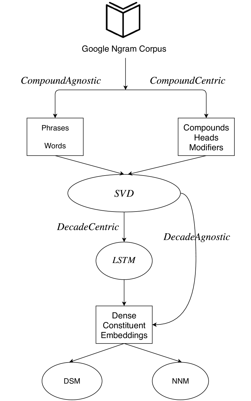
Figure 2: System Overview for the DSM and NNM models

Figure 2 shows the system overview for our two main models. The two aspects explained in the previous section are clearly visible as distinct routes in the system overview. From the Google Ngram Corpus Michel et al. (2010), distributional vectors that are either CompoundAgnostic or CompoundCentric are collected. The counts are either collected per decade (DecadeCentric) or without any temporal information (DecadeAgnostic). The vectors then undergo dimensionality reduction (to 300 dimensions) using singular-value decomposition (SVD), after which they are either directly input to our two semantic models (DecadeAgnostic), or passed through a Long short-term memory (LSTM) model (DecadeCentric) before they are input to the two semantic models. The reason for doing so is that it makes it easier to compare the models for each aspect. The LSTM we use takes a sequence of constituents representations for each decade as input and returns a single representation for the constituent that ideally encompasses its entire history. In the following subsections, we will provide more details on the data processing we performed.

5 Data

We will describe how we collected our data, pre-processed it and how we generated negative data for the classifier.

5.1 Data Collection

We constructed four different datasets based on the aforementioned aspects from the Google Books Ngram corpus Michel et al. (2010). This corpus describes the usage of words and phrases over a period of five centuries. Information of around 6% of all books in eight languages was gathered using Optical Character Recognition (OCR). For our study, we focused on the extraction of English unigrams and bigrams from the corpus and on 20 decades (1800s to 1990s), with the final decade (2000s) only used to collect the newly generated compounds. The corpus was tagged using a Conditional Random Field (CRF) based tagger Lafferty et al. (2001), which has an error rate of 1-5%. The universal PoS tagset Petrov et al. (2011) was used to perform the PoS tagging.

5.2 Data Pre-processing

Similar to Lapata and Lascarides (2003), we made sure that our compounds are not surrounded by nouns, in order to avoid extracting parts of compounds that have more than two constituents. Also, constituents and compounds containing non-alphabetic characters are excluded from the experiments. For each compound and its constituents, a context window of 3 words is used (i.e. 3 words on either side of the target word), in order to retrieve their distributional representations. We were initially limited to a 2-word context window size due to the nature of the Google Ngram 5-gram corpus. However with the use of a sliding window approach, this was increased to a window size of 3. A bigram (say the compound water cycle) could occur in four different positions in the 5-grams (1-2, 2-3, 3-4 and finally 4-5). The contexts for each of these positions is then captured.

We only consider the top 50k most commonly occurring nouns, adjectives, verbs and adverbs to be candidate contexts. Finally, the heads are lemmatised and converted to lowercase. A compound is considered to be novel if it only exists in the final decade (the 2000s) and has a frequency count of at least 3. We chose the cut off count of 3, so as to capture most rare and plausible compounds but at the same time eliminate hapax legomena (terms that occur only once).

5.3 Negative Data Generation

In order to train the classifiers for the task of predicting plausible novel compounds, we need both positive and negative data. The positive class for validation and testing is comprised of the modifier and head of compounds that were newly created in the decades 1990s and 2000s, respectively. In the absence of an attested negative class, i.e. compounds that are implausible, we used the strategy from Collobert and Weston (2008) to generate our own negative class. This class is made up of corrupt tuples, that are constructed by randomly replacing one of the constituents in the tuple ($m$,$h$) with a corresponding constituent (heads are replaced by heads and modifiers by modifiers) from another attested compound.

We then have two scenarios: the CorruptHead and the CorruptModifier scenarios. For a CorruptHead scenario, the head $h$ is replaced by randomly selected head $h^{\prime}$ with the modifier remaining the same. Similarly, for a CorruptModifier scenario, we replace the modifier $m$ with $m^{\prime}$ (see Table 1).

Disambiguation Task

The models have the task of disambiguating the attested tuples from their corrupted counterparts. The purpose of allowing these two scenarios is to test whether corrupting the head leads to better negative data points, than corrupting the modifier. We also make sure that none of the corrupted tuples from the aforementioned procedures results in the generation of a novel or a previously existing compound.

CorruptHead			Novel Compound			CorruptModifier
$m$	$h^{\prime}$		$m$	$h$		$m^{\prime}$	$h$
water	fox		water	absorption		blanket	absorption
pitch	minister	$\leftarrow$	pitch	accent	$\rightarrow$	cement	accent
gene	psychiatry		gene	sequence		dolphin	sequence

Table 1: Generation of negative examples using the CorruptHead and CorruptModifier scenarios

6 Semantic Models

In Figure 2, we show that the distributional vectors, be they CompoundAgnostic or not and be they DecadeAgnostic or not are fed into two distinct semantic models. Note that at this point the distributional vectors are turned into dense representations. We experimented with one additional model, the Distributional Feature Model (DFM), that uses sparse embeddings for constructing its features. The other two models: the Distributional Semantic Models (DSM) and Neural Network Model (NNM) use dense embeddings.

6.1 Distributional Feature Model

In the DFM, for each compound, distributional semantic features are constructed. The raw frequency counts were used to construct the features as weighting measures such as PPMI worsened the final results. The first three are adopted from Information Theory and commonly used to find collocations between words (for more detail see Manning and Schütze (1999)) -

1. Positive Pointwise Mutual Information PPMI: A variation of the Pointwise Mutual Information (PMI) where the negative PMI values are replaced by 0’s. PPMI is preferred over PMI as it has been shown to outperform PMI on semantic similarity tasks Bullinaria and Levy (2007). The PPMI for a compound $comp$ and its two constituents $m$ and $h$ is defined as

   $$\textit{PPMI}(comp)=max(\log_{2}\frac{P(comp)}{P(m)P(h)},0),$$ (1)

   where $P(comp)$ is the probability of both $m$ and $h$ occurring together (i.e. the compound itself).

2. Log likelihood-ratio LLR: PPMI scores are biased towards rare collocations as they assign rare words with rather high PMI values. To overcome this bias and to incorporate the frequency counts of the constituents, the log likelihood ratio is used as another feature, similar to Lyse and Andersen (2012).

3. Local Mutual Information LMI: It is another metric that tries to overcome the bias of PPMI and does so by comparing the probability of observing $m$ and $h$ (or $comp$) together with the probability of observing the two by chance:

   $$\begin{split}\textit{LMI}(comp)&=P(comp)\cdot\log_{2}\frac{P(comp)}{P(m)P(h)}\\ &=P(comp)\cdot PMI\end{split}$$ (2)

   The three features below relate to the calculation of the similarity between the three components of the compound. The similarity between any two target words is defined by the cosine similarity between their vectors.

4. Similarity between the Compound and its Constituents sim-with-head and sim-with-mod: The similarity between a compound $comp$ and a constituent $c$ is defined as:

   $$cos(\overrightarrow{comp},\overrightarrow{c})=\frac{\overrightarrow{comp}\cdot\overrightarrow{c}}{\|\overrightarrow{comp}\|\|\overrightarrow{c}\|},$$ (3)

   where $\overrightarrow{comp}$ and $\overrightarrow{c}$ are the vector representation of $comp$ and $c$, respectively.

5. Similarity between the Constituents: The similarity between the constituents of a compound is computed as well. Günther and Marelli (2016) and Lynott and Ramscar (2001) have found this score to be useful in discerning plausible compounds. Formally, the similarity between a modifier $mod$ and a head $head$ is defined as:

   $$cos(\overrightarrow{mod},\overrightarrow{head})=\frac{\overrightarrow{mod}\cdot\overrightarrow{head}}{\|\overrightarrow{mod}\|\|\overrightarrow{head}\|},$$ (4)

   where $\overrightarrow{mod}$ and $\overrightarrow{head}$ are the vector representation of $mod$ and $head$, respectively.

Finally to retrieve the features for the constituents, the distributional features of the compounds are averaged. We also collect the standard deviation of each feature, so as to get the best approximation of the distribution of the original values. The 6 constituent features (and 114 for the DecadeCentric aspect as there are 19 decades in training) are then concatenated to represent the compound. So in total, we have 12 features (and 228 for the DecadeCentric aspect) as input to the DFM, which uses the stochastic gradient boosting model (XGBoost, Chen and Guestrin, 2016) to perform the supervised learning. The tree-based models were trained using logistic regression as the loss function. The following parameters were then tuned and set as follows : learning rate = 0.1, maximum tree depth = 3, number of estimators = 100, minimum child weight = 6, sub-sample ratio = 0.5, $\gamma$ = 0, $\alpha$ = 0.05 and $\beta$ = 1.

6.2 Neural Network Model

As shown by Van de Cruys (2014) and Tsubaki et al. (2016), neural networks have been successful in composing a representation of a phrase or sentence. Since we expect our novel compounds to be compositional in nature, i.e. their representation could be derived from their constituents’ representations, a compositional neural network should be able to discriminate between plausible candidate compounds and their nonsensical counterparts.

A candidate compound is represented by its modifier and head:

$$x=[i_{m},j_{h}],$$ (5)

where $i$ and $j$ are the vector representations of the modifier $m$ and head $h$, respectively, and the resultant composed vector $x$ serves as the input to the neural network.The vector $x$ is then the input to the NNM.

The architecture of the NNM is similar to the two-way selectional preferences model from Van der Cruys Van de Cruys (2014) and it comprises of a feed-forward neural network with one hidden layer as shown in Figure 3.

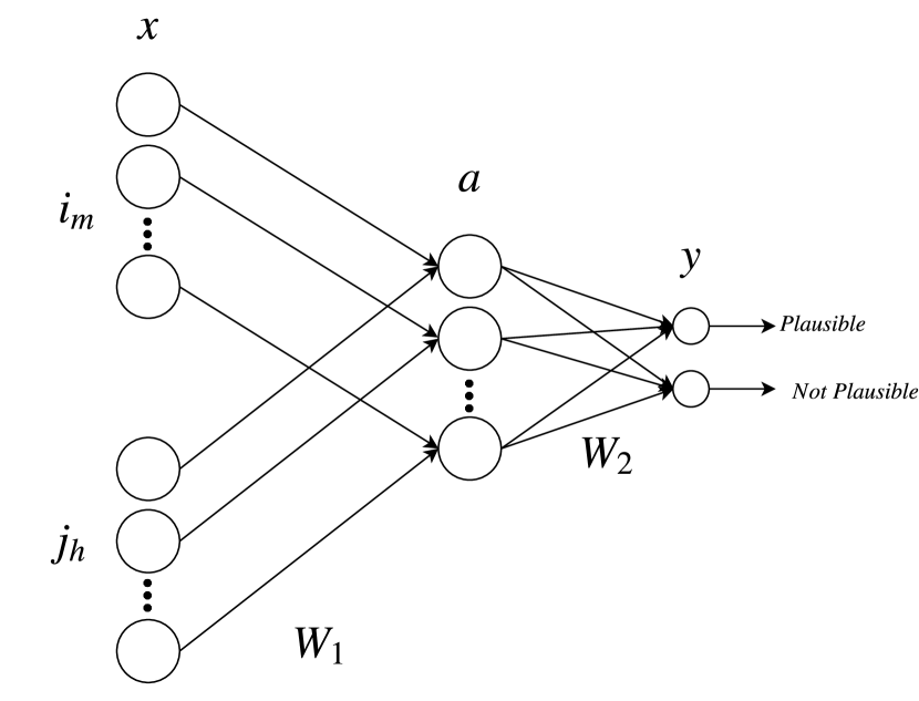
Figure 3: Architecture of NNM

An element-wise activation function rectified linear unit ($ReLU$) is used in the hidden layer:

$$a=f(W_{1}x+b_{1}),$$ (6)

where $a$ is the activation function of the hidden layer with $H$ nodes, $f(.)$ performs an element-wise $ReLU$ function and $W_{1}$ and $b_{1}$ are the weights and bias of the first layer, respectively. In the end, the NNM generates a plausibility score $y$:

$$y=W_{2}~{}a,$$ (7)

where $W_{2}$ is the weight matrix for the final layer. The neural network was trained for 50 epochs with stochastic gradient descent (SGD) used for optimization. A batch size of 100 was chosen and the hidden layer was set to $H=300$ nodes.

6.3 Distributional Semantic Models

In order to discern if a compositional neural network is indeed required for our disambiguation task, we also implement Distributional Semantic Models (DSMs) as a baseline. Since both models (DSMs and NNM) would be using the same constituent embeddings for all four aspects, the final results would help us answer this question. Similar to DFM, we concatenate the constituent features (here embeddings) which are then taken as input to a gradient boosting model, to predict the plausibility.

7 System Evaluation

We evaluate our overall system in two ways: on the basis of corpus data, and by means of human judges, which we cover in Section 9.

For the automatic evaluation of our system, we measure how many of the compounds it predicts are attested among the previously unseen compounds in the last decade, the 2000s. The 18 decades prior to the 1990s (1800s to 1980s) are used to train the models, with the decade 1990s used for validation. The constituents that exist only in the decade of the 2000s are therefore excluded from the training phase. This way we make sure that the prediction of novel entities is dependent only on information derived from the prior decades.

8 Results on Corpus Data

Since all the datasets were equally balanced, we only report the accuracy scores for each of the models. We control the randomness of the negative data generation and run all our semantic models using 10 different datasets. Each of these datasets consists of the same attested novel compounds, along with a different negative class. The results of all the models in our experiments are shown in Table 2.

The NNM produces by far the best results. It attains an accuracy of 85% when the CompoundCentric and DecadeCentric aspects are observed and the heads are corrupted (CorruptHead) in order to generate negative data. This means that for 85% of the compounds generated, the model is able to correctly classify the compound as plausible or implausible. The accuracy in this case is solely determined by the fact that the novel compound is found in the last decade (that is excluded from training). We will show in a separate evaluation (see Section 9) with human judges that this score, although already quite impressive is pessimistic, because some of the novel compounds predicted by the model are not found in the last decade, but still plausible, according to human judges.

Furthermore, the following observations can be made :

Overall, the models that are sensitive to the temporal aspect (DecadeCentric), outperform models that do not take the temporal aspect into account (DecadeAgnostic). This underlines our hypothesis that the temporal aspect is crucial when modelling the process of compounding.

Also, our hypothesis that distributional models should be sensitive to the fact that lexemes as part of a compound differ in meaning from lexemes that appear as standalone words seems to hold true. In general, models that observe the CompoundCentric aspect, perform better. Lastly, corrupting the head to generate negative evidence seems a better alternative than corrupting the modifier. This is to be expected as the head determines most of the compound’s meaning. Replacing the head with another head has a higher probability of generating an implausible compound than replacing the modifier. Implausible compounds are needed to generate negative evidence.

	DecadeCentric
	CompoundCentric		CompoundAgnostic
Model	CorruptHead	CorruptMod	CorruptHead	CorruptMod
DFM	$71.57\pm 0.31$	$68.76\pm 0.2$	$70.95\pm 0.35$	$69.29\pm 0.36$
DSM	$68.18\pm 0.33$	$64.77\pm 0.26$	$67.05\pm 0.71$	$64.03\pm 0.35$
NNM	$84.69\pm 0.33$	$84.55\pm 0.46$	$74.32\pm 0.63$	$76.48\pm 0.56$
	DecadeAgnostic
	CompoundCentric		CompoundAgnostic
Model	CorruptHead	CorruptMod	CorruptHead	CorruptMod
DFM	$69.17\pm 0.24$	$66.69\pm 0.25$	$69.67\pm 0.39$	$67.33\pm 0.27$
DSM	$68.26\pm 0.43$	$65.04\pm 0.34$	$67.52\pm 0.58$	$65.04\pm 0.34$
NNM	$82.92\pm 0.2$	$82.54\pm 0.4$	$72.38\pm 0.92$	$75.02\pm 0.57$

Table 2: Results of the Semantic Models, represented with accuracy and the standard deviation

Compound	Plausibility rating
Service ramp	4
Art direction	3.34
Resource companion	2
Funeral fish	0

Table 3: Human evaluations (average plausibility ratings) for compounds that are non-attested in corpus

9 Human Evaluation

Evaluation on corpus data does not guarantee full coverage. In other words, if a novel compound generated by the system is not found in the contemporary corpus this does not mean per se that the compound is not plausible. The compound might be plausible but not yet ’invented’. We therefore also ran a small-scale manual annotation.

Taking our best model, which was NNM under CompoundCentric and DecadeCentric aspects, a subset of plausible compounds that were predicted by our system (but not found in test corpus and hence counted as incorrect) were annotated by human judges. Following the annotation guidelines of Graves et al. (2013), each annotator was asked to rate each candidate compound between 0 (makes no sense) and 4 (makes complete sense). 250 plausible compounds were annotated in total.

Each candidate compound was evaluated by at least three annotaters. Table 3 shows some of the annotation results. We see that compounds such as art direction and service ramp, that are predicted by the system, but not found in the decades 2000s, is deemed plausible by the annotators. In fact, we found that around $5\%$ of the test data set was rated 3 or higher, on average, by the annotators, indicating that we cannot just rely on a corpora for the evaluation of the novel compound predictor, and that the accuracies given in Table 2 are pessimistic.

10 Conclusions and Future Work

We propose a method for the task of novel compound prediction. We show that this task can be modeled computationally, and that our models need to be both temporally and contextually aware, in order to properly model compounding. The evaluation method we proposed that uses a contemporary corpus to evaluate the novel compound predicted, provides an objective and cheap alternative to evaluation with human judges. In a separate evaluation, we show that the latter provide more optimistic results.

Although previous work has shown correlations between human plausibility judgments on unseen bigrams and frequencies in larger corpora Keller and Lapata (2003), we would like to study the correlation between human plausibility judgments and occurrence in the last decade, to rigorously test the viability of the evaluation method. We would also like to take the graded nature of the plausibility judgments into account when evaluating our models.

In addition, we would like to experiment with other models such as cDSMs and other neural network architectures. Our current system uses a rather simple LSTM architecture to encode temporal information into one representation, and prior tests have shown that enhanced neural network architectures such as Schuster and Paliwal (1997) and Raffel and Ellis (2015) that use bidirectional LSTMS and attention-based networks, respectively, are better at encoding this information.

Lastly, we would like to cover a more diverse set of compounds in future work. Our experiments are currently limited to collecting N-N compounds. In subsequent experiments, we aim to add closed compounds and compounds separated by a hyphen, as well as compounds that are composed of other parts of speech, such as adjective-noun compounds.

References

- Bauer (2017) Laurie Bauer. 2017. Compounds and Compounding. Cambridge Studies in Linguistics. Cambridge University Press.
- Berman (2009) Ruth Berman. 2009. Children’s acquisition of compound constructions. In R. Lieber and P. Stekauer, editors, Handbook of Compounding, pages 298–322. Oxford University Press.
- Bullinaria and Levy (2007) John A. Bullinaria and Joseph P. Levy. 2007. Extracting semantic representations from word co-occurrence statistics: A computational study. Behavior Research Methods, 39(3):510–526.
- Chen and Guestrin (2016) Tianqi Chen and Carlos Guestrin. 2016. XGBoost: A scalable tree boosting system. In Proceedings of the 22nd ACM SIGKDD International Conference on Knowledge Discovery and Data Mining, KDD ’16, pages 785–794, New York, NY, USA. ACM.
- Collobert and Weston (2008) Ronan Collobert and Jason Weston. 2008. A unified architecture for natural language processing: Deep neural networks with multitask learning. In Proceedings of the 25th International Conference on Machine Learning, ICML ’08, pages 160–167, New York, NY, USA. ACM.
- Van de Cruys (2014) Tim Van de Cruys. 2014. A neural network approach to selectional preference acquisition. In Proceedings of the 2014 Conference on Empirical Methods in Natural Language Processing, EMNLP 2014, October 25-29, 2014, Doha, Qatar, A meeting of SIGDAT, a Special Interest Group of the ACL, pages 26–35.
- De Jong et al. (2002) Nivja H. De Jong, Laurie B. Feldman, Robert Schreuder, Matthew Pastizzo, and R. Harald Baayen. 2002. The processing and representation of dutch and english compounds: peripheral morphological and central orthographic effects. Brain and Language, 81:555–67.
- Ghazvininejad et al. (2017) Marjan Ghazvininejad, Xing Shi, Jay Priyadarshi, and Kevin Knight. 2017. Hafez: an interactive poetry generation system. In Proceedings of ACL 2017, System Demonstrations, pages 43–48, Vancouver, Canada. Association for Computational Linguistics.
- Graves et al. (2013) William W. Graves, Jeffrey R. Binder, and Mark S. Seidenberg. 2013. Noun–noun combination: Meaningfulness ratings and lexical statistics for 2,160 word pairs. Behavior Research Methods, 45(2):463–469.
- Günther and Marelli (2016) Fritz Günther and Marco Marelli. 2016. Understanding Karma Police: The Perceived Plausibility of Noun Compounds as Predicted by Distributional Models of Semantic Representation. PLoS ONE, 11(10):1–36.
- Hamilton et al. (2016) William L. Hamilton, Jure Leskovec, and Dan Jurafsky. 2016. Diachronic word embeddings reveal statistical laws of semantic change. In Proceedings of the 54th Annual Meeting of the Association for Computational Linguistics (Volume 1: Long Papers), pages 1489–1501. Association for Computational Linguistics.
- Keller and Lapata (2003) Frank Keller and Mirella Lapata. 2003. Using the web to obtain frequencies for unseen bigrams. Coputational Linguistics, 29(3):459–484.
- Lafferty et al. (2001) John D. Lafferty, Andrew McCallum, and Fernando C. N. Pereira. 2001. Conditional random fields: Probabilistic models for segmenting and labeling sequence data. In Proceedings of the Eighteenth International Conference on Machine Learning, ICML ’01, pages 282–289, San Francisco, CA, USA. Morgan Kaufmann Publishers Inc.
- Lapata and Lascarides (2003) Mirella Lapata and Alex Lascarides. 2003. Detecting novel compounds: The role of distributional evidence. In Proceedings of the Tenth Conference on European Chapter of the Association for Computational Linguistics - Volume 1, EACL ’03, pages 235–242, Stroudsburg, PA, USA. Association for Computational Linguistics.
- Lynott and Ramscar (2001) Dermot Lynott and Michael Ramscar. 2001. Can we model conceptual combination using distributional information? In Proceedings of the 12th Irish Conference on Artificial Intelligence and Cognitive Science, pages 1–10.
- Lyse and Andersen (2012) Gunn Inger Lyse and Gisle Andersen. 2012. Collocations and statistical analysis of n-grams: Multiword expressions in newspaper text. Exploring newspaper language: Using the web to create and investigate a large corpus of modern Norwegian,, pages 79–110.
- Manning and Schütze (1999) Christopher D. Manning and Hinrich Schütze. 1999. Foundations of Statistical Natural Language Processing. MIT Press, Cambridge, MA, USA.
- Marelli et al. (2017) Marco Marelli, Christina L. Gagné, and Thomas L. Spalding. 2017. Compounding as Abstract Operation in Semantic Space: Investigating relational effects through a large-scale, data-driven computational model. Cognition, 166:207–224.
- Michel et al. (2010) Jean-Baptiste Michel, Yuan Kui Shen, Aviva Presser Aiden, Adrian Veres, Matthew K. Gray, The Google Books Team, Joseph P. Pickett, Dale Holberg, Dan Clancy, Peter Norvig, Jon Orwant, Steven Pinker, Martin A. Nowak, and Erez Lieberman Aiden. 2010. Quantitative analysis of culture using millions of digitized books. Science.
- Ó Séaghdha (2010) Diarmuid Ó Séaghdha. 2010. Latent variable models of selectional preference. In Proceedings of the 48th Annual Meeting of the Association for Computational Linguistics, pages 435–444, Uppsala, Sweden. Association for Computational Linguistics.
- Petrov et al. (2011) Slav Petrov, Dipanjan Das, and Ryan T. McDonald. 2011. A universal part-of-speech tagset. CoRR, abs/1104.2086.
- Raffel and Ellis (2015) Colin Raffel and Daniel P. W. Ellis. 2015. Feed-forward networks with attention can solve some long-term memory problems. CoRR, abs/1512.08756.
- Schuster and Paliwal (1997) Mike Schuster and Kuldip K. Paliwal. 1997. Bidirectional recurrent neural networks. IEEE Trans. Signal Processing, 45:2673–2681.
- Tsubaki et al. (2016) Masashi Tsubaki, Kevin Duh, Masashi Shimbo, and Yuji Matsumoto. 2016. Non-linear similarity learning for compositionality. In Proceedings of the Thirtieth AAAI Conference on Artificial Intelligence, AAAI’16, pages 2828–2834. AAAI Press.
- Vecchi et al. (2017) Eva Maria Vecchi, Marco Marelli, Roberto Zamparelli, and Marco Baroni. 2017. Spicy adjectives and nominal donkeys: Capturing semantic deviance using compositionality in distributional spaces. Cognitive Science, 41(1):102–136.