Distributed sub-optimal resource allocation via a projected form of singular perturbation

Abstract

Distributed optimization for resource allocation problems is investigated and a sub-optimal continuous-time algorithm is proposed. Our algorithm has lower order dynamics than others to reduce burdens of computation and communication, and is applicable to weight-balanced graphs. Moreover, it can deal with both local set constraints and coupled inequality constraints, and remove the requirement of twice differentiability of the cost function in comparison with the existing sub-optimal algorithm. However, this algorithm is not easy to be analyzed since it involves singular perturbation type dynamics with projected non-differentiable right-hand side. We overcome the encountered difficulties and obtain results including the existence of an equilibrium, the sub-optimality, and the convergence of the algorithm.

, , ,

1 Introduction

[Xiao2006Optimal, Lakshmanan2008Decentralized, Nedic2018Resource, Yuan2018Adaptive, Zhu2019Resource, Xu2019Regularization] [Halabian2019D5G, Bandi2018Robust, Yang2017Distributed, Cherukuri2015Distributed] [Cherukuri2016Initialization, Yi2016Initialization, Yun2019Initialization, Liang2018Distributed] [Kia2017Distributed, Deng2018Distributed, Johansson2008Subgradient, Liang2018Singular, Kokotovic1999Singular]
Recently, distributed multi-agent resource allocation optimization has received much attention from various fields such as control and optimization [Xiao2006Optimal, Lakshmanan2008Decentralized, Nedic2018Resource, Yuan2018Adaptive, Zhu2019Resource, Xu2019Regularization], communication [Halabian2019D5G], management [Bandi2018Robust], and power system [Yang2017Distributed]. Many continuous-time algorithms have been developed to solve these problems. For a brief review, a Laplacian-gradient dynamics has been presented in [Cherukuri2015Distributed], while initialization-free algorithms have been introduced in [Cherukuri2016Initialization, Yi2016Initialization, Yun2019Initialization]. In particular, algorithms given in [Cherukuri2016Initialization, Yi2016Initialization] are based on primal-dual gradient flows, while the algorithm introduced in [Yun2019Initialization] is based on dual gradient. In addition, a distributed algorithm dealing with coupled inequality constraints has been proposed in [Liang2018Distributed] via a modified Lagrangian function.

Network topology is an essential part in distributed algorithm design and analysis. Many distributed algorithms for resource allocation problems rely on undirected graphs, such as [Xiao2006Optimal, Lakshmanan2008Decentralized, Yi2016Initialization, Liang2018Distributed, Yun2019Initialization]. It is well-known that balanced digraphs are less restrictive and more general than undirected graphs. A few works such as [Cherukuri2016Initialization, Kia2017Distributed, Deng2018Distributed] have considered weight-balanced graphs for resource allocation problems, but their methods need additional computation for the spectral information of the Laplacians.

Sub-optimal solution is sometimes preferable because it may simplify algorithm design and reduce the cost of computation. For example, [Johansson2008Subgradient] has developed a simple distributed algorithm to solve an optimal consensus problem and obtained an sub-optimal solution. How can the sub-optimal concept further serve distributed optimization? It is known that distributed algorithms get involved with networks for information sharing, where local “uncoordinated” flows must be compensated for the desired optimality. It becomes much difficult for directed graphs, because an unidirectional flow can only be compensated by others in the network. With these observations, [Liang2018Singular] has presented a simple distributed algorithm for a special resource allocation problem via singular perturbation, which reduces computation and communication burdens and obtains a sub-optimal solution.

In this paper, we propose a projected singular perturbation dynamics for resource allocation problems with local set constraints and coupled inequality constraints. Although the idea originates from [Liang2018Singular], the previous analysis is not applicable to our new algorithm. One reason is that singular perturbation analysis provides first few terms in the Taylor expansion of the trajectory, which requires at least continuous differentiability on the right-hand side of the differential equation [Kokotovic1999Singular]. However, due to the presence of projection in both fast and slow dynamics, the differentiability does not hold. In fact, it is even difficult to ascertain the existence of an equilibrium and its stability and optimality. To overcome these, we employ theories from linear complementarity problems and variational inequalities, and treat the primal and dual parts as two interacted static systems: the former is a perturbed variational inequality problem and the latter is a perturbed complementarity problem. The main contributions of this work are summarized as follows.

1. A distributed singular perturbation type dynamics is developed to solve resource allocation problems with local set constraints and coupled inequality constraints over weight-balanced graphs, whereas [Liang2018Singular] deals with a special problem with coupled equality constraints only.

2. New analysis methods for the equilibrium, sub-optimality and convergence are provided, which deal with a challenging problem involving singular perturbation dynamics with non-differentiable right-hand side. In addition, the assumption on the twice continuous differentiability of the cost function is relaxed.

3. Our algorithm uses local primal and dual variables without any auxiliary variable. Therefore, it has lower order dynamics than those in [Cherukuri2016Initialization, Kia2017Distributed, Deng2018Distributed], and reduces the computation and communication burden.

2 Preliminaries

In this section, we give the basic notations and introduce preliminary knowledge about convex analysis, variational inequalities, and graph theory.

$\mathbb{R}^{n}$ is the $n$-dimensional real vector space and $\mathbb{R}^{n}_{+}$ is the nonnegative orthant. $I_{n}$ is the unit matrix in $\mathbb{R}^{n\times n}$. $\|\cdot\|$ is the Euclidean norm and $\mathbb{B}$ is the unit ball in a Euclidean space. $\otimes$ is the operator of Kroneckor’s product. $col(x_{1},...,x_{n})$ is the column vector stacked with column vectors $x_{1},...,x_{n}$. For a vector $a\in\mathbb{R}^{n}$, $a\leq\bm{0}$ (or $a<\bm{0}$) means that each component of $a$ is less than or equal to zero (or smaller than zero). For vectors $a,b\in\mathbb{R}^{n}$, $a\perp b$ means that $a^{T}b=0$.

For a closed convex set $C$, the projection map $P_{C}:\mathbb{R}^{n}\to C$ is defined as $P_{C}(x)\triangleq\mathop{\operatorname{argmin}}_{y\in C}\|x-y\|$. Two basic properties with respect to the projection operator hold:

$$(x-P_{C}(x))^{T}(P_{C}(x)-y)\geq 0,\quad\forall\,y\in C\text{,}$$ (1)

$$\|P_{C}(x)-P_{C}(y)\|\leq\|x-y\|,\quad\forall\,x,y\in\mathbb{R}^{n}\text{.}$$ (2)

For $x\in C$, the tangent cone to $C$ at $x$ is $\mathcal{T}_{C}(x)\triangleq\{\lim_{k\to\infty}\frac{x_{k}-x}{t_{k}}\,|\,x_{k}\in C,t_{k}>0,\text{ and }x_{k}\to x,t_{k}\to 0\}$, and the normal cone to $C$ at $x$ is $\mathcal{N}_{C}(x)\triangleq\{v\in\mathbb{R}^{n}\,|\,v^{T}(y-x)\leq 0,\text{ for all }y\in C\}$.

A differentiable function $f:C\to\mathbb{R}$ is said to be $\mu$-strongly convex for some constant $\mu\geq 0$ if $(x-y)^{T}(\nabla f(x)-\nabla f(y))\geq\mu\|x-y\|^{2},\,\forall\,x,y\in C$. In other words, $\nabla f$ is $\mu$-strongly monotone.

Given a subset $\Omega\subseteq\mathbb{R}^{n}$ and a map $F:\Omega\to\mathbb{R}^{n}$, the problem of variational inequality, denoted by $\operatorname{VI}(\Omega,F)$, is to find a vector $x\in\Omega$ such that

$$(y-x)^{T}F(x)\geq 0,\quad\forall\,y\in\Omega,$$

and the set of solutions is denoted by $\operatorname{SOL}(\Omega,F)$. When $\Omega$ is closed and convex, the solution of $\operatorname{VI}(\Omega,F)$ can be equivalently reformulated via projection or the normal cone [Facchinei2003Finite]:

$$x\in\operatorname{SOL}(\Omega,F) \Longleftrightarrow\bm{0}=P_{\Omega}(x-F(x))-x$$ (3)

$$\Longleftrightarrow\bm{0}\in F(x)+\mathcal{N}_{\Omega}(x)$$

In particular, if $\Omega=\mathbb{R}^{n}_{+}$ and $F(x)=q+Mx$ for some vector $q\in\mathbb{R}^{n}$ and matrix $M\in\mathbb{R}^{n\times n}$, then the variational inequality becomes so-called linear complementarity problem, denoted by $\operatorname{LCP}(q,M)$, with its solution set denoted by $\operatorname{SOL}(q,M)$.

Consider a network topology described by a weighted graph $\mathcal{G}=\{\mathcal{V},\mathcal{E},\mathcal{A}\}$, where $\mathcal{V}=\{1,2,\ldots N\}$ is the node set, $\mathcal{E}\subseteq\mathcal{V}\times\mathcal{V}$ is the (oriented) edge set, and $\mathcal{A}=[a_{ij}]\in\mathbb{R}^{N\times N}$ is a nonnegative weight matrix. An edge $(j,i)\in\mathcal{E}$ means that node $j$ can send its information to node $i$. In this case, node $j$ is said to be an in-neighbor of node $i$. The set of all in-neighbors of node $i$ is denoted by $\mathcal{N}_{i}$. Also, $a_{ij}>0$ if $j\in\mathcal{N}_{i}$, while $a_{ij}=0$ otherwise. A path is a sequence of vertices connected by edges. $\mathcal{G}$ is said to be strongly connected if there is a path between any pair of vertices. $\mathcal{G}$ is said to be weight-balanced if for every $i\in\mathcal{V}$, $\sum_{j=1}^{N}a_{ij}=\sum_{j=1}^{N}a_{ji}=d_{i}$. The Laplacian matrix of the weight-balanced $\mathcal{G}$ is $L=\mathcal{D}-\mathcal{A}$, where $\mathcal{D}=\operatorname{diag}\{d_{1},...,d_{N}\}\in\mathbb{R}^{N\times N}$. If $\mathcal{G}$ is strongly connected and weight-balanced, then $L+L^{T}$ is positive semidefinite and $0$ is its simple eigenvalue.

3 Formulation and algorithm

In this section, we formulate the distributed resource allocation problem and present our distributed algorithm.

3.1 Problem formulation

Consider a multi-agent network with graph $\mathcal{G}=\{\mathcal{V},\mathcal{E},\mathcal{A}\}$. For each $i\in\mathcal{V}$, the $i$th agent has a decision variable $x_{i}$ in a local feasible set $\Omega_{i}\subset\mathbb{R}^{n_{i}}$. Also, it has a cost function $f_{i}:\Omega\to\mathbb{R}$ and a resource map $g_{i}:\Omega_{i}\to\mathbb{R}^{p}$. Define

$$\bm{x}\triangleq col(x_{1},x_{2},...,x_{N}),\quad\bm{\Omega}\triangleq\Omega_{1}\times\Omega_{2}\times\cdots\times\Omega_{N},\\$$

and the total cost function and resource map

$$f(\bm{x}) \triangleq f_{1}(x_{1})+f_{2}(x_{2})+\cdots+f_{N}(x_{N}),$$

$$g(\bm{x}) \triangleq g_{1}(x_{1})+g_{2}(x_{2})+\cdots+g_{N}(x_{N}).$$

Then the resource allocation problem with coupled inequality constraints can be formulated as

$$\min_{\bm{x}\in\bm{\Omega}}f(\bm{x}),\,\,\text{ s.t. }\,\,g(\bm{x})\leq\bm{0}.$$ (4)

Our goal is to design a distributed algorithm for problem (4) and find some sub-optimal solution. Of course, the design of sub-optimal algorithms should be simpler than those for optimal solutions. We introduce Assumption 1 for the considered distributed optimization problem.

Assumption 1.

• (Objective function) For each $i\in\mathcal{V}$, $f_{i}$ is $\mu_{f}$-strongly convex over $\Omega_{i}$ for some constant $\mu_{f}>0$, and $\nabla f_{i}$ is $\kappa_{f}$-Lipschitz continuous over $\Omega_{i}$ for some $\kappa_{f}>0$.

• (Constraint set and function) For each $i\in\mathcal{V}$, $\Omega_{i}$ is closed and convex, and $g_{i}$ is convex and $\kappa_{g}$-Lipschitz continuous over $\Omega_{i}$ for some constant $\kappa_{g}>0$. Also, $\nabla g_{i}$ is locally Lipschitz continuous over $\Omega_{i}$.

• (Slator’s constraint qualification) There exists a vector $\tilde{\bm{x}}$ that belongs to the relative interior of $\bm{\Omega}$ and satisfies $g(\tilde{\bm{x}})<\bm{0}$.

• (Network topology) Graph $\mathcal{G}$ is strongly connected and weight-balanced.

The convexity of the cost and constraint functions ensures that (4) is a convex optimization problem. The smoothness enables the use of gradient and the constraint qualification ensures first-order necessary conditions. These assumptions are basic and widely used for constrained convex optimizations [Luenberger2016Linear]. The strong connectivity and weight-balance of the network are the same as those in [Cherukuri2016Initialization, Kia2017Distributed, Liang2018Singular, Deng2018Distributed].

3.2 Distributed algorithm

Our algorithm for problem (4) is given as follows.

Algorithm 1 (for each $i\in\mathcal{V}$)

Initialization:

$$x_{i}(0)\in\Omega_{i},\quad\lambda_{i}(0)\in\mathbb{R}_{+}^{p}.$$

Update flows:

$$\left\{\begin{aligned} \dot{x}_{i}&=P_{\Omega_{i}}(x_{i}-\nabla f_{i}(x_{i})-\nabla g_{i}(x_{i})\lambda_{i})-x_{i}\\ \varepsilon\dot{\lambda}_{i}&=\max\big{\{}-\varepsilon\lambda_{i},\,\,\varepsilon g_{i}(x_{i})-\sum_{j\in\mathcal{N}_{i}}a_{ij}(\lambda_{i}-\lambda_{j})\big{\}}\end{aligned}\right.$$ (5)

where $\varepsilon>0$ is a small tunable parameter.

Algorithm 1 is distributed since the update flows of the $i$th agent need only $x_{i}$, $\lambda_{i}$, $\nabla f_{i}(x_{i})$, $\nabla g_{i}(x_{i})$ and the neighbors’ $\lambda_{j}$. The compact form of (5) can be written as

$$\left\{\begin{aligned} \dot{\bm{x}}&=P_{\bm{\Omega}}(\bm{x}-\nabla f(\bm{x})-\bm{v}(\bm{x},\bm{\lambda}))-\bm{x}\\ \varepsilon\dot{\bm{\lambda}}&=P_{\mathbb{R}^{pN}_{+}}(\varepsilon\bm{\lambda}+\varepsilon\bm{u}(\bm{x})-\bm{L}\bm{\lambda})-\varepsilon\bm{\lambda}\end{aligned}\right.$$ (6)

where $\bm{\lambda}\triangleq col(\lambda_{1},...,\lambda_{N})$, $\bm{u}(\bm{x})\triangleq col(g_{1}(x_{1}),...,g_{N}(x_{N}))$, $\bm{v}(\bm{x},\bm{\lambda})\triangleq col(\nabla g_{1}(x_{1})\lambda_{1},...,\nabla g_{N}(x_{N})\lambda_{N})$, $\bm{L}\triangleq L\otimes I_{p}$, and $L$ is the Laplacian matrix.

Remark 1.

The sub-optimal algorithm given in [Liang2018Singular] for coupled equality constraints is

$$\left\{\begin{aligned} \dot{\bm{x}}&=-\nabla f(\bm{x})-\bm{v}(\bm{x},\bm{\lambda})\\ \varepsilon\dot{\bm{\lambda}}&=\varepsilon\bm{u}(\bm{x})-\bm{L}\bm{\lambda}\end{aligned}\right.$$

Our dynamics (6) uses projections to deal with local set constraints and coupled inequalities constraints. Since the projections are not differentiable, some technical difficulties occur in singular perturbation analysis.

Remark 2.

Alternative update flows over undirected graphs, referring to [Yi2016Initialization], can be used as follows.

$$\left\{\begin{aligned} \dot{\bm{x}}&=P_{\bm{\Omega}}(\bm{x}-\nabla f(\bm{x})-\bm{v}(\bm{x},\bm{\lambda}))-\bm{x}\\ \dot{\bm{\lambda}}&=P_{\mathbb{R}^{pN}_{+}}(\bm{\lambda}+\bm{u}(\bm{x})-\bm{L}\bm{\lambda}-\bm{L}\bm{v})-\bm{\lambda}\\ \dot{\bm{v}}&=\bm{L}\bm{\lambda}\end{aligned}\right.$$ (7)

Compared with (7), dynamics (6) does not employ the auxiliary variable $\bm{v}$ so that the computation and communication are simplified.

4 Algorithm analysis

In this section, we analyze the existence of an equilibrium, the sub-optimality, and the convergence.

4.1 Existence

An equilibrium $(\bm{x},\bm{\lambda})$ of Algorithm 1 is a solution to

$$\bm{0} =P_{\bm{\Omega}}(\bm{x}-\nabla f(\bm{x})-\bm{v}(\bm{x},\bm{\lambda}))-\bm{x}$$ (8a)

$$\bm{0} =P_{\mathbb{R}^{pN}_{+}}(\varepsilon\bm{\lambda}+\varepsilon\bm{u}(\bm{x})-\bm{L}\bm{\lambda})-\varepsilon\bm{\lambda}$$ (8b)

which involves projections and nonlinear maps. To show the existence, we first consider the following auxiliary equations

$$\bm{0} =P_{\bm{\mathcal{X}}}(\bm{x}-\nabla f(\bm{x})-\bm{v}(\bm{x},\bm{\lambda}))-\bm{x}$$ (9a)

$$\bm{0} =P_{\mathbb{R}^{pN}_{+}}(\varepsilon\bm{\lambda}+\varepsilon\bm{u}(\bm{x})-\bm{L}\bm{\lambda})-\varepsilon\bm{\lambda}$$ (9b)

where

$$\bm{\mathcal{X}}\triangleq\{\bm{x}\in\bm{\Omega}\,|\,g(\bm{x})\leq\bm{0}\}.$$ (10)

By (3), $\bm{x}$ satisfies (9a) if and only if it is a solution to $\operatorname{VI}(\bm{\mathcal{X}},\nabla f(\cdot)+\bm{v}(\cdot,\bm{\lambda}))$, regarding $\bm{\lambda}$ as an external input. Also, $\bm{\lambda}$ is a solution to (9b) if and only if it is a solution to the generalized equation

$$\bm{0}\in\varepsilon\bm{u}(\bm{x})-\bm{L}\bm{\lambda}+\mathcal{N}_{\mathbb{R}_{+}^{pN}}(\varepsilon\bm{\lambda})=\varepsilon\bm{u}(\bm{x})-\bm{L}\bm{\lambda}+\mathcal{N}_{\mathbb{R}_{+}^{pN}}(\bm{\lambda}),$$

which is also equivalent to $\operatorname{LCP}(-\varepsilon\bm{u}(\bm{x}),\bm{L})$, regarding $\bm{x}$ as an external input. In this way, we can interpret (9) as two interacted static subsystems: One is $\operatorname{VI}$, whose input is $\bm{\lambda}$ and output is

$$\bm{x}\in\operatorname{SOL}(\bm{\mathcal{X}},\nabla f(\cdot)+\bm{v}(\cdot,\bm{\lambda}))\triangleq G_{1}(\bm{\lambda}).$$

The other one is $\operatorname{LCP}$, whose input is $\bm{x}$ and output is

$$\bm{\lambda}\in\operatorname{SOL}(-\varepsilon\bm{u}(\bm{x}),\bm{L})\triangleq G_{2}(\bm{x}).$$

The structure between $G_{1}$ and $G_{2}$ is shown in Fig. 1.

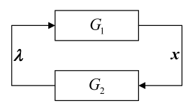
Figure 1: Structure between $G_{1}$ and $G_{2}$.

Consequently, $(\bm{x},\bm{\lambda})$ is a solution to (9) if $\bm{x}\in G_{1}(\bm{\lambda})$ and $\bm{\lambda}\in G_{2}(\bm{x})$, which leads to fixed-point equations

$$\bm{x}\in G_{1}(G_{2}(\bm{x}))\quad\text{and}\quad\bm{\lambda}\in G_{2}(G_{1}(\bm{\lambda})).$$ (11)

Note that $G_{1}$ and $G_{2}$ depend on data of the optimization problem, and $G_{2}$ also depends on the parameter $\varepsilon$.

Lemma 1.

Under Assumption 1, $G_{1}(\bm{\lambda})$ is nonempty and contains only one element for any $\bm{\lambda}\geq\bm{0}$. Moreover,

$$\|G_{1}(\bm{\lambda}^{\prime})-G_{1}(\bm{\lambda})\|\leq\frac{\kappa_{g}}{\mu_{f}}\|\bm{\lambda}^{\prime}-\bm{\lambda}\|,\quad\forall\,\bm{\lambda}^{\prime},\bm{\lambda}\geq\bm{0}.$$

Proof.

The map $\bm{v}(\cdot,\bm{\lambda})$ with $\bm{\lambda}\geq\bm{0}$ is monotone, since

$$(\bm{x}^{\prime}-\bm{x})^{T}(\bm{v}(\bm{x}^{\prime},\bm{\lambda})-\bm{v}(\bm{x},\bm{\lambda}))\\ =\sum_{i=1}^{N}(\bm{x}_{i}^{\prime}-\bm{x}_{i})^{T}(\nabla g_{i}(\bm{x}^{\prime})-\nabla g_{i}(\bm{x}))\bm{\lambda}_{i}\geq 0.$$

Thus, $\nabla f(\cdot)+\bm{v}(\cdot,\bm{\lambda})$ is $\mu_{f}$-strongly monotone. As a result, there exists a unique solution to $\operatorname{VI}(\bm{\mathcal{X}},\nabla f(\cdot)+\bm{v}(\cdot,\bm{\lambda}))$, i.e., $G_{1}(\bm{\lambda})$ is a single-valued map.

Let $\bm{x}^{\prime}=G_{1}(\bm{\lambda}^{\prime})$ and $\bm{x}=G_{1}(\bm{\lambda})$ for any $\bm{\lambda}^{\prime},\bm{\lambda}\geq\bm{0}$. By the definition of variational inequality,

$$(\bm{x}^{\prime}-\bm{x})^{T}(\nabla f(\bm{x})+\bm{v}(\bm{x},\bm{\lambda}))\geq 0,$$

$$(\bm{x}-\bm{x}^{\prime})^{T}(\nabla f(\bm{x}^{\prime})+\bm{v}(\bm{x}^{\prime},\bm{\lambda}^{\prime}))\geq 0.$$

Therefore,

$$(\bm{x}^{\prime}-\bm{x})^{T}(\nabla f(\bm{x}^{\prime})+\bm{v}(\bm{x}^{\prime},\bm{\lambda}^{\prime})-\nabla f(\bm{x})-\bm{v}(\bm{x},\bm{\lambda}))\leq 0.$$

By the strongly convexity of $\nabla f(\cdot)+\bm{v}(\cdot,\bm{\lambda})$,

$$\mu_{f}\|\bm{x}^{\prime}-\bm{x}\|^{2} \leq(\bm{x}^{\prime}-\bm{x})^{T}(\bm{v}(\bm{x}^{\prime},\bm{\lambda})-\bm{v}(\bm{x}^{\prime},\bm{\lambda}^{\prime}))$$

$$\leq\kappa_{g}\|\bm{x}^{\prime}-\bm{x}\|\cdot\|\bm{\lambda}^{\prime}-\bm{\lambda}\|.$$

This completes the proof. ∎

Lemma 2.

Under Assumption 1, the following statements hold:

1. $G_{2}(\bm{x})$ is nonempty for any $\bm{x}\in\bm{\mathcal{X}}$.

2. $G_{2}$ has a unique single-valued continuous selection $G_{2}^{\sharp}$. That is, $G_{2}^{\sharp}$ is a continuous map and $G_{2}^{\sharp}(\bm{x})\in G_{2}(\bm{x})$ for any $\bm{x}\in\bm{\mathcal{X}}$.

3. There is a constant $\kappa_{L}>0$ such that

   $$\|G_{2}^{\sharp}(\bm{x}^{\prime})-G_{2}^{\sharp}(\bm{x})\|\leq\varepsilon\kappa_{g}\kappa_{L}\|\bm{x}^{\prime}-\bm{x}\|,\quad\forall\,\bm{x}^{\prime},\bm{x}\in\bm{\mathcal{X}}.$$

Proof.

Consider $\operatorname{LCP}(-u,L)$, where $L$ is the Laplacian matrix. A point $z\in\operatorname{SOL}(-u,L)$ if and only if

$$z \geq\bm{0}$$ (12a)

$$Lz-u \geq\bm{0}$$ (12b)

$$z^{T}(Lz-u) =0$$ (12c)

$\operatorname{LCP}(-u,L)$ is said to be feasible if there exists a point $z\in\mathbb{R}^{N}$ satisfying (12a) and (12b), not necessarily satisfying (12c). It follows from [Cottle2009Linear, Theorem 3.1.2] that $\operatorname{SOL}(-u,L)$ is nonempty if and only if $\operatorname{LCP}(-u,L)$ is feasible.

Since $L$ has rank $N-1$ and $\bm{1}^{T}L=\bm{0}^{T}$, $\operatorname{LCP}(-u,L)$ is feasible if and only if $u\in U\triangleq\{u\in\mathbb{R}^{N}\,|\,\bm{1}^{T}u\leq 0\}$. Therefore, $S(u)\triangleq\operatorname{SOL}(-u,L)$ is nonempty for $u\in U$, which implies statement 1).

Let $z^{\prime},z\in S(u)$. Then

$$(z^{\prime}-z)^{T}(Lz-u)\geq 0\quad\text{and}\quad(z-z^{\prime})^{T}(Lz^{\prime}-u)\geq 0,$$

which implies

$$(z-z^{\prime})^{T}L(z-z^{\prime})=\frac{1}{2}(z-z^{\prime})^{T}(L+L^{T})(z-z^{\prime})\leq 0.$$

Since $L+L^{T}$ is positive semidefinite, $(L+L^{T})(z-z^{\prime})=0$, which implies $z^{\prime}=z+\bm{1}s$ for some $s\in\mathbb{R}$. Also, it follows from (12c) that $s\bm{1}^{T}u=0$. Thus, $S(u)$ is a singleton for $u\in U^{\circ}\triangleq\{u\in U\,|\,\bm{1}^{T}u<0\}$, and there is a unique selection map $S^{\sharp}(u)\in S(u)$ for $u\in U^{\circ}$. By [Cottle2009Linear, Theorem 7.2.1], there exists a constant $\kappa_{L}>0$ depending on $L$ such that for any $u^{\prime},u\in U$,

$$S(u^{\prime})\subseteq S(u)+\kappa_{L}\|u^{\prime}-u\|\mathbb{B}.$$

Therefore, $S^{\sharp}$ is $\kappa_{L}$-Lipschitz continuous over $U^{\circ}$ and can be extended to $U$ by taking the limit

$$S^{\sharp}(\bar{u})=\lim_{u\to\bar{u},u\in U^{\circ}}S^{\sharp}(u),\quad\forall\,\bar{u}\in U.$$

Thus, statements 2) and 3) hold. ∎

With Lemmas 1 and 2, we present the following theorem.

Theorem 1.

Under Assumption 1, for any $\varepsilon\in(0,\varepsilon^{*})$ with $\varepsilon^{*}\triangleq\frac{\mu_{f}}{\kappa_{g}^{2}\kappa_{L}}$, there exists an equilibrium $(\bm{x}^{*}_{\varepsilon},\bm{\lambda}^{*}_{\varepsilon})$.

Proof.

Since $\varepsilon<\varepsilon^{*}$, there holds a small gain condition

$$\frac{\kappa_{g}}{\mu_{f}}\cdot\varepsilon\kappa_{g}\kappa_{L}<1.$$

Then $G_{1}(G_{2}^{\sharp}(\cdot))$ is a contraction map from $\bm{\mathcal{X}}$ to $\bm{\mathcal{X}}$ and $G_{2}^{\sharp}(G_{1}(\cdot))$ is a contraction map from $\mathbb{R}^{pN}_{+}$ to $\mathbb{R}^{pN}_{+}$. Thus, there exists $(\bm{x}_{\varepsilon}^{\dagger},\bm{\lambda}_{\varepsilon}^{\dagger})\in\bm{\mathcal{X}}\times\mathbb{R}^{pN}_{+}$ as a solution to (9).

Next, we construct a solution to (8). Define

$$f^{\dagger}(\bm{x},\bm{\lambda})\triangleq\sum_{i=1}^{N}f_{i}(x_{i})+\lambda_{i}^{T}g_{i}(x_{i}).$$

Then $\nabla_{\bm{x}}f^{\dagger}(\bm{x},\bm{\lambda})=\nabla f(\bm{x})+\bm{v}(\bm{x},\bm{\lambda})$. By (9), $\bm{x}^{\dagger}_{\varepsilon}$ is the optimal solution to

$$\min_{\bm{x}\in\bm{\Omega}}f^{\dagger}(\bm{x},\bm{\lambda}_{\varepsilon}^{\dagger}),\,\,\text{ s.t. }\,\,g(\bm{x})\leq\bm{0}.$$

Since the Slater’s constraint qualification holds, it follows from Karush-Kuhn-Tucker conditions that there exists a multiplier $\lambda^{\ddagger}\in\mathbb{R}^{p}$ with $\bm{\lambda}^{\ddagger}\triangleq col(\lambda^{\ddagger},...,\lambda^{\ddagger})$ such that

$$\bm{0} \in\nabla f(\bm{x}^{\dagger}_{\varepsilon})+\bm{v}(\bm{x}^{\dagger}_{\varepsilon},\bm{\lambda}^{\dagger}_{\varepsilon}+\bm{\lambda}^{\ddagger})+\mathcal{N}_{\bm{\Omega}}(\bm{x}^{\dagger}_{\varepsilon})$$ (13a)

$$\bm{0} \leq\lambda^{{\ddagger}}\perp-g(\bm{x}^{\dagger}_{\varepsilon})\geq\bm{0}$$ (13b)

Let $(\bm{x}_{\varepsilon}^{*},\bm{\lambda}_{\varepsilon}^{*})\triangleq(\bm{x}^{\dagger}_{\varepsilon},\bm{\lambda}^{\dagger}_{\varepsilon}+\bm{\lambda}^{\ddagger})$. It follows from (13a) that $(\bm{x}_{\varepsilon}^{*},\bm{\lambda}_{\varepsilon}^{*})$ renders (8a). Also, it follows from (9b) and (13b) that $(\bm{x}_{\varepsilon}^{*},\bm{\lambda}_{\varepsilon}^{*})$ renders (8b). In other words, $(\bm{x}_{\varepsilon}^{*},\bm{\lambda}_{\varepsilon}^{*})$ is an equilibrium satisfying (8). This completes the proof. ∎

Remark 3.

We first give a solution to (9) and then a solution to (8), by repeatedly taking advantage of variational inequalities. The method is totally different from that given in [Liang2018Singular]. In addition, $\bm{x}^{*}_{\varepsilon}\in\bm{\mathcal{X}}$ indicates that the solution satisfies the local and coupled constraints in problem (4).

4.2 Sub-optimality

The sub-optimality of Algorithm 1 is as follows.

Theorem 2.

Let $\tilde{\varepsilon}^{*}\triangleq\frac{1}{2}\varepsilon^{*}=\frac{\mu_{f}}{2\kappa_{g}^{2}\kappa_{L}}$ and $K\triangleq\frac{2\kappa_{g}\kappa_{L}\|\bm{u}(\bm{x}^{*})\|}{\mu_{f}}$. Then for any $\varepsilon\in(0,\tilde{\varepsilon}^{*})$, there holds

$$\|\bm{x}^{*}_{\varepsilon}-\bm{x}^{*}\|\leq K\varepsilon.$$ (14)

where $\bm{x}^{*}_{\varepsilon}$ is given in Theorem 1 and $\bm{x}^{*}$ is the optimal solution to problem (4).

Proof.

Since $\bm{x}^{*}$ is the optimal solution to (4), it is also the solution to the variational inequality $\operatorname{VI}(\bm{\mathcal{X}},\nabla f(\cdot))$. That is, $\bm{x}^{*}\in G_{1}(\bm{0})$. Hence,

$$\|\bm{x}_{\varepsilon}^{*}-\bm{x}^{*}\|=\|G_{1}(\bm{\lambda}_{\varepsilon}^{*})-G_{1}(\bm{0})\|\leq\frac{\kappa_{g}}{\mu_{f}}\|\bm{\lambda}_{\varepsilon}^{*}-\bm{0}\|.$$

Since $\bm{\lambda}_{\varepsilon}^{*}\in\operatorname{SOL}(-\varepsilon\bm{u}(\bm{x}_{\varepsilon}^{*}),\bm{L})$ and $\bm{0}\in\operatorname{SOL}(\bm{0},\bm{L})$,

$$\|\bm{\lambda}_{\varepsilon}^{*}-\bm{0}\|\leq\kappa_{L}\|\varepsilon\bm{u}(\bm{x}_{\varepsilon}^{*})-\bm{0}\|.$$

By the $\kappa_{g}$-Lipschitz continuity of $\bm{u}(\cdot)$,

$$\|\bm{u}(\bm{x}_{\varepsilon}^{*})\|\leq\|\bm{u}(\bm{x}^{*})\|+\kappa_{g}\|\bm{x}^{*}_{\varepsilon}-\bm{x}^{*}\|.$$

Therefore,

$$\bigg{(}1-\frac{\kappa_{g}^{2}}{\mu_{f}}\kappa_{L}\varepsilon\bigg{)}\|\bm{x}_{\varepsilon}^{*}-\bm{x}^{*}\|\leq\frac{\kappa_{g}}{\mu_{f}}\kappa_{L}\varepsilon\|\bm{u}(\bm{x}^{*})\|,$$

which implies (14). This completes the proof. ∎

Remark 4.

The expression of $K$ indicates two aspects. First, it shows that the error bound is proportional to $\varepsilon$, since $K$ does not depend on $\varepsilon$. Even the value of $K$ is unknown, one can evaluate that to what extent the accuracy is improved when $\varepsilon$ is reduced. Second, when the Laplacian matrix $L$ is known and the local constrains are bounded, $\kappa_{g},\kappa_{L}$ and the upper bound of $\|\bm{u}(\cdot)\|$ can be estimated offline. In this case, the constant $K$ is available and one can determine the $\varepsilon$ to meet any accuracy of practical use by simple calculation.

4.3 Convergence

The update flows (6) can be written as

$$\dot{\bm{z}}=P_{\bm{\Lambda}}(\bm{z}-\bm{G}(\bm{z}))-\bm{z},$$ (15)

where $\bm{z}\triangleq col(\bm{x},\bm{\lambda}),\bm{\Lambda}\triangleq\bm{\Omega}\times\mathbb{R}_{+}^{pN}$ and

$$\bm{G}(\bm{z})\triangleq\begin{bmatrix}\nabla f(\bm{x})+\bm{v}(\bm{\lambda},\bm{v})\\ \frac{1}{\varepsilon}\bm{L}\bm{\lambda}-\bm{u}(\bm{x})\end{bmatrix}.$$

The map $\bm{G}$ is monotone because

$$(\bm{z}^{\prime}-\bm{z})^{T}(\bm{G}(\bm{z}^{\prime})-\bm{G}(\bm{z}))$$

$$={} {}(\bm{x}^{\prime}-\bm{x})^{T}(\nabla f(\bm{x}^{\prime})-\nabla f(\bm{x})+\bm{v}(\bm{x}^{\prime},\bm{\lambda}^{\prime})-\bm{v}(\bm{x},\bm{\lambda}))$$

$$+(\bm{\lambda}^{\prime}-\bm{\lambda})^{T}(-\bm{u}(\bm{x}^{\prime})+\bm{u}(\bm{x}))+\frac{1}{\varepsilon}(\bm{\lambda}^{\prime}-\bm{\lambda})^{T}\bm{L}(\bm{\lambda}^{\prime}-\bm{\lambda})$$

$$\geq{} {}\mu_{f}\|\bm{x}^{\prime}-\bm{x}\|^{2}+\frac{1}{\varepsilon}(\bm{\lambda}^{\prime}-\bm{\lambda})^{T}\bm{L}(\bm{\lambda}^{\prime}-\bm{\lambda}),\quad\forall\,\bm{z}^{\prime},\bm{z}\in\bm{\Lambda}.$$

In order to obtain the convergence, we employ a Lyapunov candidate function

$$V(\bm{z})\triangleq(\bm{z}-\bm{H}(\bm{z}))^{T}\bm{G}(\bm{z})-\frac{1}{2}\|\bm{z}-\bm{H}(\bm{z})\|^{2}+\frac{1}{2}\|\bm{z}-\bm{z}^{*}\|^{2}\text{,}$$

where $\bm{H}(\bm{z})\triangleq P_{\bm{\Lambda}}(\bm{z}-\bm{G}(\bm{z}))$, and

$$\bm{z}^{*}\in\bm{\Lambda}^{*}\triangleq\{\bm{x}_{\varepsilon}^{*}\}\times\{\bm{\lambda}\,|\,(\bm{x}_{\varepsilon}^{*},\bm{\lambda})\text{ satisfies \eqref{eq:equiAlg}}\}.$$ (16)

Lemma 3.

Under Assumption 1, $V(\bm{z})$ is locally Lipschitz continuous in $\bm{\Lambda}$ and is positive definite with respect to $\bm{z}^{*}$, i.e.,

$$V(\bm{z})\geq 0,\,\forall\,\bm{z}\in\bm{\Lambda}\quad\text{and}\quad V(\bm{z})=0\Leftrightarrow\bm{z}=\bm{z}^{*}.$$

Proof.

By (2), $\bm{H}$ is locally Lipschitz continuous, which indicates that $V$ is also locally Lipschitz continuous. By calculations, $(\bm{z}-\bm{H}(\bm{z}))^{T}\bm{G}(\bm{z})-\frac{1}{2}\|\bm{z}-\bm{H}(\bm{z})\|^{2}=-\frac{1}{2}\|\bm{z}-\bm{G}(\bm{z})-\bm{H}(\bm{z})\|^{2}+\frac{1}{2}\|\bm{G}(\bm{z})\|^{2}=\max_{\bm{y}\in\bm{\Lambda}}\{-\frac{1}{2}\|\bm{z}-\bm{G}(\bm{z})-\bm{y}\|^{2}\}+\frac{1}{2}\|\bm{G}(\bm{z})\|^{2}\geq 0$, where the inequality is obtained by letting $\bm{y}=\bm{z}$. Therefore,

$$V(\bm{z})\geq\frac{1}{2}\|\bm{z}-\bm{z}^{*}\|^{2},\quad\forall\,\bm{z}\in\bm{\Lambda}.$$

This completes the proof. ∎

Lemma 4.

Under Assumption 1, dynamics (15) has a unique trajectory $\bm{z}(t)\in\bm{\Lambda},t\geq 0$. Moreover, the set of equilibria $\bm{\Lambda}^{*}$ given in (16) is Lyapunov stable.

Proof.

Since the right-hand side of (15) is locally Lipschitz continuous, there exists a unique trajectory $\bm{z}(t)$. Also, since $\dot{\bm{z}}\in\mathcal{T}_{\bm{\Lambda}}(\bm{z})$, $\bm{z}(t)\in\bm{\Lambda}$ for all $t\geq 0$.

For the Lyapunov stability of (15), it suffices to prove that $V(\bm{z}(t))$ is non-increasing with respect to $t$. Since $V(\bm{z})$ is locally Lipshcitz continuous and $\bm{z}(t)$ is continuously differentiable, $V(\bm{z}(t))$ is differentiable for almost all $t>0$ with

$$\dot{V}(\bm{z}(t))=\dot{\bm{z}}^{T}(\bm{G}(\bm{z})+\bm{H}(\bm{z})-\bm{z}^{*})\\ -\lim_{\tau\to 0^{+}}\frac{\dot{\bm{z}}^{T}(\bm{G}(\bm{z}+\tau\dot{\bm{z}})-\bm{G}(\bm{z}))}{\tau}.$$

Since $\bm{G}$ is monotone, $\dot{\bm{z}}^{T}(\bm{G}(\bm{z}+\tau\dot{\bm{z}})-\bm{G}(\bm{z}))\geq 0$. Also,

$$\dot{\bm{z}}^{T}(\bm{G}(\bm{z})+\bm{H}(\bm{z})-\bm{z}^{*})=-(W_{1}(\bm{z})+W_{2}(\bm{z})+W_{3}(\bm{z})),$$

where

$$W_{1}(\bm{z}) =(\bm{z}^{*}-\bm{H}(\bm{z}))^{T}(\bm{H}(\bm{z})+\bm{G}(\bm{z})-\bm{z}),$$

$$W_{2}(\bm{z}) =(\bm{z}-\bm{z}^{*})^{T}\bm{G}(\bm{z}^{*}),$$

$$W_{3}(\bm{z}) =(\bm{z}-\bm{z}^{*})^{T}(\bm{G}(\bm{z})-\bm{G}(\bm{z}^{*})).$$

It follows from (1) that $W_{1}(\bm{z})\geq 0$. Moreover, $W_{2}(\bm{z})\geq 0$ because $\bm{z}^{*}$ is a solution to the variational inequality $\operatorname{VI}(\bm{\Lambda},\bm{G})$. Furthermore, $W_{3}(\bm{z})\geq 0$ due to the monotonicity of $\bm{G}$. As a result, $\dot{V}(\bm{z}(t))\leq 0$ for almost all $t>0$. This completes the proof. ∎

The convergence analysis is given in the following result.

Theorem 3.

Under Assumption 1, for any $\varepsilon\in(0,\varepsilon^{*})$, the trajectory of Algorithm 1 converges to an equilibrium point, i.e.,

$$\lim_{t\to\infty}\bm{z}(t)=\tilde{\bm{z}}^{*}\in\bm{\Lambda}^{*},$$ (17)

where $\bm{\Lambda}^{*}$ is given in (16).

Proof.

Since $V(\bm{z}(t))$ is continuous and non-increasing, it follows from the invariance principle that $\bm{z}(t)$ converges to the largest invariant set $\bm{\mathcal{Z}}_{\text{inv}}\subset\bm{\mathcal{Z}}$, where

$$\bm{\mathcal{Z}}\triangleq\{\bm{z}\in\bm{\Lambda}\,|\,(\bm{z}-\bm{z}^{*})^{T}(\bm{G}(\bm{z})-\bm{G}(\bm{z}^{*}))=0,\\ \text{and }(\bm{z}-\bm{z}^{*})^{T}\bm{G}(\bm{z}^{*})=0\}.$$

By the monotonicity of $\bm{G}$, $\bm{z}\in\bm{\mathcal{Z}}$ implies $\bm{x}=\bm{x}^{*}_{\varepsilon}$ and $\bm{L}(\bm{\lambda}-\bm{\lambda}^{*}_{\varepsilon})=\bm{0}$. On the one hand, for $\{\bm{x}^{*}_{\varepsilon}\}$ being invariant, it is necessary that $\dot{\bm{x}}=0$ for any $(\bm{x},\bm{\lambda})\in\bm{\mathcal{Z}}_{\text{inv}}$. Thus, $\bm{\lambda}$ satisfies (8a). On the other hand, it follows from $(\bm{z}-\bm{z}^{*})^{T}\bm{G}(\bm{z}^{*})=0$ that $(\bm{\lambda}-\bm{\lambda}^{*}_{\varepsilon})^{T}(\bm{L}\bm{\lambda}^{*}_{\varepsilon}-\varepsilon\bm{u}(\bm{x}^{*}_{\varepsilon}))=0$. Therefore,

$$\bm{0}\leq\bm{\lambda}\perp\bm{L}\bm{\lambda}-\varepsilon\bm{u}(\bm{x}^{*}_{\varepsilon})\geq\bm{0},$$

which implies that $\bm{\lambda}$ satisfies (9b). Thus, $\bm{\mathcal{Z}}_{\text{inv}}\subset\bm{\Lambda}^{*}$.

Let $\tilde{\bm{z}}^{*}$ be a cluster point of $\bm{z}(t)$ as $t\to+\infty$, i.e., $\tilde{\bm{z}}^{*}$ is a positive limit point of $\bm{z}(t)$. Then $\tilde{\bm{z}}^{*}\in\bm{\mathcal{Z}}_{\text{inv}}$ because the positive limit set is invariant [Khalil2002Nonlinear, Lemma 4.1]. Redefine a Lyapunov function as

$$\tilde{V}(\bm{z})\triangleq(\bm{z}-\bm{H}(\bm{z}))^{T}\bm{G}(\bm{z})-\frac{1}{2}\|\bm{z}-\bm{H}(\bm{z})\|^{2}+\frac{1}{2}\|\bm{z}-\tilde{\bm{z}}^{*}\|^{2}.$$

Since $\tilde{\bm{z}}^{*}\in\bm{\mathcal{Z}}_{\text{inv}}\subset\bm{\Lambda}^{*}$, it follows from similar arguments in Lemmas 3 and 4 that $\tilde{V}$ is non-increasing along the trajectory $\bm{z}(t)$, and meanwhile, $\tilde{V}(\bm{z}(t))\to 0$ as $t\to+\infty$. Thus, the conclusion follows. ∎

Remark 5.

The convergence analysis is based on Lyapunov functions $V$ and $\tilde{V}$. Similar functions have also been considered in [Yi2016Initialization], where a derivative formula for $\nabla V$ is needed with the help of $\nabla^{2}f$. Here, the convergence analysis does not require the twice differentiability of the cost function.

5 Numerical experiments

Table 1: Performance in communication burden, termination time, and relative error of our sub-optimal algorithm and algorithm (7) over different types of graphs with various network sizes. Here, $t_{\text{ter}}=\infty$ means that the algorithm is divergent.

$N$	graph	$d_{\text{mean}}$	$d_{\text{max}}$	algorithm (7)		$\varepsilon=0.1$		$\varepsilon=0.01$		$\varepsilon=0.001$
	type			$t_{\text{ter}}$	$e_{\text{rel}}$	$t_{\text{ter}}$	$e_{\text{rel}}$	$t_{\text{ter}}$	$e_{\text{rel}}$	$t_{\text{ter}}$	$e_{\text{rel}}$
$10$	circle	2	2	$\infty$	-	$12.384$	$7.4768\%$	$12.697$	$0.9062\%$	$12.906$	$0.0929\%$
	random	8	11	$180.108$	$0.0008\%$	$12.615$	$9.0475\%$	$12.686$	$1.1907\%$	$12.9$	$0.1233\%$
	complete	18	18	$31.836$	$0.0003\%$	$12.36$	$3.5692\%$	$12.72$	$0.4063\%$	$12.909$	$0.0419\%$
$50$	circle	2	2	$69.404$	$0.0002\%$	$13.51$	$1.3965\%$	$13.631$	$0.1627\%$	$13.669$	$0.0166\%$
	random	47.96	57	$124.801$	$0.0004\%$	$13.508$	$2.0427\%$	$13.617$	$0.2543\%$	$13.667$	$0.0261\%$
	complete	98	98	$26.597$	$0.0002\%$	$13.543$	$0.8140\%$	$13.651$	$0.0883\%$	$13.671$	$0.009\%$
$100$	circle	2	2	$90.799$	$<0.0001\%$	$13.903$	$1.9957\%$	$14.021$	$0.2295\%$	$14.062$	$0.0233\%$
	random	97.98	112	$705.96$	$0.0006\%$	$13.899$	$4.7095\%$	$13.963$	$0.7167\%$	$14.052$	$0.0759\%$
	complete	198	198	$27.46$	$0.0001\%$	$13.923$	$1.1618\%$	$14.042$	$0.1257\%$	$14.065$	$0.0127\%$
$500$	circle	2	2	$44.782$	$<0.0001\%$	$14.875$	$0.0077\%$	$14.876$	$0.0009\%$	$14.877$	$<0.0001\%$
	random	497.808	542	$1743.164$	$0.0007\%$	$15.127$	$0.0314\%$	$14.875$	$0.0078\%$	$14.876$	$0.0009\%$
	complete	998	998	$20.725$	$<0.0001\%$	$14.875$	$0.0042\%$	$14.88$	$0.0005\%$	$14.877$	$<0.0001\%$
$1000$	circle	2	2	$\infty$	-	$22.572$	$8.8231\%$	$22.185$	$2.5975\%$	$15.01$	$0.6054\%$
	random	998.572	1065	$>2000$	$7.4794\%$	$23.487$	$19.4877\%$	$15.206$	$6.2969\%$	$14.716$	$0.9531\%$
	complete	1998	1998	$53.428$	$<0.0001\%$	$14.65$	$3.0983\%$	$14.987$	$0.3729\%$	$15.21$	$0.0385\%$

Consider a virtualized 5G system consisting of $N$ slices [Halabian2019D5G]. Each slice shares $M$ virtual network functions (VNFs), which are being distributed over $K$ data centers (DCs). Each DC provides resources such as CPU, RAM, bandwidth, and storage. The amount of these $\ell$ types of resources are denoted by vectors $R_{k}\in\mathbb{R}^{\ell},k\in\{1,2,...,K\}$. Also, each slice $i\in\{1,2,...,N\}$ is associated with a set of demand vectors denoted by $d^{k,m}_{i}\in\mathbb{R}^{\ell}$ for each DC $k$ and each VNF $m$. The optimization problem is to determine the amount of resources allocated to each of the VNFs in each DC by minimizing the sum of cost functions of slice thicknesses subjected to resource constraints, i.e.,

$$\begin{array}[]{ll}\mathop{\text{Minimize}}\limits_{\bm{x}}&\sum_{i=1}^{N}f_{i}(x_{i}),\quad f_{i}(x_{i})=\frac{1}{2}(x_{i}-\alpha_{i})^{2}\\ \text{Subject to}&\sum_{i=1}^{N}\sum_{m=1}^{M}x_{i}d^{k,m}_{i}\leq R_{k},\quad k=1,2,...,K\\ &x_{i}\geq 0,\quad i=1,2,...,N\end{array}$$

Set $\ell=K=M=1$ and $N=10,50,100,500,1000$ with directed circles, random digraphs, and complete graphs, respectively. Generate randomly $\alpha_{i}\in[0.5,2],d_{i}^{1,1}\in[0,1],R_{1}\in[0.5N,2N]$ for $i=1,2,...,N$. Set tolerance $\epsilon=10^{-5}$ with the stopping criterion

$$\|\dot{\bm{z}}(t)\|\leq\epsilon,$$

where $\dot{\bm{z}}(t)$ was given in (15). Record the termination time, denoted by $t_{\text{ter}}$, and calculate the relative error

$$e_{\text{rel}}=\frac{\|\bm{x}(t_{\text{ter}})-\bm{x}^{*}\|}{\|\bm{x}^{*}\|}\times 100\%.$$

The instant communication burden of an agent can be characterized by the number of times that it sends and receives information in a unit running time, which equals the sum of its out-degree and in-degree. We record the mean and maximum of such degrees among all agents, denoted by $d_{\text{mean}}$ and $d_{\text{max}}$, respectively. The total amount of communication per agent can be evaluated by using $d_{\text{mean}}\cdot t_{\text{ter}}$ and $d_{\text{max}}\cdot t_{\text{ter}}$ for our algorithm and $2d_{\text{mean}}\cdot t_{\text{ter}}$ and $2d_{\text{max}}\cdot t_{\text{ter}}$ for algorithm (7). Note that these two algorithms do not necessarily share the same termination time $t_{\text{ter}}$, because their convergence speed may be different. In the experiments, the Euler’s method is employed to discretize these algorithms with fixed stepsize $0.001$, and the Laplacian matrices are normalized by scaling the balanced weights such that $\|L\|=1$. Numerical results in Table 1 show that our algorithm achieves acceptable accuracy, fast convergence speed, and significant reduction of computation and communication burden.

6 Conclusions

A distributed continuous-time algorithm has been proposed for resource allocation optimization with local set constraints and coupled inequality constraints over weight-balanced graphs. Existence and sub-optimality of the equilibrium have been established with convergence analysis. Our algorithm and analysis approach have demonstrated the effectiveness of the singular perturbation based sub-optimal design even with non-differentiable right-hand side.

References

• [1] \harvarditem[Bandi et al.]Bandi, Trichakis \harvardand Vayanos2018Bandi2018Robust Bandi, C., Trichakis, N. \harvardand Vayanos, P. \harvardyearleft2018\harvardyearright. Robust multiclass queuing theory for wait time estimation in resource allocation systems, Management Science 65(1): 152–187.
• [2] \harvarditemCherukuri \harvardand Cortés2015Cherukuri2015Distributed Cherukuri, A. \harvardand Cortés, J. \harvardyearleft2015\harvardyearright. Distributed generator coordination for initialization and anytime optimization in economic dispatch, IEEE Transactions on Control of Network Systems 2(3): 226–237.
• [3] \harvarditemCherukuri \harvardand Cortés2016Cherukuri2016Initialization Cherukuri, A. \harvardand Cortés, J. \harvardyearleft2016\harvardyearright. Initialization-free distributed coordination for economic dispatch under varying loads and generator commitment, Automatica 74(12): 183–193.
• [4] \harvarditem[Cottle et al.]Cottle, Pang \harvardand Stone2009Cottle2009Linear Cottle, R. W., Pang, J.-S. \harvardand Stone, R. E. \harvardyearleft2009\harvardyearright. The Linear Complementarity Problem, Vol. 60 of Classics in Applied Mathematics, SIAM, Commonwealth of Pennsylvania.
• [5] \harvarditem[Deng et al.]Deng, Liang \harvardand Hong2018Deng2018Distributed Deng, Z., Liang, S. \harvardand Hong, Y. \harvardyearleft2018\harvardyearright. Distributed continuous-time algorithms for resource allocation problems over weight-balanced digraphs, IEEE Transactions on Cybernetics 48(11): 3116–3125.
• [6] \harvarditemFacchinei \harvardand Pang2003Facchinei2003Finite Facchinei, F. \harvardand Pang, J. \harvardyearleft2003\harvardyearright. Finite-Dimensional Variational Inequalities and Complementarity Problems, Operations Research, Springer-Verlag, New York.
• [7] \harvarditemHalabian2019Halabian2019D5G Halabian, H. \harvardyearleft2019\harvardyearright. Distributed resource allocation optimization in 5G virtualized networks, IEEE Journal on Selected Areas in Communications 37(3): 627–642.
• [8] \harvarditem[Johansson et al.]Johansson, Keviczky, Johansson \harvardand Johansson2008Johansson2008Subgradient Johansson, B., Keviczky, T., Johansson, M. \harvardand Johansson, K. H. \harvardyearleft2008\harvardyearright. Subgradient methods and consensus algorithms for solving convex optimization problems, The 47th IEEE Conference on Decision and Control (CDC), IEEE, Cancun, Mexico, pp. 4185–4190.
• [9] \harvarditemKhalil2002Khalil2002Nonlinear Khalil, H. K. \harvardyearleft2002\harvardyearright. Nonlinear Systems, 3 edn, Prentice Hall, New Jersey.
• [10] \harvarditemKia2017Kia2017Distributed Kia, S. S. \harvardyearleft2017\harvardyearright. Distributed optimal in-network resource allocation algorithm design via a control theoretic approach, Systems & Control Letters 107: 49–57.
• [11] \harvarditem[Kokotovic et al.]Kokotovic, Khalil \harvardand O’reilly1999Kokotovic1999Singular Kokotovic, P., Khalil, H. K. \harvardand O’reilly, J. \harvardyearleft1999\harvardyearright. Singular Perturbation Methods in Control: Analysis and Design, Vol. 25 of Classics in Applied Mathematics, SIAM, Commonwealth of Pennsylvania.
• [12] \harvarditemLakshmanan \harvardand De Farias2008Lakshmanan2008Decentralized Lakshmanan, H. \harvardand De Farias, D. P. \harvardyearleft2008\harvardyearright. Decentralized resource allocation in dynamic networks of agents, SIAM Journal of Optimization 19(2): 911–940.
• [13] \harvarditem[Liang et al.]Liang, Zeng \harvardand Hong2018aLiang2018Distributed Liang, S., Zeng, X. \harvardand Hong, Y. \harvardyearleft2018a\harvardyearright. Distributed nonsmooth optimization with coupled inequality constraints via modified Lagrangian function, IEEE Transactions on Automatic Control 63(6): 1753–1759.
• [14] \harvarditem[Liang et al.]Liang, Zeng \harvardand Hong2018bLiang2018Singular Liang, S., Zeng, X. \harvardand Hong, Y. \harvardyearleft2018b\harvardyearright. Distributed sub-optimal resource allocation over weight-balanced graph via singular perturbation, Automatica 95: 222–228.
• [15] \harvarditemLuenberger \harvardand Ye2016Luenberger2016Linear Luenberger, D. G. \harvardand Ye, Y. \harvardyearleft2016\harvardyearright. Linear and Nonlinear Programming, Vol. 228 of Operations Research & Management Science, Springer-Verlag, New York.
• [16] \harvarditem[Nedić et al.]Nedić, Olshevsky \harvardand Shi2018Nedic2018Resource Nedić, A., Olshevsky, A. \harvardand Shi, W. \harvardyearleft2018\harvardyearright. Improved convergence rates for distributed resource allocation, The 57th IEEE Conference on Decision and Control (CDC), Miami Beach, FL, USA, pp. 172–5458.
• [17] \harvarditemXiao \harvardand Boyd2006Xiao2006Optimal Xiao, L. \harvardand Boyd, S. \harvardyearleft2006\harvardyearright. Optimal scaling of a gradient method for distributed resource allocation, Journal of Optimization Theory and Applications 129(3): 469–488.
• [18] \harvarditem[Xu et al.]Xu, Zhu, Soh \harvardand Xie2019Xu2019Regularization Xu, J., Zhu, S., Soh, Y. \harvardand Xie, L. \harvardyearleft2019\harvardyearright. A dual splitting approach for distributed resource allocation with regularization, IEEE Transactions on Control of Network Systems 6(1): 403–414.
• [19] \harvarditem[Yang et al.]Yang, Lu, Wu, Wu, Shi, Meng \harvardand Johansson2017Yang2017Distributed Yang, T., Lu, J., Wu, D., Wu, J., Shi, G., Meng, Z. \harvardand Johansson, K. H. \harvardyearleft2017\harvardyearright. A distributed algorithm for economic dispatch over time-varying directed networks with delays, IEEE Transactions on Industrial Electronics 64(6): 5095–5106.
• [20] \harvarditem[Yi et al.]Yi, Hong \harvardand Liu2016Yi2016Initialization Yi, P., Hong, Y. \harvardand Liu, F. \harvardyearleft2016\harvardyearright. Initialization-free distributed algorithms for optimal resource allocation with feasibility constraints and its application to economic dispatch of power systems, Automatica 74(12): 259–269.
• [21] \harvarditem[Yuan et al.]Yuan, Ho \harvardand Jiang2018Yuan2018Adaptive Yuan, D., Ho, D. W. \harvardand Jiang, G.-P. \harvardyearleft2018\harvardyearright. An adaptive primal-dual subgradient algorithm for online distributed constrained optimization, IEEE Transactions on Cybernetics 48(11): 3045 – 3055.
• [22] \harvarditem[Yun et al.]Yun, Shim \harvardand Ahn2019Yun2019Initialization Yun, H., Shim, H. \harvardand Ahn, H.-S. \harvardyearleft2019\harvardyearright. Initialization-free privacy-guaranteed distributed algorithm for economic dispatch problem, Automatica 102: 86–93.
• [23] \harvarditem[Zhu et al.]Zhu, Ren, Yu \harvardand Wen2019Zhu2019Resource Zhu, Y., Ren, W., Yu, W. \harvardand Wen, G. \harvardyearleft2019\harvardyearright. Distributed resource allocation over directed graphs via continuous-time algorithms, IEEE Transactions on Systems, Man, and Cybernetics: Systems . DOI:10.1109/TSMC.2019.2894862.
• [24]