On Copula-based Collective Risk Models

Abstract

Several collective risk models have recently been proposed by relaxing the widely used but controversial assumption of independence between claim frequency and severity. Approaches include the bivariate copula model, random effect model, and two-part frequency-severity model. This study focuses on the copula approach to develop collective risk models that allow a flexible dependence structure for frequency and severity. We first revisit the bivariate copula method for frequency and average severity. After examining the inherent difficulties of the bivariate copula model, we alternatively propose modeling the dependence of frequency and individual severities using multivariate Gaussian and t-copula functions. The proposed copula models have computational advantages and provide intuitive interpretations for the dependence structure. Our analytical findings are illustrated by analyzing automobile insurance data.

1 Introduction

The collective risk model, defined as the sum of the severities or the average of the severities, is an important tool for decision making in the insurance sector. Traditionally, two types of independence assumptions are assumed in collective risk models: one is independence between claim frequency and each individual severity and the other is independence among individual severities, as discussed by Klugman et al., (2012). In this paper, we call a collective risk model with these two independence assumptions the “independent collective risk model.”

Recently, researchers have relaxed those independence assumptions using flexible statistical models such as a shared random effect model (Hernández-Bastida et al.,, 2009; Baumgartner et al.,, 2015) and a copula model (Czado et al.,, 2012; Krämer et al.,, 2013; Frees et al.,, 2016; Cossette et al.,, 2018). Specifically, the copula models of Czado et al., (2012) and Krämer et al., (2013) introduce the dependence between frequency $(N)$ and average severity $(M)$ via a parametric copula family including a Gaussian copula; these models are also used by Frees et al., (2016), Cossette et al., (2018), and Lee and Shi, (2019). Throughout this paper, we call $(N,M)$ summarized data. Alternatively, Frees et al., (2014) propose the so-called two-step frequency-severity model to provide the dependence between frequency and severity. Various applications of their two-step frequency-severity model can be found in Shi et al., (2015), Garrido et al., (2016), Park et al., (2018), and Jeong et al., (2019).

Throughout this paper, we call $(N,Y_{1},\cdots,Y_{N})$ micro-level data, where $Y_{i}$ denotes the individual severity. Dependence models for micro-level data have also been studied in the literature. For example, under a Sparre Andersen-type dependence structure, the dependence between frequency and severity is explained using the dependence between interclaim time and severity (Albrecher and Teugels,, 2006; Boudreault et al.,, 2006; Cossette et al.,, 2008, 2010; Asimit and Badescu,, 2010; Landriault et al.,, 2014). Recently, Liu and Wang, (2017) and Cossette et al., (2018) present copula models for micro-level data focusing on the structural property of the aggregate sum. However, important issues about parameter estimation and how to interpret the dependence structure have not been investigated in depth. In addition, the existing literature does not discuss the important differences between micro-level and summarized data when modeling the dependence between frequency and severity.

In this paper, we first explain the need for a copula model for micro-level data by explaining the inherent difficulties in finding a suitable copula function for summarized data. Specifically, we show that even under the independent collective risk model, existing copula families may not suitably describe the empirical properties of summarized data because of the intrinsic dependence structure between $N$ and $M$. As an alternative to the copula model for summarized data, we introduce the Gaussian and t-copula models for analyzing micro-level data. To make these models concrete, we investigate useful correlation matrices to define the dependence in the copula model and find conditions for the correlation matrix to be positive definite. Using the proposed correlation matrix and corresponding Gaussian or t-copula, we show how to model the various dependence structures in the collective risk model. Our model can accommodate two types of dependence: the dependence between claim frequency and each individual severity and the dependence among individual severities. In addition, we show how to extend the proposed copula model to accommodate the regression setting. The proposed models have computational advantages in terms of parameter estimation and provide an intuitive interpretation of the dependence structure.

The remainder of this paper is organized as follows. Section 2 defines the frequently used notations. The difficulties in finding a suitable copula function for summarized data are explained in Section 3. Before proposing our copula model, we first study the correlation matrices used to explain the dependence structure between frequency and individual severities and that among individual severities. In particular, conditions are provided to guarantee when they are positive definite in Section 4. Section 5 deals with a copula model for positive frequency data and Section 6 extends it to observed data including zero frequency. Some regression settings are also discussed. The numerical study is described in Section 7 and our analytical findings are illustrated by analyzing automobile insurance data in Section 8, followed by concluding remarks.

2 Symbols

Let $\mathcal{N}$ be a set of positive integers and $\mathcal{N}_{0}$ be a set of non-negative integers. Let $N_{i}$ represent the number of claims (frequency) of the $i$-th policyholder and $Y_{ij}$ indicate the claim size (individual severity) in the $j$-th claim of the $i$-th policyholder. For a non-negative integer $k$, we define

$$\boldsymbol{Y}_{i}^{[k]}:=\begin{cases}\left(Y_{i1},\cdots,Y_{ik}\right)^{\mathrm{T}},&k>0;\\ \hbox{null},&k=0.\\ \end{cases}$$

We further define two quantities:

$$S_{i}:=\begin{cases}\sum\limits_{j=1}^{N_{i}}Y_{ij},&N_{i}>0;\\ \hbox{null},&N_{i}=0;\\ \end{cases}\quad\hbox{and}\quad M_{i}:=\begin{cases}\frac{\sum\limits_{j=1}^{N_{i}}Y_{ij}}{N_{i}},&N_{i}>0;\\ \hbox{not defined},&N_{i}=0.\\ \end{cases}$$ (1)

Here, $S_{i}$ and $M_{i}$ are called the aggregated severity and average severity, respectively. They are linked as

$$M_{i}=\frac{S_{i}}{N_{i}}\quad,N_{i}>0.$$

We use $n_{i}$, $\boldsymbol{y}_{i}^{[k]}$, $s_{i}$, and $m_{i}$ as the realization of $N_{i}$, $\boldsymbol{Y}_{i}^{[k]}$, $S_{i}$, and $M_{i}$, respectively.

For the given frequencies $\left\{n_{1},\cdots,n_{l}\right\}$ from $l$ policyholders, define

$$\mathcal{I}_{l}:=\left\{i\in\left\{1,\cdots,l\right\}\big{|}n_{i}\neq 0\right\}.$$

Furthermore, we call

$$\left\{(n_{i},\boldsymbol{y}_{i}^{\mathrm{T}})\big{|}i=1,\cdots,l\right\}$$ (2)

full data and

$$\left\{(n_{i},m_{i})\big{|}i=1,\cdots,l\right\}$$ (3)

summarized data. Summarized data (3) are understood as

$$\left\{n_{i}\big{|}i\notin\mathcal{I}_{l}\right\}\cup\left\{(n_{i},m_{i})\big{|}i\in\mathcal{I}_{l}\right\}$$ (4)

because $m_{i}$ is not defined when $n_{i}=0$. When the context is clear, we drop the subscript $i$ to simplify the notations. For example, we denote $m_{i}$, $n_{i}$, and $\boldsymbol{y}_{i}^{[n_{i}]}$ by $m$, $n$, and $\boldsymbol{y}^{[n]}$, respectively if it is clear that these notations are defined for the $i$-th policyholder.

For the frequency part, we allow any non-negative integer-valued distribution including distributions in the (reproductive) exponential dispersion family (EDF) and zero-inflated count distributions (Yip and Yau,, 2005). We use $F_{1}(x;\lambda,\psi_{1})$ and $f_{1}(x;\lambda,\psi_{1})$ to denote the cumulative distribution function and probability mass function, respectively. Here, $\lambda$ and $\psi_{1}$ correspond to the parameter of interest and nuisance parameter(s), respectively. For the severity part, to simplify the model, we only consider continuous positive distributions with a probability density function, including distributions belonging to the continuous EDF and heavy-tailed distributions. $F_{2}(x;\xi,\psi_{2})$ and $f_{2}(x;\xi,\psi_{2})$ are used to denote the cumulative distribution function and probability density function, respectively. Similar to the frequency part, $\xi$ and $\psi_{2}$ are the parameter of interest and nuisance parameter(s), respectively. In a clear context, we simply use $F_{1}$, $f_{1}$, $F_{2}$, and $f_{2}$ for $F_{1}(x;\lambda,\psi_{1})$, $f_{1}(x;\lambda,\psi_{1})$, $F_{2}(x;\xi,\psi_{2})$, and $f_{2}(x;\xi,\psi_{2})$, respectively.

3 Dependence in Collective Risk Models

One of the key assumptions frequently used in classical collective risk models is the independence of frequency and individual severities and the independence assumption among individual severities. However, recent studies (Czado et al.,, 2012; Krämer et al.,, 2013; Frees et al.,, 2014; Baumgartner et al.,, 2015; Shi et al.,, 2015; Garrido et al.,, 2016; Lee et al.,, 2016; Park et al.,, 2018; Jeong et al.,, 2019) have reported evidence against the independence assumption.

To capture the dependence between frequency and severity or among individual severities, Hernández-Bastida et al., (2009) and Baumgartner et al., (2015) use a shared random effect model, and Frees et al., (2014), Shi et al., (2015), Garrido et al., (2016), Lee et al., (2016), Park et al., (2018), and Jeong et al., (2019) use a frequency model to predict severities in the regression setting. On the contrary, Czado et al., (2012), Krämer et al., (2013), Frees et al., (2016), Cossette et al., (2018), and Lee and Shi, (2019) adopt a parametric copula approach, including a Gaussian copula, to show the dependence between frequency and average severity. While the copula is a widely used tool for modeling dependence, the choice of a suitable copula family is often a more difficult problem than the choice of a suitable marginal distribution family. In particular, when modeling the dependence between frequency and average severity, the choice of a suitable copula family can be even harder. The following example shows that most existing copula families including Gaussian and Archimedean copulas cannot accommodate the dependence between frequency and average severity properly, even under the simplest assumption where frequency and individual severities are assumed to be independent.

Example 1.

Consider the classical collective risk model, where frequency $N$ and the individual severity $Y_{i}$’s are assumed to be independent. We further assume that $N$ is a zero-truncated Poisson distribution with

$${\mathbb{P}}\left(N=n\right)=\frac{\lambda^{n}}{(e^{\lambda}-1)n!}$$

and

$$Y_{1},\cdots,Y_{N}\big{|}N\buildrel{\rm i.i.d.}\over{\sim}{\rm Gamma}(\xi,\psi).$$

Then, we have

$$M\big{|}N\sim{\rm Gamma}(\xi,\psi/N).$$

Clearly, $N$ and $M$ are not independent even though frequency and individual severities are independent.

Now, we want to visualize the density function of a suitable copula family for $(N,M)$ under the assumption that frequency and individual severities are independent. Let $F_{N}$ and $F_{M}$ denote the distribution functions for $N$ and $M$, respectively. $\rm RanF$ means range of $F$. Since the copula of $(N,M)$ is unique only on ${\rm Ran}F_{N}\times{\rm Ran}F_{M}$ as shown by Sklar, (1959), the corresponding copula density function is not easily visualized. Instead, we define the alternative random vector $(N^{*},M)$ as

$$N^{*}:=N+Z\quad\hbox{and}\quad M\big{|}N\sim{\rm Gamma}(\xi,\psi/N),$$ (5)

where $Z\sim{\rm Unif}[0,1]$ and $Z$ are independent of $N$ and $(Y_{1},\cdots,Y_{N})$. Clearly, $(N^{*},M)$ is a continuous random vector, and the corresponding copula is uniquely determined on $[0,1]\times[0,1]$. While the copula of $(N^{*},M)$ is different to the corresponding (sub)copula of $(N,M)$, we can have an important insight into the shape of the (sub)copula of $(N,M)$ by examining that of $(N^{*},M)$.

Since the corresponding copula of $(N^{*},M)$ is implicitly defined, in this example, we estimate the corresponding copula using a kernel density estimation of the copula with simulated samples (Gijbels and Mielniczuk,, 1990; Chen and Huang, 2007a, ). Figure 1 shows the kernel density function of the copula $\widehat{C}^{*}$, using $n=2,000$ pairs of the i.i.d. random vector from $(N^{*},M)$, and the corresponding contour plot.

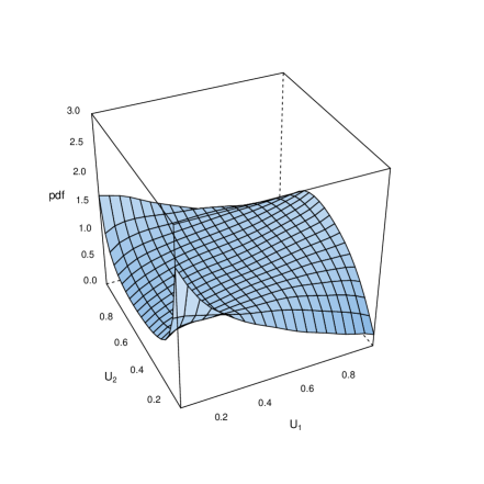
(a) 3D Plot: Density of the Copula

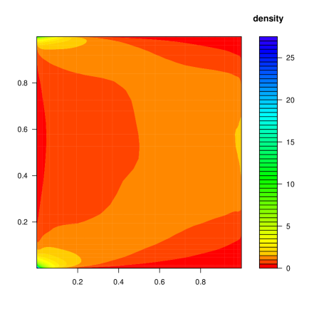
(b) Contour: Density of the Copula

Figure 1: Density estimation of the copula of $(N^{*},M)$ using a kernel density estimation

Let $(U_{1},U_{2})$ be a random vector sampled from $\widehat{C}^{*}$ in Figure 1. As shown from the figure, for the lower $U_{1}$, the density of the copula tends to be smaller at the center of $U_{2}$. On the contrary, for the higher $U_{1}$, the density of the copula tends to be larger at the center of $U_{2}$. Clearly, the density plots in Figure 1 reflect the fact that the conditional variance of $M$ shrinks as $N$ rises, which captures the most eminent feature of the copula of $(N,M)$.

In conclusion, the choice of the copula family to provide a suitable dependence structure between $N$ and $M$ described in Example 1 can be difficult. We consider that no existing parametric copula family can reflect the property described in Example 1 accurately. One may consider using the non-parametric bivariate copula approach as in Chen and Huang, 2007b ; however, this also has difficulties to provide a straightforward interpretation of the dependence, as shown in Example 1, as long as $(N,M)$ is modeled.

In the subsequent sections, rather than directly providing the dependence of the summarized data $(N,M)$, we provide the dependence structure of the micro-level data $(N,Y_{1},\cdots,Y_{N})$ using a copula method. Such an approach requires access to full data, whereas the approach in Example 1 only requires the summarized data.

4 Correlation Matrix for Frequency and Individual Severities

This section presents two useful correlation matrices to describe the dependence of $(N,Y_{1},\cdots,Y_{N})$.

4.1 Equicorrelation matrix

We study a correlation matrix that has a common pairwise correlation for individual severities $(Y_{1},\cdots,Y_{N})$. Based on this, we investigate an extended correlation matrix for $(N,Y_{1},\cdots,Y_{N})$.

Definition 1.

For $\rho_{1},\rho_{2}\in[-1,1]$, define the following matrices.

1. For any positive integer $k$, define a $k\times k$ matrix $\boldsymbol{\Sigma}_{\rho_{2}}^{[k,1]}$

   $$\left[\boldsymbol{\Sigma}_{\rho_{2}}^{[k,1]}\right]_{i,j}:=\begin{cases}1,&\hbox{if}\quad i=j\\ \rho_{2},&\hbox{if}\quad i\neq j\\ \end{cases}$$

   for $i,j=1,\cdots,k$.

2. For any non-negative integer $k$, define a $(k+1)\times(k+1)$ matrix $\boldsymbol{\Sigma}_{\rho_{1},\rho_{2}}^{[k,1]}$

   $$\boldsymbol{\Sigma}_{\rho_{1},\rho_{2}}^{[k,1]}:=\begin{cases}\left(\begin{array}[]{cc}1&\rho_{1}\left({\bf 1}_{k}\right)^{\mathrm{T}}\\ \rho_{1}{\bf 1}_{k}&\boldsymbol{\Sigma}_{\rho_{2}}^{[k,1]}\\ \end{array}\right),&k=1,2,\cdots,;\\ 1,&k=0;\\ \end{cases}$$

   where ${\bf 1}_{k}$ is a column vector of $1$ with length $k$.

In matrix form, $\boldsymbol{\Sigma}_{\rho_{2}}^{[k,1]}$ and $\boldsymbol{\Sigma}_{\rho_{1},\rho_{2}}^{[k,1]}$ in Definition 1 are written as

$$\boldsymbol{\Sigma}_{\rho_{2}}^{[k,1]}=\left(\begin{array}[]{ccccc}1&\rho_{2}&\rho_{2}&\cdots&\rho_{2}\\ \rho_{2}&1&\rho_{2}&\cdots&\rho_{2}\\ \rho_{2}&\rho_{2}&1&\cdots&\rho_{2}\\ \vdots&\vdots&\vdots&\ddots&\vdots\\ \rho_{2}&\rho_{2}&\rho_{2}&\cdots&1\\ \end{array}\right)\quad\hbox{and}\quad\boldsymbol{\Sigma}_{\rho_{1},\rho_{2}}^{[k,1]}=\left(\begin{array}[]{cccccc}1&\rho_{1}&\rho_{1}&\rho_{1}&\cdots&\rho_{1}\\ \rho_{1}&1&\rho_{2}&\rho_{2}&\cdots&\rho_{2}\\ \rho_{1}&\rho_{2}&1&\rho_{2}&\cdots&\rho_{2}\\ \rho_{1}&\rho_{2}&\rho_{2}&1&\cdots&\rho_{2}\\ \vdots&\vdots&\vdots&\vdots&\ddots&\vdots\\ \rho_{1}&\rho_{2}&\rho_{2}&\rho_{2}&\cdots&1\\ \end{array}\right).$$

The following proposition provides the determinants of $\boldsymbol{\Sigma}_{\rho_{2}}^{[k,1]}$ and $\boldsymbol{\Sigma}_{\rho_{1},\rho_{2}}^{[k,1]}$.

Proposition 1.

For any non-negative integer $k$ and $\rho_{1},\rho_{2}\in(-1,1)$, we have

$${\rm det}\left(\boldsymbol{\Sigma}_{\rho_{2}}^{[k,1]}\right)=\left(1+(k-1)\rho_{2}\right)\left(1-\rho_{2}\right)^{k-1}$$ (6)

and

$${\rm det}\left(\boldsymbol{\Sigma}_{\rho_{1},\rho_{2}}^{[k,1]}\right)=\left[1+(k-1)\rho_{2}-k(\rho_{1})^{2}\right](1-\rho_{2})^{k-1}.$$

The proof is given in Appendix A. We also provide the inverse of $\boldsymbol{\Sigma}_{\rho_{2}}^{[k,1]}$ and $\boldsymbol{\Sigma}_{\rho_{1},\rho_{2}}^{[k,1]}$.

Proposition 2.

Let $k$ be any non-negative integer and $\rho_{1},\rho_{2}\in(-1,1)$. If ${\rm det}\left(\boldsymbol{\Sigma}_{\rho_{2}}^{[k,1]}\right)\neq 0$, then the inverse matrix of $\boldsymbol{\Sigma}_{\rho_{2}}^{[k,1]}$ is

$$\left(\boldsymbol{\Sigma}_{\rho_{2}}^{[k,1]}\right)^{-1}=\frac{1}{1-\rho_{2}}\left[\boldsymbol{I}_{k}-\frac{\rho_{2}}{1+(k-1)\rho_{2}}\boldsymbol{J}_{k\times k}\right],$$ (7)

where $\boldsymbol{J}_{k\times k}$ is a $k\times k$ matrix of ones. Furthermore, if ${\rm det}\left(\boldsymbol{\Sigma}_{\rho_{1},\rho_{2}}^{[k,1]}\right)\neq 0$, then

$$\left[\boldsymbol{\Sigma}_{\rho_{1},\rho_{2}}^{[k,1]}\right]^{-1}=\left(\begin{array}[]{cc}\frac{\rho_{1}^{2}k}{1+(k-1)\rho_{2}-k\rho_{1}^{2}}&\frac{\rho_{1}}{1+(k-1)\rho_{2}-k\rho_{1}^{2}}\boldsymbol{1}_{k}^{\mathrm{T}}\\ \frac{\rho_{1}}{1+(k-1)\rho_{2}-k\rho_{1}^{2}}\boldsymbol{1}_{k}&\frac{1}{1-\rho_{2}}\left[\boldsymbol{I}_{k}-\frac{\rho_{2}-\rho_{1}^{2}}{1+(k-1)\rho_{2}-k\rho_{1}^{2}}\boldsymbol{J}_{k\times k}\right]\\ \end{array}\right).$$ (8)

The proof is given in Appendix A. The following theorem provides the condition for $\boldsymbol{\Sigma}_{\rho_{2}}^{[k,1]}$ and $\boldsymbol{\Sigma}_{\rho_{1},\rho_{2}}^{[k,1]}$ to be positive definite.

Theorem 1.

Let $k$ be any positive integer and $\rho_{1},\rho_{2}\in(-1,1)$. Then, $\boldsymbol{\Sigma}_{\rho_{2}}^{[k,1]}$ is positive definite if and only if $\rho_{2}$ satisfies

$$1+\rho_{2}(k-1)>0.$$ (9)

Similarly, $\boldsymbol{\Sigma}_{\rho_{1},\rho_{2}}^{[k,1]}$ is positive definite if and only if $\rho_{1}$ and $\rho_{2}$ satisfy

$$k(\rho_{1})^{2}-1<(k-1)\rho_{2}.$$ (10)

The proof is given in Appendix A. For any positive integer $k$ and $\rho_{1}\in(-1,1)$, define

$$L_{\rho_{1},1}(k)=\begin{cases}\frac{k(\rho_{1})^{2}-1}{k-1},&k>1;\\ -1,&\hbox{otherwise}.\end{cases}$$

In Figure 2, the shaded area of $(\rho_{1},\rho_{2})$ guarantees that $\boldsymbol{\Sigma}_{\rho_{1},\rho_{2}}^{[k,1]}$ is positive definite for different $k$. As shown in the figure, the shaded area shrinks as $k$ increases. The following corollary, which extends Theorem 1, formally describes such an observation.

Corollary 1.

Let $k_{1},\cdots,k_{z}$ be non-negative integers. Then, we have the following results.

1. For $\rho_{1},\rho_{2}\in[-1,1]$, the correlation matrices

   $$\boldsymbol{\Sigma}_{\rho_{1},\rho_{2}}^{[k_{1},1]},\cdots,\boldsymbol{\Sigma}_{\rho_{1},\rho_{2}}^{[k_{z},1]}$$

   are positive definite if and only if $\rho_{1}$ and $\rho_{2}$ satisfy

   $$L_{\rho_{1},1}(\max\{k_{1},\cdots,k_{z}\})<\rho_{2}<1.$$ (11)

2. If $\rho_{1}$ and $\rho_{2}$ satisfy

   $$\rho_{1}^{2}<\rho_{2}<1,$$

   then

   $$\boldsymbol{\Sigma}_{\rho_{1},\rho_{2}}^{[k,1]}$$

   is positive definite for any non-negative integer $k$.

For the proof, the first part comes from the fact that for $\rho_{1}\in(-1,1)$, $L_{\rho_{1},1}(k)$ is a non-decreasing function of $k$ for $k\geq 1$. The second part is the result from

$$\lim\limits_{k\rightarrow\infty}L_{\rho_{1},1}(k)=\rho_{1}^{2}$$

and the first part.

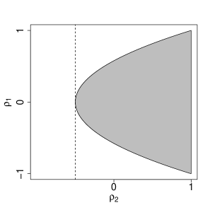
(a) $k=3$

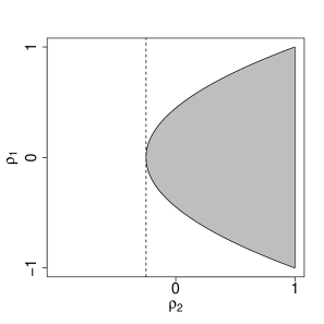
(b) $k=5$

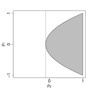
(c) $k=10$

Figure 2: Area of $(\rho_{1},\rho_{2})$ satisfying (10) for different values of the $k$’s

4.2 Autoregressive correlation matrix

We study a correlation matrix that has an autoregressive correlation structure for individual severities $(Y_{1},\cdots,Y_{N})$. Based on this, we investigate an extended correlation matrix for $(N,Y_{1},\cdots,Y_{N})$.

Definition 2.

For $\rho_{1},\rho_{2}\in[-1,1]$, define the following matrices.

1. For any positive integer $k$, define a $k\times k$ matrix $\boldsymbol{\Sigma}_{\rho_{2}}^{[k,2]}$ as

   $$\left[\boldsymbol{\Sigma}_{\rho_{2}}^{[k,2]}\right]_{i,j}:=\begin{cases}1,&\hbox{if}\quad i=j\\ \rho_{2}^{\left|i-j\right|},&\hbox{if}\quad i\neq j\\ \end{cases}$$

   for $i,j=1,\cdots,k$.

2. For any non-negative integer $k$, define a $(k+1)\times(k+1)$ matrix $\boldsymbol{\Sigma}_{\rho_{1},\rho_{2}}^{[k,2]}$ as

   $$\boldsymbol{\Sigma}_{\rho_{1},\rho_{2}}^{[k,2]}:=\begin{cases}\left(\begin{array}[]{cc}1&\rho_{1}\left({\bf 1}_{k}\right)^{\mathrm{T}}\\ \rho_{1}{\bf 1}_{k}&\boldsymbol{\Sigma}_{\rho_{2}}^{[k,2]}\\ \end{array}\right),&k=1,2,\cdots,;\\ 1,&k=0;\\ \end{cases}$$

   where ${\bf 1}_{k}$ is a column vector of $1$ with length $k$.

In matrix form, $\boldsymbol{\Sigma}_{\rho_{2}}^{[k,2]}$ and $\boldsymbol{\Sigma}_{\rho_{1},\rho_{2}}^{[k,2]}$ in Definition 2 are written as

$$\boldsymbol{\Sigma}_{\rho_{2}}^{[k,2]}=\left(\begin{array}[]{ccccc}1&(\rho_{2})^{1}&(\rho_{2})^{2}&\cdots&(\rho_{2})^{k-1}\\ (\rho_{2})^{1}&1&(\rho_{2})^{1}&\cdots&(\rho_{2})^{k-2}\\ (\rho_{2})^{2}&(\rho_{2})^{1}&1&\cdots&(\rho_{2})^{k-3}\\ \vdots&\vdots&\vdots&\ddots&\vdots\\ (\rho_{2})^{k-1}&(\rho_{2})^{k-2}&(\rho_{2})^{k-3}&\cdots&1\\ \end{array}\right)$$

and

$$\boldsymbol{\Sigma}_{\rho_{1},\rho_{2}}^{[k,2]}=\left(\begin{array}[]{cccccc}1&\rho_{1}&\rho_{1}&\rho_{1}&\cdots&\rho_{1}\\ \rho_{1}&1&(\rho_{2})^{1}&(\rho_{2})^{2}&\cdots&(\rho_{2})^{k-1}\\ \rho_{1}&(\rho_{2})^{1}&1&(\rho_{2})^{1}&\cdots&(\rho_{2})^{k-2}\\ \rho_{1}&(\rho_{2})^{2}&(\rho_{2})^{1}&1&\cdots&(\rho_{2})^{k-3}\\ \vdots&\vdots&\vdots&\vdots&\ddots&\vdots\\ \rho_{1}&(\rho_{2})^{k-2}&(\rho_{2})^{k-3}&\cdots&1\\ \end{array}\right).$$

The following proposition provides the determinants of $\boldsymbol{\Sigma}_{\rho_{2}}^{[k,2]}$ and $\boldsymbol{\Sigma}_{\rho_{1},\rho_{2}}^{[k,2]}$.

Proposition 3.

For $\rho_{1},\rho_{2}\in(-1,1)$ and any non-negative integer $k$, we have

$${\rm det}\left(\boldsymbol{\Sigma}_{\rho_{2}}^{[k,2]}\right)=(1-\rho_{2}^{2})^{k}$$

and

$${\rm det}\left(\boldsymbol{\Sigma}_{\rho_{1},\rho_{2}}^{[k,2]}\right)=1-\rho_{1}^{2}\left(k-2\rho_{2}(k-1)+\rho_{2}^{2}(k-2)\right).$$

The proof is given in Appendix A. We also provide the following well-known result without a proof.

Proposition 4.

If ${\rm det}\left(\boldsymbol{\Sigma}_{\rho_{2}}^{[k,2]}\right)\neq 0$, then

$$(1-\rho_{2}^{2})\left[\left(\boldsymbol{\Sigma}_{\rho_{2}}^{[k,2]}\right)^{-1}\right]_{i,j}=\begin{cases}1,&(i,j)=(1,1)\quad\hbox{or}\quad(i,j)=(k,k);\\ 1+\rho_{2}^{2},&(i,j)\neq(1,1),\quad(i,j)\neq(k,k)\quad\hbox{and}\quad i=j;\\ -\rho_{2},&j=i+1\quad\hbox{or}\quad j=i-1;\\ 0,&\hbox{otherwise}.\end{cases}$$

Although the inverse matrix of $\boldsymbol{\Sigma}_{\rho_{1},\rho_{2}}^{[k,2]}$ can be represented analytically using the Schur complement (Zhang,, 2006), we do not pursue it because its representation is unnecessarily complicated. By contrast, the condition for $\boldsymbol{\Sigma}_{\rho_{1},\rho_{2}}^{[k,2]}$ to be positive definite is succinct, as described in the following theorem. The proof is given in Appendix A.

Theorem 2.

Consider $\rho_{1},\rho_{2}\in(-1,1)$. Then, for a positive integer $k$, $\boldsymbol{\Sigma}_{\rho_{2}}^{[k,2]}$ is positive definite for any $\rho_{1},\rho_{2}\in(-1,1)$. Furthermore, for a non-negative integer $k$, $\boldsymbol{\Sigma}_{\rho_{1},\rho_{2}}^{[k,2]}$ is positive definite for any $\rho_{1},\rho_{2}\in(-1,1)$.

5 Conditional Collective Risk Model

This section presents the dependent collective risk model for positive frequency, which is called the “conditional collective risk model” throughout this paper. In Section 6, we provide a generalized collective risk model that allows zero frequency. Consider the positive frequency and severities:

$$N^{+}\quad\hbox{and}\quad\left\{Y_{1},Y_{2},\cdots\right\}.$$ (12)

Suppose that $n$ and $k$ are positive integers in $\mathbb{N}\times\mathbb{N}$. The distribution function for positive frequency and severities is denoted by

$${\mathbb{P}}\left(N^{+}\leq n,\boldsymbol{Y}^{[k]}\leq\boldsymbol{y}^{[k]}\right).$$ (13)

$k$ in (13) can be determined independently of $N^{+}$. Cossette et al., (2018) studies a similar model, (13), with $k=N^{+}$, but we allow $k$ to be any positive integer. For example, we allow studying the distributions of $\left(N^{+},Y^{[1]}\right)=\left(N^{+},Y_{1}\right)$ and $\left(N^{+},Y^{[2]}\right)=\left(N^{+},Y_{1},Y_{2}\right)$ at the same time. From the condition that the former should be obtained from the latter by integrating it with respect to $Y_{2}$, in general, we require the distribution in (13) to satisfy that for any $k_{1}<k_{2}$, ${\mathbb{P}}\left(N^{+}\leq n,\boldsymbol{Y}^{[k_{1}]}\leq\boldsymbol{y}^{[k_{1}]}\right)$ is derived from ${\mathbb{P}}\left(N^{+}\leq n,\boldsymbol{Y}^{[k_{2}]}\leq\boldsymbol{y}^{[k_{2}]}\right)$ by taking the integration.

Conditional Model 1.

Let $N^{+}\sim F_{1}^{+}$ be a non-degenerate positive integer-valued random variable, with the probability mass function $f_{1}$. Then, we define the joint distribution of $(N^{+},\boldsymbol{Y}^{[k]})$ as satisfying

$$(N^{+},\boldsymbol{Y}^{[k]})\sim H_{k}=C_{k+1}(F_{1}^{+},F_{2},\cdots,F_{2}),\\$$ (14)

for any positive integer $k$, where $F_{2}$ is non-negative continuous distribution that has $f_{2}$ as a probability density function. Here, $C_{k+1}$ is a $(k+1)$-dimensional copula satisfying the following inheritance property: for any $k_{1}<k_{2}$,

$$C_{k_{1}+1}\left(u_{1},\cdots,u_{k_{1}+1}\right)=C_{k_{2}+1}\left(u_{1},\cdots,u_{k_{1}+1},1,\cdots,1\right)\quad\hbox{for}\quad u_{1},\cdots,u_{k_{1}+1}\in[0,1].$$ (15)

For the two copulas $C_{k_{1}+1}$ and $C_{k_{2}+1}$ satisfying the inheritance property, the corresponding distributions $H_{k_{1}+1}$ and $H_{k_{2}+1}$ also satisfy the inheritance property. The copula models that we present in the following subsections satisfy such an inheritance property. In contrast to ours, Cossette et al., (2018)’s model does not require condition (15) to be satisfied. In terms of parameter estimation, our model and Cossette et al., (2018)’s model, which have the same marginal distribution functions and copula functions, provide the same likelihood function because we always have $k=n^{+}$ in real observations. However, to interpret and construct the dependence structure, allowing $k$ to be any positive integer as well as having the condition in (15), which is essentially the same as adding an assumption to the unobserved data, is critical, as commented in Remark 1.

The shared random effect model in Hernández-Bastida et al., (2009), Baumgartner et al., (2015), and Oh et al., (2019) and two-step frequency-severity model of Garrido et al., (2016), Park et al., (2018), and Jeong et al., (2019) require the distribution of individual severity to be in the EDF. Since these models require modeling the dependence between frequency and average severity (or aggregate severity), as mentioned by Garrido et al., (2016) and Oh et al., (2019), the EDF assumption on individual severities is required to derive average severity. On the contrary, since our model does not require modeling the dependence between frequency and average severity, it allows $F_{2}$ to be any distribution function, including a heavy-tailed distribution function.

Similar to Cossette et al., (2018), for a positive integer $k$, the joint density function in Conditional Model 1 can be written as

$$\frac{\partial^{k}}{\partial y_{1}\cdots\partial y_{k}}\left(H_{k}\left(n,\boldsymbol{y}^{[k]}\right)-H_{k}\left(n-1,\boldsymbol{y}^{[k]}\right)\right)$$ (16)

$$\quad\quad\quad\quad\quad=\left({\mathbb{P}}\left(N^{+}\leq n\big{|}\boldsymbol{y}^{[k]}\right)-{\mathbb{P}}\left(N^{+}\leq n-1\big{|}\boldsymbol{y}^{[k]}\right)\right)f_{\boldsymbol{Y}^{[k]}}(\boldsymbol{y}^{[k]})$$

for $n\in\mathbb{Z}$ and $\boldsymbol{y}^{[k]}\in\mathbb{R}^{k}$, where $f_{\boldsymbol{Y}^{[k]}}:\mathbb{R}_{+}^{k}\mapsto\mathbb{R}_{+}$ is the probability density function of $\boldsymbol{Y}^{[k]}$. The computational complexity of (16) depends on the choice of the $(k+1)$-dimensional copula $C_{k+1}$. In particular, the conditional distribution of $N^{+}$ in (16) is involved in the integration of the copula, which increases the complexity of the estimation procedure. In the cases of the Gaussian copula and t-copula, the conditional distribution parts in (16) are relatively easy to compute as well as provide an intuitive interpretation of the dependence structure using the form of the covariance matrix. In this section, we present the Gaussian copula and t-copula versions of Conditional Model 1 in detail.

5.1 Gaussian copula model

In the following, we provide the distribution of $(N^{+},\boldsymbol{Y}^{[k]})$ for a positive integer $k$ based on the Gaussian copula family with the equicorrelation matrix, $\boldsymbol{\Sigma}_{\rho_{1},\rho_{2}}^{[k,z]}$ for $z=1$, and with the autoregressive correlation matrix, $\boldsymbol{\Sigma}_{\rho_{1},\rho_{2}}^{[k,z]}$ for $z=2$.

Conditional Model 2.

Let $N^{+}\sim F_{1}^{+}$ be a non-degenerate positive integer-valued random variable, with the probability mass function $f_{1}$. Consider the positive definite matrices

$$\boldsymbol{\Sigma}_{\rho_{2}}^{[k,z]}\quad\hbox{and}\quad\boldsymbol{\Sigma}_{\rho_{1},\rho_{2}}^{[k,z]}$$

for $z=1,2$. We assume

$$(\rho_{1},\rho_{2})\in\left\{(\rho_{1},\rho_{2})\in(-1,1)^{2}\big{|}\rho_{1}^{2}<\rho_{2}<1\right\}$$ (17)

for $z=1$, and assume

$$(\rho_{1},\rho_{2})\in(-1,1)^{2}$$ (18)

for $z=2$. Then, for the given correlation matrix structure $z\in\{1,2\}$, we define the joint distribution of $(N^{+},\boldsymbol{Y}^{[k]})$ as satisfying

$$(N^{+},\boldsymbol{Y}^{[k]})\sim H_{N^{+},\boldsymbol{Y}^{[k]}}=C_{\boldsymbol{\Sigma}_{\rho_{1},\rho_{2}}^{[k,z]}}(F_{1}^{+},F_{2},\cdots,F_{2}),\\$$ (19)

for any positive integer $k$, where $F_{2}$ is a non-negative continuous distribution that has $f_{2}$ as a probability density function. Here, $C_{\boldsymbol{\Sigma}_{\rho_{1},\rho_{2}}^{[k,z]}}$ is a Gaussian copula, with a corresponding density function denoted as $c_{\boldsymbol{\Sigma}_{\rho_{1},\rho_{2}}^{[k,z]}}$ and correlation matrix $\boldsymbol{\Sigma}_{\rho_{1},\rho_{2}}^{[k,z]}$.

It is straightforward to check that the copula

$$C_{\boldsymbol{\Sigma}_{\rho_{1},\rho_{2}}^{[k,z]}},\quad\hbox{for}\quad z=1,2$$

satisfies the condition in (15). The following lemma shows the explicit form of the density function of Conditional Model 2.

Lemma 1.

Considering the frequency and severities in Conditional Model 2, for each $z=1,2$, we have the following results.

1. For a positive integer $k$, the joint density function is given by

   $$h_{N^{+},\boldsymbol{Y}^{[k]}}(n,\boldsymbol{y}^{[k]})$$ (20)

   $$\quad=f_{\boldsymbol{Y}^{[k]}}(\boldsymbol{y}^{[k]})\left(\Phi\left(\frac{\Phi^{-1}(F_{1}^{+}(n))-\mu_{[k,z]}}{\sigma_{[k,z]}}\right)-\Phi\left(\frac{\Phi^{-1}(F_{1}^{+}(n-1))-\mu_{[k,z]}}{\sigma_{[k,z]}}\right)\right)$$

   for $n\in\mathbb{Z}$ and $\boldsymbol{y}^{[k]}\in\mathbb{R}^{k}$, where $f_{\boldsymbol{Y}^{[k]}}$ is a density function given as

   $$f_{\boldsymbol{Y}^{[k]}}(y_{1},\cdots,y_{k})=c_{\boldsymbol{\Sigma}_{\rho_{2}}^{[k,z]}}(F_{2}(y_{1}),\cdots,F_{2}(y_{k}))\prod_{i=1}^{k}f_{2}(y_{i}),$$ (21)

   which is the probability density function of the cumulative distribution function $C_{\boldsymbol{\Sigma}_{\rho_{2}}^{[k,z]}}(F_{2},\cdots,F_{2})$. Here, $\mu_{[k,z]}$ and $\sigma_{[k,z]}$ are defined as

   $$\mu_{[k,z]}:=\left(\rho_{1}\boldsymbol{1}_{k}^{\mathrm{T}}\right)\left(\boldsymbol{\Sigma}_{\rho_{2}}^{[k,z]}\right)^{-1}\left(\Phi^{-1}(F_{2}(y_{1})),\cdots,\Phi^{-1}(F_{2}(y_{k}))\right)^{\mathrm{T}}$$ (22)

   and

   $$\sigma_{[k,z]}:=\sqrt{1-\left(\rho_{1}\boldsymbol{1}_{k}^{\mathrm{T}}\right)\left(\boldsymbol{\Sigma}_{\rho_{2}}^{[k,z]}\right)^{-1}\left(\rho_{1}\boldsymbol{1}_{k}\right)}.$$ (23)

2. For a positive integer $k$, the conditional density function of is given $\boldsymbol{Y}^{[k]}$ for given $N^{+}=n$ is

   $$h_{\boldsymbol{Y}^{[k]}\big{|}N^{+}}\left(\boldsymbol{Y}^{[k]}\big{|}n\right)$$ (24)

   $$\quad\quad\quad=\frac{f_{\boldsymbol{Y}^{[k]}}(\boldsymbol{y}^{[k]})}{f_{1}^{+}(n)}\left(\Phi\left(\frac{\Phi^{-1}(F_{1}^{+}(n))-\mu_{[k,z]}}{\sigma_{[k,z]}}\right)-\Phi\left(\frac{\Phi^{-1}(F_{1}^{+}(n-1))-\mu_{[k,z]}}{\sigma_{[k,z]}}\right)\right).$$

The proof in given in Appendix B. Conditional Model 2 has an advantage when investigating the degree of dependence among the variables via Spearman’s rho. The definition of Spearman’s rho is first given below.

Definition 3.

Define Spearman’s rho of $(V_{1},V_{2})\sim C(G_{1},G_{2})$ for some bivariate copula $C$ and the marginal distributions $G_{1}$ and $G_{2}$ as

$$\rho(V_{1},V_{2})=12\int\int C(G_{1}(v_{1}),G_{2}(v_{2}))-G_{1}(v_{1})G_{2}(v_{2}){\rm d}v_{1}{\rm d}v_{2}.$$

For the details on Spearman’s rho, see Nelsen, (2006). Spearman’s rho in Conditional Model 2 can be obtained from the following results.

Corollary 2.

Consider the frequency and severities defined in Conditional Model 2. Then, for each $z=1,2$, we have the following results.

1. Spearman’s rho between $N^{+}$ and $Y_{j}$ can be calculated as

   $$\rho(N^{+},Y_{j})=\sum\limits_{n=0}^{\infty}\int_{0}^{\infty}12\left[C_{\rho_{1}}(F_{1}^{+}(n),F_{2}(y))-F_{1}^{+}(n)F_{2}(y)\right]f_{1}(n)f_{2}(y){\rm d}y$$

   , where $C_{\rho_{1}}$ is the Gaussian copula with the correlation coefficient $\rho_{1}$.

2. Spearman’s rho between $Y_{j_{1}}$ and $Y_{j_{2}}$ can be calculated as

   $$\rho(Y_{j_{1}},Y_{j_{2}})=\frac{6}{\pi}\arcsin\left(\frac{\rho_{2}}{2}\right),\quad\hbox{for}\quad z=1$$

   and

   $$\rho(Y_{j_{1}},Y_{j_{2}})=\frac{6}{\pi}\arcsin\left(\frac{\rho_{2}^{\left|k_{1}-k_{2}\right|}}{2}\right),\quad\hbox{for}\quad z=2$$

   for the positive integers $j_{1}$ and $j_{2}$ satisfying $j_{1}\neq j_{2}$.

The proof of the first part is immediate from the definition, and the proof of the second part can be found in Kruskal, (1958).

Remark 1.

In Conditional Model 1, allowing $k$ to be any integer value makes the definition of the dependence measures such as

$$\rho\left(N^{+},Y_{j}\right)\quad\hbox{and}\quad\rho\left(Y_{j_{1}},Y_{j_{2}}\right),\quad j_{1}\neq j_{2}$$ (25)

in Corollary 2 well defined and interpreted straightforwardly. On the contrary, fixing $k=N^{+}$ as in Cossette et al., (2018) may complicate the interpretation. Indeed, under the model with fixed $k=N^{+}$ only, the definition of the (marginal) dependence measures in (25) may be loose because $Y_{j}$ is defined only when $N^{+}\geq j$. Therefore, the model with fixed $k=N^{+}$ only is suitable to discuss the following conditional versions of the dependence measures

$$\rho\left(N^{+},Y_{j}\big{|}N^{+}\geq j\right)\quad\hbox{and}\quad\rho\left(Y_{j_{1}},Y_{j_{2}}\big{|}N^{+}\geq\max\left\{j_{1},j_{2}\right\}\right),\quad j_{1}\neq j_{2}.$$ (26)

However, interpreting the dependence structure with such dependence measures (26) can be difficult. As a consequence, the interpretation of the (marginal) correlation matrix

$$\boldsymbol{\Sigma}_{\rho_{1},\rho_{2}}^{[k,z]},\quad z=1,2$$

introduced in Section 4 may be difficult under Conditional Model 1 with fixed $k=N^{+}$ only.

5.2 T-copula model

The Gaussian copula is not an inevitable choice for modeling frequency and severities. However, for the convenience of the statistical modeling and estimation, we focus on the copula family specified by the covariance (correlation) matrix only. The elliptical copula family has such a property. Among them, we focus on the t-copula that has gained broad popularity in recent studies.

We first define the $k$-dimensional multivariate t-distribution $\boldsymbol{Z}\sim{\rm MVT}(\boldsymbol{0}_{k},\boldsymbol{\Sigma},{\rm df})$, with scale matrix $\boldsymbol{\Sigma}$, and degrees of freedom $\rm df$, which has the following probability density function:

$$f({\boldsymbol{z}})=\frac{\Gamma\left(\frac{k+{\rm df}}{2}\right)}{\Gamma\left(\frac{\rm df}{2}\right)(\pi{\rm df})^{k/2}\left|\boldsymbol{\Sigma}\right|^{1/2}}\left(1+\frac{1}{\rm df}\boldsymbol{k}^{\mathrm{T}}\boldsymbol{\Sigma}^{-1}\boldsymbol{k}\right)$$

for $\boldsymbol{z}=(z_{1},\cdots,z_{k})\in\mathbb{R}^{k}$. We denote the corresponding t-copula as $C_{{\rm df},\boldsymbol{\Sigma}_{\rho_{1},\rho_{2}}^{[k,1]}}$. We also represent $\Phi_{\rm df}$ and $\phi_{\rm df}$ by the cumulative density function and probability density function of the univariate Student’s t-distribution, respectively. The t-copula version of Conditional Model 1 is provided below.

Conditional Model 3.

Let $N^{+}\sim F_{1}^{+}$ be a positive integer-valued random variable, with the probability mass function $f_{1}^{+}$, and assume (19) and (18) for $z=1$ and $z=2$, respectively. Then, for each $z=1,2$, define the joint distribution of $(N,\boldsymbol{Y}^{[k]})$ as in

$$(N^{+},\boldsymbol{Y}^{[k]})\sim C_{{\rm df},\boldsymbol{\Sigma}_{\rho_{1},\rho_{2}}^{[k,z]}}(F_{1}^{+},F_{2},\cdots,F_{2}),\\$$

for any positive integer $k$, where $F_{2}$ is a non-negative continuous distribution that has $f_{2}$ as a probability density function. Here, $C_{{\rm df},\boldsymbol{\Sigma}_{\rho_{1},\rho_{2}}^{[k,z]}}$ is a t-copula, which has the corresponding density function denoted as $c_{{\rm df},\boldsymbol{\Sigma}_{\rho_{1},\rho_{2}}^{[k,z]}}$, with scale matrix $\boldsymbol{\Sigma}_{\rho_{1},\rho_{2}}^{[k,z]}$ and degree of freedom $\rm df$.

The following result is the t-copula version of Lemma 1.

Lemma 2.

Considering the frequency and severities in Conditional Model 3 with $z=1$ and $z=2$, we have the following results.

1. For a positive integer $k$, the joint density function is given by

   $$h_{N^{+},\boldsymbol{Y}^{[k]}}(n,\boldsymbol{y}^{[k]})$$ (27)

   $$\quad=f_{\boldsymbol{Y}^{[k]}}^{*}(\boldsymbol{y}^{[k]})\left(\Phi_{{\rm df}+k}\left(\frac{\Phi_{\rm df}^{-1}(F_{1}^{+}(n))-\mu_{[k,z]}^{*}}{\sigma_{[k,z]}^{*}}\right)-\Phi_{{\rm df}+k}\left(\frac{\Phi_{\rm df}^{-1}(F_{1}^{+}(n-1))-\mu_{[k,z]}^{*}}{\sigma_{[k,z]}^{*}}\right)\right)$$

   for $n\in\mathbb{N}^{+}$ and $\boldsymbol{y}^{[k]}\in\mathbb{R}^{k}$, where $f_{\boldsymbol{Y}^{[k]}}^{*}(\boldsymbol{y}^{[k]})$ is a density function given as

   $$f_{\boldsymbol{Y}^{[k]}}^{*}(y_{1},\cdots,y_{k})=c_{{\rm df},\boldsymbol{\Sigma}_{\rho_{2}}^{[k,z]}}(F_{2}(y_{1}),\cdots,F_{2}(y_{k}))\prod_{i=1}^{k}f_{2}(y_{i}),$$

   which is the probability density function of the cumulative distribution function $C_{{\rm df},\boldsymbol{\Sigma}_{\rho_{2}}^{[k,z]}}(F_{2},\cdots,F_{2})$. Here, $\mu_{[k,z]}^{*}$ and $\sigma_{[k,z]}^{*}$ are defined as

   $$\mu_{[k,z]}^{*}:=\left(\rho_{1}\boldsymbol{1}_{k}^{\mathrm{T}}\right)\left(\boldsymbol{\Sigma}_{\rho_{2}}^{[k,z]}\right)^{-1}\left(\Phi_{\rm df}^{-1}(F_{2}(y_{1})),\cdots,\Phi_{\rm df}^{-1}(F_{2}(y_{k}))\right)^{\mathrm{T}}$$ (28)

   and

   $$\sigma_{[k,z]}^{*}:=\sigma_{[k,z]}$$ (29)

   $$\quad\times\sqrt{\frac{{\rm df}+\left(\Phi_{\rm df}^{-1}(F_{2}(y_{1})),\cdots,\Phi_{\rm df}^{-1}(F_{2}(y_{k}))\right)\left(\boldsymbol{\Sigma}_{\rho_{2}}^{[k,z]}\right)^{-1}\left(\Phi_{\rm df}^{-1}(F_{2}(y_{1})),\cdots,\Phi_{\rm df}^{-1}(F_{2}(y_{k}))\right)^{\mathrm{T}}}{{\rm df}+k}}.$$

2. For a positive integer $k$, the conditional density function of is given $\boldsymbol{Y}^{[k]}$ for given $N^{+}=n$ is

   $$h_{\boldsymbol{Y}^{[k]}\big{|}N^{+}}\left(\boldsymbol{Y}^{[k]}\big{|}n\right)$$ (30)

   $$\quad\quad\quad=\frac{f_{\boldsymbol{Y}^{[k]}}^{*}(\boldsymbol{y}^{[k]})}{f_{1}^{+}(n)}\left(\Phi_{{\rm df}+k}\left(\frac{\Phi_{\rm df}^{-1}(F_{1}^{+}(n))-\mu_{[k,z]}^{*}}{\sigma_{[k,z]}^{*}}\right)-\Phi_{{\rm df}+k}\left(\frac{\Phi_{\rm df}^{-1}(F_{1}^{+}(n-1))-\mu_{[k,z]}^{*}}{\sigma_{[k,z]}^{*}}\right)\right).$$

For brevisity, we omit the proof because it is similar to that of Lemma 1.

6 Collective Risk Model with the Observed Data

Conditional Models 2 and 3 cannot be directly applied to real data including zero frequency because they assume that the frequency is positive. In the following, we explain how to modify Conditional Models 2 and 3 to accommodate zero frequency.

Model 1 (Dependent collective risk model).

For each correlation matrix $z=1,2$, consider the frequency and severities defined in Conditional Model 2 or 3. We assume that $R$ is a Bernoulli random variable with success probability $p$, and it is mutually independent of $(N^{+},Y_{1},\cdots,Y_{k})$ for any $k>0$. Define

$$N:=\begin{cases}N^{+},&R=1;\\ 0,&R=0;\\ \end{cases}$$

and its cumulative distribution function and density function as $F_{1}$ and $f_{1}$, respectively. Then, define

$$(N,\boldsymbol{Y}^{[N]}):=\begin{cases}(N,Y_{1},\cdots,Y_{N}),&N\geq 1;\\ 0,&N=0;\\ \end{cases}$$

as a dependent collective risk model.

Model 1 is called the “dependent collective risk model” throughout the paper. The following theorems, which are the corollaries of Lemmas 1 and 2, show the joint density function of $(N,\boldsymbol{Y}^{[N]})$ in Model 1.

Theorem 3.

Consider Model 1 along with Conditional Model 2. Then, for each $z=1,2$, the joint density function of the discrete margin $N$ and continuous margins $\boldsymbol{Y}_{N}$ is given by

$$h(n,\boldsymbol{y}^{[n]})$$ (31)

$$\quad=\begin{cases}p\,f_{\boldsymbol{Y}^{[n]}}(\boldsymbol{y}^{[n]})\left(\Phi\left(\frac{\Phi^{-1}(F_{1}^{+}(n))-\mu_{[n,z]}}{\sigma_{[n,z]}}\right)-\Phi\left(\frac{\Phi^{-1}(F_{1}^{+}(n-1))-\mu_{[n,z]}}{\sigma_{[n,z]}}\right)\right),&n\in\mathbb{N},\quad\boldsymbol{y}^{[n]}\in\mathbb{R}^{n}\\ 1-p,&n=0,\\ \end{cases}$$

where $\mu_{[n,z]}$ and $\sigma_{[n,z]}$ are defined in (22) and (23).

The proof is provided here. (31) is trivial for $n=0$. Now, consider the case for $n>0$. For an observation $(n,y_{1},\cdots,y_{n})$, the corresponding likelihood function is

$$h(n,\boldsymbol{y}^{[n]}) =p\,f_{1}^{+}(n)h_{\boldsymbol{Y}^{[n]}\big{|}N^{+}}(y_{1},\cdots,y_{n}\big{|}n)$$

$$=p\,h_{N^{+},\boldsymbol{Y}^{[n]}}(n,\boldsymbol{y}^{[n]}),$$

where the second equality is from part ii of Lemma 1.

Theorem 4.

Consider Model 1 along with Conditional Model 3. Then, for each $z=1,2$, the joint density function of the discrete margin $N$ and continuous margins $\boldsymbol{Y}_{N}$ is given by

$$h(n,\boldsymbol{y}^{[n]})$$ (32)

$$\quad=\begin{cases}p\,f_{\boldsymbol{Y}^{[n]}}(\boldsymbol{y}^{[n]})\left(\Phi_{{\rm df}+n}\left(\frac{\Phi_{\rm df}^{-1}(F_{1}^{+}(n))-\mu_{[n,z]}^{*}}{\sigma_{[n,z]}^{*}}\right)-\Phi_{{\rm df}+n}\left(\frac{\Phi_{\rm df}^{-1}(F_{1}^{+}(n-1))-\mu_{[n,z]}^{*}}{\sigma_{[n,z]}^{*}}\right)\right),&n\in\mathbb{N},\quad\boldsymbol{y}^{[n]}\in\mathbb{R}^{n}\\ 1-p,&n=0,\\ \end{cases}$$

where $\mu_{[n,z]}^{*}$ and $\sigma_{[n,z]}^{*}$ are defined in (28) and (29).

For brevity, we omit the proof because it is the same as in Theorem 3.

6.1 Derivation of some useful quantities

Using Lemma 5 in the Appendix B, the following proposition shows how to derive some useful quantities from Model 1.

Proposition 5.

Consider Model 1 along with either Conditional Model 2 or Conditional Model 3. Then, we have

$${\mathbb{E}}\left[S\right]={\mathbb{E}}\left[\sum_{j=1}^{N}Y_{j}\right]=p\sum\limits_{n=1}^{\infty}n\int_{0}^{\infty}y\,h_{N^{+},\boldsymbol{Y}^{[1]}}(n,y){\rm d}y$$

and

$${\rm cov}\left[N,S\right]=p\sum\limits_{n=1}^{\infty}n^{2}\int_{0}^{\infty}yh_{N^{+},\boldsymbol{Y}^{[1]}}(n,y){\rm d}y-\left(p\sum\limits_{n=1}^{\infty}nf_{N^{+}}(n)\right)\left(p\sum\limits_{n=1}^{\infty}n\int_{0}^{\infty}y\,h_{N^{+},\boldsymbol{Y}^{[1]}}(n,y){\rm d}y\right),$$

where $h_{N^{+},\boldsymbol{Y}^{[1]}}$ is defined in (20) or (27), depending on the assumptions of Conditional Model 2 or Conditional Model 3 as well as the type of covariance matrix. Furthermore, we have

$${\rm cov}\left[N,M\big{|}N>0\right] =\sum\limits_{n=1}^{\infty}n\int_{0}^{\infty}yh_{N^{+},\boldsymbol{Y}^{[1]}}(n,y){\rm d}y-\left(\sum\limits_{n=1}^{\infty}nf_{N^{+}}(n)\right)\left(\sum\limits_{n=1}^{\infty}n\int_{0}^{\infty}yh_{N^{+},\boldsymbol{Y}^{[1]}}(n,y){\rm d}y\right).$$

The detailed derivation steps of Proposition 5 are given in Appendix C.

6.2 Extension to regression models

We provide regression models for the dependent collective risk model below.

Model 2.

For each individual $i=1,\cdots,I$, consider the dependent collective risk model for

$$(N_{i},\boldsymbol{Y}_{i}^{[N_{i}]}):=\begin{cases}(N_{i},Y_{i1},\cdots,Y_{iN_{i}}),&N_{i}\geq 1;\\ 0,&N_{i}=0;\\ \end{cases}$$

in Model 1. Let $\left(\boldsymbol{x}_{i},\boldsymbol{x}_{i}^{*},\boldsymbol{w}_{i}\right)$ be the given characteristics of the $i$-th policyholder. Consider the following model.

1. For the frequency part, use the hurdle regression model with $N_{it}$. Specifically, use $\boldsymbol{x}_{i}$ and $\boldsymbol{x}_{i}^{*}$ as the explanatory variables for the zero and positive frequency parts, respectively. Denote $\boldsymbol{\beta}$ and $\boldsymbol{\beta}^{*}$ as the corresponding sets of regression coefficients. Specifically,

   $$N_{i}^{+}\sim{F}_{1}^{+}\left(\cdot;\lambda_{i},\psi_{1}\right),\quad\hbox{with}\quad\eta_{1}(\lambda_{i})=\boldsymbol{x}_{i}\boldsymbol{\beta}$$

   and

   $$R_{i}\sim{\rm Ber}\left(p_{i}\right),\quad\hbox{with}\quad\eta_{1}^{*}(p_{i})=\boldsymbol{x}_{i}^{*}\boldsymbol{\beta}^{*}$$

   for some link functions $\eta_{1}$ and $\eta_{1}^{*}$.

2. For the severity part, use the regression model with $Y_{it}$ and $\boldsymbol{w}_{i}$ as the dependent variable and the set of explanatory variables, respectively. Denote $\boldsymbol{\gamma}$ as the corresponding sets of regression coefficients. Specifically, for $N_{i}>0$,

   $$Y_{it}\sim{F}_{2}\left(\cdot\,;\,\xi_{i},\psi_{2}\right),\quad\hbox{with}\quad\eta_{2}(\xi_{i})=\boldsymbol{w}_{i}\boldsymbol{\gamma}$$

   for $t\in\mathcal{N}$ with some link function $\eta_{2}$.

Model 2 is a flexible regression model for frequency and severities. Its marginal distribution of frequency is given as

$$F_{1}(n;\lambda_{i},\psi_{1})=1-p_{i}+p_{i}F_{1}^{+}(n;\lambda_{i},\psi_{1})$$

for $n=0,1,\ldots$. A special case of Model 2 is particularly interesting because it is convenient for statistical estimation. Consider any distribution function $F_{1}$ that can explain the frequency part including zero. Define

$$p_{i}=1-{F}_{1}\left(0;\lambda_{i},\psi_{1}\right)$$

and

$$F_{1}^{+}(n;\lambda_{i},\psi_{1})=\frac{{F}_{1}\left(n;\lambda_{i},\psi_{1}\right)-{F}_{1}\left(0;\lambda_{i},\psi_{1}\right)}{1-{F}_{1}\left(0;\lambda_{i},\psi_{1}\right)}$$

for $n\in\mathbb{N}_{+}$. Then, we have

$$N_{i}\sim F_{1}(\cdot;\lambda_{i},\psi_{1}).$$

We use this model for the simulation and data analysis in the following sections. Specifically, we use the Poisson distribution with mean $\lambda_{i}=\exp(\boldsymbol{x}_{i}\boldsymbol{\beta})$ for $N_{i}$, and Gamma distribution $\xi_{i}=\exp(\boldsymbol{w}_{i}\boldsymbol{\gamma})$ for $Y_{it}$.

7 Numerical Study

We conduct a simulation study to investigate the finite sample properties of the parameter estimates and effect of the dependence between frequency and severity on them for the proposed model. The portfolio of policyholders of size $I=5000$ are generated from the proposed model under 12 scenarios motivated by the real data analysis in Section 8. Table 1 provides the details of the parameter settings. In each simulation, two predictors $\boldsymbol{x}_{i}$ and $\boldsymbol{w}_{i}$ are used and generated from Bernoulli(0.5) independently.

Table 1: Parameter settings for the 12 scenarios

	Parameter
Scenario	$\beta_{0}$	$\beta_{1}$	$\beta_{2}$	$\gamma_{0}$	$\gamma_{1}$	$\gamma_{2}$	$\nu$	$\rho_{1}$	$\rho_{2}$
1	-2.5	0.5	1.0	8	-0.1	0.3	0.7	-0.05	0.10
2	-2.5	0.5	1.0	8	-0.1	0.3	0.7	-0.05	0.05
3	-2.5	0.5	1.0	8	-0.1	0.3	0.7	0.05	0.10
4	-2.5	0.5	1.0	8	-0.1	0.3	0.7	0.05	0.05
5	-2.5	0.5	1.0	8	-0.1	0.3	0.7	0.10	0.10
6	-2.5	0.5	1.0	8	-0.1	0.3	0.7	0.10	0.05
7	-2.5	0.5	1.5	8	-0.1	0.3	0.7	-0.05	0.10
8	-2.5	0.5	1.5	8	-0.1	0.3	0.7	-0.05	0.05
9	-2.5	0.5	1.5	8	-0.1	0.3	0.7	0.05	0.10
10	-2.5	0.5	1.5	8	-0.1	0.3	0.7	0.05	0.05
11	-2.5	0.5	1.5	8	-0.1	0.3	0.7	0.10	0.10
12	-2.5	0.5	1.5	8	-0.1	0.3	0.7	0.10	0.05

For each scenario, Table 2 and Table 3 summarize the simulation results from 500 independent Monte Carlo samples, including the relative bias and mean squared error (MSE) of the parameter estimates. Table 2 indicates that in all the scenarios, the estimates are close to the true parameters of the proposed model and shows that the relative bias and MSE are small. A relative bias larger than 10$\%$ is only observed for $\rho_{2}$ in scenario 5, which has relatively high correlations for $\rho_{1}$ and $\rho_{2}$.

Table 2: Relative bias in $\%$ for all the parameters from the 12 scenarios

	Relative Bias ($\%$)
Scenario	$\beta_{0}$	$\beta_{1}$	$\beta_{2}$	$\gamma_{0}$	$\gamma_{1}$	$\gamma_{2}$	$\nu$	$\rho_{1}$	$\rho_{2}$
1	0.06	0.34	0.01	0.01	-1.57	-0.10	0.19	5.79	8.61
2	0.10	0.35	0.11	0.11	-0.55	-0.59	0.16	0.36	0.42
3	-0.12	-0.57	-0.17	-0.17	-0.60	-0.73	0.23	1.74	6.77
4	0.01	-0.36	0.11	0.11	-4.00	0.46	0.43	0.94	-2.63
5	0.00	0.32	-0.05	-0.05	0.89	-0.77	0.11	1.58	14.90
6	0.02	-0.13	-0.07	-0.07	-1.62	-1.50	0.31	-1.45	-0.83
7	0.01	-0.07	-0.03	-0.03	2.98	1.15	0.12	0.66	-0.08
8	0.03	0.10	-0.08	-0.08	-2.36	0.05	0.11	-1.92	-2.80
9	0.03	0.43	0.04	0.04	0.68	1.50	0.26	1.14	4.61
10	0.16	0.07	0.22	0.22	-1.39	-0.72	0.04	0.98	-0.73
11	-0.10	-0.30	-0.15	-0.15	-0.95	0.40	0.08	1.89	3.16
12	-0.04	-0.03	-0.18	-0.18	-0.80	0.88	0.28	0.68	-2.55

Table 3: Mean absolute error for all the parameters from the 12 scenarios

	MSE
Scenario	$\beta_{0}$	$\beta_{1}$	$\beta_{2}$	$\gamma_{0}$	$\gamma_{1}$	$\gamma_{2}$	$\nu$	$\rho_{1}$	$\rho_{2}$
1	0.0028	0.0020	0.0023	0.0039	0.0033	0.0037	0.0004	0.0008	0.0023
2	0.0028	0.0023	0.0026	0.0041	0.0034	0.0035	0.0003	0.0008	0.0038
3	0.0025	0.0023	0.0024	0.0037	0.0032	0.0035	0.0004	0.0007	0.0027
4	0.0025	0.0022	0.0023	0.0035	0.0030	0.0037	0.0004	0.0008	0.0035
5	0.0022	0.0020	0.0024	0.0038	0.0030	0.0039	0.0003	0.0008	0.0024
6	0.0028	0.0022	0.0025	0.0035	0.0029	0.0037	0.0004	0.0009	0.0034
7	0.0022	0.0016	0.0022	0.0033	0.0022	0.0031	0.0003	0.0005	0.0014
8	0.0025	0.0014	0.0022	0.0031	0.0018	0.0032	0.0002	0.0005	0.0015
9	0.0022	0.0015	0.0022	0.0029	0.0020	0.0032	0.0003	0.0005	0.0013
10	0.0023	0.0013	0.0021	0.0034	0.0023	0.0029	0.0003	0.0006	0.0016
11	0.0023	0.0015	0.0023	0.0038	0.0021	0.0033	0.0002	0.0004	0.0013
12	0.0025	0.0014	0.0022	0.0036	0.0021	0.0030	0.0003	0.0004	0.0016

8 Real Data Analysis

To see the usefulness of the proposed model for examining the dependence structure between (a) frequency and severity and (b) severities, we analyze a real automobile insurance dataset.

8.1 Data

We use the automobile insurance data provided by the Massachusetts Executive Office of Energy and Environmental Affairs, which were used by Ferreira Jr and Minikel, (2012). The data contain the history of automobile insurance claims in 2006 in the state of Massachusetts. With $15$ variables, the data consist of information on $3,991,012$ insured persons. The dataset also shows the $681,423$ claims of liability and personal injury protection coverage claim information with $10$ variables. Each policyholder has information on the number of claims, individual claim amounts with the date of accidents, and covariates. Among the observations, we randomly sample $1,500,000$ policyholders whose accidents occurred before 2008 and who have automobile insurance providing third party liability coverage for property damage and bodily injury. The first $1,000,000$ observations are used as the training data to develop the model and the rest is reserved as the hold-out sample for validation purposes. We use the following two covariates, CLASS and TERRITORY, for the risk classification. CLASS denotes five groups divided by policyholder characteristics (A: adults, B: business, I: $<3$ years of experience, M: $3\sim 6$ years of experience, S: senior citizens). TERRITORY denotes six territory groups divided by the driving characteristics (1: least risky to 6: most risky territory). Table 4 shows the mean frequency and mean severity per claim of the data categorized by CLASS and TERRITORY. Full details of the covariates used can be found in the online supplement and in Ferreira Jr and Minikel, (2012).

Table 4: Table of mean frequency and mean severity per claim (percentage of observations in brackets)

		CLASS
		A	B	I	M	S
	1	0.046 / 3241	0.046 / 1513	0.078 / 4186	0.058 / 4547	0.048 / 3426
		(13.69%)	(0.31%)	(1.17%)	(0.87%)	(2.89%)
	2	0.046 / 3833	0.046 / 5516	0.070 / 3091	0.066 / 3501	0.049 / 3006
		(13.82%)	(0.30%)	(1.13%)	(0.94%)	(3.16%)
TERRITORY	3	0.048 / 3933	0.033 / 2180	0.085 / 4724	0.055 / 3977	0.048 / 4196
		(8.19%)	(0.15%)	(0.58%)	(0.55%)	(1.67%)
	4	0.051 / 3702	0.060 / 4431	0.097 / 3809	0.061 / 3601	0.060 / 4153
		(14.88%)	(0.27%)	(1.00%)	(0.96%)	(3.01%)
	5	0.055 / 4042	0.083 / 2949	0.093 / 4052	0.084 / 4538	0.061 / 3812
		(14.11%)	(0.21%)	(0.84%)	(0.94%)	(2.72%)
	6	0.062 / 4249	0.111 / 2979	0.107 / 4264	0.092 / 4968	0.070 / 4412
		(8.87%)	(0.11%)	(0.60%)	(0.71%)	(1.35%)

8.2 Estimation results

We apply Model 2 to the Massachusetts automobile data, where $N_{i}$ and $Y_{it}$ follow a Poisson distribution and a gamma distribution, respectively. Table 5 summarizes the estimation results for the model. Based on the results, the class and territory groups are important factors for both the frequency and the severity parts. The regression coefficients for the territory group show increasing patterns from the least risky to the most risky area in both the frequency and the severity parts. The class group with less experience of driving (class=I) shows more accidents and the claim amount in that group tends to be higher than that in the other groups. In the dependent collective risk model, the dependence between frequency and severity is measured by the parameter $\rho_{1}$. Its estimate is $-0.018$ with a 95$\%$ confidence interval of $(-0.031,-0.005)$, suggesting a significant negative correlation between the number of accidents and claim size. Furthermore, this dependence seems weaker than the dependence between severities $\rho_{2}$.

Table 5: Estimation results

Parameter	Est	Std. error	95$\%$ CI
Frequency part
Intercept	-3.295	0.012	-3.319	-3.270
territory=2	0.084	0.016	0.052	0.116
territory=3	0.121	0.018	0.085	0.157
territory=4	0.213	0.016	0.182	0.243
territory=5	0.326	0.015	0.296	0.356
territory=6	0.455	0.016	0.423	0.487
class=B	0.306	0.036	0.235	0.377
class=I	1.029	0.016	0.999	1.060
class=M	0.497	0.018	0.462	0.533
class=S	-0.017	0.013	-0.043	0.008
Severity part
Intercept	8.067	0.014	8.039	8.095
territory=2	0.081	0.019	0.043	0.118
territory=3	0.062	0.022	0.020	0.104
territory=4	0.144	0.018	0.108	0.179
territory=5	0.154	0.018	0.120	0.189
territory=6	0.296	0.019	0.259	0.333
class=B	0.087	0.042	0.005	0.170
class=I	0.115	0.018	0.080	0.151
class=M	0.133	0.021	0.092	0.175
class=S	-0.105	0.015	-0.135	-0.075
$\nu$	0.738	0.004	0.730	0.746
Copula part
$\rho_{1}$	-0.018	0.006	-0.031	-0.005
$\rho_{2}$	0.027	0.001	0.026	0.029

To examine how well the proposed model and Tweedie’s compound Poisson model fit the training dataset, we consider two quantities: expected aggregate severity, ${\mathbb{E}}\left[S\right]$, and the value at risk of aggregate severity at the confidence level $\alpha=0.995$, $VaR_{0.995}(S)$, by risk group defined by the CLASS and TERRITORY variables. Figure 3 and Table 6 report the results. For comparison purposes, we also report the empirical values of ${\mathbb{E}}\left[S\right]$ and $VaR_{0.995}(S)$ (i.e., model-free estimates) for each risk group. It is expected that good models produce ${\mathbb{E}}\left[S\right]$ and $VaR_{0.995}(S)$ close to the corresponding empirical values. Figure 3 shows that both models provide similar estimates of ${\mathbb{E}}\left[S\right]$ and they are close to the empirical values. Although the MSEs of the two estimates of ${\mathbb{E}}\left[S\right]$, at the bottom of Table 6, do not show large differences, the estimates of $VaR_{0.995}(S)$ of both models show substantial differences in MSEs. Specifically, regarding $VaR_{0.995}(S)$, the risk group with class I shows high values within each territory group and it tends to be increasing as the territory becomes riskier. This pattern is also found in Tweedie’s model; however, it overestimates them for most of the risk groups, which makes its MSE larger than that of our proposed model.

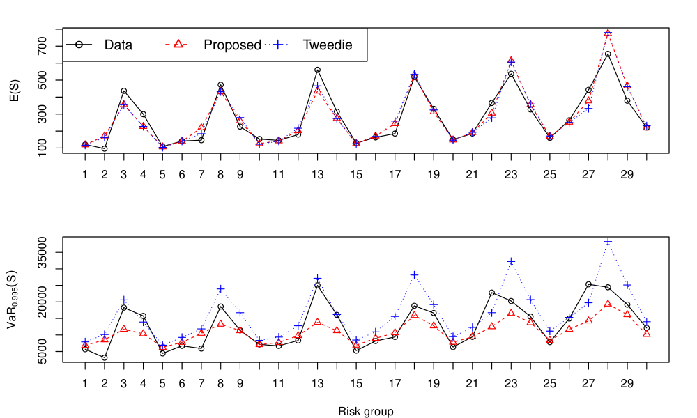
Figure 3: Comparison of ${\mathbb{E}}\left[S\right]$ and $VaR_{0.995}(S)$ by risk group for the training dataset from the Massachusetts automobile data: Empirical value, Proposed model, and Tweedie model

Table 6: Comparison of ${\mathbb{E}}\left[S\right]$ and $VaR_{0.995}(S)$ by risk group for the training dataset from the Massachusetts automobile data: Empirical value, Proposed model, and Tweedie model

Risk	$TERRITORY$	$CLASS$	Data			Proposed			Tweedie
Group			$E[S]$	$VaR_{\alpha}(S)$		$E[S]$	$VaR_{\alpha}(S)$		$E[S]$	$VaR_{\alpha}(S)$
1	1	A	121	5693		119	6845		117	7903
2	1	B	96	3137		171	8542		162	10133
3	1	I	437	18275		356	11718		356	20618
4	1	M	299	15756		227	10357		227	13917
5	1	S	109	4425		107	6263		104	6900
6	2	A	142	6706		139	7760		141	9262
7	2	B	146	5904		219	10508		184	11842
8	2	I	473	18603		432	13255		432	23934
9	2	M	226	11415		260	11286		279	16734
10	2	S	153	7136		126	7071		122	8361
11	3	A	145	6692		142	7738		141	9357
12	3	B	179	8332		202	9800		217	12778
13	3	I	561	25000		436	13807		466	27135
14	3	M	315	16081		275	11290		273	16172
15	3	S	129	5270		127	6928		126	8456
16	4	A	163	8178		171	8969		168	10928
17	4	B	185	9404		244	10663		259	15605
18	4	I	519	18828		529	15908		534	28154
19	4	M	331	16643		313	12778		324	19202
20	4	S	150	6339		148	7797		146	9498
21	5	A	186	9429		191	9439		193	12277
22	5	B	366	22817		305	12494		278	16734
23	5	I	537	20277		615	16528		606	32221
24	5	M	327	15567		356	13709		359	20675
25	5	S	159	7846		168	8381		171	11167
26	6	A	263	14963		252	11698		250	15310
27	6	B	443	25328		378	14252		333	19741
28	6	I	655	24436		775	19352		780	38271
29	6	M	379	19188		466	16152		461	25125
30	6	S	221	12124		218	10163		231	13991
MSE			-			469	4192541		476	9759489

8.3 Validation results

For validation purposes, we compare the two models in terms of the total loss prediction for the 500,000 policyholders in the hold-out sample. Figure 4 presents the predictive distributions of the various models, which are based on 5,000 Monte Carlo simulations under the estimation result from each model. In the figure, the dotted vertical line indicates the actual amount of losses and dashed vertical line indicates the mean estimated total loss. The predictive distribution from our proposed collective risk model has less variation, and its mean is closer to the actual total loss of the hold-out sample. This result can be explained by the fact that there is a significant negative correlation between frequency and individual severity, which is reflected appropriately in our model that allows such dependence.

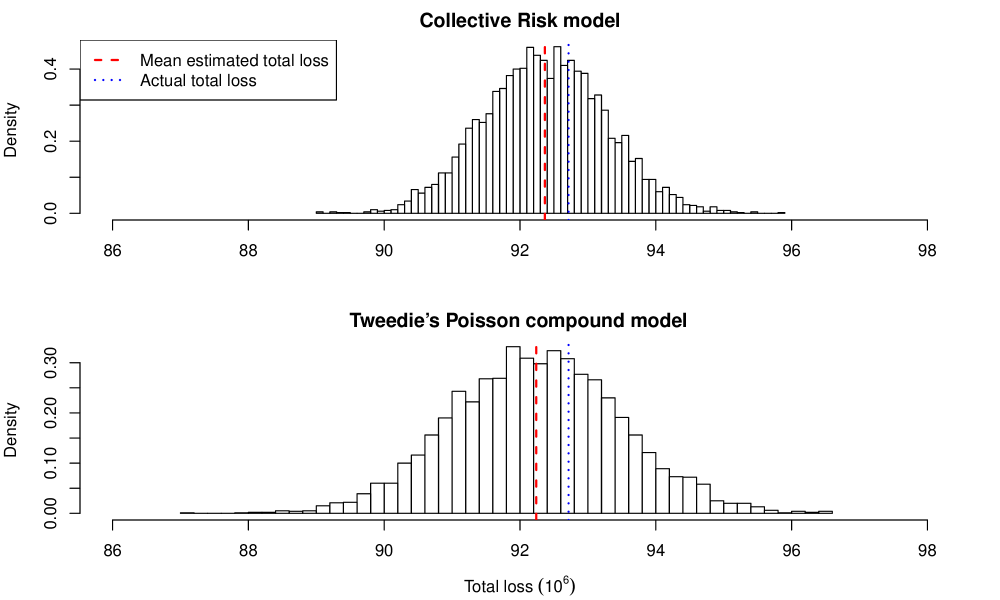
Figure 4: Predictive distribution of the total aggregated losses from the hold-out sample

9 Conclusion

We propose copula-based dependent collective risk models that allow the dependence between frequency and individual severities and that among individual severities to be separate. We also provide the conditions for the two correlation matrices used to describe the dependence to be positive definite. In particular, we emphasize that using the Gaussian copula or t-copula has computational advantages because they allow an analytic form for the conditional distribution of frequency given the individual severities.

Various extensions of our proposed models are possible as future research topics. First, it would be interesting to find appropriate general copula classes that could be used for dependent collective risk models. Although we pursue some special copulas based on computational convenience, if they cannot satisfactorily explain the given data, other complex copula functions may be necessary. Consequently, the copula choice problem (i.e., model selection problem) becomes an important issue here. Second, it would be interesting to model repeated measurements of frequency and individual severities over time. Our copula model should thus be extended to take into account the fact that the measurements from different time points are correlated. A promising approach would be to use a vine copula to combine several dependent collective risk models.

Appendix A Proofs on Covariance Matrix

Proof of Proposition 1.

Proof of (6) is a well known result from the elementary matrix algebra. For the proof of the second equation, we may use (6) and Schur complement (Zhang,, 2006).

∎

Proof of Proposition 2.

Proof of (7) is from the classical matrix algebra. For $k=0$, (8) is trivial. For $k>0$, with the following partitioned matrix representation

$$\boldsymbol{\Sigma}_{\rho_{1},\rho_{2}}^{[k,1]}=\left(\begin{array}[]{cc}1&\rho_{1}\left({\bf 1}_{k}\right)^{\mathrm{T}}\\ \rho_{1}{\bf 1}_{k}&\boldsymbol{\Sigma}_{\rho_{2}}^{[k,1]}\\ \end{array}\right)$$

and Schur complement (Zhang,, 2006), we have

$$\left(\boldsymbol{\Sigma}_{\rho_{1},\rho_{2}}^{[k,1]}\right)^{-1}=\left(\begin{array}[]{cc}1+\left(\rho_{1}\boldsymbol{I}_{k}\right)\boldsymbol{E}^{-1}\left(\rho_{1}\boldsymbol{I}_{k}\right)^{\mathrm{T}}&-\left(\rho_{1}\boldsymbol{I}_{k}\right)^{\mathrm{T}}\boldsymbol{E}^{-1}\\ -\boldsymbol{E}^{-1}\left(\rho_{1}\boldsymbol{I}_{k}\right)&\boldsymbol{E}^{-1}\\ \end{array}\right)$$ (33)

where

$$\boldsymbol{E}:=\boldsymbol{\Sigma}_{\rho_{2}}^{[k,1]}-\left(\rho_{1}\boldsymbol{I}_{k}\right)\left(\rho_{1}\boldsymbol{I}_{k}\right)^{\mathrm{T}}.$$

Furthermore, using (7), we have

$$\boldsymbol{E}^{-1}=\frac{1}{1-\rho_{2}}\left[\boldsymbol{I}_{k}-\frac{\rho_{2}-\rho_{1}^{2}}{1+(k-1)\rho_{2}-k\rho_{1}^{2}}\boldsymbol{J}_{k\times k}\right]$$ (34)

where the non-singularity of $\boldsymbol{E}^{-1}$ is guaranteed by ${\rm det}\left(\boldsymbol{\Sigma}_{\rho_{1},\rho_{2}}^{[k,1]}\right)\neq 0$. Hence, simple algebraic manipulations using (33) and (34) conclude the proof.

∎

Proof of Theorem 1.

The first part is the classical result in matrix algebra. Now, we move to the second part. Since the proof is trivial for $k=0$ or $1$, we only consider a positive integer $k>1$. By Schur complement (Zhang,, 2013), we have that $\boldsymbol{\Sigma}_{\rho_{1},\rho_{2}}^{[k,1]}$ is positive definite if and only if

$$1-\left(\rho_{1}\boldsymbol{1}_{k}\right)^{\mathrm{T}}\left(\boldsymbol{\Sigma}_{\rho_{2}}^{[k,1]}\right)^{-1}\left(\rho_{1}\boldsymbol{1}_{k}\right)$$ (35)

and

$$\boldsymbol{\Sigma}_{\rho_{2}}^{[k,1]}$$ (36)

are positive definite.

From the following calculation

$$-\left(1-\rho_{2}\right)\left(1+(k-1)\rho_{2}\right)\left(1-\left(\rho_{1}\boldsymbol{1}_{k}\right)^{\mathrm{T}}\left(\boldsymbol{\Sigma}_{\rho_{2}}^{[k,1]}\right)^{-1}\left(\rho_{1}\boldsymbol{1}_{k}\right)\right)=(1-\rho_{2})\left(k\rho_{1}^{2}-1-(k-1)\rho_{2}\right),$$

we have (35) is positive definite if and only if (10) holds. Furthermore, since (36) is positive definite if and only if (9) holds, we have that $\boldsymbol{\Sigma}_{\rho_{1},\rho_{2}}^{[k,1]}$ is positive definite if and only if (10) and (9) holds. Now, we conclude the proof by observing the intersection of (10) and (9) is (10).

∎

Proof of Proposition 3.

The first equation is well known in the classical matrix algebra, and the second equation is from the first equation and Schur complement (Zhang,, 2006). ∎

Proof of Theorem 2.

The first part is the classical result in matrix algebra. Now, we move to the second part. Since the proof is trivial for $k=0$ or $1$, we only consider a positive integer $k>1$.

By Schur complement (Zhang,, 2013), we have that $\boldsymbol{\Sigma}_{\rho_{1},\rho_{2}}^{[k,2]}$ is positive definite if and only if

$$1-\left(\rho_{1}\boldsymbol{1}_{k}\right)^{\mathrm{T}}\left(\boldsymbol{\Sigma}_{\rho_{2}}^{[k,2]}\right)^{-1}\left(\rho_{1}\boldsymbol{1}_{k}\right)$$ (37)

and

$$\boldsymbol{\Sigma}_{\rho_{2}}^{[k,2]}$$ (38)

are positive definite, where (38) is positive definite from the first part.

From the following calculation

$$-\left(1-\rho_{2}^{2}\right)\left(1-\left(\rho_{1}\boldsymbol{1}_{k}\right)^{\mathrm{T}}\left(\boldsymbol{\Sigma}_{\rho_{2}}^{[k,2]}\right)^{-1}\left(\rho_{1}\boldsymbol{1}_{k}\right)\right)=\rho_{2}^{2}\left((k-2)\rho_{1}^{2}+1\right)-2(k-1)\rho_{1}^{2}\rho_{2}+(k\rho_{1}^{2}-1),$$

we have that (37) is positive definite if and only if

$$\rho_{2}^{2}\left((k-2)\rho_{1}^{2}+1\right)-2(k-1)\rho_{1}^{2}\rho_{2}+(k\rho_{1}^{2}-1)<0.$$ (39)

Since (39) is evident for $k=2$, it is enough to prove (39) for a positive integer $k>2$. From the following observation

$$-1<\frac{(k-2)\rho_{1}^{2}+\rho_{1}^{2}}{(k-2)\rho_{1}^{2}+1}<1$$

and the fact that the left side of inequality in (39) is a quadratic equation for $k>2$, we have (39) if and only if

$$g(\rho_{1},\rho_{2},k)<0,\quad\hbox{for}\quad\rho_{2}=-1,\quad 1,\quad\frac{(k-2)\rho_{1}^{2}+\rho_{1}^{2}}{(k-2)\rho_{1}^{2}+1}$$ (40)

where

$$g(\rho_{1},\rho_{2},k):=\rho_{2}^{2}\left((k-2)\rho_{1}^{2}+1\right)-2(k-1)\rho_{1}^{2}\rho_{2}+(k\rho_{1}^{2}-1).$$

Based on this, (40) always holds.

∎

Appendix B Auxilary Results on the Dependent Collective Risk Model

For the proof of the Lemma 1, the following classical results on the conditional distribution in multivariate normal distribution are applied to the special covariance structure $\boldsymbol{\Sigma}_{\rho_{1},\rho_{2}}^{[k,1]}$.

Lemma 3.

Let $k_{0}\in\mathbb{N}_{+}$, and consider $\rho_{1},\rho_{2}\in(-1,1)$ satisfying (19) and (18) for $z=1$ and $z=2$, respectively. If we consider $\left(Y_{0},Y_{1},\cdots,Y_{k}\right){{}^{\mathrm{T}}}\sim{\rm MVN}\left(\boldsymbol{0}_{k+1},\boldsymbol{\Sigma}_{\rho_{1},\rho_{2}}^{[k,z]}\right)$ with positive integer $k\leq k_{0}$ and for $z\in\{1,2\}$, the conditional distribution of $Y_{0}$ for given $(Y_{1},\cdots,Y_{k})=(y_{1},\cdots,y_{k})$ is

$$Y_{0}\big{|}(Y_{1},\cdots,Y_{k})=(y_{1},\cdots,y_{k})\sim{\rm N}(\mu_{1},\sigma_{1}^{2})$$

where

$$\mu_{1}=\left(\rho_{1}\boldsymbol{1}_{n}^{\mathrm{T}}\right)\left(\boldsymbol{\Sigma}_{\rho_{2}}^{[k,z]}\right)^{-1}(y_{1},\cdots,y_{k})^{\mathrm{T}}\quad\hbox{and}\quad\sigma_{1}^{2}=1-\left(\rho_{1}\boldsymbol{1}_{k}^{\mathrm{T}}\right)\left(\boldsymbol{\Sigma}_{\rho_{2}}^{[k,z]}\right)^{-1}\left(\rho_{1}\boldsymbol{1}_{k}\right).$$

For the proof, see Johnson and Wichern, (2007).

Lemma 4.

Consider Conditional Model 2 for for $z\in\{1,2\}$. The conditional distribution of $N$ is given as

$${\mathbb{P}}\left(N\leq n\big{|}\boldsymbol{y}^{[k]}\right)=\Phi\left(\frac{\Phi^{-1}(F_{1}(n))-\mu_{[k,1]}}{\sigma_{[k,1]}}\right)$$

for a positive integer $k$ and $\boldsymbol{y}^{[k]}\in\mathbb{R}_{+}^{k}$, where $\mu_{[k,z]}$ and $\sigma_{[k,z]}$ are defined in (22) and (23).

Proof.

For convenience, define

$$\mathcal{I}_{N}:=\{n\in\mathcal{N}_{0}\big{|}{\mathbb{P}}\left(N=n\right)>0\}.$$

For the calculation of

$${\mathbb{P}}\left(N\leq n\big{|}y_{1},\cdots,y_{k}\right)$$

let $N^{*}\sim F_{1}^{*}$ be continuous cumulative distribution satisfying

$$F_{1}^{*}(-1)=0\quad\hbox{and}\quad F_{1}^{*}(n)=F_{1}(n)$$

for positive integer $n\in\mathcal{I}_{N}$ where $F_{1}^{*}(\cdot)$ being a strictly increasing function on $(-1,N_{\sup})$, where $N_{\sup}$ is defined as the essential supremum of $N$. Existence of such $F_{1}^{*}$ is guaranteed by linear interpolation on the fixed points

$$\{(-1,0)\}\cup\{(n,F_{1}(n))\big{|}n\in\mathcal{I}_{N}\}.$$

Now, consider the joint distribution function of $N^{*}$ and $\boldsymbol{Y}^{[k]}$

$${\mathbb{P}}\left((N^{*},Y_{1},\cdots,Y_{k})\leq(n,y_{1},\cdots,y_{k})\right):=C_{\boldsymbol{\Sigma}_{\rho_{1},\rho_{2}}^{[k,1]}}(F_{1}^{*}(n),F_{2}(y_{1}),\cdots,F_{2}(y_{k}))$$

for any integer $n$ and $(y_{1},\cdots,y_{k})\in\mathbb{R}^{k}$. Then, from Lemma 3, we have

$$\left(\Phi^{-1}(F_{1}^{*}(N^{*})),\Phi^{-1}(F_{2}(Y_{1})),\cdots,\Phi^{-1}(F_{2}(Y_{k}))\right)\sim{\rm MVN}\left(\boldsymbol{0}_{z+1},\boldsymbol{\Sigma}_{\rho_{1},\rho_{2}}^{(z)}\right)$$

and

$$\Phi^{-1}(F_{1}^{*}(N^{*}))\big{|}Y_{1}=y_{1},\cdots,Y_{k}=y_{k}\sim{\rm N}(\mu_{[k,1]},(\sigma_{[k,1]})^{2})$$

where $\mu_{[k,1]}$ and $\sigma_{[k,1]}$ are defined in (22) and (23).

Hence, we have

$${\mathbb{P}}\left(N\leq n\big{|}\boldsymbol{y}^{[k]}\right) =\frac{\frac{\partial^{z}}{\partial y_{1}\cdots,\partial y_{k}}C_{\boldsymbol{\Sigma}_{\rho_{1},\rho_{2}}^{[k_{2}]}}\left(F_{1}(n),F_{2}(y_{1}),\cdots,F_{2}(y_{k})\right)}{f_{\boldsymbol{Y}}(\boldsymbol{y}^{[k]})}$$ (41)

$$=\frac{\frac{\partial^{z}}{\partial y_{1}\cdots,\partial y_{k}}C_{\boldsymbol{\Sigma}_{\rho_{1},\rho_{2}}^{[k_{2}]}}\left(F_{1}^{*}(n),F_{2}(y_{1}),\cdots,F_{2}(y_{k})\right)}{f_{\boldsymbol{Y}}(\boldsymbol{y}^{[k]})}$$

$$={\mathbb{P}}\left(N^{*}\leq n\big{|}\boldsymbol{y}^{[k]}\right)$$

$$={\mathbb{P}}\left(\frac{\Phi^{-1}(F_{1}^{*}(N^{*}))-\mu_{[k,1]}}{\sigma_{[k,1]}}\leq\frac{\Phi^{-1}(F_{1}^{*}(n))-\mu_{[k,1]}}{\sigma_{[k,1]}}{\bigg{|}\boldsymbol{y}^{[k]}}\right)$$

$$=\Phi\left(\frac{\Phi^{-1}(F_{1}^{*}(n))-\mu_{[k,1]}}{\sigma_{[k,1]}}\right)$$

$$=\Phi\left(\frac{\Phi^{-1}(F_{1}(n))-\mu_{[k,1]}}{\sigma_{[k,1]}}\right).$$

for an integer $n\in\mathcal{I}_{N}\cup\{-1\}$. Finally, the following observation with (41)

$${\mathbb{P}}\left(N\leq n\big{|}\boldsymbol{y}^{[k]}\right)={\mathbb{P}}\left(N\leq n-1\big{|}\boldsymbol{y}^{[k]}\right)\quad\hbox{for positive integer $n\notin\mathcal{I}_{N}\cup\{-1\}$ }$$

concludes the proof. ∎

Proof of Lemma 1.

We start from the proof of part i. First, for $z=0$, we have

$$h_{N,\boldsymbol{Y}^{[k]}}(n,\boldsymbol{y}^{[k]})=f_{1}(0)$$

by definition in Conditional Model 2.

Now, let $z$ be any positive integer. Then, the joint density function of the discrete margin $N$ and the continuous margins $Y_{1},\cdots,Y_{k}$ is given by

$$h_{N,\boldsymbol{Y}^{[k]}}(n,\boldsymbol{y}^{[k]}):={\rm P}_{k}\left(n,\boldsymbol{y}^{[k]}\right)-{\rm P}_{k}\left(n-1,\boldsymbol{y}^{[k]}\right)$$

for integer $n\in\mathbb{Z}$ and $\boldsymbol{y}^{[k]}\in\mathbb{R}^{k}$, where

$${\rm P}_{k}\left(n,y_{1},\cdots,y_{k}\right):=\frac{\partial^{z}}{\partial y_{1}\cdots,\partial y_{k}}{\mathbb{P}}\left(N\leq n,Y_{1}\leq y_{1},\cdots,Y_{k}\leq y_{k}\right).$$

Here, ${\rm P}_{k}\left(n,y_{1},\cdots,y_{k}\right)$ can be written as

$${\rm P}_{k}\left(n,\boldsymbol{y}^{[k]}\right)={\mathbb{P}}\left(N\leq n\big{|}y_{1},\cdots,y_{k}\right)f_{\boldsymbol{Y}^{[k]}}(y_{1},\cdots,y_{k})$$ (42)

where $f_{\boldsymbol{Y}^{[k]}}$ is the density function of $\boldsymbol{Y}^{[k]}$. Using Lemma 4, we have

$$h_{N,\boldsymbol{Y}^{[k]}}(n,\boldsymbol{y}^{[k]}) ={\mathbb{P}}\left(N\leq n\big{|}\boldsymbol{y}^{[k]}\right)f_{\boldsymbol{Y}}(\boldsymbol{y}^{[k]})-{\mathbb{P}}\left(N\leq n-1\big{|}\boldsymbol{y}^{[k]}\right)f_{\boldsymbol{Y}}(\boldsymbol{y}^{[k]})$$

$$=f_{\boldsymbol{Y}^{[k]}}(\boldsymbol{y}^{[k]})\left(\Phi\left(\frac{\Phi^{-1}(F_{1}(n))-\mu_{[k,1]}}{\sigma_{[k,1]}}\right)-\Phi\left(\frac{\Phi^{-1}(F_{1}(n-1))-\mu_{[k,1]}}{\sigma_{[k,1]}}\right)\right)$$

for an integer $n\in\mathbb{Z}$ and $\boldsymbol{y}^{[k]}\in\mathbb{R}^{k}$.

Note that since a continuous random vector $\boldsymbol{Y}^{[k]}$ follows

$$\boldsymbol{Y}^{[k]}\sim C_{\boldsymbol{\Sigma}_{\rho_{2}}^{(z)}}(F_{2},\cdots,F_{2})$$

for any positive integer $z$, then the density function of $\boldsymbol{y}^{[k]}$ is given as in (21). The proof of Part i is complete. For brevity, we omit the proof of Part ii because it is trivial from Part i. ∎

Lemma 5.

Consider the frequency and severities

$$(N,\boldsymbol{Y}_{N}):=\begin{cases}(N,Y_{1},\cdots,Y_{N}),&N\geq 1;\\ 0,&N=0;\\ \end{cases}$$

in a dependent collective risk model in Model 1 with the assumptions employed in Conditional Model 2 or Conditional Model 3. Then, for a positive integer $n$ and $k$ satisfying $k\leq n$, we have

$${\mathbb{E}}\left[Y_{k}\big{|}N=n\right]{\mathbb{P}}\left(N=n\big{|}N>0\right)=\int_{0}^{\infty}y\,h_{N^{+},\boldsymbol{Y}^{[1]}}(n,y){\rm d}y$$ (43)

and

$${\mathbb{E}}\left[S\big{|}N=n\right]{\mathbb{P}}\left(N=n\big{|}N>0\right)=n\int_{0}^{\infty}yh_{N^{+},\boldsymbol{Y}^{[1]}}(n,y){\rm d}y$$ (44)

where $h_{N^{+},\boldsymbol{Y}^{[1]}}$ is defined in (20) or (27), depending on Conditional Model 2 or Conditional Model 3 assumptions as well as the type of the covariance matrix.

Proof.

For a positive integer $n$ and $k$ satisfying $k\leq n$, we have

$${\mathbb{E}}\left[Y_{k}\big{|}N=n\right]{\mathbb{P}}\left(N=n\big{|}N>0\right) ={\mathbb{E}}\left[Y_{k}\big{|}R=1,N^{+}=n\right]{\mathbb{P}}\left(R=1,N^{+}=n\big{|}R=1\right)$$

$$={\mathbb{E}}\left[Y_{k}\big{|}R=1,N^{+}=n\right]{\mathbb{P}}\left(N^{+}=n\big{|}R=1\right)$$

$$={\mathbb{E}}\left[Y_{k}\big{|}N^{+}=n\right]{\mathbb{P}}\left(N^{+}=n\right)$$

$$=\int_{0}^{\infty}y\,h_{N^{+},\boldsymbol{Y}^{[1]}}(n,y){\rm d}y$$

where the third equality is from the independence assumption between $R$ and $(N^{+},Y_{1},\cdots,Y_{k})$ for any positive integer $k$ satisfying $k<n_{\sup}+1$, and the last equality is from Lemma 1. Finally, the equation (43) derives

$${\mathbb{E}}\left[S\big{|}N=n\right]{\mathbb{P}}\left(N=n\big{|}N>0\right) =\sum\limits_{j=1}^{n}{\mathbb{E}}\left[Y_{j}\big{|}N=n\right]{\mathbb{P}}\left(N=n\big{|}N>0\right)$$

$$=n\int_{0}^{\infty}y\,h_{N^{+},\boldsymbol{Y}^{[1]}}(n,y){\rm d}y.$$

∎

Appendix C Proofs on Proposition 5

Proof.

The proof of the first part is from the following equation

$${\mathbb{E}}\left[S\right] ={\mathbb{E}}\left[{\mathbb{E}}\left[S\big{|}N\right]\right]$$

$$=\sum\limits_{n=0}^{\infty}{\mathbb{E}}\left[S\big{|}N=n\right]{\mathbb{P}}\left(N=n\right)$$

$$=\sum\limits_{n=1}^{\infty}{\mathbb{E}}\left[S\big{|}N=n\right]{\mathbb{P}}\left(N=n\right)$$

$$=\sum\limits_{n=1}^{\infty}{\mathbb{E}}\left[S\big{|}N=n\right]{\mathbb{P}}\left(N^{+}=n,R=1\right)$$

$$=p\sum\limits_{n=1}^{\infty}{\mathbb{E}}\left[S\big{|}N=n\right]{\mathbb{P}}\left(N=n\big{|}N>0\right)$$

$$=p\sum\limits_{n=1}^{\infty}n\int_{0}^{\infty}y\,h_{N^{+},\boldsymbol{Y}^{[1]}}(n,y){\rm d}y.$$

where the last equality is from (44). The proof of the second part follows from the following equation

$${\mathbb{E}}\left[NS\right] ={\mathbb{E}}\left[{\mathbb{E}}\left[NS\big{|}N\right]\right]$$

$$={\mathbb{E}}\left[N{\mathbb{E}}\left[S\big{|}N\right]\right]$$

$$=\sum\limits_{n=1}^{\infty}n{\mathbb{E}}\left[S\big{|}N=n\right]{\mathbb{P}}\left(N=n\right)$$

$$=p\sum\limits_{n=1}^{\infty}n{\mathbb{E}}\left[S\big{|}N=n\right]{\mathbb{P}}\left(N=n\big{|}N>0\right)$$

$$=p\sum\limits_{n=1}^{\infty}n^{2}\int_{0}^{\infty}yh_{N^{+},\boldsymbol{Y}^{[1]}}(n,y){\rm d}y$$

where the last equality is from (44).

Finally, the proof of the second part is from the following observations:

$${\mathbb{E}}\left[NM\big{|}N>0\right] ={\mathbb{E}}\left[S\big{|}N>0\right]$$

$$=\sum\limits_{n=1}^{\infty}{\mathbb{E}}\left[S\big{|}N>0,N=n\right]{\mathbb{P}}\left(N=n\big{|}N>0\right)$$

$$=\sum\limits_{n=1}^{\infty}{\mathbb{E}}\left[S\big{|}N=n\right]{\mathbb{P}}\left(N=n\big{|}N>0\right)$$

$$=\sum\limits_{n=1}^{\infty}n\int_{0}^{\infty}yh_{N^{+},\boldsymbol{Y}^{[1]}}(n,y){\rm d}y$$

where the last equality is from (44) and

$${\mathbb{E}}\left[M\big{|}N>0\right] ={\mathbb{E}}\left[\frac{1}{N}\sum\limits_{j=1}^{N}Y_{j}\big{|}N>0\right]$$

$$=\sum\limits_{n=1}^{\infty}\frac{1}{n}\sum\limits_{j=1}^{n}{\mathbb{E}}\left[Y_{j}\big{|}N>0,N=n\right]{\mathbb{P}}\left(N=n\big{|}N>0\right)$$

$$=\sum\limits_{n=1}^{\infty}\frac{1}{n}\sum\limits_{j=1}^{n}{\mathbb{E}}\left[Y_{j}\big{|}N=n\right]{\mathbb{P}}\left(N=n\big{|}N>0\right)$$

$$=\sum\limits_{n=1}^{\infty}\frac{1}{n}\sum\limits_{j=1}^{n}\int_{0}^{\infty}y\,h_{N^{+},\boldsymbol{Y}^{[1]}}(n,y){\rm d}y$$

$$=\sum\limits_{n=1}^{\infty}\int_{0}^{\infty}y\,h_{N^{+},\boldsymbol{Y}^{[1]}}(n,y){\rm d}y$$

where the last equality is from (43).

∎

References

- Albrecher and Teugels, (2006) Albrecher, H. and Teugels, J. L. (2006). Exponential behavior in the presence of dependence in risk theory. Journal of Applied Probability, 43(1):257–273.
- Asimit and Badescu, (2010) Asimit, A. V. and Badescu, A. L. (2010). Extremes on the discounted aggregate claims in a time dependent risk model. Scandinavian Actuarial Journal, 2010(2):93–104.
- Baumgartner et al., (2015) Baumgartner, C., Gruber, L. F., and Czado, C. (2015). Bayesian total loss estimation using shared random effects. Insurance: Mathematics and Economics, 62:194–201.
- Boudreault et al., (2006) Boudreault, M., Cossette, H., Landriault, D., and Marceau, E. (2006). On a risk model with dependence between interclaim arrivals and claim sizes. Scandinavian Actuarial Journal, 2006(5):265–285.
- (5) Chen, S. X. and Huang, T.-M. (2007a). Nonparametric estimation of copula functions for dependence modelling. Canadian Journal of Statistics, 35(2):265–282.
- (6) Chen, S. X. and Huang, T.-M. (2007b). Nonparametric estimation of copula functions for dependence modelling. Canadian Journal of Statistics, 35(2):265–282.
- Cossette et al., (2008) Cossette, H., Marceau, E., and Marri, F. (2008). On the compound poisson risk model with dependence based on a generalized farlie–gumbel–morgenstern copula. Insurance: Mathematics and Economics, 43(3):444–455.
- Cossette et al., (2010) Cossette, H., Marceau, E., and Marri, F. (2010). Analysis of ruin measures for the classical compound poisson risk model with dependence. Scandinavian Actuarial Journal, 2010(3):221–245.
- Cossette et al., (2018) Cossette, H., Marceau, E., and Mtalai, I. (2018). Collective risk models with dependence. Available at SSRN: https://ssrn.com/abstract=3104912 or http://dx.doi.org/10.2139/ssrn.3104912.
- Czado et al., (2012) Czado, C., Kastenmeier, R., Brechmann, E. C., and Min, A. (2012). A mixed copula model for insurance claims and claim sizes. Scand. Actuar. J., (4):278–305.
- Ferreira Jr and Minikel, (2012) Ferreira Jr, J. and Minikel, E. (2012). Measuring per mile risk for pay-as-you-drive automobile insurance. Transportation Research Record: Journal of the Transportation Research Board, (2297):97–103.
- Frees et al., (2014) Frees, E. W., Derrig, R. A., and Meyers, G. (2014). Predictive Modeling Applications in Actuarial Science, volume 1. Cambridge University Press.
- Frees et al., (2016) Frees, E. W., Lee, G., and Yang, L. (2016). Multivariate frequency-severity regression models in insurance. Risks, 4(1):4.
- Garrido et al., (2016) Garrido, J., Genest, C., and Schulz, J. (2016). Generalized linear models for dependent frequency and severity of insurance claims. Insurance: Mathematics and Economics, 70:205 – 215.
- Gijbels and Mielniczuk, (1990) Gijbels, I. and Mielniczuk, J. (1990). Estimating the density of a copula function. Communications in Statistics-Theory and Methods, 19(2):445–464.
- Hernández-Bastida et al., (2009) Hernández-Bastida, A., Fernández-Sánchez, M. P., and Gómez-Déniz, E. (2009). The net Bayes premium with dependence between the risk profiles. Insurance Math. Econom., 45(2):247–254.
- Jeong et al., (2019) Jeong, H., Valdez, E. A., Ahn, J. Y., and Park, S. (2019). Generalized linear mixed models for dependent compound risk models.
- Johnson and Wichern, (2007) Johnson, R. A. and Wichern, D. W. (2007). Applied multivariate statistical analysis. Pearson Prentice Hall, Upper Saddle River, NJ, sixth edition.
- Klugman et al., (2012) Klugman, S. A., Panjer, H. H., and Willmot, G. E. (2012). Loss models: from data to decisions, volume 715. John Wiley & Sons.
- Krämer et al., (2013) Krämer, N., Brechmann, E. C., Silvestrini, D., and Czado, C. (2013). Total loss estimation using copula-based regression models. Insurance: Mathematics and Economics, 53(3):829–839.
- Kruskal, (1958) Kruskal, W. H. (1958). Ordinal measures of association. Journal of the American Statistical Association, 53(284):814–861.
- Landriault et al., (2014) Landriault, D., Lee, W. Y., Willmot, G. E., and Woo, J.-K. (2014). A note on deficit analysis in dependency models involving coxian claim amounts. Scandinavian Actuarial Journal, 2014(5):405–423.
- Lee and Shi, (2019) Lee, G. Y. and Shi, P. (2019). A dependent frequency–severity approach to modeling longitudinal insurance claims. Insurance: Mathematics and Economics, 87:115–129.
- Lee et al., (2016) Lee, W., Park, S. C., , and Ahn, J. Y. (2016). Investigating dependence between frequency and severity via simple generalized linear models. Working Paper.
- Liu and Wang, (2017) Liu, H. and Wang, R. (2017). Collective risk models with dependence uncertainty. ASTIN Bulletin: The Journal of the IAA, 47(2):361–389.
- Nelsen, (2006) Nelsen, R. B. (2006). An introduction to copulas. Springer Series in Statistics. Springer, New York, second edition.
- Oh et al., (2019) Oh, R., Shi, P., and Ahn, J. Y. (2019). Implementation of frequency-severity association in bms ratemaking. Working Paper.
- Park et al., (2018) Park, S. C., Kim, J. H., and Ahn, J. Y. (2018). Does hunger for bonuses drive the dependence between claim frequency and severity? Insurance: Mathematics and Economics, 83:32–46.
- Shi et al., (2015) Shi, P., Feng, X., and Ivantsova, A. (2015). Dependent frequency–severity modeling of insurance claims. Insurance: Mathematics and Economics, 64:417–428.
- Sklar, (1959) Sklar, M. (1959). Fonctions de répartition à dimensions et leurs marges. Institute of Statistics of the University of Paris, 8:229–231.
- Yip and Yau, (2005) Yip, K. C. and Yau, K. K. (2005). On modeling claim frequency data in general insurance with extra zeros. Insurance: Mathematics and Economics, 36(2):153–163.
- Zhang, (2006) Zhang, F. (2006). The Schur complement and its applications, volume 4. Springer Science & Business Media.
- Zhang, (2013) Zhang, Y. (2013). Likelihood-based and bayesian methods for tweedie compound poisson linear mixed models. Statistics and Computing, 23(6):743–757.