Landau-Khalatnikov problem in relativistic hydrodynamics

Abstract

An alternative approach to solving the Landau-Khalatnikov problem on one-dimensional stage of expansion of hot hadronic matter created in collisions of high-energy particles or nuclei is suggested. Solving the relativistic hydrodynamics equations by the Riemann method yields a representation for Khalatnikov’s potential which satisfies explicitly the condition of symmetry of the matter flow with respect to reflection in the central plane of the initial distribution of matter. New exact relationships are obtained for evolution of the density of energy in the center of the distribution and for laws of motion of boundaries between the general solution and the rarefaction waves. The rapidity distributions are derived in the Landau approximation with account of the pre-exponential factor.

I Introduction

In 1950 E. Fermi supposed fermi-50 ; fermi-53 that in collisions of high-energy particles so many new elementary particles are created that their mean free path becomes much smaller than the size of the whole cloud of created nuclear (hadronic) matter. As a result, the thermal equilibrium is reached very fast and, hence, energy distribution of particles flying out of the cloud can be found with the use of statistical mechanics formulas. Soon after that, I. Ya. Pomeranchuk pomeranchuk remarked that such a matter must first expand with relativistic velocities and the real outgoing particles are formed when the temperature drops down the value about their mass. L. D. Landau showed in Ref. landau-53 that in collisions of ultra-relativistic particles the arising cloud must have a form of a thin disk due to Lorentz contraction and, consequently, the initial stage of hydrodynamic flow is mainly one-dimensional. If we denote by $2l$ the initial thickness of the disk and take the $x$-axis in the direction normal to the disk, then equations of relativistic hydrodynamics are simplified in the limit of ultra-relativistic flow velocities $v$ ($c-v\ll c$, where $c$ is the speed of light. Landau found the asymptotic solution of these equations for $\ln(t/l)\gg 1$, $\ln[(ct-x)/l]\gg 1$ with logarithmic accuracy what permitted him to make estimates of typical parameters of the flow. In the next years, the Landau theory formed a basis for theoretical description of multiple particles production in high-energy collisions of elementary particles and atomic nuclei and this approach was confirmed in experiments (see, e.g., wong ; flork ).

Exact solution of relativistic hydrodynamics equations for the one-dimensional flow was obtained by I. M. Khalatnikov in Ref. khal-54 . He formulated the problem in the following way. Let at the initial moment $t=0$ the matter be contained in the slab $-l\leq x\leq l$ and have the temperature $T_{0}\gg mc^{2}$, where $m$ is a typical mass of the matter constituents (say, of pions). For such ultra-relativistic temperatures it is natural to assume that the equation of state

$$p=\varepsilon/3,$$ (1)

takes place, where $p$ is the pressure and $\varepsilon$ is the energy density. In the case of such an equation of state the sound velocity is equal to (see LL-6 )

$$c_{s}=c\sqrt{\frac{\partial p}{\partial\varepsilon}}=\frac{c}{\sqrt{3}},$$ (2)

and it does not depend on the parameters of the medium. At the very initial stage of evolution, two self-similar rarefaction waves, centered around the points $x=\pm l$, start to propagate from the edges of the initial distribution. At the moment of time $t_{c}=l/c_{s}=\sqrt{3}\,l/c$ they collide in the center of the matter distribution at $x=0$ and after this moment the region of the general solution arises between the rarefaction waves. Thus, the general solution must satisfy the boundary conditions which correspond to matching with the rarefaction waves. Khalatnikov proved in Ref. khal-54 an important theorem that one-dimensional relativistic flow is always potential and with the use of the hodograph transform he reduced the equation for the potential to a linear second order differential equation with constant coefficients. This equation is often called in the context of relativistic hydrodynamics as Khalatnikov equation. It is equivalent mathematically to the so-called “telegraph equation” which can be solved in the case of the initial value problems with the use of the Laplace transform pb-52 . By means of skillful calculations, Khalatnikov obtained the exact solution which satisfies the necessary boundary conditions and showed that it reproduces the Landau solution in the appropriate approximation (see also bl-55 ). More detailed study of the Khalatnikov solution was later performed in other papers milekhin ; cll-74 ; wong-14 .

In spite of beauty of the Khalatnikov solution, it is represented in the form which does not demonstrate explicitly the symmetry of the flow with respect to reflection in the plane $x=0$ what hinders in some respects its investigation. Besides that, the method used in Ref. khal-54 is applicable, apparently, to the systems with constant sound velocities and it hardly can be generalized on situations when the equation for the potential in the hodograph plane has variable coefficients. In this paper, we use for solving the Landau-Khalatnikov problem the Riemann method riemann ; sommer-50 ; kgs-70 which can be applied to a wider class of equations of state. In particular, the problem of expansion of Bose-Einstein condensate released from a “box-like” trap has been solved recently in Ref. ik-19 . The found here form of the solution reflects explicitly the symmetry of the flow and with its use we have found the rapidity distribution with account of the pre-exponential factor as well as the exact expressions for the time dependence of the energy density in the center of the space distribution and the paths of the boundaries between the general solution and the rarefaction waves. Comparison of two forms of the solution demonstrates their physical equivalence.

II Relativistic hydrodynamics

From now on, to simplify formulas, we accept the system of units in which the speed of light $c$ and the initial temperature $T_{0}$ in the slab are equal to unity. At first we shall formulate the main fact from relativistic hydrodynamics to introduce the notation and necessary definitions.

II.1 Main equations

As is known LL-6 ; anile-89 , equations of relativistic hydrodynamics are contained in conservation laws of a relativistic flow which in case of a one-dimensional flow have the form

$$\frac{\partial T^{00}}{\partial t}+\frac{\partial T^{01}}{\partial x}=0,\qquad\frac{\partial T^{01}}{\partial t}+\frac{\partial T^{11}}{\partial x}=0,$$ (3)

where the components of the energy-momentum tensor $T^{\mu\nu}$ are equal to

$$\begin{split}&T^{00}=(\varepsilon+p)u^{0}u^{0}-p,\quad T^{01}=(\varepsilon+p)u^{0}u^{1},\\ &T^{11}=(\varepsilon+p)u^{1}u^{1}+p,\end{split}$$ (4)

and $u^{\mu}$ is the vector of 4-velocity

$$(u^{0},u^{1})=\left(\frac{1}{\sqrt{1-v^{2}}},\frac{v}{\sqrt{1-v^{2}}}\right)=(\cosh y,\sinh y),$$ (5)

where we have introduced the rapidity $y$ related with the flow velocity $v$ by the equation $v=\tanh y$, so that Lorentz transformation corresponds to a hyperbolic rotation by the “angle” $y$. After substitution of Eq. (5) into Eq, (4) we arrive with account of definition of the sound velocity $c_{s}^{2}=\partial p/\partial\varepsilon$ to the system of equations

$$\begin{split}&(\cosh^{2}y+c_{s}^{2}\sinh^{2}y)\frac{\partial\varepsilon}{\partial t}+2(\varepsilon+p)\sinh y\cosh y\,\frac{\partial y}{\partial t}\\ &+(1+c_{s}^{2})\sinh y\cosh y\,\frac{\partial\varepsilon}{\partial x}\\ &+(\varepsilon+p)(\sinh^{2}y+\cosh^{2}y)\frac{\partial y}{\partial x}=0,\\ &(1+c_{s}^{2})\sinh y\cosh y\,\frac{\partial\varepsilon}{\partial t}+(\varepsilon+p)(\sinh^{2}y+\cosh^{2}y)\frac{\partial y}{\partial t}\\ &+(\sinh^{2}y+c_{s}^{2}\cosh^{2}y)\frac{\partial\varepsilon}{\partial x}\\ &+2(\varepsilon+p)\sinh y\cosh y\,\frac{\partial y}{\partial x}=0.\end{split}$$

Characteristic velocities of these first order differential equations Х

$$v_{\pm}=\frac{v\pm c_{s}}{1\pm vc_{s}}$$ (6)

have clear physical meaning: speed of signal’s propagation is equal to the sum of flow velocity and the sound velocity according to the relativistic velocity addition formula and the sound can propagate downstream and upstream. One can easily find the Riemann invariants corresponding to these characteristic velocities (see, e.g., LL-6 ; anile-89 ; kamch-2000 ),

$$r_{\pm}=y\pm\int_{0}^{\varepsilon}\frac{c_{s}d\varepsilon}{\varepsilon+p},$$ (7)

which in the case of ultra-relativistic equation of state (1) reduce to

$$r_{\pm}=y\pm\sqrt{3}\,\theta,$$ (8)

where we have introduced instead of the temperature the variable $\theta=\ln T$ and took into account that Eq. (1) leads to the expression

$$\varepsilon=T^{4}$$ (9)

for the energy density. The flow velocity and the temperature as functions of the Riemann invariants are given by the formulas

$$\begin{split}&v=\tanh y=\tanh\left(\frac{r_{+}+r_{-}}{2}\right),\\ &T=e^{\theta}=\exp\left(\frac{r_{+}-r_{-}}{2\sqrt{3}}\right).\end{split}$$ (10)

Hydrodynamic equations expressed in terms of the Riemann invariants take simple diagonal form

$$\frac{\partial r_{\pm}}{\partial t}+v_{\pm}(r_{+},r_{-})\frac{\partial r_{\pm}}{\partial x}=0,$$ (11)

where the characteristic velocities

$$v_{\pm}=\frac{\tanh[(r_{+}+r_{-})/2]\pm 1/\sqrt{3}}{1\pm\tanh[(r_{+}+r_{-})/2]/\sqrt{3}}$$ (12)

are also expressed in terms of the Riemann invariants.

II.2 Rarefaction waves

Equations (11), (12) yield at once solutions for rarefaction waves. Let us consider, for example, the right edge $x=l$ of the initial distribution of the matter. Since at the initial moment of time the matter is at rest and its temperature is equal to unity, then at the initial state both Riemann invariants are equal to zero. Up to the moment $t_{c}=\sqrt{3}\,l$ of their collision, the rarefaction waves evolve independently of each other. Therefore, for example, the right rarefaction wave can depend on the parameter $l$ through the combination $x-l$ only and, consequently, the Riemann invariants in the right rarefaction wave can depend on the self-similar variable $(x-l)/t$ only. Then it follows from Eqs. (11) that one of the Riemann invariants must be constant and the variable $(x-l)/t$ must be equal to the characteristic velocity corresponding to the other Riemann invariant. In the right rarefaction wave the flow velocity is positive, that is $y>0$, and the temperature decreases during expansion of the matter, that is $\theta<0$. Hence, in the right rarefaction wave the Riemann invariant $r_{+}$ must be constant and equal to its initial value,

$$r_{+}=y+\sqrt{3}\,\theta=0.$$ (13)

Then from

$$\frac{x-l}{t}=v_{-}=\frac{v-1/\sqrt{3}}{1-v/\sqrt{3}}$$ (14)

we obtain the distribution of the flow velocity

$$v=\frac{\sqrt{3}\,(x-l)/t+1}{\sqrt{3}+(x-l)/t},$$ (15)

and from (9), (10) and (13) it is easy to find the distribution of the energy density

$$\varepsilon=\left(\frac{1-1/\sqrt{3}}{1+1/\sqrt{3}}\cdot\frac{1-(x-l)/t}{1+(x-l)/t}\right)^{\frac{2}{\sqrt{3}}}.$$ (16)

At the boundary with vacuum, where $\varepsilon\to 0$, the matter moves to the right with the speed of light, what is natural since the matter consists of particles with the thermal velocities equal in our approximation to the speed of light. Into the slab the rarefaction wave propagates with the sound velocity $(x-l)/t=-1/\sqrt{3}$ and at the boundary with the quiescent matter we have $\varepsilon=1$. In a similar way one can build the solution for the left rarefaction wave which depends on the self-similar variable $(x+l)/t$. The Riemann invariant $r_{-}=y-\sqrt{3}\,\theta=0$ is constant within it what corresponds to the negative flow velocity $y<0$.

II.3 Khalatnikov equation

After collision of the rarefaction waves at the moment $t_{c}=\sqrt{3}\,l$ in the center $x=0$ the region of the general solution appears between them, where both Riemann invariants $r_{\pm}$ change with $x$ and $t$, and finding the corresponding solution of the hydrodynamic equations is a more complicated problem than finding the rarefaction waves solutions.

Khalatnikov showed in Ref. khal-54 that one can obtain from Eqs. (3) that

$$\frac{\partial(Tu^{1})}{\partial t}+\frac{\partial(Tu^{0})}{\partial x}=0,$$ (17)

which means that we can introduce such a potential $\phi=\phi(x,t)$ that

$$d\phi=T\cosh y\cdot dt-T\sinh y\cdot dx.$$

Introducing also the light cone variables $x_{\pm}=t\pm x$ and considering the Riemann invariants $r_{\pm}$ as independent variables, we can rewrite this differential in the form

$$d\phi=A(r_{+},r_{-})dx_{-}+B(r_{+},r_{-})dx_{+},$$

where

$$\begin{split}&A(r_{+},r_{-})=\frac{1}{2}e^{\theta+y}\\ &=\frac{1}{2}\exp\left[\frac{1}{2}\left(1+\frac{1}{\sqrt{3}}\right)r_{+}+\frac{1}{2}\left(1-\frac{1}{\sqrt{3}}\right)r_{-}\right],\\ &B(r_{+},r_{-})=\frac{1}{2}e^{\theta-y}\\ &=\frac{1}{2}\exp\left[-\frac{1}{2}\left(1-\frac{1}{\sqrt{3}}\right)r_{+}-\frac{1}{2}\left(1+\frac{1}{\sqrt{3}}\right)r_{-}\right].\end{split}$$ (18)

Following Khalatnikov, we make Legendre transformation

$$W=\phi-Ax_{-}-Bx_{+},$$

where the variables $W,x_{-},x_{+}$ are considered as functions of the Riemann invariants, which corresponds to the hodograph transform known in compressible gas dynamics (see, e.g., LL-6 ; kamch-2000 ). As a result, we obtain

$$\begin{split}dW&=\frac{1}{2}\left[-\left(1+\frac{1}{\sqrt{3}}\right)Ax_{-}+\left(1-\frac{1}{\sqrt{3}}\right)Bx_{+}\right]dr_{+}\\ &+\frac{1}{2}\left[-\left(1-\frac{1}{\sqrt{3}}\right)Ax_{-}+\left(1+\frac{1}{\sqrt{3}}\right)Bx_{+}\right]dr_{-},\end{split}$$

so that

$$\begin{split}&\frac{1}{2}\left[-\left(1+\frac{1}{\sqrt{3}}\right)Ax_{-}+\left(1-\frac{1}{\sqrt{3}}\right)Bx_{+}\right]=\frac{\partial W}{\partial r_{+}},\\ &\frac{1}{2}\left[-\left(1-\frac{1}{\sqrt{3}}\right)Ax_{-}+\left(1+\frac{1}{\sqrt{3}}\right)Bx_{+}\right]=\frac{\partial W}{\partial r_{-}}.\end{split}$$

Thus, if the function $W(r_{+},r_{-})$ is found, then $x,t$ are expressed in terms of the Riemann invariants by the formulas

$$\begin{split}\begin{split}x=\sqrt{3}\,e^{-\theta}&\Big{\{}\left(\frac{\cosh y}{\sqrt{3}}+\sinh y\right)\frac{\partial W}{\partial r_{-}}\\ &+\left(\frac{\cosh y}{\sqrt{3}}-\sinh y\right)\frac{\partial W}{\partial r_{+}}\Big{\}},\\ t=\sqrt{3}\,e^{-\theta}&\Big{\{}\left(\frac{\sinh y}{\sqrt{3}}+\cosh y\right)\frac{\partial W}{\partial r_{-}}\\ &+\left(\frac{\sinh y}{\sqrt{3}}-\cosh y\right)\frac{\partial W}{\partial r_{+}}\Big{\}},\end{split}\end{split}$$ (19)

which yield the solution in implicit form.

So far we have solved formally the equation (17) by introduction of the potential $W=W(r_{+},r_{-})$. To get the equation for $W$, we can use as a second equation of relativistic hydrodynamics the entropy conservation law. If the entropy density is denoted by $\sigma$, then this law reads (see LL-6 ):

$$\frac{\partial(\sigma u^{0})}{\partial t}+\frac{\partial(\sigma u^{1})}{\partial x}=0.$$ (20)

In case of ultra-relativistic equation of state we have

$$\sigma=\frac{4}{3}T^{3}=\frac{4}{3}\exp\left[\frac{\sqrt{3}}{2}(r_{+}-r_{-})\right].$$ (21)

We multiply Eq. (20) by the Jacobian $\partial(x,t)/\partial(r_{+},r_{-})$ and with account of Eqs. (21) and (10) we obtain the equation

$$\frac{\partial^{2}W}{\partial r_{+}\partial r_{-}}-\frac{1}{2\sqrt{3}}\left(\frac{\partial W}{\partial r_{+}}-\frac{\partial W}{\partial r_{-}}\right)=0.$$ (22)

Written, instead of $r_{\pm}$, in terms of the variables $y,T$, it was obtained by Khalatnikov khal-54 . It is mathematically equivalent to the so-called “telegraph equation” which can be solved by well developed mathematical methods (see, e.g., pb-52 ; sommer-50 ; kgs-70 ). Some classes of such solutions are used in the theory of multiple particles production (see, e.g., Refs. bps-08 ; ps-11 ). In the case of the Landau-Khalatnikov problem on the slab expansion with specific boundary conditions, the Riemann method seems to be quite convenient, and we shall use it in the next section.

III Landau-Khalatnikov problem

III.1 Boundary conditions

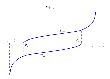
Figure 1: Plots of Riemann invariants $r_{\pm}$ as functions of $x$ at fixed moment of time $t>\sqrt{3}\,l$; $x_{L}$ and $x_{R}$ denote the boundaries of the general solution and $-l-t$ и $l+t$ denote the boundaries of the left and right rarefaction waves with vacuum.

The potential $W$, which defines the solution by the formulas (19), must satisfy Eq. (22) and the boundary conditions which follow from matching with the rarefaction waves at the corresponding edges. If Eqs. (19) are solved with respect to the derivatives $\partial W/\partial r_{\pm}$, then the solution can be written in the form

$$\begin{split}&\frac{\partial W}{\partial r_{-}}=\frac{e^{\theta}}{2}\left(\cosh y-\frac{\sinh y}{\sqrt{3}}\right)\left(x-\frac{\tanh y-1/\sqrt{3}}{1-\tanh y/\sqrt{3}}\,t\right),\\ &\frac{\partial W}{\partial r_{+}}=\frac{e^{\theta}}{2}\left(\cosh y+\frac{\sinh y}{\sqrt{3}}\right)\left(x-\frac{\tanh y+1/\sqrt{3}}{1+\tanh y/\sqrt{3}}\,t\right).\end{split}$$ (23)

Plots of the Riemann invariants as functions of the coordinate $x$ at fixed moment of time $t$ are shown in Fig. 1. The Riemann invariants $r_{+}$ and $r_{-}$ vanish at the right and left edges of the general solution, correspondingly. At these edges $x$ and $t$ satisfy the rarefaction waves solutions (see Eq. (14)), that is

$$\begin{split}&x-\frac{\tanh y-1/\sqrt{3}}{1-\tanh y/\sqrt{3}}\,t=l\quad\text{at}\quad r_{+}=0,\\ &x-\frac{\tanh y+1/\sqrt{3}}{1+\tanh y/\sqrt{3}}\,t=-l\quad\text{at}\quad r_{-}=0.\end{split}$$ (24)

Substitution of these formulas into Eqs. (23) yields the boundary conditions in the form

$$\begin{split}\left.\frac{\partial W}{\partial r_{-}}\right|_{r_{+}=0}=\frac{l}{4}&\Big{\{}\left(1-\frac{1}{\sqrt{3}}\right)e^{\frac{1}{2}\left(1-\frac{1}{\sqrt{3}}\right)r_{-}}+\\ &+\left(1+\frac{1}{\sqrt{3}}\right)e^{-\frac{1}{2}\left(1+\frac{1}{\sqrt{3}}\right)r_{-}}\Big{\}},\\ \left.\frac{\partial W}{\partial r_{+}}\right|_{r_{-}=0}=-\frac{l}{4}&\Big{\{}\left(1+\frac{1}{\sqrt{3}}\right)e^{\frac{1}{2}\left(1+\frac{1}{\sqrt{3}}\right)r_{+}}+\\ &+\left(1-\frac{1}{\sqrt{3}}\right)e^{-\frac{1}{2}\left(1-\frac{1}{\sqrt{3}}\right)r_{+}}\Big{\}},\end{split}$$ (25)

Since the potential $W$ is defined up to an additive constant, we can fix its value $W(0,0)=0$ in the origine of the hodograph plane $(r_{+},r_{-})$. Then integration of Eqs. (25) gives the final form of the boundary conditions along the boundaries between the general solution and the rarefaction waves:

$$\begin{split}&W(0,r_{-})=\frac{l}{2}e^{\frac{r_{-}}{2\sqrt{3}}}\sinh\frac{r_{-}}{2},\\ &W(r_{+},0)=-\frac{l}{2}e^{-\frac{r_{+}}{2\sqrt{3}}}\sinh\frac{r_{+}}{2}.\end{split}$$ (26)

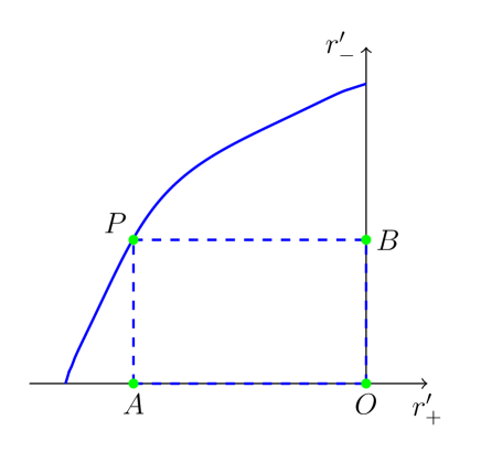
Figure 2: Plot of Riemann invariants $r_{\pm}$ in the hodograph plane $(r_{+}^{\prime},r_{-}^{\prime})$ for the general solution at a fixed moment of time.

III.2 Riemann’s method

So, we have to solve Eq. (22) with the boundary conditions (26) prescribed on the characteristics $r_{+}=0$ and $r_{-}=0$ of this equation. In his fundamental paper riemann , B. Riemann gave the following method of solving this problem. If we are interested in the value of the function $W$ at the point $P=(r_{+},r_{-})$ (see Fig. 2), then we should draw in the hodograph plane $(r_{+}^{\prime},r_{-}^{\prime})$ from the point $P$ two characteristics $PA$ $(r_{+}^{\prime}=r_{+}=\mathrm{const})$ and $PB$ $(r_{-}^{\prime}=r_{-}=\mathrm{const})$, which together with the characteristics $AO$ and $OB$ with known values of $W(r_{+}^{\prime},0)$ and $W(0,r_{-}^{\prime})$ along them form a closed contour $\mathcal{C}=PAOB$ in this plane. Since the symbols $(r_{+},r_{-})$ denote now the coordinates of the “observation point” in the hodograph plane, we have introduced the notation $(r_{+}^{\prime},r_{-}^{\prime})$ for varying along the contour $\mathcal{C}$ coordinates. We define in this plane such a vector $(V,U)$, that the integral $\int_{\mathcal{C}}(Vdr_{+}^{\prime}+Udr_{-}^{\prime})=0$ vanishes. The components $(V,U)$ depend here on the function $W$ satisfying Eq. (22) and also on another function $R=R(r_{+}^{\prime},r_{-}^{\prime};r_{+},r_{-})$ on which we can impose some appropriate conditions without changing the zero value of the above integral. Riemann showed that if one demands, first, that the function $R$ satisfies the conjugated equation which in our case reads

$$\frac{\partial^{2}R}{\partial r_{+}^{\prime}\partial r_{-}^{\prime}}+\frac{1}{2\sqrt{3}}\left(\frac{\partial R}{\partial r_{+}^{\prime}}-\frac{\partial R}{\partial r_{-}^{\prime}}\right)=0,$$ (27)

second, it satisfies the boundary conditions

$$\begin{split}&\frac{\partial R}{\partial r_{+}^{\prime}}-\frac{R}{2\sqrt{3}}=0\quad\text{along}\quad PB;\\ &\frac{\partial R}{\partial r_{-}^{\prime}}+\frac{R}{2\sqrt{3}}=0\quad\text{along}\quad PA,\end{split}$$ (28)

and, third, we fix its value at the point $P$,

$$W(r_{+},r_{-};r_{+},r_{-})=1,$$ (29)

then the value of $W$ at the point $P=(r_{+},r_{-})$ will be given by the formula

$$W(P)=\frac{1}{2}(RW)_{A}+\frac{1}{2}(RW)_{B}+\int_{A}^{O}Vdr_{+}^{\prime}+\int_{O}^{B}Udr_{-}^{\prime},$$ (30)

where $A=(r_{+},0)$, $B=(0,r_{-})$, $O=(0,0)$ and $U$, $V$ are defined in terms of the boundary values (26) by the expressions

$$\begin{split}&U=\frac{1}{2}\left({W}\frac{\partial R}{\partial r_{+}^{\prime}}-R\frac{\partial{W}}{\partial r_{+}^{\prime}}\right)-\frac{{W}R}{2\sqrt{3}},\\ &V=\frac{1}{2}\left(R\frac{\partial{W}}{\partial r_{-}^{\prime}}-{W}\frac{\partial R}{\partial r_{-}^{\prime}}\right)-\frac{{W}R}{2\sqrt{3}}.\end{split}$$ (31)

Although it seems that to solve Eq. (27) for $R$ is not easier than to solve Eq. (22) for $W$, the boundary conditions (28) are now so simple that the function $R$ can be found in our case without much difficulty. Since the equation of state (1) is similar to the non-relativistic isothermic equation of state $p=c_{s}^{2}\rho$ with constant isothermic sound velocity $c_{s}$ which does not depend on the density of gas, and the corresponding function $R$ was found by Riemann himself in Ref. riemann , we can adjust his result to our case to obtain

$$\begin{split}R(r_{+}^{\prime},r_{-}^{\prime};r_{+},r_{-})&=\exp\left[\frac{(r_{+}^{\prime}-r_{+})+(r_{-}-r_{-}^{\prime})}{2\sqrt{3}}\right]\\ &\times I_{0}\left(\sqrt{(r_{+}^{\prime}-r_{+})(r_{-}-r_{-}^{\prime})/3}\right),\end{split}$$ (32)

where $I_{0}(z)$ is the Bessel function of complex argument (see, e.g., Ref. ww ).

When we have the Riemann formula (30) with known expression (32) for the Riemann function $R$, then it is not difficult to get the expression for the potential $W$. To this end, we notice first, that substitution of (31) into (30) and elementary integration by parts cast the Riemann formula to

$$\begin{split}W(P)=&-\int_{A}^{O}R\left(\frac{\partial W}{\partial r_{+}^{\prime}}+\frac{W}{2\sqrt{3}}\right)dr_{+}^{\prime}+\\ &+\int_{O}^{B}R\left(\frac{\partial{W}}{\partial r_{-}^{\prime}}-\frac{W}{2\sqrt{3}}\right)dr_{-}^{\prime}.\end{split}$$ (33)

Then substitution of the boundary expressions (26) for $W$ yields after simple transformations

$$\begin{split}W(r_{+},r_{-})&=\frac{l}{2}\exp\left(\frac{r_{-}-r_{+}}{2\sqrt{3}}\right)\\ &\Bigg{\{}\int_{r_{+}}^{0}\left(\cosh\frac{r}{2}+\frac{2}{\sqrt{3}}\sinh\frac{r}{2}\right)e^{\frac{r}{\sqrt{3}}}\\ &\times I_{0}\left(\sqrt{\frac{(r-r_{+})r_{-}}{3}}\right)dr\\ &+\int_{0}^{r_{-}}\left(\cosh\frac{r}{2}-\frac{2}{\sqrt{3}}\sinh\frac{r}{2}\right)e^{-\frac{r}{\sqrt{3}}}\\ &\times I_{0}\left(\sqrt{\frac{-r_{+}(r_{-}-r)}{3}}\right)dr\Bigg{\}}.\end{split}$$ (34)

This formula together with Eqs. (19) defines implicitly the dependence of the Riemann invariants $r_{\pm}$ on $x$ and $t$, and with the help of Eqs. (10) we find the dependence of the physical variables on coordinate and time. The above expression for $W$ seems somewhat more complex than the corresponding expression for the potential in Khalatnikov’s solution khal-54 (see below Section 4), but it is invariant with respect to the transformation $r_{+}\to-r_{-}$, $r_{-}\to-r_{+}$, which corresponds to the change of the sign of the flow velocity which means the symmetry of the flow with respect to reflection in the plane $x=0$. Such a symmetry is absent in Khalatnikov’s expression for the potential. Let us infer some consequences from the obtained solution.

III.3 Initial stage of evolution of the general solution region

For small time $t-t_{c}\ll t_{c}$ after the collision moment $t_{c}=l\sqrt{3}$ of the rarefaction waves, the absolute values of the Riemann invariants $r_{\pm}$ are also small and we can use the series expansions of the derivatives of $W(r_{+},r_{-})$,

$$\begin{split}&\frac{\partial W}{\partial r_{+}}\approx l\left(-\frac{1}{2}-\frac{r_{+}+r_{-}}{2\sqrt{3}}-\frac{r_{+}^{2}}{8}\right),\\ &\frac{\partial W}{\partial r_{-}}\approx l\left(\frac{1}{2}-\frac{r_{+}+r_{-}}{2\sqrt{3}}+\frac{r_{-}^{2}}{8}\right).\end{split}$$ (35)

Then Eqs. (19) yield the series expansions

$$\begin{split}x\approx&l(r_{+}+r_{-})\left(\frac{1}{2\sqrt{3}}-\frac{5(r_{+}-r_{-})}{24}\right),\\ t\approx&l\Big{(}\sqrt{3}+\frac{r_{-}-r_{+}}{2}+\frac{\sqrt{3}}{8}(r_{+}^{2}+r_{-}^{2})-\\ &-\frac{r_{+}r_{-}}{2\sqrt{3}}\Big{)},\qquad|r_{+}|,r_{-}\ll 1.\end{split}$$ (36)

At $t=l\sqrt{3}$ we have $r_{+}=r_{-}=0$, as it should be, and during further evolution we always have $r_{+}=-r_{-}$ at $x=0$ (see Fig. 1).

At the right boundary between the general solution and the rarefaction wave, the invariant $r_{+}$ vanishes and substitution of $r_{+}=0$ yields the law of motion of this boundary in a parametric form,

$$\begin{split}x_{R}\approx&lr\left(\frac{1}{2\sqrt{3}}+\frac{5r}{24}\right),\\ t\approx&l\Big{(}\sqrt{3}+\frac{r}{2}+\frac{\sqrt{3}}{8}r^{2}\Big{)},\qquad r\ll 1,\end{split}$$ (37)

that is, with the same accuracy,

$$\begin{split}x_{R}(t)\approx&l\left\{\frac{t}{l\sqrt{3}}-1-4\left(\frac{t}{l\sqrt{3}}-1\right)^{2}\right\},\\ &\frac{t}{l\sqrt{3}}-1\ll 1.\end{split}$$ (38)

Thus, at the initial stage this boundary propagates with the sound velocity.

In the center of matter distribution with $r_{-}=-r_{+}\equiv r$ we obtain $t\approx l(\sqrt{3}+r+(\sqrt{3}/12)r^{2})$, so that the temperature at this point decreases with time according to the formula

$$\begin{split}T=&e^{-\frac{r}{\sqrt{3}}}\approx 1-\left(\frac{t}{l\sqrt{3}}-1\right)+\frac{3}{4}\left(\frac{t}{l\sqrt{3}}-1\right)^{2},\\ &\frac{t}{l\sqrt{3}}-1\ll 1.\end{split}$$ (39)

III.4 Motion of boundaries of the general solution

Since the flow is symmetric with respect to the plane $x=0$, it is enough to consider the motion of the right boundary only $x_{R}(t)$ where $r_{+}=0$. At this point the value of $\left.\partial W/\partial r_{-}\right|_{r_{+}=0}$ is already known from the boundary condition (25) and a similar limit for $\partial W/\partial r_{+}$ can be easily found, so that we get $(r=r_{-})$

$$\begin{split}&\left.\frac{\partial W}{\partial r_{+}}\right|_{r_{+}=0}=\frac{l}{2}e^{-\frac{r}{2\sqrt{3}}}\left(\cosh\frac{r}{2}+\frac{1}{\sqrt{3}}\sinh\frac{r}{2}-2e^{\frac{r}{\sqrt{3}}}\right),\\ &\left.\frac{\partial W}{\partial r_{-}}\right|_{r_{+}=0}=\frac{l}{2}e^{-\frac{r}{2\sqrt{3}}}\left(\cosh\frac{r}{2}-\frac{1}{\sqrt{3}}\sinh\frac{r}{2}\right).\end{split}$$ (40)

Substitution of these formulas into Eqs. (19) yields the parametric form for the law of motion of the right boundary,

$$\begin{split}&x_{R}=l\left\{1+e^{\frac{r}{\sqrt{3}}}\left(\sqrt{3}\,\sinh\frac{r}{2}-\cosh\frac{r}{2}\right)\right\},\\ &t=le^{\frac{r}{\sqrt{3}}}\left(\sqrt{3}\,\cosh\frac{r}{2}-\sinh\frac{r}{2}\right).\end{split}$$ (41)

For small $r\ll 1$ these formulas reproduce, naturally, Eqs. (37), and for asymptotically large time $t/l\gg 1$, when $r\gg 1$, we obtain

$$x\approx l+t-l(\sqrt{3}+1)\left(\frac{2}{\sqrt{3}-1}\cdot\frac{t}{l}\right)^{\frac{2-\sqrt{3}}{2+\sqrt{3}}},\qquad t\gg l.$$ (42)

As we see, this boundary propagates with velocity close to the light speed and it lags behind the edge $x=t$ at the distance growing with time. However, the ralative size of the region occupied by the rarefaction wave decreases with time. It is easy to write down analogous formulas for motion of the left boundary. The paths of edges of the right rarefaction wave and the general solution are shown in Fig. 3.

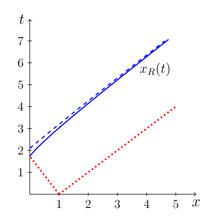
Figure 3: The solid line shows the motion of the right boundary $x_{R}(t)$ according to the exact formulas (41) with $l=1$, whereas the dashed line according to the asymptotic formula (42). Dotted lines depict the paths of the rarefaction wave edges: its right edge propagates into vacuum with the light speed and the left edge into the initial matter distribution with the sound speed $1/\sqrt{3}$ till the collision moment with the left rarefaction wave in the center at $x=0$.

It is natural to study the time dependence of the energy density at the edge of the general solution as a function of a proper time $\overline{t}$ on the clock moving with this edge,

$$\begin{split}\overline{t}=\int_{\sqrt{3}\,l}^{t}dt\sqrt{1-v^{2}}&=\int_{0}^{r}\frac{dt/dr}{\cosh(r/2)}dr\\ &\approx l\cdot\frac{\sqrt{3}+1}{2}\exp\left(\frac{r}{\sqrt{3}}\right),\end{split}$$ (43)

where $t=t(r)$ is expressed by the second formula (41). The parameter $r$ equals to $r=-2\sqrt{3}\,\theta$ and, consequently, the energy density $\varepsilon=T^{4}=e^{4\theta}$ drops down with growth of the proper time as

$$\varepsilon\approx\left(1+\frac{\sqrt{3}}{2}\right)\cdot\left(\frac{l}{\overline{t}}\right)^{2}.$$ (44)

III.5 Evolution of the energy density in the center of the distribution

In the center of the matter distribution at $x=0$, where $r_{-}=-r_{+}\equiv r$, the second formula (19) yields after simple transformations

$$\begin{split}t=l\sqrt{3}\,e^{\frac{r}{\sqrt{3}}}\frac{d}{dr}&\Big{\{}e^{\frac{r}{\sqrt{3}}}\int_{0}^{r}\left(\cosh\frac{r^{\prime}}{2}-\frac{1}{\sqrt{3}}\sinh\frac{r^{\prime}}{2}\right)\\ &\times e^{-\frac{r^{\prime}}{\sqrt{3}}}I_{0}\left(\sqrt{\frac{r(r-r^{\prime})}{3}}\right)dr^{\prime}\Big{\}},\end{split}$$ (45)

what determines the dependence of the parameter $r$ on time $t$. Since here $T=e^{\theta}=e^{-r/\sqrt{3}}$, we find thus the time dependence of the temperature and of the energy density in the center. At asymptotically large time, when $t\gg l$ and $r\gg 1$, we take into account that the integral in Eq. (45) converges at $r^{\prime}\sim 1$ due to the exponential factor $\exp(-r^{\prime}/\sqrt{3})$ in the integrand and therefore we can use the asymptotic approximation (see Ref. ww )

$$I_{0}(z)\approx\frac{e^{z}}{\sqrt{2\pi z}},$$ (46)

for the Bessel function, so that

$$I_{0}\left(\sqrt{\frac{r(r-r^{\prime})}{3}}\right)\approx\frac{e^{\frac{r}{\sqrt{3}}}\cdot e^{-\frac{r^{\prime}}{2\sqrt{3}}}}{\sqrt{2\pi r/\sqrt{3}}},\qquad r\gg r^{\prime}\sim 1,$$ (47)

and replace the upper limit of integration by infinity. As a result, we obtain

$$t\approx l\,\sqrt{\frac{2}{3\pi(-\theta)}}e^{-3\theta},\qquad|\theta|\gg 1.$$ (48)

This equation can be solved with respect to ${-\theta}$ with logarithmic accuracy and we get

$$-\theta\approx\frac{1}{3}\ln\left(\frac{t}{l}\right),$$

that is

$$T\approx\left(\frac{2}{\pi\ln(t/l)}\right)^{1/6}\left(\frac{l}{t}\right)^{1/3},$$ (49)

which means that the energy density decreases with time as

$$\varepsilon=T^{4}\approx\frac{1}{(2\pi\ln(t/l))^{2/3}}\cdot\left(\frac{2l}{t}\right)^{4/3},\qquad t\gg l.$$ (50)

The law $\varepsilon\sim(l/t)^{4/3}$ was obtained by Landau landau-53 in the approximation in which the logarithmically dependent on time factors are neglected.

III.6 Flow far from the boundaries of the general solution with rarefaction waves

At large time the temperature of matter decreases very much compared with its initial value, hence $|\theta|=|\ln T|\gg 1$. If we are interested in properties of flow far from the edges of the general solution, where one of the Riemann invariants vanishes, then we can assume that absolute values of both Riemann invariants $r_{\pm}=y\pm\sqrt{3}\theta$ are large and use the asymptotic formula (46) for calculation of integrals in Eq. (34) replacing again the limits of integration by $r_{+}\to-\infty$, $r_{-}\to\infty$. As a result, we arrive at a simple formula for $W$,

$$\begin{split}W(r_{+},r_{-})\approx&l\cdot 3^{3/4}\sqrt{\frac{2}{\pi}}\frac{(-r_{+}r_{-})^{1/4}}{r_{-}-r_{+}+4\sqrt{-r_{+}r_{-}}}\\ &\times\exp\left[\frac{(\sqrt{r_{-}}+\sqrt{-r_{+}})^{2}}{2\sqrt{3}}\right].\end{split}$$ (51)

If the pre-exponential factor is omitted, then we return to the solution obtained by Landau landau-53 ; bl-55 . For calulation of derivatives of this expression it is enough in the main approximation to differentiate the exponent only, since then the order of the pre-exponential factor does not decrease,

$$\begin{split}\frac{\partial W}{\partial r_{+}}\approx&-l\frac{3^{1/4}}{\sqrt{2{\pi}}}\cdot\left(\frac{r_{-}}{-r_{+}}\right)^{1/4}\frac{\sqrt{r_{-}}+\sqrt{-r_{+}}}{r_{-}-r_{+}+4\sqrt{-r_{+}r_{-}}}\\ &\times\exp\left[\frac{(\sqrt{r_{-}}+\sqrt{-r_{+}})^{2}}{2\sqrt{3}}\right],\\ \frac{\partial W}{\partial r_{-}}\approx&l\frac{3^{1/4}}{\sqrt{2{\pi}}}\cdot\left(\frac{-r_{+}}{r_{-}}\right)^{1/4}\frac{\sqrt{r_{-}}+\sqrt{-r_{+}}}{r_{-}-r_{+}+4\sqrt{-r_{+}r_{-}}}\\ &\times\exp\left[\frac{(\sqrt{r_{-}}+\sqrt{-r_{+}})^{2}}{2\sqrt{3}}\right].\end{split}$$ (52)

Substitution of these formulas into Eqs. (19) determines implicitly the dependence of the Riemann invariants on $x$ and $t$. The Riemann invariants change within the intervals

$$\begin{split}&-r_{m}\lesssim r_{+}\lesssim 0,\qquad 0\lesssim r_{-}\lesssim r_{m},\\ &r_{m}\approx\frac{2+\sqrt{3}}{2\sqrt{3}}\ln\left(\frac{2}{\sqrt{3}-1}\cdot\frac{t}{l}\right),\end{split}$$ (53)

as it can be found from the second formula (41). If we fix time $t$ and choose some value of, say, $r_{+}$ in this interval, then the corresponding value of $r_{-}$ can be found from the second equation (19) and the corresponding value of $x$ is determined by the first formula (19). Thus, we can find the values of the Riemann invariants at fixed $t$ as functions of $x$ which determines the distributions of the physical parameters according to Eqs. (10). The general character of the flow was determined in Refs. landau-53 ; bl-55 , where it was shown that the energy is concentrated in the ultra-relativistic regions of the flow whereas the particles are located mainly in the region of relatively small velocities. We shall not discuss all that in any details and notice only that now the distributions can be calculated with account of the pre-exponential factor. Typical distribution of the energy density is shown in Fig. 4. Time of evolution $t=1000$ is chosen large to make the Landau approximation accurate enough with values of the Riemann invariants about $r_{\pm}\sim 5$. However, for not too much values of time the role of the pre-exponential factor becomes more important which can be noticed in experimentally measured rapidity distributions of resulting particles.

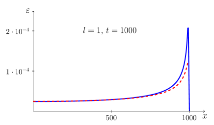
Figure 4: Distribution of the energy density $\varepsilon(x)$ on $x>0$ at $t=1000$ for $l=1$ is shown by a solid line for asymptotic solution (51) complemented by the rarefaction wave. Dashed line corresponds to the Landau approximation with the pre-exponential factor in Eq. (51) replaced by a constant chosen in such a way that both distributions coincide at $x=0$.

III.7 Distributions on rapidities

Experimentally measured quantity is the distribution of particles on the rapidity $y$ (see, e.g., bearden-05 ) which is usually compared with the Gauss formula corresponding to the Landau approximation. Here we derive more accurate formula with account of the pre-exponential factor.

According to Landau landau-53 , distributions of particle density coincides with entropy distributions. Therefore, the rapidity distribution is proportional to the entropy distribution of each fluid matter particle at the moment of its transition into real hadrons at the temperature of the order of their mass milekhin . In the proper reference frame of the fluid particle amount of the entropy in the small layer with thickness $dx^{\prime}$ is equal to $\sigma dx^{\prime}=\sigma(u^{0})^{\prime}\cdot dx^{\prime}$, where $(u^{0})^{\prime}=1$ is the time-component of the 4-velocity. This expression can be considered as a product of the entropy flux by the space component of the 4-vector $dx^{i}$. In Minkowski geometry, the quantity $(u^{0})^{\prime}dx^{\prime}$ is an “area” element $A^{\prime 01}=(u^{0})^{\prime}dx^{\prime}-(u^{1})^{\prime}dt^{\prime}$, where $(u^{1})^{\prime}=0$ in the proper reference frame of the fluid particle. This tensor component is invariant with respect to Lorentz transformation and, hence, we obtain the expression for the differential of entropy in an arbitrary reference frame as

$$dS=\sigma(u^{0}dx-u^{1}dt).$$ (54)

In the center of inertia reference frame the coordinates $t$ and $x$ are related with the parameters $\theta$, $y$ by the formulas

$$\begin{split}t=e^{-\theta}\left(\sinh y\frac{\partial W}{\partial y}-\cosh y\frac{\partial W}{\partial\theta}\right),\\ x=e^{-\theta}\left(\cosh y\frac{\partial W}{\partial y}-\sinh y\frac{\partial W}{\partial\theta}\right),\end{split}$$ (55)

which are obtained from Eqs. (19) by means of the replacements (8). Their substitution into Eq. (54) with account of $\sigma\propto T^{3}=e^{3\theta}$, $u^{0}=\cosh y$, $u^{1}=\sinh y$ yields

$$dS\propto e^{2\theta}\left\{\left(\frac{\partial^{2}W}{\partial y^{2}}-\frac{\partial W}{\partial\theta}\right)dy+\left(\frac{\partial^{2}W}{\partial\theta\partial y}-\frac{\partial W}{\partial y}\right)d\theta\right\}.$$

At the moment of formation of real particles one can neglect the change of temperature and to get for distribution of particles on their rapidities the expression

$$dN\propto dS\propto e^{2\theta}\left(\frac{\partial^{2}W}{\partial y^{2}}-\frac{\partial W}{\partial\theta}\right)dy,$$

where $dN$ is the number of particles with rapidities within the interval $(y,y+dy)$. In the asymptotic region far from the boundaries along which $y=\pm\sqrt{3}\,\theta$, a simple calculation yields

$$\begin{split}dN=&G(-\theta)\cdot\frac{\theta-\sqrt{\theta^{2}-y^{2}/3}}{(\theta^{2}-y^{2}/3)^{1/4}(\theta-2\sqrt{\theta^{2}-y^{2}/3})}\\ &\times\exp\left[\theta+\sqrt{\theta^{2}-\frac{y^{2}}{3}}\right]dy,\end{split}$$ (56)

where $G(-\theta)$ is a normalization factor defined by the condition $\int_{\sqrt{3}\theta}^{-\sqrt{3}\theta}dN=1$ and $\theta=\ln T$ corresponds to the temperature of transformation of hadronic matter to separate particles. In fact, the dependence of $G(-\theta)$ on $-\theta$ is very weak and it changes from the value $G(3)\approx 0.3597$ to its limiting value $G(\infty)=(1/2)\sqrt{3/(2\pi)}\approx 0.3455$ by 4% only. For $-\theta\gg 1$, $y\ll|\theta|$ this distribution becomes Gaussian one,

$$dN=\frac{1}{\sqrt{6\pi(-\theta)}}\exp\left(-\frac{y^{2}}{6(-\theta)}\right)dy,$$ (57)

in agreement with the experiment at very large collision energy bearden-05 . For more moderate energy of collision it may be necessary to use more accurate formula (56).

IV Comparison with the solution in Khalatnikov’s form

I. M. Khalatnikov used in Ref. khal-54 the reference frame with the right edge of the initial distribution located at the point $x=0$ (rather than at $x=0$ as we do). However, the relationships (55) between the coordinates $x,t$ and parameters $\theta,y$ were used without translation transformation $x\to x-l$. As a result, the expression obtained for the potential,

$$\widetilde{W}(\theta,y)=l\sqrt{3}\,e^{\theta}\int_{y/\sqrt{3}}^{-\theta}e^{2z}I_{0}\left(\sqrt{z^{2}-y^{2}/3}\right)dz,$$ (58)

is not invariant with repect to change of the sign of the flow velocity $y\to-y$, but it has simpler form compared with our expression (34). Written in terms of the Riemann invariants, the Khalatnikov solution takes the form

$$\begin{split}&\widetilde{W}(r_{+},r_{-})=l\sqrt{3}\,e^{\frac{r_{+}-r_{-}}{2\sqrt{3}}}\times\\ &\times\int_{\frac{r_{-}+r_{+}}{2\sqrt{3}}}^{\frac{r_{-}-r_{+}}{2\sqrt{3}}}e^{2z}I_{0}\left(\sqrt{z^{2}-\frac{(r_{+}-r_{-})^{2}}{12}}\right)dz.\end{split}$$ (59)

It is evident that the functions $W$ in (34) and $\widetilde{W}$ in (59) do not coincide with each other, since they have different symmetry properties. But, of course, their physical consequences are the same. For example, at the right boundary between the general solution and the rarefaction wave at $y=-\sqrt{3}\,\theta$ we find the derivatives

$$\left.\frac{\partial\widetilde{W}}{\partial y}\right|_{y=-\sqrt{3}\,\theta}=-le^{-\theta},\quad\left.\frac{\partial\widetilde{W}}{\partial\theta}\right|_{y=-\sqrt{3}\,\theta}=-l\sqrt{3}\,e^{-\theta},$$

and their substitution into Eq, (55) gives the law of motion of this boundary coinciding with Eq. (41) after taking into account the translational shift of the origine of the coordinate system to the point $x=l$. At the center of the matter distribution, where $y=0$, Eq. (58) gives the expression ($r=-\sqrt{3}\,\theta$)

$$t=l\sqrt{3}\left\{e^{\frac{2r}{\sqrt{3}}}I_{0}\left(\frac{r}{\sqrt{3}}\right)-\int_{0}^{\frac{r}{\sqrt{3}}}e^{2z}I_{0}(z)dz\right\},$$ (60)

which seems different from Eq. (45), but the coincidence of the two expressions can be easily checked numerically.

It is worth noticing that one cannot calculate the pre-exponential factor by a simple substitution of the asymptotic formula (46) into Eq. (59) since now there is no factors in the integrand function which provides convergence of the integral at finite $z$. Thus, each form of the solution has its own advantages in studying the flow in this problem.

V Conclusion

In this paper, we have obtained a new form of solution of the Landau-Khalatnikov problem about expansion of a slab of matter in the relativistic hydrodynamics. This problem was formulated first by Landau landau-53 and he got its asymptotic solution. The Riemann method riemann ; sommer-50 applied to the Khalatnikov equation khal-54 allows one to get the solution which satisfies the necessary boundary condition at the boundaries with the rarefaction waves and represents explicitly the symmetry of the flow. Although this solution is physically equivalent to the Khalatnikov solution, its mathematical form has some advantages and permits one to obtain the asymptotic solution with account of the pre-exponential factor. We have performed quite detailed study of parameters of the flow at all stages of its evolution.

References

- (1) E. Fermi, High Energy Nuclear Events, Progr. Theor. Phys., 5, 570-583 (1950).
- (2) E. Fermi, Angular Distribution of the Pions Produced in High Energy Nuclear Collisions, Phys. Rev., 81, 683 (195).
- (3) I. Ya. Pomeranchuk, On the theory of particles production in a single event, Dokl. Akad. Nauk USSR, 78, 889 (1951) (in Russian).
- (4) L. D. Landau, On multiple production of particles during collisions of fast particles, Izv. Akad. Nauk USSR, ser. fiz., 17, 51 (1953) (in Russian) [L. D. Landau, Collected Papers, p. 569, Gordon and Breech, N. Y., 1965].
- (5) C.-Y. Wong, Introduction to High-Energy Heavy-Ion Collisions, World Scientific, Singapore, (1994).
- (6) W. Florkowski, Phenomenology of Ultra-Relativistic Heavy-Ion Collisions, World Scientific, Singapore, (2010).
- (7) I. M. Khalatnikov, Some questions of relativistic hydrodynamics, Zh. Eksp. Teor. Fiz., 27, 529-541 (1954) (in Russian).
- (8) L. D. Landau and E. M. Lifshitz, Fluid Mechanics, Pergamon, Oxford, (1959).
- (9) B. van der Pol and H. Bremmer, Operational Calculus Based on the Two-Sided Laplace Integral, Cambridge Univ., Cambridge, (1950).
- (10) S. Z. Belenkij and L. D. Landau, A hydrodynamic theory of multiple formation of particles, Usp. Fiz. Nauk, 56, 309-348 (1955) (in Russian) [L. D. Landau, Collected Papers, p. 665, Gordon and Breech, N. Y., 1965].
- (11) G. A. Milekhin, A hydrodynamic theory of multiple production of particles in collisions of fast nucleons with nuclei, Zh. Eksp. Teor. Fiz., 35, 1185-1197 (1958) (in Russian).
- (12) S. Chadha, C. S. Lam, and Y. C. Leung, Proton-proton collisions in the hydrodynamic theory, Phys. Rev. D 10, 2817 (1974).
- (13) C.-Y. Wong, A. Sen, J. Gerhard, G. Torrieri, and K. Read, Analytical solutions of Landau (1+1)-dimensional hydrodynamics, Phys. Rev. C 90, 064907 (2014).
- (14) B. Riemann, Über die Fortpflanzung ebener Luftwellen von endlicher Schwingungsweite, Abh. Ges. Wiss. Göttingen, Math.-phys. Kl., 8, 43 (1860).
- (15) A. Sommerfeld, Partial Differential Equations in Physics, Lectures on Theoretical Physics Vol. VI, Academic, New York, (1964).
- (16) N. S. Koshlyakov, E. B. Gliner, M. M. Smirnov, Partial Differential Equations of Mathematical Physics, Vysshaya shkola, Moscow (1970) (in Russian).
- (17) S. K. Ivanov, A. M. Kamchatnov, Collision of rarefaction waves in Bose-Einstein condensates, Phys. Rev., A 99, 013609 (2019).
- (18) A. M. Anile, Relativistic Fluids and Magneto-Fluids, Cambridge University Press, N. Y., (1989).
- (19) A. M. Kamchatnov, Nonlinear Periodic Waves and Their Modulations, World Scientific, Singapore (2000).
- (20) G. Beuf, R. Peschanski, E. N. Saridakis, Entropy flow of a perfect fluid in (1+1) hydrodynamics, Phys. Rev. C 78, 064509 (2008).
- (21) R. Peschanski, E. N. Saridakis, Exact (1+1)-dimensional flows of perfect fluid, Nucl. Phys., A 849, 147-164 (2011).
- (22) E. T. Whittaker and D. N. Watson, A Course of Modern Analysis, Cambridge Univ., Cambridge, (1927).
- (23) J. G. Bearden et al. (BRAHMS Collaboration), Charged Meson Rapidity Distributions in Central Au+Au collisions at GeV, Phys. Rev. Lett., 94, 162301 (2005).