Partial Server Pooling in Redundancy Systems

Abstract

Partial sharing allows providers to possibly pool a fraction of their resources when full pooling is not beneficial to them. Recent work in systems without sharing has shown that redundancy can improve performance considerably. In this paper, we combine partial sharing and redundancy by developing partial sharing models for providers operating multi-server systems with redundancy. Two M/M/N queues with redundant service models are considered. Copies of an arriving job are placed in the queues of servers that can serve the job. Partial sharing models for cancel-on-complete and cancel-on-start redundancy models are developed. For cancel-on-complete, it is shown that the Pareto efficient region is the full pooling configuration. For a cancel-on-start policy, we conjecture that the Pareto frontier is always non-empty and is such that at least one of the two providers is sharing all of its resources. For this system, using bargaining theory the sharing configuration that the providers may use is determined. Mean response time and probability of waiting are the performance metrics considered.

I Introduction

We consider resource sharing by service systems modeled as multi server queueing systems, e.g., server farms, cloud computing systems, call centers, inventory systems, and emergency services. These services dimension their resources (e.g., number of servers) to provide a prescribed quality of service (QoS). Two commonly used QoS measures in delay systems (as opposed to loss systems) are the probability of waiting for service (famously characterized by the Erlang-C formula for M/M/N queues), and waiting and/or sojourn time moments.

For many of the above mentioned systems, resources are expensive and different independent systems could possibly share their resources to improve their customers’ QoS. It may also be that procurement of additional resources takes time, and sharing could be a useful interim measure. In [10], two models for resource sharing among different service providers are identified. (1) Providers pool their existing resources with the expectation that the joint system is beneficial over operating alone. (2) Providers jointly determine the total resources for the QoS requirements of the combined system. For both systems, cooperative game theory is used to determine the cost shares among the coalition of providers.

Our interest in this paper is related to the first kind of system above, but in the setting of non-transferable utility. In this case, the providers may not always have the incentive to completely pool their resources, as the following example illustrates. Consider two service providers, 1 and 2, modeled as $M/M/N$ queues. The providers have, respectively, 20 and 30 servers and an offered load of, respectively, 16 and 28 Erlangs. When operating alone, the providers’ QoS, measured as Erlang-C probabilities, are, respectively, 0.25 and 0.62. When the providers merge to create a coalition system of 50 servers with 44 Erlangs load, the QoS in the joint system is 0.28. Clearly, the first provider is not incentivized to join the ‘naive’ full pooling coalition. A natural question then is to seek partial pooling models that may incentivize both providers to join the coalition. Here by partial pooling models we mean that each provider contributes a fraction (could be all) of its resources into a common pool which can then be used to serve requests from any provider.

The focus of this work is to develop partial sharing models in delay systems and answer two key questions: How to share? How much to share? We consider delay systems where arriving jobs are replicated into queues at the servers that can serve them. Sending redundant copies of a job to queues at servers that can service them is of interest due to their use in several systems like call centers and cloud server farms. Two redundancy models are popular—cancel-on-complete and cancel-on-start. Analytical studies of these models without partial sharing are available, among others, [6, 4, 2].

The rest of the paper is organized as follows: In the next section, we describe our system model involving two providers operating multi-server service systems, and present our redundancy-based partial sharing mechanism. In Section III, we analyze partial sharing for cancel-on-complete systems. Exploiting recent results of [4], we show that full sharing is the only Pareto-optimal configuration. In Section IV, we consider partial sharing in the cancel-on-start system. We obtain the stationary distributions of the number in the system, and for a special case, we show that the Pareto region is such that at least one of the providers shares all of its resources. Based on numerical evidence, we conjecture that this is true in general. We then use bargaining theory to capture the stable sharing agreement. We conclude in Section V by showing that the results of cancel-on-complete are directly applicable to the joint system that uses a single server (capacity equal to sum of server capacities of the two systems) with two queues served according to a balanced fair rate allocation. We also discuss related literature on resource pooling and future work.

II System Model

Consider two service providers $P_{1}$ and $P_{2}$ with $N_{1}$ and $N_{2}$ servers, respectively. The servers are homogenous with unit service rate. Jobs of provider $P_{i}$ arrive according to a Poisson process of rate $\lambda_{i}$, and the service requirements (a.k.a. sizes) of jobs are i.i.d. exponential with mean $1/\nu_{i}<\infty.$ $\rho_{i}:=\lambda_{i}/\nu_{i}$ denotes the traffic load $P_{i}.$

Each server has its own queue, and serves jobs using FCFS discipline. Both providers use redundancy as follows. When a job arrives, $d$ copies (a.k.a. replicas) of this job are sent to $d$ different servers. Further, both providers replicate copies to all servers that can process their jobs. In the standalone system, this implies that $d=N_{i}$ for provider $i.$ On the other hand, in a pooled system, $d_{i}$ can be larger than $N_{i}$ and depends on the number of servers shared by the other provider $-i.$

Two types of redundancy models are commonly studied in the literature. The redundant copies of a job can either be removed from the system at the instance when first of its copies starts service, i.e., cancel-on-start ($\mathsf{c.o.s.}$) replication, or at the instance when first of its copies finishes its service, i.e., cancel-on-complete ($\mathsf{c.o.c.}$) replication. We analyze both $\mathsf{c.o.s.}$ as well as $\mathsf{c.o.c.}$ policies in the next two sections.

For stability, we assume $\rho_{i}<N_{i}$ for $i=1,2.$ This condition is necessary and sufficient for both $\mathsf{c.o.c.}$ and $\mathsf{c.o.s.}$ when the arrival process is Poisson and replica sizes are i.i.d. with an exponential distribution (see [4] for $\mathsf{c.o.c.}$ and [2] for $\mathsf{c.o.s.}$).

We shall consider two different performance metrics for the service providers: (i) the stationary waiting probability, defined as the steady state probability that an arriving job has to wait for service; and (ii) the stationary mean response time. We make the following important remark at this point.

Remark 1.

Since each server has its own waiting line, strictly speaking, the standalone systems are not Erlang-C systems. However, the $\mathsf{c.o.s.}$ system in which copies are replicated to all the servers is indeed equivalent to an Erlang-C system [2]. It thus makes sense to refer to the waiting probability in the standalone $\mathsf{c.o.s.}$ system as the Erlang-C probability.

In light of the above remark, the performance metrics of the Erlang-C system will serve as another benchmark when highlighting the benefits of partial sharing compared to the no sharing case. For provider $P_{i},$ the standalone Erlang-C probability $C_{i}^{\text{s}}$ and the stationary mean response time $D_{i}^{\text{s}}$ are given by

$$C_{i}^{\text{s}}=\frac{\rho_{i}^{N_{i}}}{\rho_{i}^{N_{i}}+{\big{(}1-\frac{\rho_{i}}{N_{i}}\big{)}\left(\sum\limits_{k=0}^{N_{i}-1}\frac{\rho_{i}^{k}}{k!}\right)N_{i}!}},\ D_{i}^{\text{s}}=\frac{1}{\nu_{i}}+\frac{C_{i}^{\text{s}}}{\nu_{i}(N_{i}-\rho_{i})}.$$

II-A Partial Sharing Policy

We propose a partial resource sharing policy, where each of the providers contributes some of its servers to a common pool. The servers in this common pool can serve the jobs from both of the service providers. Hence the system has three types of servers depending on the types of jobs they can serve. We now formally define the partial sharing policy.

The partial sharing policy is parametrized by $(k_{1},k_{2}),$ where $k_{i}\in\{0,1,2,\dots,N_{i}\}$ is the number of servers contributed by provider $P_{i}$ to the common pool. Hence these $N_{1}+N_{2}$ servers are classified in the following three separate pools.

• Dedicated servers of provider $P_{1}$: $N_{1}-k_{1}$ dedicated servers which can serve only jobs of provider $P_{1}$.

• Dedicated servers of provider $P_{2}$: $N_{2}-k_{2}$ dedicated servers which can serve only jobs of provider $P_{2}.$

• Common pool: $k_{1}+k_{2}$ shared servers which can serve jobs from both providers $P_{1}$ and $P_{2}$.

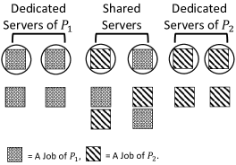
Figure 1: Partial sharing policy

On arrival of a provider $i$ job into the system, copies of this job are sent to all the $N_{i}+k_{-i}$ servers that can serve it, i.e., to the $N_{i}-k_{i}$ dedicated servers of provider $P_{i}$ and $k_{1}+k_{2}$ servers in the shared pool.

Notations: For a partial sharing configuration $(k_{1},k_{2})$, for provider $P_{i}$, the waiting probability is denoted by $C_{i}(k_{1},k_{2})$ and the mean response time will be denoted by $D_{i}(k_{1},k_{2})$. To keep the notation simple, we shall use the same notation for the two performance metrics in both the $\mathsf{c.o.c.}$ as well as the $\mathsf{c.o.s.}$ systems. Since these two systems are treated in separate sections, no confusion should arise.

II-B Pareto-frontier

Each provider is assumed to be optimizing its own performance metrics, i.e., for a provider to consider sharing its servers, it has to benefit from doing so. To determine which partial sharing policy will be acceptable to the providers, we use the concept of Pareto-frontier which is widely used in economics and multi-objective optimization.

Let $B_{i}$ be either $C_{i}$ or $D_{i}$. A policy/configuration $(k_{1},k_{2})$ is said to be Pareto-optimal, if,

1. $B_{i}(k_{1},k_{2})<B_{i}(0,0)$ for $i=1,2,$ and

2. there does not exist another policy $(l_{1},l_{2})$ such that $B_{i}(l_{1},l_{2})\leq B_{i}(k_{1},k_{2}),$ for $i=1,2,$ with strict inequality for at least one $i$.

That is, a Pareto-optimal configuration is one that results in improved performance for each provider, and for which there does not exist any other policy that is better for both the providers. The Pareto-frontier, $\mathcal{P}$ is defined as the set of all Pareto optimal policies and is the set of policies for which both providers benefit individually compared to policies outside this set. Within the set, two policies are not comparable since one provider gains while the other loses. Existence of a non-empty $\mathcal{P}$ implies that partial sharing can benefit both providers when compared to not sharing. In the next two sections, we show that $\mathcal{P}$ is indeed non-empty for both $\mathsf{c.o.c.}$ and $\mathsf{c.o.s.}$ systems.

III Partial pooling via cancel-on-complete replication

In this section, we explore partial pooling via the resource sharing mechanism described in Section II with cancel-on-complete ($\mathsf{c.o.c.}$) replication. Specifically, each incoming job of provider $i$ releases a replica of the job to all eligible servers (the $N_{i}-k_{i}$ servers in the dedicated pool of $P_{i}$, and the $k_{1}+k_{2}$ servers in the common pool) upon arrival. The sizes of these replicas are assumed to be i.i.d. and exponentially distributed with mean $1/\nu_{i}$ (we comment on this assumption later). The job gets completed when the first of its replicas completes service, at which point the remaining replicas are cancelled.

Our main result is that under $\mathsf{c.o.c.}$ replication, complete pooling (i.e., $k_{i}=N_{i}\ \forall\ i$) is the only Pareto-optimal partial sharing configuration between the providers for the mean response time metric. In other words, full pooling is not just optimal for overall system performance, but also individually optimal from the standpoint of each provider. Thus, complete pooling is the only reasonable configuration that the providers would agree upon in a bargaining setting. In contrast, under cancel-on-start replication (discussed in Section IV), the Pareto-frontier is a continuum of partial sharing configurations, which may not include the complete pooling configuration.

In the following, we first obtain, by invoking recent results by Bonald et al. (see [4]), an expression for the steady state mean response time under our partial pooling model with $\mathsf{c.o.c.}$ replication. This enables us to characterize certain monotonicity properties of the mean response time in the sharing parameters. Finally, using these monotonicity properties, we determine the Pareto-frontier of sharing configurations.

TABLE I: Comparison of mean response time for the case $N_{1}=N_{2}=N,$ the standalone waiting probabilities of $S_{1}$ and $S_{2}$ without replication being 5% and 10%, respectively and $\nu_{1}=\nu_{2}=1$.

$N$	$D_{1}$		$D_{2}$		$D_{1}=D_{2}=D$
	Standalone system	Standalone system	Standalone system	Standalone system	Full Sharing	Naive
	with c.o.c. replication	without replication	with c.o.c. replication	without replication	with c.o.c.	Full Sharing
5	0.3231	1.0161	0.3722	1.0372	0.1730	1.0220
10	0.2121	1.0106	0.2491	1.0249	0.1145	1.0015
15	0.1679	1.0084	0.1988	1.0199	0.0910	1.0012
20	0.1428	1.0071	0.1699	1.0170	0.0776	1.0011

III-A Performance characterization under $\mathsf{c.o.c.}$ replication

In [4], Bonald et al. establish an equivalence between the distribution of the steady state system occupancy vector in a multiclass $\mathsf{c.o.c.}$ queueing system, and that in a single server system with balanced fair scheduling. Specifically, for a given partial sharing configuration $(k_{1},k_{2}),$ consider the following two systems.

$\boldsymbol{\mathcal{S}1}$: $\mathcal{S}1$ is a multiclass queueing system with two classes (corresponding to the two providers) and $N_{1}+N_{2}$ servers. The servers are identical and have a unit service rate. Jobs of class $i$ (i.e., corresponding to Provider $i$) can be served on the $N_{i}-k_{i}$ dedicated servers of provider $i$ as well as on the $k_{1}+k_{2}$ servers in the common pool. An incoming job is replicated on all eligible servers in $\mathsf{c.o.c.}$ mode.

$\boldsymbol{\mathcal{S}2}$: $\mathcal{S}2$ is a two-class single server system. The two job classes correspond to the two providers, and the system maintains a separate queue for the active jobs of either class. The server has a service rate of $N_{1}+N_{2}.$ Let $n_{i}$ denote the number of jobs of class $i$ in the system. For a given system state $(n_{1},n_{2}),$ each class $i$ is allotted a service rate $r_{i},$ where $(r_{1},r_{2})$ is the balanced fair rate allocation corresponding to the polymatroidal rate region $\mathcal{R}(k_{1},k_{2})$ defined as follows:

$$\mathcal{R}(k_{1},k_{2}) =\{(r_{1},r_{2})\in\mathbb{R}_{+}^{2}:\ r_{1}\leq N_{1}+k_{2},\;$$

$$\qquad r_{2}\leq N_{2}+k_{1},\;r_{1}+r_{2}\leq N_{1}+N_{2}\}.$$

The above rate region is also depicted in Figure 2. We refer the reader to [5] for a detailed description of balanced fair scheduling. Proposition 1 in [4] shows that the steady state average system occupancies in $\mathcal{S}1$ and $\mathcal{S}2$ coincide. From this equivalence, and using known results for the steady state mean response times under balanced fair scheduling (see [5]), one obtains the following characterization of the mean response time for our partial pooling model under $\mathsf{c.o.c.}$ replication.

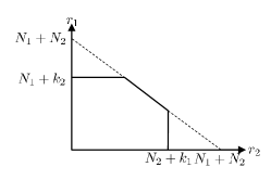
Figure 2: Rate region $\mathcal{R}(k_{1},k_{2})$ for BF-based partial pooling

Lemma 1.

For partial sharing configuration $(k_{1},k_{2})$ with $\mathsf{c.o.c.}$ replication, the steady state mean response time corresponding to jobs of provider $i$, denoted $D_{i}(k_{1},k_{2})$ is given by $D_{i}(k_{1},k_{2})=\nu_{i}^{-1}\Bigg{(}\frac{1}{N_{1}+N_{2}-\rho_{1}-\rho_{2}}+\bigg{(}\frac{\left(1-\frac{\rho_{i}}{N_{1}+N_{2}}\right)\frac{1}{N_{i}+k_{-i}}}{\left(1-\frac{\rho_{i}}{N_{i}+k_{-i}}\right)^{2}}-\frac{\frac{1}{N_{1}+N_{2}}}{1-\frac{\rho_{i}}{N_{1}+k_{2}}}\bigg{)}\left(\frac{1-\frac{\rho_{1}}{N_{1}+N_{2}}}{1-\frac{\rho_{1}}{N_{1}+k_{2}}}+\frac{1-\frac{\rho_{2}}{N_{1}+N_{2}}}{1-\frac{\rho_{2}}{N_{2}+k_{1}}}-1\right)^{-1}\Bigg{)}.$

The proof of Lemma 1 can be found in Appendix A. Given the above performance characterization, we now analyse the Pareto-frontier of partial sharing configurations.

III-B Pareto-optimal sharing configurations

We first state the following monotonicity properties of the mean response time under $\mathsf{c.o.c.}$ replication with respect to the sharing paramters $k_{1}$ and $k_{2}.$

Lemma 2.

Under $\mathsf{c.o.c.}$ replication,

1. $D_{i}(k_{1},k_{2})$ is a strictly decreasing function of $k_{-i},$

2. $D_{i}(k_{1},k_{2})$ is a strictly increasing function of $k_{i}$ when $k_{-i}<N_{-i},$

3. $D_{i}(k_{1},k_{2})$ is insensitive in $k_{i}$ when $k_{-i}=N_{-i}.$

The proof of Lemma 2 can be found in Appendix B. The first statement of the lemma states that $P_{i}$ benefits from additional servers contributed by $P_{-i}$ to the common pool. Statement (2) and (3) deal with the impact of $P_{i}$’s contribution to the common pool on its own performance. Interestingly, this dependence depends on the extent to $P_{-i}$’s contribution. When $P_{-i}$ does not contribute all its servers to the common pool (i.e., $k_{-i}<N_{-i}$), $P_{i}$’s own performance deteriorates as it contributes additional servers to the common pool. However, if $P_{-i}$ has contributes all its servers to the common pool (i.e., $k_{-i}=N_{-i}$), then $P_{i}$’s performance is insensitive to its own contribution to the common pool. This insensitivity plays a crucial role in determining the Pareto-frontier of partial sharing configurations.

Theorem 1.

Under $\mathsf{c.o.c.}$ replication, complete pooling (i.e., $k_{1}=N_{1},k_{2}=N_{2}$) is the only Pareto-optimal configuration.

Proof.

It follows from Lemma 2 that

$$D_{1}(k_{1},k_{2}) \stackrel{{\scriptstyle(a)}}{{\geq}}D_{1}(k_{1},N_{2})=D_{1}(N_{1},N_{2}),$$

$$D_{2}(k_{1},k_{2}) \stackrel{{\scriptstyle(b)}}{{\geq}}D_{2}(N_{1},k_{2})=D_{2}(N_{1},N_{2}).$$

Moreover, the inequality $(a)$ (respectively, $(b)$) is strict when $k_{1}<N_{1}$ (respectively, $k_{2}<N_{2}$). Therefore,

$$(N_{1},N_{2})=\{\arg\min D_{1}(k_{1},k_{2})\}\cap\{\arg\min D_{2}(k_{1},k_{2})\}$$

i.e., only at $k_{1}=N_{1},$ $k_{2}=N_{2}$ are both $D_{1}(k_{1},k_{2})$ and $D_{2}(k_{1},k_{2})$ minimized. Equivalently, all partial sharing configurations except the full sharing configuration will have a higher mean response time for at least one of the service providers. Therefore, the full sharing configuration i.e., $k_{1}=N_{1}$ and $k_{2}=N_{2}$ is the only Pareto-optimal configuration. ∎

From a bargaining standpoint, Theorem 1 states that complete pooling is the only mutually agreeable configuration the providers would settle upon under $\mathsf{c.o.c.}$ replication. This is in stark contrast to the case of $\mathsf{c.o.s.}$ replication (addressed in the following section), where complete pooling may not even be Pareto-optimal. Interestingly, under $\mathsf{c.o.c.}$ replication, full pooling is also a Nash equilibrium between the providers.

We conclude with a couple of remarks on $\mathsf{c.o.c.}$ replication in the context of partial pooling.

Remark 2.

When neither operator contributes to the pool, i.e., $(k_{1},k_{2})=(0,0)$, the system is not equivalent to two standalone Erlang-C systems (one for each operator). At $(0,0)$, each operator replicates copies to all of its servers. It is not hard to show that $D_{i}(0,0)<D_{i}^{s},$ where $D_{i}^{s}$ refers to the mean response time in the standalone Erlang-C system.

Remark 3.

The stationary waiting probability is not a particularly meaningful metric under $\mathsf{c.o.c.}$ replication. Indeed, $\mathsf{c.o.c.}$ replication is often used in applications where the beginning of service is hard to detect. Moreover, the power of the $\mathsf{c.o.c.}$ redundancy system depends to quite some extent on the assumptions of independent copies and exponential service time distributions. When copies are being served in parallel on several servers, these two assumptions imply that the service rate of the job is equal to the sum of the rates of the servers. It is as though the servers had pooled their service rates to serve the job. This can considerably increase the service rate for a job and hence decrease the mean response time. It could thus happen that under complete pooling, a job enters into service later than in the standalone Erlang-C system (or in a partially pooled system), but finishes service earlier. This could result in the stationary probability of wait being higher in the completely pooled system, even though the mean response time is the lowest possible.

III-C Numerical study

We now present the results from some numerical experiments to illustrate the benefits of resource pooling via $\mathsf{c.o.c.}$ replication. In Table I, we present the results for the case $N_{1}=N_{2}=N,$ with the arrival rates set so that the standalone (Erlang-C) probability of wait for $P_{1}$ and $P_{2}$ are 0.05 and 0.1, respectively. We take $\nu_{1}=\nu_{2}=1.$ Note that with complete pooling, which is the only Pareto-optimal sharing configuration, $D_{1}(N_{1},N_{2})=D_{2}(N_{1},N_{2}).$ We compare the mean response time under this Pareto-optimal configuration with the the mean response time in the standalone (Erlang-C) systems, the case $k_{1}=k_{2}=0$ (standalone $\mathsf{c.o.c.}$ replicated systems), as well as naive full pooling without replication (an Erlang-C system with $N_{1}+N_{2}$ servers, and arrival rate $\lambda_{1}+\lambda_{2}$). Note that complete resource pooling with $\mathsf{c.o.c.}$ replication results in a considerable reduction of mean response time for both providers, sometimes even by an order of magnitude.

IV Partial pooling via cancel-on-start replication

In this section, we explore partial resource pooling via cancel-on-start ($\mathsf{c.o.s.}$) replication. In this model, incoming jobs of provider $i$ get replicated at all the $N_{i}+k_{-i}$ eligible servers as before. However, as soon as the first replica begins service, the others get cancelled. Thus, under $\mathsf{c.o.s.}$ replication, only one replica actually begins service, making it more attractive in applications where parallel processing of replicas is either infeasible (as in call centers) or undesirable (e.g., because the replicas have comparable size, making parallel processing of replicas inefficient). Throughout this section, we assume that $\nu_{1}=\nu_{2}=\nu.$

Partial pooling under $\mathsf{c.o.s.}$ replication is equivalent to a hypothetical join-the-least-workload system, where each server maintains a FCFS queue, and an incoming job gets dispatched on arrival to that eligible server that has the least unfinished work. An alternative and equivalent view of our $\mathsf{c.o.s.}$-based model is the following: All jobs (from both providers) wait in a single FCFS queue, and each server processes the earliest arriving eligible job. This latter view makes our model an instance of the multi-server, multi-class system analysed by Visschers et al. in [14], for which a product-form description of the stationary distribution is available. An example of this equivalence with three servers is shown in Fig. 3.

Figure 3: Equivalence of $\mathsf{c.o.s.}$ redundancy and a single FCFS queue. The copy of a job is indicated by ^′. So, $J_{1}$ and $J_{1}^{\prime}$ are copies of the same job.

The contributions of this section are as follows.

1. We use the framework in [14] to obtain a characterization of the stationary probability of waiting as well as the stationary mean response time for each provider, under the $\mathsf{c.o.s.}$-based partial sharing model.

2. Since the expressions for the above performance metrics are fairly involved, we are only able to analytically characterize the Pareto-frontier for the stationary waiting probability metric when $N_{1}=N_{2}=1.$ In this case, by suitably extending the space of sharing configurations to $[0,1]^{2}$ via time-sharing across configurations in $\{0,1\}^{2}$, we show that Pareto-optimal sharing configurations involve at least one provider always contributing its server to the common pool (i.e., $k_{i}=1$ for some $i$). Intuitively, under efficient partial sharing configurations, the more congested provider always places its server in the common pool, whereas as the less congested provider places its server in the common pool for some (long-run) fraction of time.

3. We conjecture that the above structure of the Pareto-frontier holds for $N_{1},N_{2}\geq 1.$ This conjecture is validated via numerical evaluations.

4. Finally, we invoke the Kalai-Smorodinsky solution from bargaining theory to capture the partial sharing configuration that the providers would agree upon. Via numerical experiments, we demonstrate the potential benefits from partial resource pooling between service providers.

We begin with the following remark on the special cases of no pooling and complete pooling.

Remark 4.

The case $k_{1}=k_{2}=0$ corresponds to provider $i$ performing $\mathsf{c.o.s.}$ replication among its own $N_{i}$ servers, which is in turn equivalent to an $M/M/N_{i}$ (Erlang-C) system. Thus,

$$C_{i}(0,0)=C^{s}(\rho_{i},N_{i})\qquad(i=1,2).$$

Complete pooling corresponds to an aggregated Erlang-C, which implies that

$$C_{1}(N_{1},N_{2})=C_{2}(N_{1},N_{2})=C^{s}(\rho_{1}+\rho_{2},N_{1}+N_{2}).$$

Next, we formulate our partial pooling model with $\mathsf{c.o.s.}$ replication in the framework of [14].

IV-A Performance characterization using the framework of [14]

Let $\mathcal{M}=\{1,2,\cdots,N_{1}+N_{2}\}$ denote the set of all servers and $\{m_{1},\cdots,m_{i-1},m_{i}\}$ be the set of busy servers. The busy servers are labelled in increasing order of the arrival times of the jobs they serve; for example, $m_{1}\in\mathcal{M}$ is the label of the server processing the earliest arriving job in the system. Let $n_{j}$ denote the number of jobs that cannot be served by servers in the set $\mathcal{M}\setminus\{m_{1},\cdots,m_{j-1},m_{j}\}$. Under the formulation of [14], the state $s$ of the system is represented as

$$s=(n_{i},m_{i},\cdots,n_{2},m_{2},n_{1},m_{1}).$$

As an illustration of this state description, for the example in Fig. 3, the state of the system is $(3,S_{3},0,S_{2},0,S_{1})$. This state description is actually an aggregated one because out of the three waiting jobs two can only be served in $S_{1}$ and $S_{3}$. For a complete state description, the type of the job indicating the servers in which it could be served should also have been included. However, due to the assumption of Poisson arrivals, all the arrival streams can be aggregated into a single stream, and each arrival can be reassigned its type at the moment when a server becomes free. We refer the reader to [14] for details of this state space description.

Using this state description, under a certain assignment rate condition on how servers are selected when an arriving job finds more than one idle eligible server, [14] establishes a product form stationary distribution.

To state the assignment rate condition, we need to develop the following notation. For $\{m_{1},\cdots,m_{j-2},m_{j-1}\}\subset\mathcal{M},$ and $m_{j}\notin\{m_{1},\cdots,m_{j-2},m_{j-1}\},$ let $\lambda_{m_{j}}(m_{1},\cdots,m_{j-2},m_{j-1})$ denote the transition rate from the state $(n_{j-1},m_{j-1},\cdots,n_{1},m_{1})$ to the state $(0,m_{j},n_{j-1},m_{j-1},\cdots,n_{1},m_{1}).$ That is, $\lambda_{m_{j}}$ is the rate at which an incoming job is sent to server $m_{j}$ when servers $\{m_{1},\cdots,m_{j-2},m_{j-1}\}$ are busy and the others are idle. The assignment rate condition is the following:
Assignment Rate Condition: For $1\leq i\leq N_{1}+N_{2}$ and for every vector $(m_{1},\cdots,m_{i})$ composed of elements from $\mathcal{M},$

$$\prod_{j=1}^{i}\lambda_{m_{j}}(m_{1},\cdots,m_{j-1})=\prod_{j=1}^{i}\lambda_{m_{j}}(\tilde{m}_{1},\cdots,\tilde{m}_{j-1})$$

for every permutation $\tilde{m}_{1},\cdots,\tilde{m}_{i}$ of $m_{1},\cdots,m_{i}.$

That it is always possible to design assignment probabilities to free eligible servers such that the above condition is satisfied is proved in [14]. Let us define $\lambda(\{m_{1},\cdots,m_{i-1},m_{i}\})$ as the aggregate arrival rate corresponding to jobs which cannot be served by any server in the set $\mathcal{M}\setminus\{m_{1},\cdots,m_{i}\}$. The assignment rate condition implies the following product-form stationary distribution.

Theorem 2 (Theorem 2 in [14]).

Assuming the assignment rate condition, the steady state probability for any state $s=(n_{i},m_{i},\cdots,n_{2},m_{2},n_{1},m_{1})$ is given by:

$$\pi(s)=\alpha_{i}^{n_{i}}\cdots\alpha_{1}^{n_{1}}\frac{\Pi_{\lambda}(\{m_{1},\cdots,m_{i-1},m_{i}\})}{i!}\pi(0)$$

where,

$$\Pi_{\lambda}(\{m_{1},m_{2},\cdots,m_{i}\})=\prod_{j=1}^{i}\lambda_{m_{j}}{(\{m_{1},\cdots,m_{j-2},m_{j-1}\})}$$

$$\alpha_{i}=\frac{1}{i}\lambda(\{m_{1},\cdots,m_{i-1},m_{i}\})$$

Using this stationary distribution, one can compute the waiting probability as well as the mean response time for each partial sharing configuration $(k_{1},k_{2});$ see Appendix C. We note that while there is some simplification achieved by specializing Theorem 2 to our two-class setting with three types of servers (i.e., two dedicated pools and one common pool), the expressions for the performance metrics, while amenable to numerical computation, are too cumbersome for an analytical treatment of the Pareto-frontier.

IV-B Pareto-frontier of partial sharing configurations under $\mathsf{c.o.s.}$ for $N_{1}=N_{2}=1$

We now specialize to the case $N_{1}=N_{2}=1,$ focusing on the stationary waiting probability metric. To analyse the Pareto-frontier with $\mathsf{c.o.s.}$ replication, we need to generalize the space of sharing configurations $(k_{1},k_{2})$ to allow for real valued $k_{i}\in[0,1].$ We do this using randomization as follows. Provider $i$ contributes its server to the common pool with probability $k_{i};$ these actions being independent across providers. Of course, the above probabilities should really be interpreted as time-fractions. So the configuration $(k_{1},k_{2})$ is achieved by time-sharing between the configurations $(0,0),$ $(0,1),$ $(1,0)$ and $(1,1),$ with (long run) time-fractions $(1-k_{1})(1-k_{2}),$ $(1-k_{1})k_{2},$ $k_{1}(1-k_{2}),$ and $k_{1}k_{2},$ respectively.

The following theorem provides a complete characterization of the Pareto-frontier.

Theorem 3.

For $N_{1}=N_{2}=1,$ under $\mathsf{c.o.s.}$ replication, the Pareto-frontier is non-empty. Moreover, Pareto-optimal configurations for the stationary waiting probability metric satisfy $k_{i}=1$ for some $i.$ Specifically, the Pareto-frontier $\mathcal{P}$ is characterized as follows.

1. If $C_{i}(1,1)<C_{i}(0,0)$ $\forall\ i,$ then there exist uniquely defined constants $\hat{x}_{1}$ and $\hat{x}_{2},$ such that $\hat{x}_{i}\in(0,1)$ for $i=1,2,$ $C_{1}(1,\hat{x}_{2})=C_{1}(0,0),$ $C_{2}(\hat{x}_{1},1)=C_{2}(0,0).$ In this case,

   $$\mathcal{P}=\{(x,1):\ x\in(\hat{x}_{1},1]\}\cup\{(1,x):\ x\in(\hat{x}_{2},1]\}.$$

2. If $C_{2}(0,0)\leq C_{1}(1,1)=C_{2}(1,1)<C_{1}(0,0),$ then there exist uniquely defined constants $\underline{x}_{2}$ and $\bar{x}_{2}$ satisfying $0<\underline{x}_{2}<\bar{x}_{2}\leq 1$ such that $C_{1}(1,\underline{x}_{2})=C_{1}(0,0)$ and $C_{2}(1,\bar{x}_{2})=C_{2}(0,0).$ In this case,

   $$\mathcal{P}=\{(1,x):\ x\in(\underline{x}_{2},\bar{x}_{2})\}.$$

Theorem 3 shows that Pareto-optimal configurations always involve at least one of the providers always contributing its server to the common pool. Moreover, the theorem also spells out the exact structure of the Pareto-frontier. Case (1) of the theorem corresponds to the case where full pooling is beneficial to both providers. In this case, the Pareto-frontier includes the full-pooling configuration; see Figure 4(a) for an example of this case. Case (2) of the theorem applies to the asymmetric setting where full pooling benefits $P_{1}$ but not $P_{2}.$ In this case, all Pareto-optimal configurations involve the most congested provider (i.e., $P_{1}$) always contributing its server to the common pool; see Figure 4(b) for an example of this case. Note that the third case where full pooling is beneficial to $P_{2}$ but not $P_{1}$ is omitted in the theorem statement, since it can be recovered from Case (2) by interchanging the labels of the providers. The proof of Theorem 3 is provided in Appendix D.

We conjecture that the above structure of the Pareto-frontier holds beyond the special case of $N_{1}=N_{2}=1.$

Conjecture 1.

For $N_{1},N_{2}\geq 1,$ employing an extension of the space of partial sharing configurations to $[0,N_{1}]\times[0,N_{2}]$ via randomization as before, any Pareto-optimal configuration for the stationary waiting probability metric satisfies $k_{i}=N_{i}$ for some $i.$

Numerical experimentation suggests that the above conjecture holds; however, a proof has eluded us thus far. See Figure 5 for some illustrations of the Pareto-frontier computed for $N_{1}=N_{2}=2.$

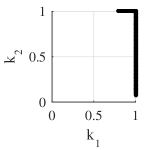
(a) $C_{1}^{s}=30\%,C_{2}^{s}=10\%$

(b) $C_{1}^{s}=50\%,C_{2}^{s}=10\%$

Figure 4: Pareto Frontier for $N_{1}=N_{2}=1$.

(a) $C_{1}^{s}=10\%,C_{2}^{s}=50\%$

(b) $C_{1}^{s}=20\%,C_{2}^{s}=50\%$

Figure 5: Pareto Frontier for $N_{1}=N_{2}=2$.

IV-C Bargaining solutions

The Pareto-frontier defines the set of partial pooling configurations from which one provider cannot improve its performance without degrading that of the other. That is, one cannot find a configuration that will be better for both providers simultaneously. Bargaining theory provides a framework for choosing one configuration from the set of Pareto-optimal ones [11]. While an extensive treatment of bargaining solutions is beyond the scope of the present paper, we now use one popular solution concept from the theory, namely, the Kalai-Smorodinsky bargaining solution (KSBS) [9], to capture the agreement point between the providers.

Definition 1.

A partial sharing configuration $(x_{1}^{*},x_{2}^{*})$ is a Kalai-Smorodinsky bargaining solution (KSBS), if $(x_{1}^{*},x_{2}^{*})$ is on the Pareto-frontier and satisfies

$$\frac{B_{1}(0,0)-B_{1}(x_{1}^{*},x_{2}^{*})}{B_{2}(0,0)-B_{2}(x_{1}^{*},x_{2}^{*})} ~{}=\frac{B_{1}(0,0)-\min\limits_{y\in[0,1]^{2}}B_{1}(y_{1},y_{2})}{B_{2}(0,0)-\min\limits_{y\in[0,1]^{2}}B_{2}(y_{1},y_{2})}.$$

The KSBS is such that the ratio of relative utilities of the providers is equal to the ratio of their maximal relative utilities. It can be shown (using arguments similar to those in [12]) that for $N_{1}=N_{2}=1$ and for the stationary waiting probability metric, the KSBS is uniquely defined. Table II illustrates the KSBS computed for various system parameters when $N_{1}=N_{2}=1.$ We see that when the providers are close to symmetric in their arrival rates (or equivalently, their standalone waiting probabilities), the KSBS corresponds to full pooling. On the other hand, when one provider is much more congested than the other, the KSBS does not correspond to complete pooling; only the more congested provider is required to always place its server into the common pool. Note that the KSBS affords a considerable improvement in performance for both providers.

TABLE II: Comparison of waiting probabilities (in %) for the case $N_{1}=N_{2}=1,$ respectively and $\nu_{1}=\nu_{2}=1$.

Standalone		Full Sharing	KSBS
$C_{1}^{s}$	$C_{2}^{s}$	$C_{1}=C_{2}=C$	$k_{1}^{*}$	$k_{2}^{*}$	$C_{1}(k_{1}^{*},k_{2}^{*})$	$C_{2}(k_{1}^{*},k_{2}^{*})$
10	10	1.82	1	1	1.82	1.82
10	30	6.65	0.69	1	5.54	14.54
10	50	13.85	0.37	1	8.26	37.30

V Discussions

In this section, we cover the special (and easier) single-server setting, where the service capacities of both providers can be merged into a single server. We also review the related literature, and outline potential directions for future work.

V-A Single server setting

First, we consider the special case where the service capacity of both providers can be combined into a single server. Moreover, the service capacity of this merged server is arbitrarily (and dynamically) divisible between the two providers. For this case, we define a balanced fairness (BF) based partial pooling mechanism between the providers, which includes both no pooling and complete pooling as special cases. For this mechanism, we show that complete pooling is the only Pareto-optimal configuration. Of course, given the equivalence between $\mathsf{c.o.c.}$ replication and single-server balanced-fair scheduling, and our conclusions from Section III, this is not surprising.

Consider two service providers $P_{1}$ and $P_{2}$ with servers operating at the rate (a.k.a. speed) $\mu_{1}$ and $\mu_{2}$ respectively. Recall that in this section, we consider the ‘single server’ setting, where it is possible to pool the capacity of the two servers into a single server with rate $\mu_{1}+\mu_{2}.$ Jobs of $P_{i}$ arrive according to a Poisson process of rate $\lambda_{i}$, and the service requirements (a.k.a. sizes) of jobs are i.i.d. and exponentially distributed with mean $1/\nu_{i}<\infty.$ Let $\rho_{i}:=\lambda_{i}/\nu_{i}$ denote the traffic load corresponding to $P_{i}.$ For stability, we assume that $\rho_{i}<\mu_{i}$ for $i=1,2.$

Jobs corresponding to each provider wait in separate queues, and are served in a FCFS fashion. The service rate for each queue is determined by a BF-based partial pooling mechanism, parametrized by $(k_{1},k_{2}).$ Here, $k_{i}\in[0,\mu_{i}]$ is a measure of the extent to which $P_{i}$ is willing to share its service capacity with $P_{-i}.$ Specifically, let $n_{i}$ denote the number of unfinished jobs of $S_{i}$ in the system. Given the system state $(n_{1},n_{2}),$ the BF-based partial pooling mechanism awards a service rate $r_{i}$ to Provider $i,$ such that $(r_{1},r_{2})$ is the balanced fair allocation over the rate region $\mathcal{R}(k_{1},k_{2})$ defined as follows:

$$\mathcal{R}(k_{1},k_{2})=\{(r_{1},r_{2})\in\, \mathbb{R}_{+}^{2}:\ r_{1}\leq\mu_{1}+k_{2},\;r_{2}\leq\mu_{2}+k_{1},\;$$

$$\quad r_{1}+r_{2}\leq\mu_{1}+\mu_{2}\}.$$

The shape of above rate region is similar to the rate region in Figure 2 with $N_{i}$ replace by $\mu_{i}$.

Theorem 4.

In the single server setting, under the BF-based partial pooling mechanism, the full sharing configuration (i.e., $k_{1}=\mu_{1},k_{2}=\mu_{2}$) is the only Pareto-optimal configuration, for the stationary waiting probability metric as well as the stationary mean response time metric.

Theorem 4 implies that the resource pooling problem is easy in the single server setting—complete pooling with balanced fair resource allocation is the solution.

V-B Related work

Complete resource pooling between independent service systems has been studied from a cooperative game theory standpoint; see, for example, [7, 1, 10]. The goal of this literature is to analyze stable mechanisms for sharing the surplus (and costs) of the grand coalition among the various agents. Single server as well as multi-server settings have been considered, for queueing as well as loss systems; see [10] for a comprehensive survey of this literature. A complementary view of resource sharing comes from an optimization standpoint. Here the organization is interested in optimally provisioning (potentially heterogenous) resources and/or sharing its service resources between various activities; see, for example, [3, 15, 8].

In contrast, our approach in this work is to analyze resource sharing between strategic service providers having non-transferable utility. In other words, no side-payments are allowed between the service providers. Instead, providers would (partially or completely) pool their resources with one another only if their service quality improves in the process. Our goal is thus to devise mechanisms that guarantee mutually beneficial sharing configurations. The only prior work we are aware of that takes this view is [12], which considers loss systems. In contrast, the present paper considers service systems where jobs can be queued. As it turns out, the appropriate sharing mechanisms are very different between these two settings.

V-C Naive partial sharing

In this paper, we analyzed partial sharing for systems with full redundancy, i.e., copies are sent to all the servers. An alternative system that would have been a natural generalization of the partial sharing with blocking analyzed in [12] would be to have three separate queues—one each for the two dedicated servers and one for the shared servers—and send an incoming job with priority to the dedicated servers. Repacking could have been used to dynamically exchange servers between the pools in order to ensure that the stability region is the same as in this paper. Compared to the redundancy system, the naive system presents an inconvenience in that it is not easy to show whether or not it admits a product-form. For the computation of the waiting probability, this is a major disadvantage. One could in theory use sample-path techniques employed in [12] to characterize the Pareto-frontier, but these become much more involved for the system in this paper and we are not sure that they are even true. This is part of our ongoing work.

V-D Future work

An immediate avenue for future work is of course to prove Conjecture 1 and completely analyse the Pareto-frontier under $\mathsf{c.o.s.}$ replication; this is currently being pursued. It would also be interesting to generalize our models to $n>2$ service providers, and to devise suitable partial sharing mechanisms that guarantee the existence of mutually beneficial sharing configurations.

More broadly, the present bargaining-centric view of resource pooling (with non-transferable utilities between agents) can be explored in other contexts; for example, sharing of cache memory between content distribution systems, sharing of energy storage in smart power grids, and spectrum sharing between cellular service providers or between secondary users in cognitive radio networks.

Appendix A Proof of Lemma  1

We derive the expression for mean response time for a partially pooled system with sharing configuration $(k_{1},k_{2})$ with c.o.c. replication using the equivalence of its steady state system occupancy vector with that of balanced fair scheduling as mentioned in Section III. Theorem 4 in [13] provides following general expression mean response time under balanced fair scheduling and thus also for for a partially pooled system with sharing configuration $(k_{1},k_{2})$ with c.o.c. replication.

$$D_{i}(k_{1},k_{2})=\frac{\nu_{i}\frac{\partial G(k_{1},k_{2})}{\partial\rho_{i}}}{G(k_{1},k_{2})}.$$ (1)

Given $G(k_{1},k_{2})$, by differentiating it wrt $\rho_{i}$ and substituting it in Equation 1, we get the expression for mean response time.

$G(k_{1},k_{2})$ can be calculated using following equations stated in [13]: Let $G_{\{\phi\}}=1$ and for $\mathcal{A}\in\{\{1\},\{2\},\{1,2\}\}$, $G_{\mathcal{A}}$ is defined as:

$$G_{\mathcal{A}}=\frac{\sum_{i\in A}\rho_{i}G_{A-i}}{\mu(\mathcal{A})-\sum_{j\in\mathcal{A}}\rho_{j}}.$$

$\mu(\mathcal{A})$ is the maximum service rate for the set of providers $\mathcal{A}$ in the balanced fair rate allocation as shown in Figure 2. Hence,

$$G_{\{1\}}=\frac{\rho_{1}}{N_{1}+k_{2}-\rho_{1}},G_{\{2\}}=\frac{\rho_{2}}{N_{2}+k_{1}-\rho_{2}},$$

$$G_{\{1,2\}}=\frac{\rho_{1}G_{\{2\}}+\rho_{2}G_{\{1\}}}{N_{1}+N_{2}-\rho_{1}-\rho_{2}}=\rho_{1}\rho_{2}\frac{\frac{1}{N_{1}-\rho_{1}}+{\frac{1}{N_{2}-\rho_{2}}}}{N_{1}+N_{2}-\rho_{1}-\rho_{2}}.$$

$G(k_{1},k_{2})=G_{\{\phi\}}+G_{\{1\}}+G_{\{2\}}+G_{\{1,2\}}$. By substituting the values $G_{\{\phi\}},G_{\{1\}}G_{\{2\}}$, $G_{\{1,2\}}$ and rearranging some terms, we get

$$G(k_{1},k_{2})=\frac{1}{1-\frac{\rho_{1}+\rho_{2}}{N_{1}+N_{2}}}\bigg{(}\frac{1-\frac{\rho_{1}}{N_{1}+k_{2}}}{1-\frac{\rho_{1}}{N_{1}+N_{2}}}+\frac{1-\frac{\rho_{2}}{N_{2}+k_{1}}}{1-\frac{\rho_{2}}{N_{1}+N_{2}}}-1\bigg{)}.$$

Appendix B Proof of Lemma  2

1) The mean response time of the overall system $D(k_{1},k_{2})$ is given by: $D(k_{1},k_{2})=\frac{\lambda_{1}}{\lambda_{1}+\lambda_{2}}D_{1}(k_{1},k_{2})+\frac{\lambda_{2}}{\lambda_{1}+\lambda_{2}}D_{2}(k_{1},k_{2})$. On simplification we get,

$$D(k_{1},k_{2})=\frac{\rho_{1}+\rho_{2}}{N_{1}+N_{2}-\rho_{1}-\rho_{2})}+\frac{L_{1}(k_{1},k_{2})+L_{2}(k_{1},k_{2})}{H(k_{1},k_{2})}$$

where,
$H(k_{1},k_{2})=\bigg{(}\frac{1-\frac{\rho_{1}}{N_{1}+N_{2}}}{1-\frac{\rho_{1}}{N_{1}+k_{2}}}+\frac{1-\frac{\rho_{2}}{N_{1}+N_{2}}}{1-\frac{\rho_{2}}{N_{2}+k_{1}}}-1\bigg{)}$ and $L_{i}(k_{1},k_{2})=\frac{\frac{p_{i}}{N_{i}+k_{-i}}-\frac{p_{i}}{N_{1}+N_{2}}}{\big{(}1-\frac{p_{i}}{N_{i}+k_{-i}}\big{)}^{2}}.$ Now we show that the overall mean response time decrease with $k_{i}$.

$$\frac{\partial{D}}{\partial k_{2}}= \frac{-\rho_{1}}{H^{2}(N_{i}+k_{-i})^{2}}\Bigg{[}\frac{\big{(}1-\frac{\rho_{1}}{N_{1}+N_{2}}\big{)}^{2}}{\big{(}1-\frac{p_{1}}{N_{1}+k_{2}}\big{)}^{4}}$$

$$+\frac{L_{2}\big{(}1-\frac{\rho_{2}}{N_{2}+k_{1}}\big{)}}{\big{(}1-\frac{p_{1}}{N_{1}+k_{2}}\big{)}^{2}}\Bigg{(}2\frac{\big{(}1-\frac{\rho_{1}}{N_{1}+N_{2}}\big{)}}{\big{(}1-\frac{p_{1}}{N_{1}+k_{2}}\big{)}}-1\Bigg{)}+L_{2}\Bigg{]}<0.$$

$\frac{\partial{D}_{1}}{\partial k_{2}}=\frac{\lambda_{1}+\lambda_{2}}{\lambda_{1}}\Big{(}\frac{\partial{D}(k_{1},k_{2})}{\partial k_{2}}-\frac{\lambda_{1}}{\lambda_{1}+\lambda_{2}}\frac{\partial{D}_{1}(k_{1},k_{2})}{\partial k_{2}}\Big{)}<0.$

2) If $k_{-i}=N_{-i}$,then is easy to note that $D_{i}(k_{1},k_{2})$ depends on $k_{i}$ only through $H(k_{1},k_{2})$. Since $H(k_{1},k_{2})$ is strictly decreasing function of $k_{i}$, $D_{i}(k_{1},k_{2})$ increases with $k_{i}$.

3) If $k_{-i}=N_{-i}$, $D_{i}(k_{1},k_{2})=\frac{\nu_{i}}{N_{1}+N_{2}-\rho_{1}-\rho_{2}}$, does not depend on $k_{i}$.

Appendix C Performance Characterization with $\mathsf{c.o.s.}$

C-A Assignment Rates

We provide a detailed approach for computing the steady-state distribution and hence the expressions for $C_{i}(k_{1},k_{2})$ and $D_{i}(k_{1},k_{2})$. We introduce the following notations:

$$\mathcal{M}_{1}= \{1,\cdots N_{1}-k_{1}\}\text{, dedicated servers of }P_{1},$$

$$\mathcal{M}_{2}= \{N_{1}+k_{2}+1,\cdots N_{1}+N_{2}\}\text{, dedicated servers of }P_{2},$$

$$\mathcal{M}_{3}= \{N_{1}-k_{1}+1,\cdots N_{1}+k_{2}\}\text{, shared servers.}$$

For a given subset of servers $m=\{m_{1},\cdots,m_{j},m_{k}\}$, define $x_{i}(m)=$ number of servers from the set $\mathcal{M}_{i}$ in $m$ and $x(m)=(x_{1}(m),x_{2}(m),x_{3}(m))$. Also define $\bar{x}(m)=(\bar{x}_{1}(m),\bar{x}_{2}(m),\bar{x}_{3}(m))$ where $\bar{x}_{i}(m)=|\mathcal{M}_{i}|-x_{i}(m)$ and $e_{i}$ be the unit vector in the direction $i$.

All servers in $\mathcal{M}_{i}$ are identical, hence $\lambda_{m_{j}}\{m\}$ is same for all $m_{j}\in\mathcal{M}_{i}$ for $i=1,2,3.$ Using the assignment rate condition it can also be shown that $\lambda_{m_{j}}\{m\}=\lambda_{m_{j}}\{m^{\prime}\}$ if $x(m)=x(m^{\prime})$. Hence, we can define $r_{i}(x(m))=\lambda_{m_{j}}\{m\}$ for $m_{j}\in\mathcal{M}_{i}$ and $m\in\mathcal{M}$. Since the vector $x$ takes values from a finite set $\mathcal{X}(\in\mathds{Z}^{3}$), calculating $r_{i}(x)$ for all values in $\mathcal{X}$ gives all the assignment rate probabilities $\lambda_{m_{j}}\{m\}$.

Recall that $\lambda(m)$ is the aggregate arrival rate corresponding to jobs which cannot be served by any server in the set $\mathcal{M}\setminus m$. Define $\bar{\lambda}(m)=\lambda_{1}+\lambda_{2}-\mathcal{M}\setminus m$, the aggregate arrival rate corresponding to jobs which can be served by the servers in $\mathcal{M}\setminus m$, note that $\bar{\lambda}(m)=\bar{\lambda}(m^{\prime})$ if $x(m)=x(m^{\prime})$. Hence $r(x(m))=\bar{\lambda}(m)$. Using this and the assignment rate condition stated in Section IV, we obtain the following set of equations between $r_{i}(x)$, which can be solved to get $r_{i}(x)$ for all $x\in\mathcal{X}$ and $i=1,2,3$.

$$\bar{x}_{1}r_{1}(x)+\bar{x}_{2}r_{2}(x)+\bar{x}_{3}r_{3}(x)=r(x).$$

For $x\in\mathcal{X}\text{ such that }x_{1}<N_{1}-k_{1}\text{ and }x_{3}<k_{1}+k_{2},$

$$r_{1}(x)r_{3}(x+e_{1})=r_{1}(x+e_{3})r_{3}(x).$$

For $x\in\mathcal{X}\text{ such that }x_{2}<N_{2}-k_{2}\text{ and }x_{3}<k_{1}+k_{2},$

$$r_{2}(x)r_{3}(x+e_{2})=r_{2}(x+e_{3})r_{3}(x).$$

$$r_{i}((N_{1}-k_{1},N_{2}-k_{2},k_{1}+k_{2})-e_{i})=\begin{cases}\lambda_{1}\text{ if }i=1,\\ \lambda_{2}\text{ if }i=2,\\ \lambda_{1}+\lambda_{2}\text{ if }i=3.\end{cases}$$

$$r_{i}(x)=0\text{ if }x_{i}=|\mathcal{M}_{i}|.$$

$$\text{Recall that, }\Pi_{\lambda}(\{m_{1},\cdots,m_{i}\})=\prod_{j=1}^{i}\lambda_{m_{j}}{(\{m_{1},\cdots,,m_{j-1}\})}.$$

Again due to the assignment rate condition, $\Pi_{\lambda}(m)=\Pi_{\lambda}(m^{\prime})$ if $x(m)=x(m^{\prime})$, hence we define $\Pi(x(m))=\Pi_{\lambda}(m)$.

C-B The Waiting Probability

For a state $s=(n_{i},m_{i},\cdots,n_{2},m_{2},n_{1},m_{1})$, $m(s)$ is the set of busy servers., i.e, $m(s)=\{m_{1},m_{2}\cdots,m_{i}\}$. then the waiting probability $C_{i}(k_{1},k_{2})$ is follows:

$$C_{1}(k_{1},k_{2})=\sum_{s:x_{1}(m(s))+x_{3}(m(s))=N_{1}+k_{2}.}\pi(s).$$

Let us define $\pi_{\{\mathcal{A}\}}$ as the probability that an arriving job of the provider $\mathcal{A}$ has to wait ($\mathcal{A}\in\{\{\phi\},\{1\},\{2\},\{1,2\}\}$). Equivalently, $\pi_{\{\mathcal{A}\}}$ is the sum of stationary probabilities of those states in which all servers which can serve jobs from providers $\mathcal{A}$ are busy. Then the waiting probabilities for Provider $P_{i}$ can be expressed as,

$$C_{i}(k_{1},k_{2})=\pi_{\{i\}}+\pi_{\{1,2\}},$$

where, $\pi_{\{1\}}=\sum_{s:x_{1}(m(s))+x_{3}(m(s))=N_{1}+k_{2},x_{2}(m(s)<N_{2}-k_{2}}\pi(s).$ After obtaining the assignment probabilities and then using the expression for $\pi(s)$ from Theorem 2, we get $\pi_{\{1\}}=\sum\limits_{x_{2}=0}^{N_{2}-k_{2}-1}\frac{\Pi(N_{1}-k_{1},y,k_{1}+k_{2})\pi(0)}{(N_{1}+k_{2}+x_{2})!}{N_{2}-k_{2}\choose y}\Bigg{(}\sum_{w=0}^{x_{2}}{x_{2}\choose w}w!(N_{1}+k_{2})(N_{1}+k_{2}+x_{2}-w-1)!\bigg{(}\Pi_{v=0}^{w}\frac{(N_{1}+k_{2}+x_{2}-w+v)}{(N_{1}+k_{2}+x_{2}-w+v-\lambda_{1})}\bigg{)}\Bigg{)}.$ Similarly, we can write the expression for $\pi_{\{2\}}$ using symmetry, also $\pi_{\{1,2\}}=\sum_{s:x_{1}(m(s))+x_{2}(m(s))+x_{3}(m(s))=N_{1}+N_{2}}\pi(s)$,

$\pi_{\{1,2\}}=\frac{\Pi(N_{1}-k_{1},N_{2}-k_{2},k_{1}+k_{2})\pi(0)}{(N_{1}+N_{2}-1)!(N_{1}+N_{2}-\lambda_{1}-\lambda_{2})}\Bigg{(}\sum_{w=0}^{N_{2}-k_{2}}{N_{2}-k_{2}\choose w}w!\\ (N_{1}+k_{2})(N_{1}+N_{2}-w-1)!\bigg{(}\Pi_{v=0}^{w-1}\frac{(N_{1}+N_{2}-w+v)}{(N_{1}+N_{2}-w+v-\lambda_{1})}\bigg{)}\Bigg{)}$.

Similarly the expression for mean response time can be computed, which is omitted due to lack of space. As one can see these expressions though easy to compute numerically are not very amenable to analysis.

Appendix D Proof of Theorem  3

The proof of Theorem 3 is structured as follows: first we show that $C_{i}(k_{1},k_{2})$ satisfies a set of 3 conditions in Lemma 3. Then we show that if those conditions are satisfied then Pareto region lies on the boundary, i.e. at least one of the $k_{i}=N_{i}$. After showing that the Pareto-frontier lies on the boundary, the explicit structure of the Pareto-frontier described in Theorem 3 is direct consequence of the monotonicity properties as shown in [12]. The proof is omitted due to lack of space.

Lemma 3.

For $\mathsf{c.o.s.}$ replication and $N_{1}=1$ and $N_{2}=1$

1. $C_{i}(k_{1},k_{2})$ is a strictly decreasing function of $k_{-i},$

2. $C_{i}(k_{1},k_{2})$ is a strictly increasing function of $k_{i},$

3. $\frac{\partial C_{1}}{\partial k_{2}}\frac{\partial C_{2}}{\partial k_{1}}>\frac{\partial C_{1}}{\partial k_{1}}\frac{\partial C_{2}}{\partial k_{2}}.$

Proof.

As defined in Section IV, for any $k_{1}\in[0,1]\text{ and }k_{2}\in[0,1],$ the waiting probability is given by:

$$C_{i}(k_{1},k_{2})=(1-k_{1})(1-k_{2})C_{i}(0,0)+(k_{1})(1-k_{2})C_{i}(1,0)$$

$$+(1-k_{1})k_{2}C_{i}(0,1)+k_{1}k_{2}C_{i}(1,1),$$

where $C_{i}(0,0),C_{i}(1,0),C_{i}(0,1)$ and $C_{i}(0,1)$ can be explicitly computed using the results in Appendix C. For the sake of tidiness, we use the notation $C_{i}$ instead of $C_{i}(k_{1},k_{2})$ for the rest of the proof. For $i=1$,

$$\frac{\partial C_{1}}{\partial k_{1}}= (1-k_{2})\big{[}C_{1}(1,0)-C_{1}(0,0)\big{]}+k_{2}[C_{1}(1,1)-C_{1}(0,1)\big{]}$$

$$= \frac{(1-k_{2})}{\Omega_{1}}(2-\lambda_{1}+\lambda_{2}-\lambda_{1}\lambda_{2}-\lambda_{1}^{2})\lambda_{2}^{2}$$

$$+\frac{k_{2}}{\Omega_{2}}(2-\lambda_{1}-\lambda_{2})\lambda_{2}(\lambda_{1}+\lambda_{2})^{2}>0.$$

$$\frac{\partial C_{1}}{\partial k_{2}}= (1-k_{1})\big{[}C_{1}(0,1)-C_{1}(0,0)\big{]}+k_{1}[C_{1}(1,1)-C_{1}(1,0)\big{]}$$

$$= \frac{(1-k_{1})}{\Omega_{2}}\lambda_{1}(1-\lambda_{2})[\lambda_{1}(\lambda_{2}-4)+\lambda_{2}(\lambda_{2}-2)]$$

$$+\frac{k_{1}}{\Omega_{1}}(\lambda_{1}\lambda_{2}+\lambda_{2}^{2}+2\lambda_{1}-4)(\lambda_{1}+\lambda_{2})^{2}<0,$$

where
$\Omega_{1}=(\lambda_{1}+\lambda_{2}+\lambda_{2}^{2})(1-\lambda_{1})+\lambda_{1}(1-\lambda_{1}\lambda_{2})+3\lambda_{2}+\lambda_{2}^{2}>0,$
$\Omega_{2}=(\lambda_{1}+\lambda_{2}+\lambda_{1}^{2})(1-\lambda_{2})+\lambda_{2}(1-\lambda_{1}\lambda_{2})+3\lambda_{1}+\lambda_{1}^{2}>0.$ Similarly due to symmetry, it can be shown that $\frac{\partial C_{2}}{\partial k_{1}}<0$ and $\frac{\partial C_{2}}{\partial k_{2}}>0$. Hence, $C_{i}(k_{1},k_{2})$ is a strictly decreasing function of $k_{-i},$ and $C_{i}(k_{1},k_{2})$ is a strictly increasing function of $k_{i}.$

$$\frac{\partial C_{1}}{\partial k_{2}}\frac{\partial C_{2}}{\partial k_{1}}-\frac{\partial C_{1}}{\partial k_{1}}\frac{\partial C_{2}}{\partial k_{2}}=\;\alpha k_{1}+\beta k_{2}+\gamma,$$

where,

$$\alpha= \big{[}C_{1}(1,0)-C_{1}(0,0)\big{]}\big{[}C_{2}(0,1)-C_{2}(1,1)\big{]}-$$

$$\big{[}C_{1}(1,1)-C_{1}(0,1)\big{]}\big{[}C_{2}(0,0)-C_{2}(1,0)\big{]}$$

$$= \frac{2(1-\lambda_{1})(2-\lambda_{1}-\lambda_{2})(2+\lambda_{1}-\lambda_{2}+\lambda_{1}^{2}+\lambda_{1}\lambda_{2})}{(2+\lambda_{1}+\lambda_{2})\Omega_{1}\Omega_{2}}>0,$$

$$\beta= \big{[}C_{1}(1,0)-C_{1}(1,1)\big{]}\big{[}C_{2}(0,1)-C_{2}(0,0)\big{]}-$$

$$\big{[}C_{1}(0,0)-C_{1}(0,1)\big{]}\big{[}C_{2}(1,1)-C_{2}(1,0)\big{]}$$

$$= \frac{2(1-\lambda_{2})(2-\lambda_{1}-\lambda_{2})(2+\lambda_{2}-\lambda_{1}+\lambda_{2}^{2}+\lambda_{1}\lambda_{2})}{(2+\lambda_{1}+\lambda_{2})\Omega_{1}\Omega_{2}}>0,$$

$$\gamma= \big{[}C_{1}(0,0)-C_{1}(0,1)\big{]}\big{[}C_{2}(0,0)-C_{2}(1,0)\big{]}-$$

$$\big{[}C_{1}(1,0)-C_{1}(0,0)\big{]}\big{[}C_{2}(0,1)-C_{2}(0,0)\big{]}$$

$$= \frac{4\lambda_{1}\lambda_{2}(1-\lambda_{1})(1-\lambda_{2})(2-\lambda_{1}-\lambda_{2})}{\Omega_{1}\Omega_{2}}>0.$$

Hence we have, $\frac{\partial C_{1}}{\partial k_{2}}\frac{\partial C_{2}}{\partial k_{1}}-\frac{\partial C_{1}}{\partial k_{1}}\frac{\partial C_{2}}{\partial k_{2}}>0.$ ∎

Now given that the Lemma 3 holds, we show that the Pareto Frontier lies on the boundary as follows: we show that for any $(k_{1},k_{2})$ where $k_{i}\in[0,N_{i})$, there exists a $\theta$ such that $\nabla C_{i}(k_{1},k_{2})\cdot(1,\theta)<0\text{ for }i=1,2.$ $C_{1}(k_{1},k_{2})\cdot(1,\theta)>0$ and $C_{2}(k_{1},k_{2})\cdot(1,\theta)>0$ are equivalent, respectively, to

$$\theta>-\frac{\frac{\partial C_{1}}{\partial k_{1}}}{\frac{\partial C_{1}}{\partial k_{2}}},\quad\theta<-\frac{\frac{\partial C_{2}}{\partial k_{1}}}{\frac{\partial C_{2}}{\partial k_{2}}}.$$

Therefore if Statement 3 of Lemma 3 holds, there exists a direction $\theta$ along which both providers will have lower values of $C_{i}(k_{1},k_{2})$ and hence any such configuration cannot be Pareto-optimal.

References

- [1] S. Anily and M. Haviv, “Cooperation in service systems,” Operations Research, vol. 58, no. 3, pp. 660–673, May-June 2010.
- [2] U. Ayesta, T. Bodas, and I. M. Verloop, “On a unifying product form framework for redundancy models,” Performance Evaluation, vol. 127, pp. 93–119, 2018.
- [3] S. Benjaafar, “Performance bounds for the effectiveness of pooling in multi-processing systems,” European Journal of Operational Research, vol. 87, no. 2, pp. 375–388, 1995.
- [4] T. Bonald, C. Comte, and F. Mathieu, “Performance of balanced fairness in resource pools: A recursive approach,” Proceedings of the ACM on Measurement and Analysis of Computing Systems, vol. 1, no. 2, p. 41, 2017.
- [5] T. Bonald and A. Proutiere, “Insensitive bandwidth sharing in data networks,” Queueing systems, vol. 44, no. 1, pp. 69–100, 2003.
- [6] K. Gardner, M. Harchol-Balter, A. Scheller-Wolf, M. Velednitsky, and S. Zbarsky, “Redundancy-d: The power of choices for redundancy,” Operations Research, vol. 65, no. 4, pp. 1078–1094, 2017.
- [7] P. González and C. Herrero, “Optimal sharing of surgical costs in the presence of queues,” Mathematical Methods of Operations Research, vol. 59, no. 3, pp. 435–446, 2004.
- [8] S. M. Iravani, B. Kolfal, and M. P. Van Oyen, “Call-center labor cross-training: It’s a small world after all,” Management Science, vol. 53, no. 7, pp. 1102–1112, 2007.
- [9] E. Kalai and M. Smorodinsky, “Other solutions to nash’s bargaining problem,” Econometrica, vol. 43, no. 3, pp. 513–518, 1975.
- [10] F. Karsten, M. Slikker, and G.-J. Van Houtum, “Resource pooling and cost allocation among independent service providers,” Operations Research, vol. 63, no. 2, pp. 476–488, 2015.
- [11] R. B. Myerson, Game theory. Harvard University Press, 2013.
- [12] A. Nandigam, S. Jog, D. Manjunath, J. Nair, and B. Prabhu, “Sharing within limits: Partial resource pooling in loss systems,” arXiv preprint arXiv:1808.06175, 2018.
- [13] V. Shah and G. de Veciana, “Performance evaluation and asymptotics for content delivery networks,” in IEEE INFOCOM, 2014.
- [14] J. Visschers, I. Adan, and G. Weiss, “A product form solution to a system with multi-type jobs and multi-type servers,” Queueing Syst. Theory Appl., vol. 70, no. 3, pp. 269–298, 2012.
- [15] R. B. Wallace and W. Whitt, “A staffing algorithm for call centers with skill-based routing,” Manufacturing & Service Operations Management, vol. 7, no. 4, pp. 276–294, 2005.