Landau theory for smectic-A – hexatic-B coexistence in smectic films

Abstract

We explain theoretically peculiarities of the smectic $A$ – hexatic $B$ equilibrium phase coexistence in a finite temperature range recently observed experimentally in free standing smectic films [I.A.Zaluzhnyy et al., Physical Review E, 98, 052703 (2018)]. We quantitatively describe this unexpected phenomenon within Landau phase transitions theory assuming that the film state is close to a tricritical point. We found that the surface hexatic order leads to diminishing the phase coexistence range as the film thickness decreases shrinking it at some minimal film thickness $L_{c}$, of the order of the hexatic correlation length. We established universal laws for the temperature width of the phase coexistence in terms of the reduced variables. Our theory is in agreement with the existing experimental data.

Keywords free standing smectic films, hexatic order parameter, Landau theory of phase transitions

I Introduction

Free standing smectic films are unique layered systems, solid-like in one direction (normal to the layers) and fluid-like in two lateral directions. Unlike other films, smectic films are living in three-dimensional world without any parasitic influence from a substrate. It is not surprising that this topic is the subject of many experimental and theoretical works (see, e.g., the comprehensive review JO03 and the monograph PP06 ). Our motivation to add one more article to the investigation field is related to new results, concerning the phase coexistence in smectic films, we obtained. Our main concern is related to finite-size effects.

In our study we developed the quantitative theory explaining the finite temperature interval for the equilibrium coexistence of the smectic $A$ and the hexatic $B$ phases in the smectic films. Common wisdom claims that the equilibrium phase coexistence at the first order phase transition takes place at the transition temperature solely. A finite range for the phase coexistence can be achieved for binary mixtures, or (in the case of single-component materials) in confined geometry, where neither of the coexistent states can provide the required equilibrium density. However, we consider one-component material and in apparently unconfined free standing film geometry. The point is that any smectic liquid crystal is strongly anisotropic and solid-like along the normal to smectic layers. Due to this anisotropy, smectic stress tensor component orthogonal to the smectic layers, is not determined uniquely by the external pressure, an essential contribution comes from the solid-like elasticity of smectic layers (see more details in Refs. JO03 ; PP06 ). As a result, smectic films behave similarly to a closed volume system undergoing the first order phase transition under condition that the number of the smectic layers is fixed (i.e., unchanged on a time scale needed to get the equilibrium phase coexistence). The standard experimental technique for the free standing smectic film preparation, indeed, provides the uniform film thickness Stoebe94 ; Dolganov95 ; Picano01 ; Ostrovskii03 ; ZK18 . In turn, local changes in the film thickness are possible only under overheating of the free standing smectic film above the bulk temperature of melting of smectic phase or under local (nonuniform) heating of the films, see Refs. Stoebe94 ; Dolganov95 ; Picano01 ; Stoebe95 ; Demikhov95 ; Huang97 ; Ostrovskii04 ; Stannarius08 ; PO15 ; PO17 . These non-equilibrium phenomena are beyond our consideration.

In the majority of the materials, exhibiting $SmA$ – $HexB$ phase transition, the transition turns out to be weak first order phase transitions, see Refs. JV95 ; HK97 ; RD05 ; MP13 ; ZK18 . A tempting explanation of the fact based on closeness to a critical point, is excluded since the states have different symmetries ($SmA$ possesses isotropic liquid-like smectic layers, and $HexB$ possesses orientation hexagonal symmetry order). We suggest another possibility to explain the experimental data, that the system is close to a tricritical point. This assumption is supported also by the measured critical exponents (for the specific heat and for the order parameter) that are close to those for the tricritical point JV95 ; HK97 ; RD05 ; MP13 . It is worth to note that the liquid-crystalline materials exhibiting the $SmA$ – $HexB$ phase transition demonstrate apparently universal behavior. The phase diagrams of such materials are remarkably similar even though the molecules of the materials are appreciably different (see, for example, JV96 ; ZK17 ). Thus our results are universal and can be applied to all the materials.

We exploit the phenomenological Landau phase transitions theory. As it is known, the mean field Landau theory works well near the tricritical point (up to logarithmic corrections), see, e.g., LL80 ; ST87 ; AN91 . Our calculations are mainly analytical, giving the frame for observable effects. They are expressed as universal laws in terms of reduced variables. To find solutions of the non-linear equations within the whole temperature interval of the phase coexistence we use Wolfram Mathematica numerics. This allow us to illustrate dependencies for the width of the equilibrium phase coexistence on system parameters. We also compute numeric values of the dimensionless coefficients entering the derived analytically universal laws.

In the work ZK18 the coexistence of $SmA$ and $HexB$ phases were observed in a finite temperature interval (and qualitatively and semi-quantitatively, for thick films, rationalized theoretically). However, presented in the paper ZK18 the expression for the temperature interval of the equilibrium phase coexistence has been derived merely from the surface order induced renormalization of the bulk hexatic phase parameters (what is not a consistent procedure). In this work we present the consistent quantitative theory.

Our paper is organized as follows. In the next section II we formulate general thermodynamical conditions for the phase coexistence, in a form suitable for smectic liquid crystals, possessing the layer structure. In the subsection II.1 of this section II we discuss the phase coexistence in bulk in terms of the Landau theory. Specifically motivated by experimental observations ZK18 we study $SmA$ – $HexB$ transition in the free standing films. In the section III we explore and analyze the key point of our work, namely the surface effects. In the free standing smectic films exhibiting $SmA$ – $HexB$ phase transition, the surface hexatic order occurs at the temperature higher than the bulk transition temperature. This surface induced order in the vicinity of a tricritical point penetrates into the interior of the film, what essentially influences the phase transition even for the relatively thick films. In particular we demonstrate that the surface order provokes diminishing the phase coexistence range as the film thickness decreases. Eventually, it leads to shrinking the coexistence range at some minimal film thickness $L_{c}$. Thus we arrive at a special critical point, where the coexisting phases become indistinguishable. In the concluding section IV, we summarize our results, and also discuss some open questions and perspectives. We relegate some technical details of the analytic calculations into two appendices to the main text.

II General thermodynamic analysis of the phase coexistence

Here, we remind the general thermodynamical conditions of the phase coexistence LL80 ; HU87 . Two phase coexistence indicates that none of the coexisting phases (in our case $SmA$ and $HexB$) is able to support the optimal two-dimensional density of the film, and the compromise is achieved by means of two-phase equilibrium where two phases coexist. The coexistence signals about first order transition between the phases. However, ordering in the hexatic case is weak in the region of the phase coexistence. That enables one to use the Landau expansion in the order parameter to analyze the phenomenon. We consider the case where the number of the smectic layers in the film is fixed. The assumption holds if nucleation of dislocation loops (which are able to adjust the number of layers to the external stresses) is very infrequent and too slow in comparison to characteristic time scales relevant for the phase coexistence PP01 ; PP06 ; OP18 . Then the thickness $L$ of the film is determined as a minimum condition of an appropriate thermodynamic potential. Although the thicknesses of the $SmA$ and $HexB$ phases are slightly different (at a given temperature), due to the weakness of the hexatic ordering the difference is small and can be safely neglected.

We designate as $N_{H}$ and $N_{A}$ two-dimensional mass densities and designate as $F_{H}$ and $F_{A}$ two-dimensional free energy densities of the $HexB$ and of the $SmA$ phases, respectively. If areas that the phases occupy are $A_{H}$ and $A_{A}$, then the total free energy of the system can be written as

$${\cal F}=F_{A}(N_{A})A_{A}+F_{H}(N_{H})A_{H}$$

$$-\mu(N_{A}A_{A}+N_{H}A_{H}-{\cal N}),$$ (1)

where ${\cal N}$ is the total number of molecules in the film and $\mu$ is a Lagrangian multiplier fixing the number. Minimization of the energy (1) in terms of $N_{A}$ and $N_{H}$ leads to the conditions

$$\frac{\partial F_{A}}{\partial N_{A}}=\mu=\frac{\partial F_{H}}{\partial N_{H}}.$$ (2)

Thus the chemical potentials of the phases are equal if they coexist. This condition is analogous to famous Maxwell common tangent construction, see Refs. HU87 ; ST87 ; AN91 ; CL00 .

Note that $A_{H}=A-A_{A}$, where $A$ is the total area of the film. Therefore minimization of the expression (1) in terms of $A_{A}$ leads to the condition

$$\Omega_{A}=\Omega_{H},$$ (3)

where $\Omega$ is the grand thermodynamic potential per unit area:

$$\Omega(\mu)=F-N\frac{\partial F}{\partial N},\quad\mu=\frac{\partial F}{\partial N},$$

$$d\Omega=-Nd\mu-SdT.$$ (4)

Further we operate in terms of the grand thermodynamic potential having in mind that both, the chemical potentials and the temperatures of the coexisting phases should coincide.

We arrived at the following general picture of the phase transitions. At $T>T_{+}$ the smectic-A phase is realized. Then the chemical potential $\mu$ is determined by the condition $\partial\Omega_{A}/\partial\mu=-N$, where $N={\cal N}/A$ is the average two-dimensional density of molecules of the film. At $T<T_{-}$ the hexatic phase is realized. Then the chemical potential $\mu$ is determined by the condition $\partial\Omega_{H}/\partial\mu=-N$. At $T_{-}<T<T_{+}$ the phases coexist, then the chemical potential $\mu$ is determined by the condition (3). Thus, the chemical potential $\mu_{+}$ at $T=T_{+}$ is determined by the relation (3) and the condition $\partial\Omega_{A}/\partial\mu=-N$.

Below $T_{+}$, in the region of the phase coexistence, the density of the smectic-A phase $N_{A}=-\partial\Omega_{A}/\partial\mu$ does not coincide with $N$. We expect that it is larger than $N$: $N_{H}<N<N_{A}$. Having in mind narrowness of the coexistence region, we expand the density of the smectic-A phase in $\mu-\mu_{+}$, $T-T_{+}$ to obtain

$$N_{A}=N-\frac{\partial^{2}\Omega_{A}}{\partial\mu^{2}}(\mu-\mu_{+})-\frac{\partial^{2}\Omega_{A}}{\partial T\partial\mu}(T-T_{+}),$$ (5)

where the derivatives are taken at $T=T_{+}$, $\mu=\mu_{+}$.

II.1 Landau expansion

The hexatic order parameter $\psi$ (see its definition in CL00 ; GP93 and its symmetry derivation in GKL91 ) in the region of the phase coexistence is assumed to be small. Then one may expand the grand thermodynamic potential $\Omega$ in $\psi$ to obtain $\Omega=\Omega_{0}+\Phi$ where $\Phi$ is the Landau functional. In the context of the bulk consideration (neglecting surface effects) the first terms of its expansion in $\psi$ are

$$\Phi=L\left(a\,|\psi|^{2}\,-\,\lambda\,|\psi|^{4}/6\,+\,\zeta|\psi|^{6}/90\right),$$ (6)

where $L$ is the thickness of the film and the coefficients $a,\lambda,\zeta$ are functions of $T,\mu$.

We expanded the grand thermodynamic potential $\Omega$ up to the sixth order in $\psi$ having in mind that both coefficients, $a$ and $\lambda$, are anomalously small. By other words, we are in the tricritical regime (near a tricritical point in the phase diagram). It is well known LL80 ; ST87 ; AN91 that in the tricritical regime fluctuations of the order parameter are relatively weak: they produce only logarithmic corrections to observable quantities. Therefore our problem can be examined in the mean field approximation.

To find equilibrium values of the order parameter $\psi$, one should minimize the Landau functional (6). The smectic-A phase corresponds to zero value of the order parameter $\psi$. The minimum of $\Phi$ at $\psi=0$ is realized if $a>0$, the condition is implied below. The hexatic phase corresponds to a non-zero order parameter, that can be found as a result of the minimization:

$$|\psi_{m}|^{2}=\frac{5\lambda}{\zeta}\left(1+\sqrt{1-\frac{6a\zeta}{5\lambda^{2}}}\right).$$ (7)

This minimum of the Landau functional exists if $6a\zeta<5\lambda^{2}$.

In the mean field approximation the Landau functional $\Phi$ is equal to zero for the smectic-A phase. Therefore $\Omega_{A}=\Omega_{0}$, $\Omega_{H}=\Omega_{0}+\Phi_{H}$. Since $\Omega_{H}=\Omega_{A}+\Phi_{H}$, we obtain

$$N_{H}=N_{A}-\partial\Phi_{H}/\partial\mu,$$ (8)

in the region of the phase coexistence. Note that at calculating the derivative in Eq. (8) one can differentiate solely the coefficients in the expansion (6) since $\partial\Phi/\partial\psi=0$ in the minimum.

To find the value of the order parameter in the regime of coexistence of the phases one should use the relation (3). In our case it leads to $\Phi_{H}=0$. Substituting the expression (7) into Eq. (6) and equating the result to zero, one finds $a=a_{0}$, $|\psi|=\psi_{0}$, where the equilibrium value of the order parameter is

$$\psi_{0}^{2}=15\lambda/(2\zeta),\quad a_{0}=(5/8)\lambda^{2}/\zeta.$$ (9)

Thus, both parameters, $\psi$ and $a$, are fixed by the equilibrium conditions. Note the relation ${\zeta a}\sim{\lambda^{2}}$ between two small parameters, $a$ and $\lambda$.

Within Landau theory, the parameter $a$ in the expansion (6) is the most sensitive to variations of chemical potential $\mu$ and of temperature $T$. Therefore in the main approximation we can safely assume that the coefficients $\lambda$ and $\zeta$ are independent of the temperature and the chemical potential in the phase coexistence region. In the same spirit we believe that the equilibrium phase coexistence exists in the narrow range of the parameters governing the transition. As we will show below it is the case in the vicinity of the tricritical point. Thus we expand $a$ in $T-T_{+}$ and $\mu-\mu_{+}$ to obtain

$$a=a_{+}+\alpha(T-T_{+})+\beta(\mu-\mu_{+}),$$ (10)

where $a_{+}$ is the value of the parameter $a$ at $T=T_{+}$ and $\mu=\mu_{+}$. One expects that both parameters, $\alpha$ and $\beta$, are positive. The conditions mean that at diminishing $T$ or $\mu$ the hexatic phase becomes more preferable.

In our model the only quantity in the Landau functional (6), dependent on $\mu$, is $a$. Calculating $\partial\Phi/\partial\mu$, and substituting then the value (9), we find in accordance with Eq. (8)

$$N_{H}=N_{A}-L\beta\frac{15\lambda}{2\zeta}.$$ (11)

As we expected, there is an additional negative contribution to $N_{H}$ in comparison with $N_{A}$. In our model, it is independent of $T$.

The condition $a=a_{0}$ shows that at the phase coexistence $a$ remains approximately constant that is $\alpha(T-T_{+})+\beta(\mu-\mu_{+})=0$. Substituting the relation to the expression (5) and resulting formula for $N_{A}$ to the expression (11), one obtains

$$N_{H}=N-L\beta\frac{15\lambda}{2\zeta}+\Gamma L(T_{+}-T),$$ (12)

$$\Gamma L=\frac{\partial^{2}\Omega_{0}}{\partial T\partial\mu}-\frac{\alpha}{\beta}\frac{\partial^{2}\Omega_{0}}{\partial\mu^{2}}.$$ (13)

The lower coexistence temperature $T_{-}$ is achieved where $N_{H}$ becomes $N$, the property enables one to obtain the temperature interval of the phase coexistence in bulk:

$$\frac{\Gamma}{\beta}(T_{+}-T_{-})=\psi_{0}^{2}=\frac{15\lambda}{2\zeta}.$$ (14)

Since the phase transition occurs in the vicinity of the tricritical point, the coefficient $\lambda$ is small. Therefore the interval $T_{+}-T_{-}$ is also small, as we have assumed expanding the coefficient $a$ in (10), and $a_{+}=a_{-}=a_{0}$ in the first order of the expansion of $a$ in deviations $(T-T_{+})$, $(\mu-\mu_{+})$.

III Surface effects

Here we consider effects related to the surface hexatic order (see, original publications CJ98 ; SG92 ; GS93 , and monograph PP06 , containing also many useful references). We assume that at the surface of the film the hexatic order parameter is fixed and $\psi_{s}$ is the absolute value of the hexatic order parameter $\psi$ at the surface. Then the order parameter is non-zero and inhomogeneous in space in the both phases. In the spirit of the mean field treatment we assume that $\psi$ is homogeneous along the film. However, due to the prescribed value of the surface ordering, it is inhomogeneous in the orthogonal direction. To analyze the situation one should introduce the Landau functional for the inhomogeneous order parameter. For the purpose we add the gradient term to the Landau expansion (6) and obtain

$$\Phi=\int_{-L/2}^{L/2}\!\!dz\left(b|\partial_{z}\psi|^{2}+a|\psi|^{2}-\frac{\lambda|\psi|^{4}}{6}+\frac{\zeta|\psi|^{6}}{90}\right),$$ (15)

where $b$ is Landau theory expansion coefficient and $z$ axis is along the smectic layer normal.

We place the plane $z=0$ in the middle of the film. Let us stress that the surface ordering provides a non-zero value of the Landau functional for the smectic-A phase, in contrast to the analysis of the section II, performed neglecting surface effects. Since the gradient term is positive, the homogeneous configuration is a trivial minimizer of the Landau thermodynamic potential. In the bulk system if the thermodynamic potential is convex, a single homogeneous phase is a solution corresponding to a stable thermodynamic state. However if on the other hand it is concave for some values of the model parameters, it is energetically favorable to split the system into (at least) two regions with the phase coexistence. Conventional wisdom suggests that surface ordering plays a little role for bulk transitions for sufficiently thick films. Although conventional wisdom is simple and comfortable but not necessary always true. We will show in this section, that it is just the case for $SmA$ – $HexB$ transition in the vicinity of the tricritical point.

The characteristic length of the order parameter variations is its correlation length $\xi$, defined as

$$\xi^{2}=\frac{b}{a_{0}}=\frac{8b\zeta}{5\lambda^{2}}.$$ (16)

The quantity $\xi$ is assumed to be much larger than the molecular length, the property holds because the system is assumed to be close to a tricritical point. That justifies our phenomenological approach. It is worth to noting that in our approach the correlation length $\xi$ weakly depends on temperature in the coexistence region.

Further on we assume that the order parameter $\psi$ is real. The case corresponds to the minimum of the contribution to the gradient term in the Landau expansion (15), related to the gradient of the phase of the order parameter $\psi$. Based on symmetry reasoning, we consider the symmetric in $z$ profile of the order parameter: $\psi$ is equal to $\psi_{s}$ at $z=\pm L/2$ and achieves a minimum at $z=0$.

Varying the Landau functional (15) over $\psi$, one finds the extremum condition

$$-b\partial_{z}^{2}\psi+a\psi-\lambda\psi^{3}/3+\zeta\psi^{5}/30=0.$$ (17)

The equation (17) has the first integral:

$$-(\partial_{z}\psi)^{2}+g(\psi)=\gamma,\qquad$$ (18)

$$g(\psi)=\frac{1}{b}\left(a\psi^{2}-\lambda\psi^{4}/6+\zeta\psi^{6}/90\right),$$ (19)

where $\gamma$ is an $z$-independent parameter. As it follows from Eq. (18), $\gamma$ is the value of $g$ at $z=0$ where $\partial_{z}\psi=0$ (since $\psi$ is symmetric in $z$).

With the relation (18) taken into account, the energy (15) becomes

$$\Phi=2b\int_{0}^{L/2}dz\ (2g-\gamma).$$ (20)

The equation (18) at $z>0$ is rewritten as $\partial_{z}\psi=\sqrt{g-\gamma}$, that is $dz=d\psi/\sqrt{g-\gamma}$. Integrating the condition, we find

$$L=2\int_{\psi_{\star}}^{\psi_{s}}\frac{d\psi}{\sqrt{g-\gamma}},$$ (21)

where $\psi_{\star}$ is the value of the order parameter at $z=0$, $\gamma=g(\psi_{\star})$ in accordance with Eq. (18) and $\psi_{s}$ is the surface value of the order parameter.

Analogously, the Landau functional (20) can be rewritten as

$$\Phi=2b\left[2\int_{\psi_{\star}}^{\psi_{s}}d\psi\ \sqrt{g-\gamma}+\gamma L/2\right].$$ (22)

The expression determines the smectic energy per unit area of the phase with the surface conditions taken into account. Note that the relation (21) can be treated as the extremum condition in terms of $\psi_{\star}$ (or $\gamma$) of the Landau functional (22).

In the vicinity of the tricritical point $\psi_{s}$ entering into Eqs. (21,22), is much larger than the characteristic values of the order parameter $\psi$ in the bulk. Therefore one can put $\psi_{s}\to\infty$ in Eq. (21) due to convergence of the integral. Thus we arrive at the function

$$\Xi(a,\gamma)=2\int_{\psi_{\star}}^{\infty}\frac{d\psi}{\sqrt{g-\gamma}},$$ (23)

to be equated to $L$ in equilibrium in accordance with Eq. (21).

III.1 Phase coexistence

In the phase coexistence region there are two different solutions of the equation (18) satisfying the conditions (21) and corresponding to the same energies, $\Phi_{A}=\Phi_{H}$. We designate as $\psi_{A}$, $\psi_{H}$ the values of the order parameter at $z=0$ in the $SmA$ phase and in the $HexB$ phase, respectively. Introducing also $\gamma_{A}=g(\psi_{A})$ and $\gamma_{H}=g(\psi_{H})$, we arrive at the relations

$$\Xi(a,\gamma_{A})=L=\Xi(a,\gamma_{H}).$$ (24)

The relations (24) together with the condition $\Phi_{A}=\Phi_{H}$ are three equations for the three variables $L,\gamma_{A},\gamma_{H}$.

Now we are in the position to find the difference $\Delta\Phi=\Phi_{A}-\Phi_{H}$:

$$\frac{\Delta\Phi}{b}=(\gamma_{A}-\gamma_{H})L+4\int_{\psi_{A}}^{\psi_{H}}d\psi\sqrt{g-\gamma_{A}}$$

$$+4\int_{\psi_{H}}^{\infty}d\psi\left(\sqrt{g-\gamma_{A}}-\sqrt{g-\gamma_{H}}\right),$$ (25)

in accordance with Eq. (22). Again, we extended the integration up to infinity due to convergence of the integral. One can easily check that

$$\frac{\Delta\Phi}{b}=\int_{\gamma_{A}}^{\gamma_{H}}d\gamma(\Xi-L).$$ (26)

Note that the equations (24) are extrema conditions for the quantity (26) in terms of $\gamma_{A}$ and $\gamma_{H}$.

The difference $\Delta\Phi$ can be considered as a function of $L$, with the relation $b^{-1}\partial(\Delta\Phi)/\partial L=\gamma_{A}-\gamma_{H}<0$. In addition, $\Delta\Phi$ is a function of $a$ via the function $g$, see Eq. (19). Then the equilibrium condition $\Delta\Phi=0$ determines $L$ as a function of $a$. Therefore one obtains

$$\frac{\partial\Delta\Phi}{\partial a}+b(\gamma_{A}-\gamma_{H})\frac{dL}{da}=0.$$ (27)

Since the relations (24) are extrema conditions of $\Delta\Phi$ in terms of $\psi_{A},\psi_{H}$, one finds

$$\frac{\partial\Delta\Phi}{\partial a}=2\int_{\psi_{A}}^{\psi_{H}}d\psi\,\psi^{2}/\sqrt{g-\gamma_{A}}$$

$$+2\int_{\psi_{H}}^{\infty}d\psi\,\psi^{2}\left(1/\sqrt{g-\gamma_{A}}-1/\sqrt{g-\gamma_{H}}\right).$$ (28)

To find the value of $L$ at a given $a$, one should solve the system of equations (24) together with the condition $\Delta\Phi=0$. The relations are reduced to the system of equations

$$\Xi(\gamma_{A},a)=\Xi(\gamma_{H},a),\qquad$$ (29)

$$\int_{\psi_{A}}^{\psi_{H}}d\psi\,(2g-\gamma_{A})/\sqrt{g-\gamma_{A}}\qquad$$

$$+\int_{\psi_{H}}^{\infty}d\psi\,\left[\frac{2g-\gamma_{A}}{\sqrt{g-\gamma_{A}}}-\frac{2g-\gamma_{H}}{\sqrt{g-\gamma_{H}}}\right]=0,$$ (30)

determining $\psi_{A},\psi_{H}$ (see Fig. 1). The function $\Xi$ in Eq. (29) is defined by Eq. (23).

After solving the system of equations (29,30), $L$ can be found from one of the relations (24). By other words, $L$ is determined by the relation $L=\Xi(\gamma_{A},a)$. The results of the corresponding numerical calculations are shown in Figs. 2, 3. Here and below numerical solutions of the system of the equations (29,30,33) were obtained. For this purpose Wolfram Mathematica Professional Version Premier Service L3159-1472 was used. The numeric errors of all dimensionless solving of the discussed equations is less than $5\cdot\,10^{-\,6}$.

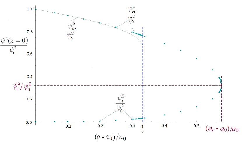
Figure 1: Found numerically by solving Eqs. (29,30) values of the dimensionless value of the hexatic order parameter $\psi^{2}/\psi_{m}^{2}\,$ at $z=0$ in the coexistence regime (sea-green circles) as a function of the dimensionless temperature deviation $(a-a_{0})/a_{0}$. The dark green solid line shows corresponding analytic result (Eq. (7)), and the blue vertical dash line shows the limit of the existence for this local minimum ($(a-a_{0})/a_{0}\leq\,1/3$).

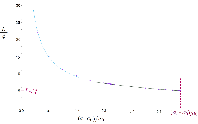
Figure 2: Found numerically by solving Eqs. (29,30,24) values of the dimensionless film thickness $L/\xi\,$ in the coexistence regime (lilac circles) as a function of the dimensionless temperature deviation $(a-a_{0})/a_{0}$. The azure dash line in the left shows corresponding analytic result (Eq. (59)). Green solid line (for $(a-a_{0})/a_{0}<\,(a_{c}-a_{0})/a_{0}$) is obtained by fitting with Eq. (69) the result near the point $\gamma=g_{c}$.

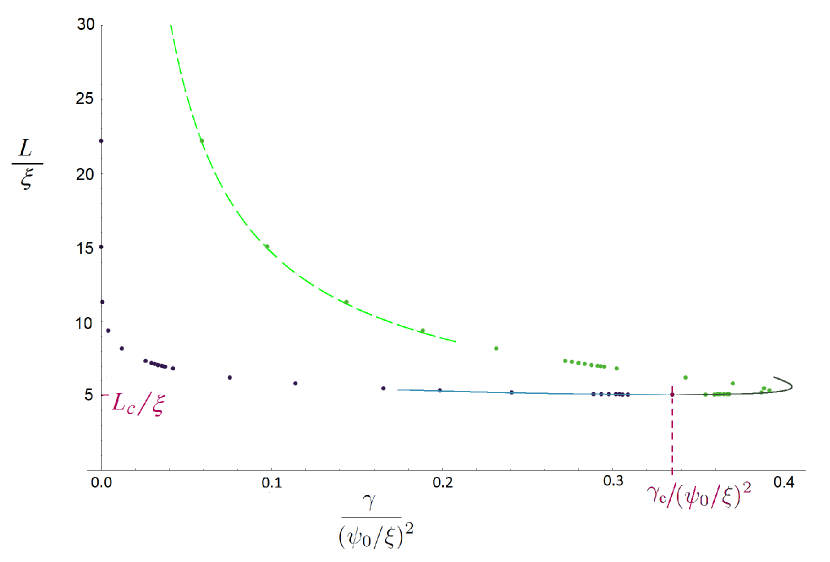
Figure 3: Numerical values (found by solving Eqs. (29,30), with Eq. (24) and using Eqs. (19,49)) for the dimensionless film thickness $L/\xi\,$ in the coexistence regime of $SmA$ (dark blue circles) and $HexB$ phase (green circles) presented as a function of the dimensionless variable $\gamma/(\psi_{0}/\xi)^{2}$. The last right numerical point corresponds to the condition $\partial\gamma/\partial L\,=0$. Corresponding analytical description according to the Eq. (59), using Eq. (49), is shown by the light green dash line in the left. Fitting, see Eqs. (69,70) in the vicinity of the point $\gamma=g_{c}$ is shown by blue solid line (for the $SmA$ phase, $\gamma\leq\,\gamma_{c}$) and by the dark green line (for the $HexB$ phase, $\gamma\geq\,\gamma_{c}$).

III.2 Model Landau functional

Here we exploit the model, introduced above, where the parameter $a$ is determined by the expansion (10) and the parameters $\lambda,\zeta$ are treated as constants, independent of temperature and chemical potential. In addition, we assume that the parameter $b$ is constant as well. Then one finds from Eqs. (15,18)

$$N_{A}=-\frac{\partial\Omega_{A}}{\partial\mu}=-\frac{\partial\Omega_{0}}{\partial\mu}-2\beta\int_{\psi_{A}}^{\psi_{s}}\frac{d\psi\ \psi^{2}}{\sqrt{g-\gamma_{A}}},$$ (31)

and an analogous expression for the hexatic phase.

Since $N_{A}=N$ at $T=T_{+}$ and $N_{H}=N$ at $T=T_{-}$, then the interval of the phase coexistence is determined by the condition $N_{H}(T_{-})=N_{A}(T_{+})$. According to Eq. (31), it is written as

$$\frac{\partial\Omega_{0}}{\partial\mu}(T_{-},\mu_{-})-\frac{\partial\Omega_{0}}{\partial\mu}(T_{+},\mu_{+})=2\beta\int_{\psi_{A}}^{\psi_{H}}\frac{d\psi\ \psi^{2}}{\sqrt{g_{+}-\gamma_{A}}}$$

$$+2\beta\int_{\psi_{H}}^{\infty}d\psi\ \psi^{2}\left(\frac{1}{\sqrt{g_{+}-\gamma_{A}}}-\frac{1}{\sqrt{g_{-}-\gamma_{H}}}\right),\qquad$$ (32)

where we, again, extended the integration up to infinity due to convergence of the integral. Here the parameters in $g_{+}$ and $\psi_{A}$ are taken at $T=T_{+}$ and the parameters in $g_{-}$ and $\psi_{H}$ are taken at $T=T_{-}$.

In our model $a$ is $L$-dependent parameter in the coexistence region. Therefore we obtain from the expression (10) $\alpha(T-T_{+})+\beta(\mu-\mu_{+})=0$. This means $\,g_{+}=g_{-}=g\,$, that is $a_{+}=a_{-}=a$ in the first order of the expansion of $a$ in the deviations $(T-T_{+})$, $(\mu-\mu_{+})$. In this way expanding the difference of the derivatives in Eq. (32) in $T_{+}-T_{-}$, $\mu_{+}-\mu_{-}$ and using the condition, we find the relation

$$\frac{L\Gamma}{2\beta}(T_{+}-T_{-})+\int_{\psi_{A}}^{\psi_{H}}\frac{d\psi\ \psi^{2}}{\sqrt{g-\gamma_{A}}}$$

$$+\int_{\psi_{H}}^{\infty}d\psi\ \psi^{2}\left(\frac{1}{\sqrt{g-\gamma_{A}}}-\frac{1}{\sqrt{g-\gamma_{H}}}\right)=0,$$ (33)

which determines the interval of the phase coexistence, see Fig. 4. The relation (33) can be rewritten as

$$\frac{L\Gamma}{\beta}(T_{+}-T_{-})+\frac{\partial\Delta\Phi}{\partial a}=0,$$ (34)

as a consequence of Eq. (28). These relations (33,34) are our main results in the work, and they are ready for further experimental inspection and theoretical analysis.

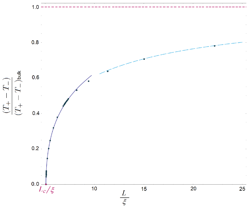
Figure 4: The temperature interval of the phase coexistence as a function of the dimensionless film thickness $L/\xi\,$, computed by solving numerically Eqs. (29), (30), (33) (dark blue points). Our theory result for the thick films (Eq. (64) is shown by the azure dash line in the right. Violet solid line (started from the point $L_{c}/\xi$) stands for the analytic solution to the Eqs. (34,46,47,69) in a vicinity of the point $a=a_{c}$.

III.3 Universal phase diagram

To get further insight into the nature of the equilibrium phase coexistence, it is convenient to utilize the dimensionless variables $a/a_{0}$ and $L/\xi$. Then we obtain a universal picture, independent of the concrete values of the model parameters, from the results of the previous subsection. Particularly, one can relate the variables $a/a_{0}$ and $L/\xi$. Although the solution of the above non-linear equations can be found only numerically, we one can formulate some general universal laws valid (within our model assumptions) in the equilibrium phase coexistence region. Namely, the relations (24) imply that in the coexistence regime the equation $\Xi(a,\gamma)=L$ should have at least two solutions. Already this deceptively simple observation restricts the values of our model parameters. Let us first look at the function $\Xi$.

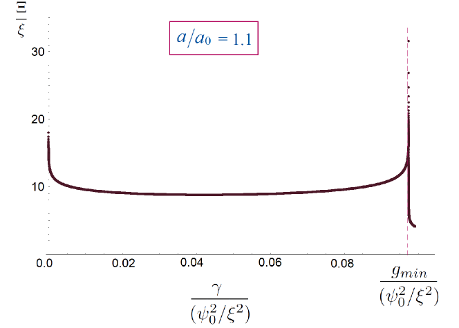
Figure 5: Computed from Eq.(23) for $a/a_{0}=1.1$ (i.e. for the case $1<a/a_{0}<4/3$) function $\Xi/\xi$ versus $\gamma/(\psi_{0}/\xi)^{2}$.

For small $\gamma$ the function $\Xi$ diverges logarithmically, see Fig. 5. If $1<a/a_{0}<4/3$, then the function $g(\psi)$ (19) has a minimum at non-zero $\psi$. Therefore the function $\Xi$ logarithmically diverges at $\gamma\to g_{min}$ where $g_{min}$ is the minimal value of the function $g$. Thus $\Xi$ has a minimum inside the interval $0<\gamma<g_{min}$, see Fig. 5. At $\gamma>g_{min}$ the function $\Xi$ monotonously decreases as $\gamma$ grows. At $a/a_{0}>4/3$ the minimum in the function $g(\psi)$ disappears and $\Xi$ becomes a regular function of $\gamma$. However, $\Xi$ remains a non-monotonic function of $\gamma$ (it has a minimum and a maximum, see Figs. 6-7 up to some critical value $a_{c}$, the value of $a_{c}/a_{0}$ is approximately equal to $1.5774$, see Fig. 7. At $a>a_{c}$ the function $\Xi(\gamma)$ becomes monotonic.

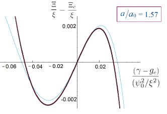
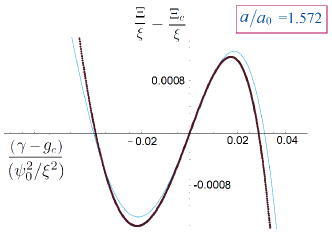
Figure 6: Comparison the numeric solution of Eq.(23) for ($\Xi/\xi$ as a function of $(\gamma-g_{c})/(\psi_{0}/\xi)^{2}$) ) with our theory analysis (Eq.(65)) (thin azure solid line). $a/a_{0}=1.57$ and $a/a_{0}=1.572$ (i.e. for the case $a/a_{0}>4/3$).

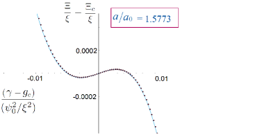
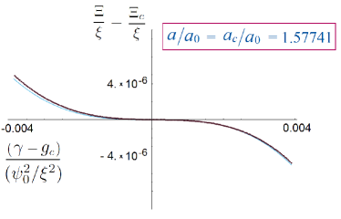
Figure 7: Comparison of numerically found by solving Eq. (23) $\Xi/\xi$ as a function of $(\gamma-g_{c})/(\psi_{0}/\xi)^{2}$ with analytical approximation Eq. (65) (thin azure solid line). $a/a_{0}=1.5773$ (i.e. for the case $a/a_{0}>4/3$) and $a/a_{0}=a_{c}/a_{0}=1.57741$.

Thus, at $a<a_{c}$ there are three solutions of the equation $\Xi=L$ in some interval of the film thickness $L$. The smallest by the value of $\psi$ solution corresponds to the $SmA$ phase, $\gamma=\gamma_{A}$. The next by its $\psi$ value solution corresponds to an unstable state. And finally the third solution with the biggest $\psi$ corresponds to the $HexB$ phase, $\gamma=\gamma_{H}$. In the limit $a\to a_{c}$ we find $\gamma_{A}\to\gamma_{H}$, and at $a>a_{c}$ there remains the only one solution of the equation $\Xi(a,\gamma)=L$. Then the equilibrium phase coexistence region shrinks to zero. This result which have been emanated from our analysis, states that the equilibrium phase coexistence is possible only in the interval $a_{0}<a<a_{c}$. Different values of $a$ correspond to the different values of the film thickness $L$, see Fig. 8. Found numerically value of $L_{c}/\xi$ is equal to $5.07$.

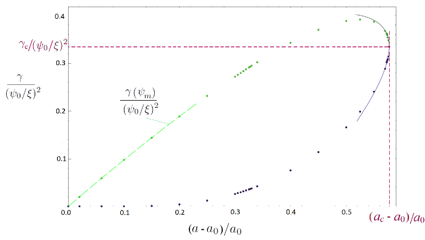
Figure 8: Numerically found by solving Eqs. (29,30), using Eq. (19, 49), values of $\gamma_{A}$ and $\gamma_{H}$ for the $SmA$ (blue circles) and $HexB$ phase (green circles) as a function of $(a-a_{0})/a_{0}$. Light green dash line represents the analytical dependence $\gamma(\psi_{m})/(\psi_{0}\,\xi^{-1})^{2}$. Using Eqs. (70) we fit the numerical data near the point $\gamma=g_{c}$. Solid lines dark blue for $SmA$ ($\gamma\leq\,\gamma_{c}$) and dark green for $HexB$ phase ($\gamma\geq\,\gamma_{c}$).

III.4 Thick films

In this subsection we analyze the case of large film thickness, $L\gg\xi$. The limit has been discussed at the semi-quantitatively level in ZK18 . Here we present the quantitative theory. For the thick films naturally the deviations of the film properties from the bulk ones are relatively weak. Particularly, the value of the parameter $a$ is close to its bulk value $a_{0}$, $a-a_{0}\ll a_{0}$. It follows from the relations (24) that at $L\gg\xi$ the integral (23) is anomalously large. It enables us to develop the consistent analytical procedure to study the surface effects in the equilibrium phase coexistence regime.

Let us turn to the hexatic phase. The value of $\psi$ in the hexatic phase, $\psi_{H}$, is close to $\psi_{m}$, that corresponds to the minimum of $g$, see Eq. (7). The main contribution to the integral (23) stems from the vicinity of $\psi_{m}$. Near $\psi_{m}$ the function $g$ can be approximated as

$$g=\frac{\psi_{0}^{2}}{b}\left[a-a_{0}+\frac{\lambda}{3}(\psi-\psi_{m})^{2}\right].$$ (35)

Starting from Eq. (35) and using Eqs. (23,24), we find with the logarithmic accuracy

$$\frac{L}{\xi}=\ln\frac{\psi_{0}}{\psi_{H}-\psi_{m}}.$$ (36)

Thus, $\psi_{H}-\psi_{m}$ is exponentially small in $L/\xi$.

Let us now turn to the $SmA$ phase. At $L\gg\xi$ the main contribution to the integral (23) comes from the small $\psi$, where $g\approx a\psi^{2}/b$. Calculating the integral with the logarithmic accuracy, one obtains

$${L}/{\xi}=2\ln(\psi_{0}/\psi_{A}).$$ (37)

We conclude from Eq. (37), that $\psi_{A}$ is exponentially small in $L/\xi$.

Now we use the condition $\Delta\Phi=0$, see Eq. (25), to find $a$ at a given $L$. We can substitute into Eq. (25) $\psi_{A}=0$ and $\psi_{H}=\psi_{m}$. In the main approximation one obtains

$$\frac{a_{0}}{a-a_{0}}+\ln\frac{a_{0}}{a-a_{0}}=\frac{L}{\xi}.$$ (38)

We see, that $(a-a_{0})/a_{0}$ is a power of $\xi/L$, that justifies the substitution $\psi_{A}\to 0$ and $\psi_{H}-\psi_{m}\to 0$ since the quantities are exponentially small.

Note that for the $SmA$ phase there is an additional logarithmic contribution to the integral in Eq. (23), related to a vicinity of the minimum of $g(\psi)$, containing $\ln[a_{0}/(a-a_{0})]$. As it follows from Eq. (38), the logarithm is $\ln(L/\xi)$. Therefore the contribution is irrelevant in comparison with $L/\xi$ in the left hand side of Eq. (37).

Now we rewrite Eq. (33) as

$$\frac{L\Gamma}{2\beta}(T_{+}-T_{-})+\int_{0}^{\psi_{m}}\frac{d\psi\ \psi^{2}}{\sqrt{g}}$$

$$+\int_{\psi_{m}}^{\infty}d\psi\ (\psi^{2}-\psi_{m}^{2})\left(\frac{1}{\sqrt{g}}-\frac{1}{\sqrt{g-\gamma_{H}}}\right)$$

$$+\psi_{m}^{2}\int_{\psi_{m}}^{\infty}\frac{d\psi}{\sqrt{g}}-\psi_{m}^{2}\int_{\psi_{H}}^{\infty}\frac{d\psi}{\sqrt{g-\gamma_{H}}}=0,$$ (39)

where we substituted $\psi_{A}=0$, $\psi_{H}=\psi_{m}$. The last term in Eq. (39) is equal to $\psi_{m}^{2}L/2$, in agreement with Eq. (24).

In the main approximation we find

$$\frac{\Gamma}{\beta\psi_{0}^{2}}(T_{+}-T_{-})=1-\frac{\xi}{L}\ln\frac{L}{\xi},$$ (40)

where we used Eq. (38). The expression (40) gives the first correction to the bulk expression (14). The contributions leading to the logarithmic factor in the Eq. (40) were missed in the work ZK18 . Therefore the expression for the temperature width of the phase coexistence region presented in ZK18 can be used only for qualitative interpretation of the data (note however that in terms of numeric values for the range of the film thicknesses considered in ZK18 , the logarithmic factor is almost irrelevant). Nevertheless the logarithmic factor is very important conceptually. Thanks to this factor we are in the position to perform consistently our calculations with logarithmic accuracy (see, however, the appendices with higher order corrections included). Besides it allows us to distinguish found above law for the temperature width of the coexistence region, from regular (existing in any system) finite size corrections which scales as $\xi/L$. The fact that $\psi_{A}$ and $\psi_{H}-\psi_{m}$ are exponentially small, enables us to find analytically next terms of the expansion in the parameter $\xi/L$ in the expression for $T_{+}-T_{-}$. The corresponding analysis is placed into Appendix A, see also Figs. 2, 3.

III.5 Thin films

Being interested in thin films, we consider the case $a>4/3a_{0}$. Then the quantity $\Xi$ (23) has no singularities, as a function of $\gamma$. However, at $a<a_{c}$ it is still a non-monotonic function of $\gamma$. At $a=a_{c}$ the function $\Xi$ (23) has a point $\gamma=g_{c}$, where both, $\partial\Xi/\partial\gamma$ and $\partial^{2}\Xi/\partial\gamma^{2}$ are equal to zero.

In the vicinity of the point the quantity $\Xi$ can be approximated as

$$\frac{\Xi}{\xi}=\frac{\Xi(a,y_{c})}{\xi}-A(y-y_{c})^{3}-B\frac{a-a_{c}}{a_{0}}(y-y_{c}),$$ (41)

where $\gamma=(\psi_{0}^{2}/\xi^{2})y$ and $A,B$ are dimensionless constants. Their numerical values are $A=82.1362$, $B=17.6392$. Exploiting Eq. (26), one finds from Eq. (41)

$$\frac{\xi\Delta\Phi}{\psi_{0}^{2}}=\left[\frac{\Xi(a,y_{c})}{\xi}-\frac{L}{\xi}\right](y_{H}-y_{A})$$

$$-\frac{A}{4}\left[(y_{H}-y_{c})^{4}-(y_{A}-y_{c})^{4}\right]$$

$$-\frac{B}{2}\frac{a-a_{c}}{a_{0}}\left[(y_{H}-y_{c})^{2}-(y_{A}-y_{c})^{2}\right].$$ (42)

Now we can find the equilibrium values of the parameters that are determined by the conditions (24) and $\Delta\Phi=0$. The conditions (24) are written as

$$\Xi(a,y_{c})/\xi-L/\xi\qquad$$

$$=A(y_{H}-y_{c})^{3}+B\frac{a-a_{c}}{a_{0}}(y_{H}-y_{c})$$

$$=A(y_{A}-y_{c})^{3}+B\frac{a-a_{c}}{a_{0}}(y_{A}-y_{c}).$$ (43)

Equating then $\Delta\Phi$ to zero, we find from Eqs. (42) and (43)

$$L=\Xi(a,y_{c}),\qquad$$ (44)

$$y_{H}-y_{c}=\sqrt{B(a_{c}-a)/(Aa_{0})},$$

$$y_{A}-y_{c}=-\sqrt{B(a_{c}-a)/(Aa_{0})}.$$ (45)

Thus the equilibrium branch of the curve $y_{A}(a),y_{H}(a)$ near the point $a_{c},y_{c}$ is a parabola.

Since in the equilibrium the derivatives of $\Delta\Phi$ over $\gamma_{A}=(\psi_{0}^{2}/\xi^{2})y_{A}$ and $\gamma_{H}=(\psi_{0}^{2}/\xi^{2})y_{H}$ are zero, we find in the main approximation from Eq. (42)

$$\frac{\partial\Delta\Phi}{\partial a}=2\frac{\psi_{0}^{2}}{\xi^{2}}\frac{\partial\Xi}{\partial a}\sqrt{\frac{B(a_{c}-a)}{Aa_{0}}},$$ (46)

at the equilibrium curve. Here the derivative $\partial\Xi/\partial a$ is taken at $y=y_{c}$. We conclude that

$$\frac{\partial\Delta\Phi}{\partial a}\propto(a_{c}-a)^{1/2},$$ (47)

that is the derivative tends to zero as $a\to a_{c}$, see Fig. 9. Thus, in the agreement with Eqs. (34) the width of the equilibrium phase coexistence region shrinks, $T_{+}-T_{-}\propto(a_{c}-a)^{1/2}$ as $a\to a_{c}$, see Figs. 4, 10. A similar procedure can be used to calculate the higher order terms in $a-a_{c}$, $y-y_{c}$ to the expansion (41). Technical details and final results are presented in Appendix B, see also Figs. 2, 3.

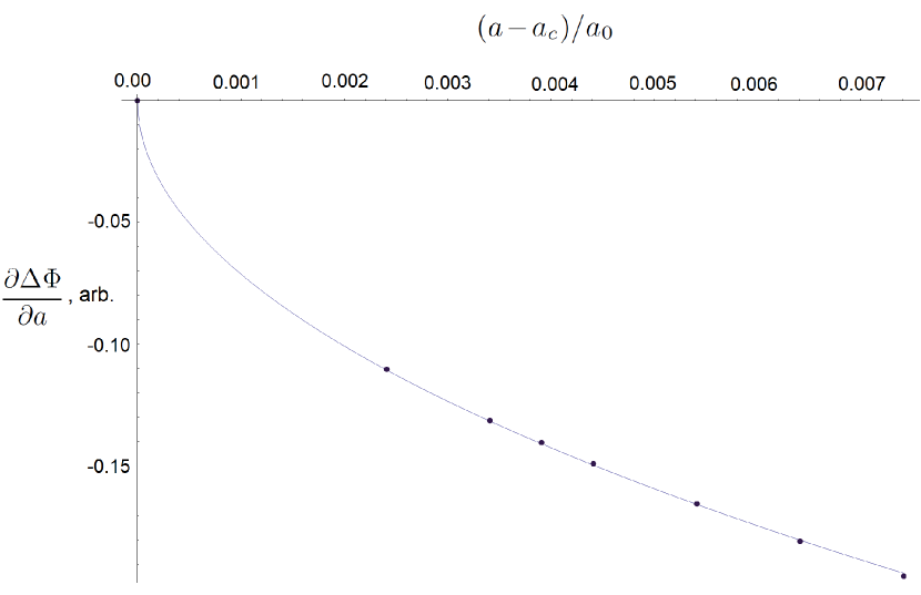
Figure 9: Comparison of our numeric results (solution to the Eq.(28) for ${\partial\Delta\Phi}/{\partial a}\,$ versus $(a-a_{c})/a_{0}$ ) in the coexistence regime (dark blue circles) with analytic theory (Eq. (47)) near the point $a=a_{c}$ (blue solid line).

IV Conclusion

In summary, we developed the theory describing features of the free standing smectic films in the temperature range where the equilibrium phase coexistence $SmA$ – $HexB$ occurs. Our results explain how the surface induced ordering reduces the width of the equilibrium phase coexistence region. Quite remarkably the width shrinks to zero, where the film thickness $L$ becomes of the order of the hexatic correlation length. The behavior of the film at $L\to L_{c}$ resembles the classical gas-liquid critical point, where the coexisting phases become indistinguishable. Our analysis of the surface-bulk ordering interplay predicts exclusive laws for the equilibrium phase coexistence range, in terms of the reduced parameters. The described phenomena (and the calculated specific relations between the parameters) are universal, appropriately rescaled our main predictions depend only on a few dimensionless parameters. Thus we arrived at the universal picture in terms of the reduced parameters.

Let us stress that our crucial assumption, that the $SmA$ – $HexB$ transition is close to the tricritical point, is strongly supported by the existing experimental data. For example, see Refs. JV95 ; HK97 ; RD05 ; MP13 ; ZK18 , that demonstrates weak first order phase transitions. Moreover, the measured critical exponents (for the specific heat and for the order parameter) are close to those for the tricritical point JV95 ; HK97 ; RD05 ; MP13 . Therefore our theory is applicable to all the materials, and our predictions (the finite temperature range for the equilibrium phase coexistence, the film thickness as the parameter governing the width of the coexistence region and universal laws for the width dependence on the system parameters) hold.

We neglected fluctuations of the order parameter. It is well known, that near the tricritical point fluctuations provide logarithmic corrections to the mean-field values. Since, in accordance with our scheme, in the range of the equilibrium phase coexistence the control parameter $a$ varies in a relatively narrow interval (on the order of the bulk value $a_{0}$), the logarithmic renormalization of the coefficients is not essential for our consideration. However, if the reducing film thickness approaches the critical value $L_{c}$, then the smectic and the hexatic states become indistinguishable, signaling about a special critical point. This special critical point is basically similar to the conventional liquid – gas critical point, where fluctuations of the two-component hexatic order parameter (modulus and phase) are relevant (see PP79 in addition to LL80 ; ST87 ; AN91 ). We defer an investigation of the point for a future work.

To illustrate how our theory works we re-analyze the experimental data presented in Ref. ZK18 for the $SmA$ – $HexB$ coexistence in the free-standing film of the 54COOBC material. Measured in ZK18 the temperature width $\Delta T$ of the phase coexistence region at different film thickness can be reasonably described by our theory. The comparison suggests also that these experimental data correspond to the regime of the intermediate film thicknesses (in-between described analytically the thick and thin films limits). We presented in Fig. 10 (similarly as it has been done in Fig. 2) our numeric solution to Eqs. (29,30), and Eq. 24).

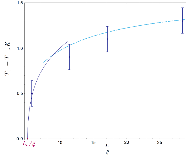
Figure 10: Borrowed from ZK18 experimental data on the temperature range $\Delta T$ of the $SmA$ and $HexB$ phase coexistence as a function of the dimensionless film thickness $L/\xi\,$ (on cooling, shown by dark blue circles). Our analytical description of the data by Eq. (64) for the thick films is shown by the azure dash line in the right. In numeric computation we used the following fitting parameters: $\xi=3.5\cdot 10^{-7}$ m, ${\beta\psi_{0}^{2}}/\Gamma=1.6$. Our results near the point $a=a_{c}$ (the violet solid line) is plotted by solving Eqs. (34,46,46,47,69).

In this work we had deal only with $SmA$ – $HexB$ phase transition in a vicinity of the tricritical point, characterized by the two-component (complex) order parameter. Generally, our theory can be applied to other orientation phase transitions in smectics (provided the state is close to a tricritical point). For example, it is applicable to the transition between the untilted $SmA$ and the tilted $SmC$ states. However, the explicit expressions require some modifications. Namely, one has to include into consideration, uniaxial orientational anisotropy within the smectic layers (to compare with the hexagonal symmetry of the $HexB$ layers), and, more important, induced by cooperative molecular tilting the layer thickness variation at the transition.

Our theory can be adjusted to describe the paraelectric – ferroelectric phase transitions in the solid films as well, where the transition is close to a tricritical point (see, e.g., Gerzanich ; Strukov for the case of thin ceramic ferroelectric films). Furthermore for the thin ferroelectric films surface ordering occurs prior the bulk one, and it yields to a sort critical point, mentioned in Scott ; Duiker ; Qu . To modify our theory for the ferroelectric solid films, one has to include elastic energy, long-range dipolar forces, domain structures and so on. Notes also that the equilibrium phase coexistence, tricritical behavior, and the film finite thickness effects are very common in nature, not only for the smectics or the ferroelectrics, but for spin-density waves, charge density waves, adsorbed atoms as well.

A remarkable peculiarity of Landau theory is that it is a powerful tool for description of different systems in terms of the order parameter irrespective of its microscopic nature. The system properties depend solely on the system dimension, symmetry, and on the number of the components of the order parameter. Similarity in the description can be even more close if one considers quasi two-dimensional layered structures, such as high-temperature superconductors with puzzling properties. What can be useful for us considering other systems? The matter is that in the smectic liquid crystals, unlike superconductors and superfluids, not only both components of the order parameter have a transparent physical nature, but also the fields conjugated to the modulus and phase have realistic physical sources (e.g., uniaxial pressure or electric and magnetic fields). This cannot be said about superconducting gap and superfluid density for which there is no conjugated physical field. It is tempting to use smectic phases for modeling of different unusual superstructures forming in superconductors and superfluids. To the same point, the idea (we are advocating here) on the bulk - surface orderings correspondence in smectic films, became recently very popular with a number of fascinating applications in several branches of physics, like holographic principle in high energy physics, or in topological insulators (see, e.g., BO02 ; HK10 ).

Appendix A

Here we analyze the case of thick films, $L\gg\xi$. Then $a$ is close to $a_{0}$. The system of equations can be brought in a more elegant form (ready for numerics) by introducing dimensionless variables

$$\varpi=a/a_{0}-1,\quad x=\psi^{2}/\psi_{0}^{2},$$ (48)

one obtains

$$g=(\psi_{0}/\xi)^{2}x(1+\varpi-2x+x^{2}).$$ (49)

The parameter $\varpi>0$ is small in our case. The quantity $g$ (49) has the minimum at $x=x_{m}$, where

$$x_{m}=\frac{2}{3}\left(1+\frac{1}{2}\sqrt{1-3\varpi}\right)<1.$$ (50)

As we explained, in the case $L/\xi\gg 1$ both, $\psi_{A}$ and $\psi_{H}-\psi_{m}$, are exponentially small in $L/\xi$. Therefore at analyzing effects, power in $\xi/L$, one can put $\psi_{A}=0$, $\psi_{H}=\psi_{m}=\psi_{0}\sqrt{x}_{m}$. Then one finds from Eq. (20)

$$\frac{\xi}{b\psi_{0}^{2}}\Phi_{A}=\varphi_{A},\qquad$$ (51)

$$\frac{\xi}{b\psi_{0}^{2}}\Phi_{H}=2x_{m}^{2}(1-x_{m})\frac{L}{\xi}+\varphi_{H}.$$ (52)

The dimensionless quantities $\varphi_{A}$ and $\varphi_{H}$ are defined as

$$\varphi_{A}=2\int_{0}^{s}{dx}\sqrt{x^{2}-2x+1+\varpi}$$

$$=(s-1)(s^{2}-2s+1+\varpi)^{1/2}+\sqrt{1+\varpi}$$

$$-\varpi\ln\frac{1-s+(s^{2}-2s+1+\varpi)^{1/2}}{1+\sqrt{1+\varpi}},$$ (53)

and

$$\varphi_{H}=2\int_{x_{m}}^{s}\frac{dx}{\sqrt{x}}\sqrt{x-2(1-x_{m})}\,(x-x_{m})=$$

$$(s-x_{m}-1)\sqrt{s(s-2+2x_{m})}+\sqrt{x_{m}(3x_{m}-2)}$$

$$+2\varpi\ln\frac{\sqrt{s}+\sqrt{s-2(1-x_{m})}}{\sqrt{x_{m}}+\sqrt{3x_{m}-2}},$$ (54)

where the subscript $s$ corresponds to the surface value of the order parameter.

Using Eqs. (53,54), one can easily calculate

$$\lim_{s\to\infty}(\varphi_{A}-\varphi_{H})=\sqrt{1+\varpi}-\sqrt{x_{m}(3x_{m}-2)}$$

$$+x_{m}-\varpi\ln\frac{2(\sqrt{1+\varpi}\,-1)}{(\sqrt{x_{m}}+\sqrt{3x_{m}-2})^{2}}.$$ (55)

Therefore the condition $\Delta\Phi=0$ reads as

$$\sqrt{1+\varpi}-\sqrt{x_{m}(3x_{m}-2)}+x_{m}$$

$$-\varpi\ln\frac{2(\sqrt{1+\varpi}\,-1)}{(\sqrt{x_{m}}+\sqrt{3x_{m}-2})^{2}}$$

$$=2x_{m}^{2}(1-x_{m})\frac{L}{\xi}.$$ (56)

This equation relates $\xi/L$ and $\varpi$.

Now we turn to the relation (39) that can be rewritten as

$$\frac{\Gamma}{\beta\psi_{0}^{2}}(T_{+}-T_{-})+\frac{\xi}{L}\int_{0}^{s}\frac{dx}{\sqrt{x^{2}-2x+1+\varpi}}$$

$$-\frac{\xi}{L}\int_{x_{m}}^{s}\frac{dx}{\sqrt{x^{2}-2(1-x_{m})x}}-x_{m}=0.$$ (57)

The integrals here are

$$\int_{0}^{s}\frac{dx}{\sqrt{x^{2}-2x+1+\varpi}}=\ln\frac{s-1+\sqrt{s^{2}-2s+\varpi}}{\sqrt{1+\varpi}\,-1},$$

$$\int_{x_{m}}^{s}\frac{dx}{\sqrt{x^{2}-2(1-x_{m})x}}=2\ln\frac{\sqrt{s}+\sqrt{s-2+2x_{m}}}{\sqrt{x_{m}}+\sqrt{3x_{m}-2}}.$$

Substituting the expressions into Eq. (57) and passing to the limit $s\to\infty$, one obtains

$$\frac{\Gamma(T_{+}-T_{-})}{\beta\psi_{0}^{2}}+\frac{\xi}{L}\ln\frac{(\sqrt{x_{m}}+\sqrt{3x_{m}-2})^{2}}{2(\sqrt{1+\varpi}\,-1)}=x_{m}.\quad$$ (58)

The equation relates $\xi/L$ and $T_{+}-T_{-}$.

The expressions (50,56,58) admit a regular expansion in $\varpi$. Keeping zero and first terms of the expansion, we get

$$\frac{1}{\varpi}+\ln\frac{4}{\varpi}+\frac{5}{4}=\frac{L}{\xi},$$ (59)

$$\frac{\Gamma(T_{+}-T_{-})}{\beta\psi_{0}^{2}}=\frac{\xi}{L\varpi}+\frac{\xi}{L}-\frac{\varpi}{4}.$$ (60)

Taking into account only the main logarithmic term, we reproduce Eqs. (38,40). In the next order in $\varpi$ one finds the relations

$$\frac{1}{\varpi}+(1+\frac{\varpi}{4})\,\ln\frac{4}{\varpi}+\frac{5}{4}+\frac{\varpi}{16}=\frac{L}{\xi},$$ (61)

$$\frac{\Gamma(T_{+}-T_{-})}{\beta\psi_{0}^{2}}=\frac{\xi}{L\varpi}+\frac{\xi}{L}+\frac{3\varpi}{8}\frac{\xi}{L}-\frac{\varpi}{4}-\frac{\varpi^{2}}{4}.$$ (62)

Expressing $\varpi$ via $\xi/L$ from Eq. (61), we obtain in the same approximation

$$\varpi=\frac{\xi}{L}+\left(\frac{\xi}{L}\right)^{2}\left(\ln\frac{4L}{\xi}+\frac{5}{4}\right)$$

$$+\left(\frac{\xi}{L}\right)^{3}\left[\left(\ln\frac{4L}{\xi}\right)^{2}+\frac{7}{4}\ln\frac{4L}{\xi}+\frac{3}{8}\right],$$ (63)

the function ${L}/{\xi}$ versus $\varpi$ is presented in Fig. 2. Substituting the expression (63) into Eq. (62), we finally find

$$\frac{\Gamma(T_{+}-T_{-})}{\beta\psi_{0}^{2}}=1-\frac{\xi}{L}\left(\ln\frac{4L}{\xi}+\frac{1}{2}\right)$$

$$+\left(\frac{\xi}{L}\right)^{2}\left(\frac{1}{2}\ln\frac{4L}{\xi}+1\right),$$ (64)

in the second order in $\xi/L$. We plot the corresponding dependence of $T_{+}-T_{-}$ on the dimensionless film thickness $L/\xi\,$ in Fig. 4.

Appendix B

Here we analyze in more detail the case where $L$ is close to $L_{c}$ and the coexistence region is rather narrow in its width. Then one should start from the expression (41), correct near the point $a_{c},y_{c}$. We discuss next corrections to the expression (41). The modified expression can be written as

$$\frac{\Xi}{\xi}=\frac{\Xi(a,y_{c})}{\xi}-A(y-y_{c})^{3}-B\frac{a-a_{c}}{a_{0}}(y-y_{c})$$

$$+C(y-y_{c})^{4}+D\frac{a-a_{c}}{a_{0}}(y-y_{c})^{2},\qquad$$ (65)

$$\frac{\Xi(a,y_{c})}{\xi}=\frac{\Xi_{c}}{\xi}+A_{1}\frac{a-a_{c}}{a_{0}}+B_{1}\left(\frac{a-a_{c}}{a_{0}}\right)^{2},\quad$$ (66)

where $A,B,D,C,A_{1},B_{1}$ are dimensionless parameters. The corrections with the coefficients $C,D$ contain an extra power of $y-y_{c}$ in comparison with the main terms with the coefficients $A,B$. The parameters $D,C,A_{1},B_{1}$ can be found numerically, they are $D=-45.6325$, $C=-724.459$, $A_{1}=-4.81157$, $B_{1}=14.4096$.

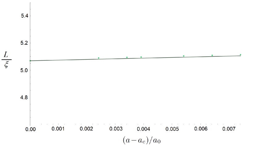
Figure 11: Comparison of the numeric results for $L/\xi\,$ (light green circles) versus $a-a_{c}$ with their analytic counterparts given by Eq.((69)) near the point $a=a_{c}$. Branch corresponding to the Eq.(69) is shown by the dark green solid line.

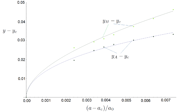
Figure 12: Comparison of the numeric results for $\,y_{H}-y_{c}\,$ (light green circles) and $\,y_{A}-y_{c}\,$ (blue circles) versus $a-a_{c}$ with analytic ones given by Eqs.((70)) near the point $a=a_{c}$. Curves corresponding to the Eqs. (70) are shown by the solid lines (upper dark green for $HexB$ phase and bottom blue for $SmA$) .

The next step is in generalizing Eq. (42)

$$\frac{\xi\Delta\Phi}{\psi_{0}^{2}}=\left[\frac{\Xi(a,y_{c})}{\xi}-\frac{L}{\xi}\right](y_{H}-y_{A})$$

$$-\frac{A}{4}\left[(y_{H}-y_{c})^{4}-(y_{A}-y_{c})^{4}\right]$$

$$-\frac{B}{2}\frac{a-a_{c}}{a_{0}}\left[(y_{H}-y_{c})^{2}-(y_{A}-y_{c})^{2}\right]$$

$$+\frac{C}{5}\left[(y_{H}-y_{c})^{5}-(y_{A}-y_{c})^{5}\right]$$

$$+\frac{D}{3}(\varpi-\varpi_{c})\left[(y_{H}-y_{c})^{3}-(y_{A}-y_{c})^{3}\right].$$ (67)

Now we can find the equilibrium values of the parameters that are determined by the conditions (24) and $\Delta\Phi=0$. The conditions (24) are written as

$$\Xi(a,y_{c})/\xi-L/\xi$$

$$=A(y_{H}-y_{c})^{3}+B(\varpi-\varpi_{c})(y_{H}-y_{c})$$

$$+C(y_{H}-y_{c})^{4}+D\frac{a-a_{c}}{a_{0}}(y_{H}-y_{c})^{2}$$

$$=A(y_{A}-y_{c})^{3}+B\frac{a-a_{c}}{a_{0}}(y_{A}-y_{c})$$

$$+C(y_{A}-y_{c})^{4}+D\frac{a-a_{c}}{a_{0}}(y-y_{c})^{2}.$$ (68)

The expressions generalize Eq. (43). The condition $\Delta\Phi=0$ gives the equation following from Eq. (67).

To have a regular expansion (perturbation theory) we assume the higher order corrections to be small. Then we find

$$\frac{L}{\xi}-\frac{\Xi(a,y_{c})}{\xi}=\left(\frac{C}{5}-\frac{DA}{3B}\right)\left(\frac{B(a-a_{c})}{Aa_{0}}\right)^{2},$$ (69)

$$y_{H},y_{A}=y_{c}\pm\sqrt{\frac{B(a-a_{c})}{Aa_{0}}}$$

$$-\left(\frac{3C}{5A}-\frac{2D}{3B}\right)\frac{B}{A}\frac{a-a_{c}}{a_{0}},$$ (70)

instead of Eqs. (44,45). The applicability condition of the expressions implies that the corrections to $y_{H},y_{A}$ are small in comparison with the main contribution. Comparing the expression (69) with Eq. (66), we conclude, that $L$ is expanded over integer powers of $(a-a_{c})/{a_{0}}$. Our numeric results, shown in Figs. 11, 12 are in agreement with presented above analytic expansion, see Eqs. (69,70).

References

- (1) W.H. de Jeu, B.I. Ostrovskii, A.N. Shalaginov, Rev. Mod. Phys., 75, 181 (2003).
- (2) P. Oswald, P. Pieranski, Smectic and columnar liquid crystals, Taylor and Francis Group, Boca Raton (2006).
- (3) I.A. Zaluzhnyy, R.P. Kurta, N. Mukharamova, Young Yong Kim, R.M. Khubbutdinov, D. Dzhigaev, V.V. Lebedev, E.S. Pikina, E.I. Kats, N.A. Clark, M. Sprung, B.I. Ostrovskii, I.A. Vartanyants, Physical Review E, 98, 052703 (2018).
- (4) S. Stoebe, P. Mach, and C.C. Huang, Phys. Rev. Lett. 73, 1384 (1994).
- (5) E.I. Demikhov, V.K. Dolganov and K.P. Meletov, Phys. Rev. E 52, R1285 (1995).
- (6) W.H. de Jeu, B.I. Ostrovskii, A.N. Shalaginov, Rev. Mod. Phys. 75, 81 (2003).
- (7) F. Picano, P. Oswald, and E. Kats, Phys. Rev. E 63, 021705 (2001).
- (8) S. Stoebe, and C.C. Huang, Int. J. Mod. Phys. B 9, 2285 (1995).
- (9) E. I. Demikhov, Mol. Cryst. Liq. Cryst. Sci. Technol., Sect. A 265, 403 (1995).
- (10) E.I. Demikhov, V.K. Dolganov and K.P. Meletov, Phys. Rev. E 52, R1285 (1995).
- (11) P.M. Johnson, P. Mach, E.D. Wedell, F. Lintgen, M. Neubert, and C. C. Huang, Phys. Rev. E 55, 4386 (1997).
- (12) W.H. de Jeu, A. Fera, and B.I. Ostrovskii, Eur. Phys. J. E 15, 61 (2004).
- (13) Ch. Bohley and R. Stannarius, Soft Matter, 4, 683 (2008).
- (14) E.S. Pikina, B.I. Ostrovskii and W.H. de Jeu, Eur. Phys. J. E 38: 13 (2015).
- (15) E.S. Pikina and B.I. Ostrovskii, Eur. Phys. J. E 40: 24 (2017).
- (16) A.J. Jin, M. Veum, T. Stoebe, C.F. Chou, J.T. Ho, S.W. Hui, V. Surendranath, C.C. Huang, Phys. Rev. Lett., 74, 4863 (1995).
- (17) H. Haga, Z. Kutnjak, G.S. Iannacchione, S. Qian, D. Finotello, C.W. Garland, Phys. Rev. E, 56, 1808 (1997).
- (18) B.Van Roie, K. Denolf, G. Pitsi, J. Thoen, Eur. Phys. Journal, E, 16, 361 (2005).
- (19) F. Mercuri, S. Paolini, M. Marinelli, R. Pizzoferrato, U. Zammit, J. Chem. Phys. 138, 074903 (2013).
- (20) A.J. Jin, M.Veum, T. Stoebe, C.F. Chou, J.T. Ho, S.W. Hui, V. Surendranath, C.C. Huang, Phys. Rev. E, 53, 3639 (1996).
- (21) I.A. Zaluzhnyy, R.P. Kurta, E.A. Sulyanova, O.Yu. Gorobtsov, A.G. Shabalin, A.V. Zozulya, A.P. Menushenkov, M. Sprung, A. Krowczynski, E. Gorecka, B.I. Ostrovskii, I.A. Vartanyants, Soft Matter, 13, 3420 (2017).
- (22) L.D. Landau, E.M. Lifshitz, Course of Theoretical Physics, Statistical Physics, Part 1, Pergamon Press, New York (1980).
- (23) K. Huang, Statistical Mechanics, 2nd edition, John Wiley and Sons, Montreal (1987).
- (24) P. Oswald, P. Pieranski, F. Picano, R. Holyst, Phys. Rev. Lett., 88, 015503 (2001).
- (25) P. Oswald, G. Poy, Eur. Phys. Journal E, 41, 73 (2018).
- (26) H.E. Stanley, Introduction to phase transitions and critical phenomena, Oxford University Press, New York (1987).
- (27) M.A. Anisimov, Critical phenomena in liquids and liquid crystals, Gordon and Breach, Philadelphia (1991).
- (28) P.M. Chaikin, T.C. Lubensky, Principles of condensed matter physics, Cambridge University Press, Cambridge, 2000.
- (29) P.G. de Gennes and J. Prost, The Physics of Liquid Crystals, Claredon Press, Oxford, 1993.
- (30) E.V. Gurovich, E.I. Kats, V.V. Lebedev, ZhETF 100, 855 (1991) [Sov. Phys. JETP 73, 473 (1991)].
- (31) Chia-Fu Chou, A.J. Anjun, S.W. Hui, C.C. Huang, J.T. Ho, Science, 280, 1424 (1998).
- (32) T. Stoebe, R. Geer, C.C. Huang, J.W.Goodby, Phys. Rev. Lett., 69, 2090 (1992).
- (33) R. Geer, T. Stoebe, C.C. Huang, Phys. Rev. E, 48, 408 (1993).
- (34) A.Z. Patashinskii, V.L. Pokrovskii, Fluctuation Theory of Phase Transitions, Pergamon Press, New York, 1979.
- (35) K.G. Wilson, Phys. Rev. B. 4, 3174 (1971).
- (36) K.G. Wilson, Phys. Rev. B. 4, 3184 (1971).
- (37) R. Bousso, Rev. Mod. Phys., 74, 825 (2002).
- (38) M.Z. Hasan, C.L. Kane, Rev. Mod. Phys., 82, 3045 (2010).
- (39) E.I. Gerzanich, V.M. Fridkin, Pis’ma Zh. Eksp. Teor. Fiz. 8 553 (1968) [JETP Lett. 8 337 (1968)].
- (40) B.A. Strukov, M. Amin, V.A. Koptsik, Phys. Status Solidi 27 (1968).
- (41) J.F. Scott, M.-S. Zhang, R.B. Godfrey, C. Araujo, and L. McMillan, Phys. Rev. B 35, 4044 (1987).
- (42) J.F. Scott, H.M. Duiker, P.D. Beale and B. Pouligny, K. Dimmler, M. Parris, D. Butler and S. Eaton, Physica B 150, 160 (1988).
- (43) B.D. Qu, P.L. Zhang, Y.G. Wang, C.L. Wang, W.L. Zhong, Ferroelectrics 152, 219 (1994).