Concentration inequalities in spaces of random configurations with positive Ricci curvatures

Linyuan Lu University of South Carolina, Columbia, SC 29208, (lu@math.sc.edu). This author was supported in part by NSF grant DMS-1600811.    Zhiyu Wang University of South Carolina, Columbia, SC 29208, (zhiyuw@math.sc.edu). This author was supported in part by NSF grant DMS-1600811.
Abstract

In this paper, we prove an Azuma-Hoeffding-type inequality in several classical models of random configurations, including the Erdős-Rényi random graph models $G(n,p)$ and $G(n,M)$, the random $d$-out(in)-regular directed graphs, and the space of random permutations. The main idea is using Ollivier’s work on the Ricci curvature of Markov chairs on metric spaces. Here we give a cleaner form of such concentration inequality in graphs. Namely, we show that for any Lipschitz function $f$ on any graph (equipped with an ergodic random walk and thus an invariant distribution $\nu$) with Ricci curvature at least $\kappa>0$, we have

$$\nu\left(|f-E_{\nu}f|\geq t\right)\leq 2\exp\left(-\frac{t^{2}\kappa}{7}\right).$$

1 Introduction

One of the main tools in probabilistic analysis and random graph theory is the concentration inequalities, which are meant to bound the probability that a random variable deviates from its expectation. Many of the classical concentration inequalities (such as those for binomial distributions) provide best possible deviation results with exponentially small probabilistic bounds. Such concentration inequalities usually require certain independence assumptions (e.g., the random variable is a sum of independent random variables). For concentration inequalities without the independence assumptions, one popular approach is the martingale method. A martingale is a sequence of random variables $X_{0},X_{1},\ldots,X_{n}$ with finite means such that $E[X_{i+1}|X_{i},X_{i-1},\ldots,X_{0}]=X_{i}$ for all $0\leq i<n$. For $\textbf{c}=(c_{1},c_{2},\ldots,c_{n})$ with positive entries, a martingale $X$ is said to be c-Lipschitz if $|X_{i}-X_{i-1}|\leq c_{i}$ for $i\in[n]$. A powerful tool for controlling martingales is the Azuma-Hoeffding inequality [3, 26]: if a martingale is c-Lipschitz, then

$$\Pr\left(|X-E[X]|\geq t\right)\leq 2\exp{\left(-\frac{t^{2}}{2\sum_{i=1}^{n}c_{i}^{2}}\right)}.$$

For more general versions of martingale inequalities as well as applications of martingale inequalities, we refer the readers to [2, 9].

A graph $G=(V,E)$ is a pair of the vertex set $V$ and the edge set $E$ where each edge is an unordered pair of two vertices. Given a vertex $v\in V$, we use $\Gamma(v)$ to denote the set of open neighbors of $v$ in $G$, i.e., $\Gamma(v)=\{u\in V:vu\in E\}$. Moreover, let $N(v)=\Gamma(v)\cup\{v\}$ be the closed neighbors of $v$. A graph parameter/function $X$ is called vertex-Lipschitz if $|X(G_{1})-X(G_{2})|\leq 1$ whenever $G_{1}$ and $G_{2}$ can be made isomorphic by deleting one vertex from each. A graph parameter $X$ is called edge-Lipschitz if $|X(G_{1})-X(G_{2})|\leq 1$ whenver $G_{1}$ and $G_{2}$ differs by an edge. Many graph parameters are vertex(edge)-Lipschitz, e.g., the independence number $\alpha(G)$, the chromatic number $\chi(G)$, the clique number $\omega(G)$, the domination number $\gamma(G)$, the matching number $\beta(G)$, etc.

Concentration inequalities are among the most important tools in the probabilistic analysis of random graphs. The classical binomial random graph model, denoted by $G(n,p)$, is a random graph model in which a graph with $n$ vertices is constructed by connecting the vertices randomly such that each vertex pair appears as an edge with probability $p$ independently from every other edge. The Erdős-Rényi random graph model $G(n,M)$ is the model, in which a graph is chosen uniformly at random from the collection of all graphs with $n$ vertices and $m$ edges. A standard application of the Azuma-Hoeffding inequality gives us that for any vertex-Lipschitz function $X$ defined on a vertex-exposure martingale (see e.g. [2] for definition), we have

$$\Pr(|X-{\rm E}(X)|\geq t)\leq 2\exp\left(-\frac{t^{2}}{2n}\right).$$ (1)

Similar concentration results can be obtained for edge-exposure martingale as well.

In this paper, we will take an alternative approach for such an inequality. The main idea is using Ollivier’s work [39] on the Ricci curvature of Markov chairs on metric spaces. Although the Ricci curvature of graphs has been introduced since 2009, it has not been widely used by the communities of combinatorists and graph theorists. In this paper, we prove a clean concentration result (Theorem 1) on graphs with positive Ricci curvature. Then we show that it can be applied to some classical models of random configurations including the Erdős-Rényi random graph model $G(n,p)$ and $G(n,M)$, the random $d$-out(in)-regular directed graphs, and the space of random permutations, through a geometrization process.

Consider a graph (loops allowed) $G=(V,E)$ equipped with a random work $m:=\{m_{v}\colon v\in V\}$. Here for each vertex $v$, $m_{v}\colon N(v)\to[0,1]$ is a distribution, i.e., $\sum_{x\in N(v)}m_{v}(x)=1$. Assume that this random walk is ergodic so that an invariant distribution $\nu$ exists. In the context of random walks on graphs, in order for the random walk to be ergodic, it is sufficient that the underlying graph $G$ is connected and non-bipartite. Note that $\nu$ is a probability measure on $V$. It turns $V$ into a probability space. A function $f\colon V\to\mathbb{R}$ is called $c$-Lipschitz on $G$ if

$$|f(u)-f(v)|\leq c\quad\mbox{ for any }uv\in E(G).$$ (2)

We have the following theorem on the concentration result of $f$. All we need is that the graph $G$ (equipped with a random walk) has positive Ricci curvature at least $\kappa>0$. (See the definition of Ricci curvature (in Ollivier’s notion) in next section.)

Theorem 1.

Suppose that a graph $G=(V,E)$ equipped with an ergodic random walk $m$ (and invariant distribution $\nu$) has a positive Ricci curvature at least $\kappa>0$. Then for any $1$-Lipschitz function $f$ and any $t\geq 1$, we have

$\displaystyle\nu\left(f-E_{\nu}[f]>t\right)$ $\displaystyle\leq\exp{\left(\frac{-t^{2}\kappa}{7}\right)},$ (3)
$\displaystyle\nu\left(f-E_{\nu}[f]<-t\right)$ $\displaystyle\leq\exp{\left(\frac{-t^{2}\kappa}{7}\right)}.$ (4)
Remark 1.

The constant $7$ can be improved to $5$ if $\kappa\to 0$ as $|V(G)|\to\infty$. It can be improved to $1+o(1)$ if we further assume $t\kappa\to 0$ as $|V(G)|\to\infty$.

Remark 2.

Ollivier [39] proved a concentration inequality for any random walk on a metric space with positive Ricci curvature at least $\kappa>0$ and unique invariant distribution $\nu$. His result is more general but more technical to apply in the context of graphs. In particular, he defined two quantities related to the local behavior of the random walk: the diffusion constant $\sigma(x)$ and the local dimension $n_{x}$ at vertex $x$. Moreover, define $D^{2}_{x}=\frac{\sigma(x)^{2}}{n_{x}\kappa}$, $D^{2}=E_{\nu}[D_{x}^{2}]$, $t_{max}=\frac{D^{2}}{\max(\sigma_{\infty},2C/3)}$ where $C$ satisfies that the function $x\to D_{x}^{2}$ is $C$-Lipschitz. He proved ([39] Theorem 33, on page 834) for any $1$-Lipschitz function $f$ and for any $t\leq t_{max}$, we have

$$\nu\left(f-E_{\nu}[f]>t\right)\leq\exp{\left(\frac{-t^{2}}{6D^{2}}\right)}.$$ (5)

and for $t\geq t_{max}$,

$$\nu\left(f-E_{\nu}[f]>t\right)\leq\exp{\left(\frac{-t^{2}}{6D^{2}}-\frac{t-t_{max}}{\max(3\sigma_{\infty},2C)}\right)}.$$ (6)
Remark 3.

Note in Ollivier’s result for graphs, we have $D^{2}=O(\kappa^{-1})$ and $\sigma_{\infty}\approx 1$. Inequality (3) has about the same power as Inequalities (5) and (6), but cleaner; thus is easier to apply in the context of graphs.

Besides Ollivier’s definition of Ricci curvature, another notion of Ricci curvature on discrete spaces, via geodesic convexity of the entropy (in the spirit of Sturm [38], Lott and Villani [33]), was proposed in [35] and systematically studied in [23] and [36]. Similar Gaussian-type concentration inequalities (as ones in Theorem 1) in this notion of Ricci curvature was proven in [23]. Erbar, Maas, and Tetali [24] recently calculated the Ricci curvature lower bound of some classical random walks, e.g., the Bernoulli-Laplace model and the random transposition model of permutations.

In this paper, we adopt Ollivier’s notion of coarse Ricci curvature as it does not require the reversibility of the random walk on graphs. The paper is organized as follows. In Section 2, we will give the history and definitions of Ricci curvature. The proof of Theorem 1 will be given in Section 3. In last section, we will give applications of Theorem 1 in four classical models of random configurations, including the Erdős-Rényi random graph model $G(n,p)$ and $G(n,M)$, the random $d$-out(in)-regular directed graphs, and the space of random permutations.

2 Ricci Curvatures of graphs

In Riemannian geometry, spaces with positive Ricci curvature enjoy very nice properties, some of them with probabilistic interpretations. Many interesting properties are found on manifolds with non-negative Ricci curvature or on manifolds with Ricci curvature bounded below. The definition of the Ricci curvature on metric spaces first came from the Bakry and Emery notation [4] who defined the “lower Ricci curvature bound” through the heat semigroup $(P_{t})_{t\geq 0}$ on a metric measure space. Ollivier [39] defined the coarse Ricci curvature of metric spaces in terms of how much small balls are closer (in Wasserstein transportation distance) then their centers are. This notion of coarse Ricci curvature on discrete spaces was also made explicit in the Ph.D. thesis of Sammer [37]. Under the assumption of positive curvature in a metric space, Gaussian-like or Poisson-like concentration inequalities can be obtained. Such concentration inequalities have been investigated in [30] for time-continuous Markov jump processes and in [39, 31] in metric spaces.

Graphs and manifolds share some similar properties through Laplace operators, heat kernels and random walks, etc. A series of work in this area were done by Chung, Yau and their coauthors [8, 10, 11, 12, 13, 14, 15, 16, 17, 18, 19]. The first definition of Ricci curvature on graphs was introduced by Chung and Yau in [11]. For a more general definition of Ricci curvature, Lin and Yau [34] gave a generalization of lower Ricci curvature bound in the framework of graphs. Lin, Lu, and Yau [32] defined a new kind of Ricci curvature on graphs, which is based on Ollivier’s work [39].

In this paper, we will use the same notation as in [32]. A probability distribution (over the vertex set $V(G)$) is a mapping $m:V\to[0,1]$ satisfying $\sum_{x\in V}m(x)=1$. Suppose two probability distributions $m_{1}$ and $m_{2}$ have finite support. A coupling between $m_{1}$ and $m_{2}$ is a mapping $A:V\times V\to[0,1]$ with finite support so that

$$\displaystyle\sum_{y\in V}A(x,y)=m_{1}(x)\textrm{ and }\displaystyle\sum_{x\in V}A(x,y)=m_{2}(y).$$

Let $d(x,y)$ be the graph distance between two vertices $x$ and $y$. The transportation distance between two probability distributions $m_{1}$ and $m_{2}$ is defined as follows:

$$W(m_{1},m_{2})=\inf_{A}\displaystyle\sum_{x,y\in V}A(x,y)d(x,y).$$

where the infimum is taken over all coupling $A$ between $m_{1}$ and $m_{2}$. By the duality theorem of a linear optimization problem, the transportation distance can also be written as follows:

$$W(m_{1},m_{2})=\sup_{f}\displaystyle\sum_{x\in V}f(x)\left(m_{1}(x)-m_{2}(x)\right)$$

where the supremum is taken over all $1$-Lipschitz functions $f$.

A random walk $m$ on $G=(V,E)$ is defined as a family of probability measures $\{m_{v}(\cdot)\}_{v\in V}$ such that $m_{v}(u)=0$ for all $\{v,u\}\notin E$. It follows that $m_{v}(u)\geq 0$ for all $v,u\in V$ and $\sum_{u\in N(v)}m_{v}(u)=1$. The Ricci cuvature $\kappa$ of $G$ can then be defined as follows:

Definition 1.

Given $G=(V,E)$, a random walk $m=\{m_{v}(\cdot)\}_{v\in V}$ on $G$ and two vertices $x,y\in V$,

$$\kappa(x,y)=1-\frac{W(m_{x},m_{y})}{d(x,y)}.$$
Remark 4.

We say a graph $G$ equipped with a random walk $m$ has Ricci curvature at least $\kappa_{0}$ if $\kappa(x,y)\geq\kappa_{0}$ for all $x,y\in V$.

For $0\leq\alpha<1$, the $\alpha$-lazy random walk $m_{x}^{\alpha}$ (for any vertex $x$), is defined as

$$m_{x}^{\alpha}(v)=\begin{cases}\alpha&\textrm{ if $v=x$,}\\ (1-\alpha)/d_{x}&\textrm{ if $v\in\Gamma(x)$,}\\ 0&\textrm{ otherwise.}\end{cases}$$

In [32], Lin, Lu and Yao defined the Ricci curvature of graphs based on the $\alpha$-lazy random walk as $\alpha$ goes to $1$. More precisely, for any $x,y\in V$, they defined the $\alpha$-Ricci-curvature $\kappa_{\alpha}(x,y)$ to be

$$\kappa_{\alpha}(x,y)=1-\frac{W(m_{x}^{\alpha},m_{y}^{\alpha})}{d(x,y)}$$

and the Ricci curvaure $\kappa_{\textrm{LLY}}$ of $G$ to be

$$\kappa_{\textrm{LLY}}(x,y)=\displaystyle\lim_{\alpha\to 1}\frac{\kappa_{\alpha}(x,y)}{(1-\alpha)}.$$

They showed [32] that $\kappa_{\alpha}$ is concave in $\alpha\in[0,1]$ for any two vertices $x,y$. Moreover,

$$\kappa_{\alpha}(x,y)\leq(1-\alpha)\frac{2}{d(x,y)}.$$

for any $\alpha\in[0,1]$ and any two vertices $x$ and $y$.

In the context of graphs, the following lemma shows that it is enough to consider only $\kappa(x,y)$ for $xy\in E(G)$.

Lemma 1.

[39, 32] If $\kappa(x,y)\geq\kappa_{0}$ for any edge $xy\in E(G)$, then $\kappa(x,y)\geq\kappa_{0}$ for any pair of vertices $(x,y)$.

3 Proof of Theorem 1

We first define an averaging operator associated to the random walk.

Definition 2 (Discrete averaging operator).

Given a function $f:X\to\mathbb{R}$, let the averaging operator $M$ be defined as

$$Mf(x):=\displaystyle\sum_{y\in V}f(y)\cdot m_{x}(y).$$

The following proposition shows a Lipschitz contraction property in the metric measure space. We include its proof here for the sake of completeness.

Proposition 1 (Lipschitz contraction).

[39, 22] Let $(G,d,m)$ be a random walk on a simple graph $G$. Let $\kappa\in\mathbb{R}$. Then the Ricci curvature of $G$ is at least $\kappa$, if and only if, for every $k$-Lipschitz function $f:X\to\mathbb{R}$, the function $Mf$ is $k(1-\kappa)$-Lipschitz.

Proof.

Suppose that the Ricci curvature of $G$ is at least $\kappa$. For $x,y\in V$, let $A:V\times V\to[0,1]$ be the optimal coupling measure of $m_{x}$ and $m_{y}$.

$\displaystyle Mf(y)-Mf(x)$ $\displaystyle=\displaystyle\sum_{u\in V}f(u)m_{y}(u)-\displaystyle\sum_{u\in V}f(u)m_{x}(u)$
$\displaystyle=\displaystyle\sum_{u\in V}f(u)\displaystyle\sum_{v\in V}A(v,u)-\displaystyle\sum_{u\in V}f(u)\displaystyle\sum_{v\in V}A(u,v)$
$\displaystyle=\displaystyle\sum_{u,v}\left(f(v)-f(u)\right)A(u,v)$
$\displaystyle\leq k\displaystyle\sum_{u,v}d(u,v)A(u,v)$
$\displaystyle=kW(m_{x},m_{y})$
$\displaystyle=k(1-\kappa(x,y))d(x,y)$

Conversely, suppose that whenever $f$ is $1$-Lipschitz, $Mf$ is $(1-\kappa)$-Lipschitz. Then by the duality theorem for the transportation distance, we have that for all $x,y\in V(G)$,

$\displaystyle W(m_{x},m_{y})$ $\displaystyle=\displaystyle\sup_{\textrm{$f$ $1$-Lipschitz}}\displaystyle\sum_{z\in V}f(z)\left(m_{x}(z)-m_{y}(z)\right)$
$\displaystyle=\displaystyle\sup_{\textrm{$f$ $1$-Lipschitz}}Mf(x)-Mf(y)$
$\displaystyle\leq(1-\kappa)d(x,y).$

It follows that

$$\kappa(x,y)=1-\frac{W(m_{x},m_{y})}{d(x,y)}\geq\kappa.$$

Remark 5.

Note that for any constant $c$,

$${\textrm{Var}}(f)=E[(f-c)^{2}]-\left(E[f]-c\right)^{2}.$$ (7)

Thus for any $x\in V$ and an $\alpha$-Lipschitz function $f:\textrm{Supp }m_{x}\to\mathbb{R}$,

$\displaystyle{\textrm{Var}}_{m_{x}}f$ $\displaystyle\leq E_{m_{x}}[(f-f(x))^{2}]$
$\displaystyle\leq\displaystyle\sum_{y\in\textrm{Supp $m_{x}$}}(f(y)-f(x))^{2}m_{x}(y)$
$\displaystyle\leq\alpha^{2}.$
Lemma 2.

[32, 39] Let $G$ be a finite graph with Ricci curvature at least $\kappa>0$. Then

$$\kappa\leq\frac{2}{\textrm{diam}(G)}.$$

Moreover, if $m_{x}(x)=\alpha$ for all $x\in V(G)$, then $\kappa\leq(1-\alpha)\frac{2}{\textrm{diam}(G)}$.

The following lemma is similar to Lemma 38 in [39].

Lemma 3.

Let $\phi:V(G)\to\mathbb{R}$ be an $\alpha$-Lipschitz function with $\alpha\leq 1$. Then for $x\in V(G)$, we have

$$\left(Me^{\lambda\phi}\right)(x)\leq e^{\lambda M\phi(x)+\frac{1}{2}\lambda^{2}e^{2\lambda}\alpha^{2}}.$$
Proof.

For any smooth function $g$ and any real-valued random variable $Y$, a Taylor expansion with Lagrange remainder gives

$$Eg(Y)\leq g(EY)+\frac{1}{2}(\textrm{sup }g^{\prime\prime}){\textrm{Var}}Y.$$

Applying this with $g(Y)=e^{\lambda Y}$, we get

$$(Me^{\lambda\phi})(x)=E_{m_{x}}e^{\lambda\phi}\leq e^{\lambda M\phi(x)}+\frac{\lambda^{2}}{2}\left(\displaystyle\sup_{\textrm{Supp }m_{x}}e^{\lambda\phi}\right){\textrm{Var}}_{m_{x}}\phi.$$

Note that diam Supp $m_{x}\leq 2$ and $\phi$ is $\alpha$-Lipschitz, it follows that

$$\displaystyle\sup_{\textrm{Supp }m_{x}}\phi\leq E_{m_{x}}\phi+\alpha\cdot(\textrm{diam Supp }m_{x})\leq E_{m_{x}}\phi+2\alpha.$$

Moreover, by Remark 5, ${\textrm{Var}}_{m_{x}}\phi\leq\alpha^{2}$. Hence we have that

$\displaystyle\left(Me^{\lambda\phi}\right)(x)$ $\displaystyle\leq e^{\lambda M\phi(x)}+\frac{\lambda^{2}}{2}(\alpha^{2})e^{\lambda M\phi(x)+2\lambda\alpha}$
$\displaystyle\leq e^{\lambda M\phi(x)}\left(1+\frac{\lambda^{2}}{2}\alpha^{2}e^{2\lambda\alpha}\right)$
$\displaystyle\leq\exp\left(\lambda M\phi(x)+\frac{1}{2}\lambda^{2}\alpha^{2}e^{2\lambda\alpha}\right).$

Proof of Theorem 1.

First, note that since $f$ is $1$-Lipschitz, it follows that $\left\lvert f(x)-f(y)\right\rvert\leq diam(G)$ for any $x,y\in V(G)$. Hence if $t>\frac{2}{\kappa}$, then

$$\Pr\left(\left\lvert f-E_{\nu}[f]\right\rvert\geq t\right)\leq\Pr\left(\left\lvert f-E_{\nu}[f]\right\rvert>\frac{2}{\kappa}\right)\leq\Pr\left(\textrm{diam}(G)>\frac{2}{\kappa}\right)=0,$$

in which case we are done. So from now on, assume $t\leq 2/\kappa$.

Apply Lemma 3 iteratively and use Proposition 1, we obtain that for any $i\geq 1$,

$\displaystyle M^{i}(e^{\lambda f})$ $\displaystyle\leq e^{\lambda M^{i}f}\cdot\displaystyle\prod_{j=0}^{i-1}\exp{\left(\frac{1}{2}\lambda^{2}(1-\kappa)^{2j}e^{2\lambda}\right)}$
$\displaystyle\leq\exp{\left(\lambda M^{i}f+\frac{1}{2}\lambda^{2}e^{2\lambda}\displaystyle\sum_{j=0}^{i-1}(1-\kappa)^{2j}\right).}$

Meanwhile, $(M^{i}e^{\lambda f})(x)$ tends to $E_{\nu}e^{\lambda f}$. Hence

$\displaystyle E_{\nu}e^{\lambda f}$ $\displaystyle\leq\lim_{i\to\infty}\exp{\left(\lambda M^{i}f+\frac{1}{2}\lambda^{2}e^{2\lambda}\displaystyle\sum_{j=0}^{i-1}(1-\kappa)^{2j}\right)}$
$\displaystyle\leq\exp{\left(\lambda E_{\nu}f+\frac{\lambda^{2}e^{2\lambda}}{2\kappa(2-\kappa)}\right).}$

Let $\lambda_{0}$ be the root of the equation $x\cdot e^{2x}=2(2-\kappa)$ and set $\lambda=\frac{t\kappa\lambda_{0}}{2}$. Note that since $t\leq\frac{2}{\kappa}$, we have $\lambda\leq\lambda_{0}$. Now, we have

$\displaystyle\Pr\left(f-E_{\nu}f\geq t\right)$ $\displaystyle\leq\Pr\left(e^{\lambda f}\geq e^{t\lambda+\lambda E_{\nu}f}\right)$
$\displaystyle\leq E_{\nu}e^{\lambda f}\cdot e^{-t\lambda-\lambda E_{\nu}f}$
$\displaystyle\leq\exp{\left(-t\lambda+\frac{\lambda^{2}e^{2\lambda}}{2\kappa(2-\kappa)}\right)}$
$\displaystyle\leq\exp{\left(-t\lambda+\frac{\lambda t\lambda_{0}e^{2\lambda}}{4(2-\kappa)}\right)}$ (8)
$\displaystyle\leq\exp{\left(-t\lambda+\frac{\lambda t\lambda_{0}e^{2\lambda_{0}}}{4(2-\kappa)}\right)}$
$\displaystyle=\exp{\left(-\frac{1}{2}t\lambda\right)}$
$\displaystyle\leq\exp{\left(-\frac{t^{2}\kappa\lambda_{0}}{4}\right)}$

where $\lambda_{0}$ is the solution to $x\cdot e^{2x}=2(2-\kappa)$. If $G$ is the complete graph, then $|f-E_{\nu}(f)|\leq 1$ holds for all vertices. Inequality 3 holds. If $G$ is not the complete graph, then we must have $\kappa\leq 1$ (otherwise, contradiction to $diam(G)\leq\frac{2}{\kappa}$). Thus $\lambda_{0}\leq 0.60108...$, which is the root of $x\cdot e^{2x}=2.$ We have $\frac{\lambda_{0}}{4}>\frac{1}{7}.$ Hence we obtain that

$$\Pr\left(f-E_{\nu}f\geq t\right)\leq\exp\left(-\frac{t^{2}\kappa}{7}\right).$$

If $\kappa\to 0$ as $|V(G)|\to\infty$ (which is true in all the examples in Section 4), then we have $\lambda_{0}\to 0.80290...$ which is the root of $x\cdot e^{2x}=4.$ We have $\frac{\lambda_{0}}{4}>\frac{1}{5}.$ We have

$$\Pr\left(f-E_{\nu}f\geq t\right)\leq\exp\left(-\frac{t^{2}\kappa}{5}\right).$$

Furthermore, if $\kappa\to 0$ and $t\kappa\to 0$ as $|V(G)|\to\infty$, then continuing from inequality (8), we have that $e^{2\lambda}\to 1$ and $(2-\kappa)\to 2$ (as $|V(G)|\to\infty$). By setting $\lambda_{0}=4$, we have

$\displaystyle\Pr\left(f-E_{\nu}f\geq t\right)$ $\displaystyle\leq\exp{\left(-t\lambda+\frac{\lambda t\lambda_{0}e^{2\lambda}}{4(2-\kappa)}\right)}$
$\displaystyle\leq\exp{\left(-\left(\frac{1}{2}+o(1)\right)t\lambda\right)}$
$\displaystyle\leq\exp{\left(-\left(\frac{1}{4}+o(1)\right)t^{2}\kappa\lambda_{0}\right)}$
$\displaystyle\leq\exp{\left((1+o(1))t^{2}\kappa\right).}$

The lower tail can be obtained from the upper tail by changing $f$ to $-f$ since $-f$ is also $1$-Lipschitz. ∎

4 Applications to random models of configurations

In order to apply Theorem 1 to a finite probability space $(\Omega,\mu)$, we will construct a graph $H$ with the vertex set $\Omega$ such that $\mu$ is the invariant distribution over a proper random walk $m$ on $H$. We call the pair $(H,m)$ a geometrization of $(\Omega,\mu)$. In this section, we will give geometrization of four popular random model of configuarations.

4.1 Vertex-Lipschitz functions on $G(n,p)$

Let $H$ be the graph such that $V(H)$ is the set of all labeled graphs with $n$ vertices. Moreover, two graphs $G_{1},G_{2}\in V(H)$ are adjacent in $H$ if and only if there exists some $v$ such that $G_{1}-v=G_{2}-v$. Now define a random walk $m$ on $H$ as follows: Let $G\in V(H)$. Define

$$m_{G}(G^{\prime})=\begin{cases}\frac{1}{n}\displaystyle\sum_{\begin{subarray}{c}v\in V(G)\\ G-v=G^{\prime}-v\end{subarray}}p^{d_{G^{\prime}}(v)}(1-p)^{n-1-d_{G^{\prime}}(v)}&\textrm{ if $G^{\prime}\in N_{H}(G)$,}\\ 0&\textrm{ otherwise.}\end{cases}$$
Proposition 2.

Let $\nu$ be the unique invariant distribution of the random walk defined above. A random graph $G$ picked according to $\nu$, satisfies that $\nu(G)=p^{e(G)}(1-p)^{\binom{n}{2}-e(G)}$.

Proof.

Observe that $H$ is not bipartite thus the random walk is ergodic. It suffices to show that the distribution $\nu^{\prime}(G)=p^{e(G)}(1-p)^{\binom{n}{2}-e(G)}$ for every $G$ is an invariant distribution for the random walk. Indeed, for every fixed $G\in V(H)$,

$\displaystyle\displaystyle\sum_{G^{\prime}\in H}\nu^{\prime}(G^{\prime})m_{G^{\prime}}(G)$
$\displaystyle=$ $\displaystyle\displaystyle\sum_{v\in V}\displaystyle\sum_{G^{\prime}-v=G-v}\nu^{\prime}(G^{\prime})\frac{1}{n}p^{d_{G}(v)}(1-p)^{n-1-d_{G}(v)}$
$\displaystyle=$ $\displaystyle\displaystyle\sum_{v\in V}\frac{1}{n}p^{d_{G}(v)}(1-p)^{n-1-d_{G}(v)}\displaystyle\sum_{G^{\prime}-v=G-v}\nu^{\prime}(G^{\prime})$
$\displaystyle=$ $\displaystyle\displaystyle\sum_{v\in V}\frac{1}{n}p^{d_{G}(v)}(1-p)^{n-1-d_{G}(v)}\cdot$
$\displaystyle\left(p^{e(G)-d_{G}(v)}(1-p)^{\binom{n-1}{2}-(e(G)-d_{G}(v))}\displaystyle\sum_{i=0}^{n-1}\binom{n-1}{i}p^{i}(1-p)^{n-1-i}\right)$
$\displaystyle=$ $\displaystyle\frac{1}{n}p^{e(G)}(1-p)^{\binom{n}{2}-e(G)}\displaystyle\sum_{v\in V}\displaystyle\sum_{i=0}^{n-1}\binom{n-1}{i}p^{i}(1-p)^{n-1-i}$
$\displaystyle=$ $\displaystyle p^{e(G)}(1-p)^{\binom{n}{2}-e(G)}$
$\displaystyle=$ $\displaystyle\nu^{\prime}(G).$

Lemma 4.

Let $H$ and the random walk $m$ be defined as above. Then

$$\kappa(G_{1},G_{2})\geq\frac{1}{n}$$

for all $G_{1},G_{2}\in V(H)$.

Proof.

Again, by Lemma 1, we can assume that $G_{1},G_{2}$ are neighbors in $H$. It then follows from definition that

$$\kappa(G_{1},G_{2})=1-W(m_{G_{1}},m_{G_{2}}).$$

Assume that $v$ is the unique vertex such that $G_{1}-v=G_{2}-v$. When $G_{1}$ and $G_{2}$ differ by an edge, it is possible that there are two vertices $v$ satisfying $G_{1}-v=G_{2}-v$. We remark that the analysis is similar. Consider the support of $m_{G_{1}}$. For each $G_{1}^{\prime}\in\Gamma(G_{1})\backslash\{G_{2}\}$, we will match $G_{1}^{\prime}$ with a distinct graph $\phi(G_{1}^{\prime})\in N(G_{2})$. There are two possible cases:

Case $1$: $G_{1}-v=G_{1}^{\prime}-v$. Then it follows that $G_{1}^{\prime}-v=G_{2}-v$ and we let $\phi(G_{1}^{\prime})=G_{1}^{\prime}$.

Case $2$: $G_{1}-u=G_{1}^{\prime}-u$ for some $u\neq v$. In this case, we claim that for each $G_{1}^{\prime}$ such that $G_{1}-u=G_{1}^{\prime}-u$, there exists a unique $G_{2}^{\prime}=\phi(G_{1}^{\prime})$ such that $G_{2}^{\prime}-u=G_{2}-u$ and $G_{1}^{\prime}-v=G_{2}^{\prime}-v$. Indeed, let $G_{2}^{\prime}$ be obtained from $G_{2}$ by replacing the neighbors of $u$ in $G_{2}$ by the neighbors of $u$ in $G_{1}^{\prime}$. It’s not hard to see that $G_{2}^{\prime}-u=G_{2}-u$ and $G_{1}^{\prime}-v=G_{2}^{\prime}-v$.

Let us now define a coupling $A$ (not necessarily optimal) between $m_{G_{1}}$ and $m_{G_{2}}$. Define $A:V(H)\times V(H)\to\mathbb{R}$ as follows:

$$A(G_{1}^{\prime},G_{2}^{\prime})=\begin{cases}\frac{1}{n}\displaystyle\sum_{u\neq v}p^{d_{G_{1}}(u)}(1-p)^{n-1-d_{G_{1}}(u)}&\textrm{ if }G_{2}^{\prime}=G_{2},G_{1}^{\prime}=G_{1},\\ m_{G_{1}}(G_{1}^{\prime})&\textrm{ if }G_{1}^{\prime}\in\Gamma(G_{1})\backslash\{G_{2}\}\textrm{ and $G_{2}^{\prime}=\phi(G_{1}^{\prime})$,}\\ 0&\textrm{ otherwise. }\end{cases}$$ (9)

It follows that

$\displaystyle W(m_{G_{1}},m_{G_{2}})$ $\displaystyle\leq\displaystyle\sum_{G_{1}^{\prime},G_{2}^{\prime}}A(G_{1}^{\prime},G_{2}^{\prime})d(G_{1}^{\prime},G_{2}^{\prime})$
$\displaystyle\leq\frac{1}{n}\displaystyle\sum_{u\neq v}\displaystyle\sum_{G^{\prime}-u=G_{1}-u}\frac{1}{n}p^{d_{G^{\prime}}(u)}(1-p)^{n-1-d_{G^{\prime}}(u)}$
$\displaystyle\leq\frac{1}{n}\displaystyle\sum_{u\neq v}\displaystyle\sum_{i=0}^{n-1}\binom{n-1}{i}p^{i}(1-p)^{n-1-i}$
$\displaystyle\leq\frac{n-1}{n}.$

Thus

$$\kappa(G_{1},G_{2})\geq 1-W(m_{G_{1}},m_{G_{2}})\geq\frac{1}{n}.$$

It follows by Theorem 1 that for any vertex-Lipschitz function $f$ on graphs, we have that

$$\Pr\left(\left\lvert f-E[f]\right\rvert\geq t\right)\leq 2\exp\left(-\frac{t^{2}}{5n}\right),$$

which in this context has the same strength as the Azuma-Hoeffding inequality on vertex-exposure martingale.

4.2 Edge-Lipschitz functions on $G(n,M)$

Let $G\sim G(n,M)$ be a random graph with $n$ vertices and $M$ edges. Let $H$ be the graph such that $V(H)$ is the set of all labeled graphs with $n$ vertices and $M$ edges. Moreover, two graphs $G_{1},G_{2}\in V(H)$ are adjacent in $H$ if and only if there exist two distinct vertex pairs $e_{1},e_{2}$ such that $e_{1}\in E(G_{1})\backslash E(G_{2})$, $e_{2}\in E(G_{2})\backslash E(G_{1})$ and $G_{1}-e_{1}=G_{2}-e_{2}$. In other words, $G_{1},G_{2}$ are adjacent in $H$ if one can be obtained from the other by swapping an edge with a non-edge. It is easy to see that $H$ is a connected regular graph. Moreover, for every $G\in V(H)$, $d_{H}(G)=M\left(\binom{n}{2}-M\right)$.

The following proposition is clear from the definition of $H$.

Proposition 3.

If $G_{1},G_{2}$ are adjacent in $H$, then there exists a unique pair of distinct vertex pairs $e_{1},e_{2}$ such that $e_{1}\in E(G_{1})\backslash E(G_{2})$, $e_{2}\in E(G_{2})\backslash E(G_{1})$ and $G_{1}-e_{1}=G_{2}-e_{2}$.

Now define a random walk $m$ on $H$ as follows: Let $G\in V(H)$. Define

$$m_{G}(G^{\prime})=\begin{cases}\frac{1}{M\left(\binom{n}{2}-M\right)+1}&\textrm{ if $G^{\prime}\in N_{H}(G)$,}\\ 0&\textrm{ otherwise.}\end{cases}$$

It’s easy to see that for a fixed $G$, $\sum_{G^{\prime}}m_{G}(G^{\prime})=1$.

Proposition 4.

Let $\nu$ be the unique invariant distribution of the random walk defined above. A random graph $G$ picked according to $\nu$, is equally likely to be one of the $\binom{\binom{n}{2}}{M}$ graphs that have $M$ edges.

Proof.

Observe that $H$ is not bipartite thus the random walk is ergodic. It suffices to show that $\nu^{\prime}(G)=\binom{\binom{n}{2}}{M}^{-1}$ for every $G$ is an invariant distribution for the random walk. Indeed, for every fixed $G\in V(H)$,

$\displaystyle\displaystyle\sum_{G^{\prime}\in H}\nu^{\prime}(G^{\prime})m_{G^{\prime}}(G)$ $\displaystyle=\binom{\binom{n}{2}}{M}^{-1}\displaystyle\sum_{G^{\prime}\in N(G)}m_{G^{\prime}}(G)$
$\displaystyle=\binom{\binom{n}{2}}{M}^{-1}\displaystyle\sum_{G^{\prime}\in N(G)}m_{G}(G^{\prime})$
$\displaystyle=\binom{\binom{n}{2}}{M}^{-1}$
$\displaystyle=\nu^{\prime}(G).$

Since $\nu$ is the unique invariant distribution, it follows then that $\nu=\nu^{\prime}$. ∎

Lemma 5.

Let $H$ and the random walk $m$ be defined as above. Then

$$\kappa(G_{1},G_{2})\geq\frac{\binom{n}{2}}{M\left(\binom{n}{2}-M\right)+1}$$

for all $G_{1},G_{2}\in H$.

Proof.

By Lemma 1, we can assume that $G_{1},G_{2}$ are neighbors in $H$. It then follows from definition that

$$\kappa(G_{1},G_{2})=1-W(m_{G_{1}},m_{G_{2}}).$$

Suppose $e_{1},e_{2}$ are the unique vertex pairs with $e_{1}\in E(G_{1}),e_{2}\notin E(G_{1})$ such that $G_{2}=G_{1}-e_{1}+e_{2}$. Consider the support of $m_{G_{1}}$, i.e., $N(G_{1})$. For each $G_{1}^{\prime}\in N(G_{1})$, we will match $G_{1}^{\prime}$ with a distinct graph $\phi(G_{1}^{\prime})\in N(G_{2})$. First, let $\phi(G_{1})=G_{1}$ and $\phi(G_{2})=G_{2}$. For other neighbors $G_{1}^{\prime}\in N(G_{1})$, there are three types:

Type $1$: $G_{1}-e_{1}=G_{1}^{\prime}-e_{3}$ for some $e_{3}\neq e_{2}$. Then it follows that $G_{1}^{\prime}-e_{3}=G_{2}-e_{2}$ and we let $\phi(G_{1}^{\prime})=G_{1}^{\prime}$.

Type $2$: $G_{1}-e_{3}=G_{1}^{\prime}-e_{2}$ for some $e_{3}\neq e_{1}$. Then it follows that $G_{1}^{\prime}-e_{1}=G_{2}-e_{3}$ and we let $\phi(G_{1}^{\prime})=G_{1}^{\prime}$.

Type $3$: $G_{1}-e_{3}=G_{1}^{\prime}-e_{4}$ for some $e_{3},e_{4}\notin\{e_{1},e_{2}\}$. In this case, we claim that there exists a unique $G_{2}^{\prime}=\phi(G_{1}^{\prime})\in N(G_{2})$ such that $G_{1}^{\prime}-e_{1}=G_{2}^{\prime}-e_{2}$. Indeed, $G_{2}^{\prime}=G_{2}-e_{3}+e_{4}$ will satisfy the aforementioned property.

Let us now define a coupling $A$ (not necessarily optimal) between $m_{G_{1}}$ and $m_{G_{2}}$. Define $A:V(H)\times V(H)\to\mathbb{R}$ as follows:

$$A(G_{1}^{\prime},G_{2}^{\prime})=\begin{cases}\frac{1}{M\left(\binom{n}{2}-M\right)+1}&\textrm{ if }G_{1}^{\prime}\in N(G_{1})\textrm{ and $G_{2}^{\prime}=\phi(G_{1}^{\prime})$,}\\ 0&\textrm{ otherwise. }\end{cases}$$ (10)

Let us verify that $A$ is a coupling of $m_{G_{1}}$ and $m_{G_{2}}$. Indeed, for each fixed $G_{1}^{\prime}$, if $G_{1}^{\prime}=G_{1}$, then $\sum_{G_{2}^{\prime}}A(G_{1}^{\prime},G_{2}^{\prime})=A(G_{1},G_{1})=m_{G_{1}}(G_{1})$; if $G_{1}^{\prime}\neq G_{1}$, then $\sum_{G_{2}^{\prime}}A(G_{1}^{\prime},G_{2}^{\prime})=A(G_{1}^{\prime},\phi(G_{1}^{\prime}))=m_{G_{1}}(G_{1}^{\prime})$. Similarly, $\sum_{G_{1}^{\prime}}A(G_{1}^{\prime},G_{2}^{\prime})=m_{G_{2}}(G_{2}^{\prime})$. Now by definition,

$\displaystyle W(m_{G_{1}},m_{G_{2}})$ $\displaystyle\leq\displaystyle\sum_{G_{1}^{\prime},G_{2}^{\prime}}A(G_{1}^{\prime},G_{2}^{\prime})d(G_{1}^{\prime},G_{2}^{\prime})$
$\displaystyle\leq\displaystyle\sum_{G_{1}^{\prime}\in N(G_{1})}A(G_{1}^{\prime},\phi(G_{1}^{\prime}))d(G_{1}^{\prime},\phi(G_{1}^{\prime}))$
$\displaystyle=\displaystyle\sum_{\begin{subarray}{c}G_{1}^{\prime}\in N(G_{1})\\ G_{1}^{\prime}\textrm{is Type 3}\end{subarray}}A(G_{1}^{\prime},\phi(G_{1}^{\prime}))$
$\displaystyle\leq\left((M-1)\left(\binom{n}{2}-M-1\right)\right)\cdot\frac{1}{M\left(\binom{n}{2}-M\right)+1}.$

It follows that

$\displaystyle\kappa(G_{1},G_{2})$ $\displaystyle=1-W(m_{G_{1}},m_{G_{2}})$
$\displaystyle\geq\frac{\binom{n}{2}}{M\left(\binom{n}{2}-M\right)+1}.$

Let $G(n,M)$ be an Erdős-Rényi random graph with $M$ edges. Let $F$ be a fixed graph and $X_{F}$ be the number of copies of $F$ in the random graph $G(n,M)$. Denote the number of vertices and edges of $F$ by $v(F)$ and $e(F)$ respectively. Let $p=M/\binom{n}{2}$ and Aut($F$) denote the set of automorphisms of $F$. Then

$$E[X_{F}]=(1+o(1))\frac{v(F)!}{|\textrm{Aut($F$)}|}\binom{n}{v(F)}p^{e(F)}=\Theta\left(n^{v(F)}p^{e(F)}\right).$$

For a series of results on the upper tail of $X_{F}$ using different techniques, we refer the readers to the survey [29] and the paper [28, 7, 20, 21, 1]. For $G(n,M)$ in particular, Janson, Oleszkiewicz, Ruciński [28] showed the following theorem:

Theorem 2.

[28] For every graph $F$ and for every $t>1$, there exist constants $c(t,F)>0$ such that for all $n\geq v(F)$ and $e(F)\leq M\leq\binom{n}{2}$, with p:= $M/\binom{n}{2}$,

$$\Pr\left(X_{F}\geq tE[X_{F}]\right)\leq\exp{\left(-c(t,F)M^{*}_{F}(n,p)\right)},$$

where $M^{*}_{F}(n,p)\leq n^{2}p=O(M),M^{*}_{C_{k}}(n,p)=\Theta(n^{2}p^{2})$ and $M^{*}_{K_{k}}(n,p)=\Theta(n^{2}p^{k-1})$.

Let us now apply Theorem 1 to obtain the concentration results from the perspective of the Ricci curvature. Recall that $H$ is defined as the graph such that $V(H)$ is the set of all labeled graphs with $n$ vertices and $M$ edges. Moreover, two graphs $G_{1},G_{2}\in V(H)$ are adjacent in $H$ if and only if there exist two distinct vertex pairs $e_{1},e_{2}$ such that $e_{1}\in E(G_{1})\backslash E(G_{2})$, $e_{2}\in E(G_{2})\backslash E(G_{1})$ such that $G_{1}-e_{1}=G_{2}-e_{2}$.

Again let $X_{F}$ be the random variable denoting the number of copies of $F$ in $G(n,M)$. For ease of reference, let $k=v(F)$. Observe that $X_{F}$ is $\binom{n}{k-2}$-Lipschitz on $H$, i.e., if $G_{1},G_{2}$ are adjacent in $H$, then $|X_{F}(G_{1})-X_{F}(G_{2})|\leq\binom{n}{k-2}$. Thus by Theorem 1,

$$\Pr\left(\frac{X_{F}}{\binom{n}{k-2}}>\frac{E[X_{F}]}{\binom{n}{k-2}}+\frac{t}{\binom{n}{k-2}}\right)\leq\exp{\left(-\frac{t^{2}\kappa}{5\binom{n}{k-2}^{2}}\right)}.$$

It follows that

$$\Pr\left(X_{F}>E[X_{F}]+t\right)\leq\exp{\left(-\frac{t^{2}\kappa}{5\binom{n}{k-2}^{2}}\right)}.$$

Let $p=M/\binom{n}{2}$. We then obtain that

$$\Pr\left(X_{F}\geq tE[X_{F}]\right)\leq\exp{\left(-\frac{\left((t-1)E[X_{F}]\right)^{2}\kappa}{5\binom{n}{k-2}^{2}}\right)}\leq\exp\left(-C_{k}(t-1)^{2}n^{2}p^{2e(F)-1}\right).$$ (11)

Note that when $p=\Theta(1)$, i.e., $M=\Theta\left(\binom{n}{2}\right)$, the concentration inequalities obtained from Theorem 1 has the same asymptotic exponent as Theorem 2. For other ranges of $p$ with $n^{2}p\to\infty$, the asymptotic exponent in (11) is worse than the bound in Theorem 2. Nonetheless, let us compare the bounds obtained from the Ricci curvature method with those obtained from other concentration inequalities. Janson and Ruciński [29] surveyed the existing techniques on estimating the exponents for upper tails in the small subgraphs problem in $G(n,p)$ (ignoring logarithmic factors). Please see Figure 1 for the summary.
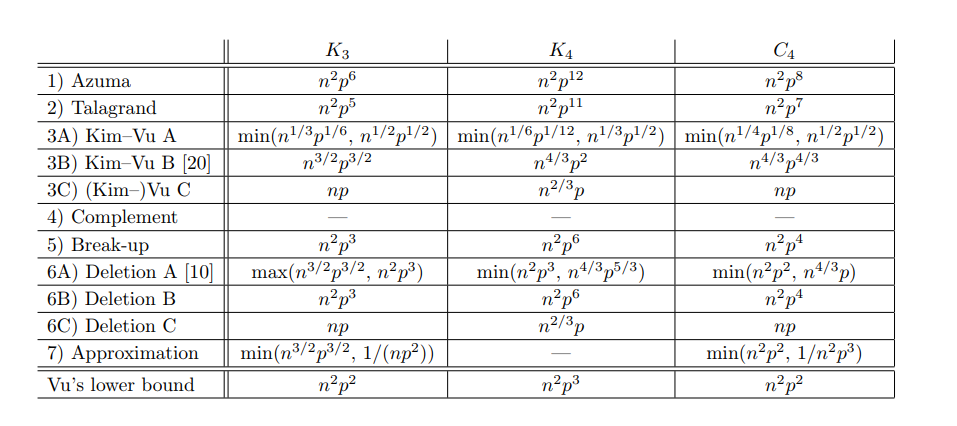
Refer to caption
Figure 1: [29] Exponents for upper tails in the small subgraphs problem

Although we are mainly dealing with $G(n,M)$ in this section, it is well known that $G(n,M)$ and $G(n,p)$ with $p=M/\binom{n}{2}$ behaves similarly when $n^{2}p\to\infty$. Applying the inequalities in (11) to $K_{3},K_{4},C_{4}$ respectively, we have that the exponents (ignoring constant) obtained from the Ricci curvature method are $n^{2}p^{5}$, $n^{2}p^{11}$ and $n^{2}p^{7}$ respectively. In this context, the concentration we obtained from Theorem 1 has the same strength as Talagrand inequality and slightly stronger than Azuma’s inequality.

4.3 Edge-Lipschitz functions on random hypergraphs

Let $\mathcal{H}\sim\mathcal{H}^{k}(n,M)$ be a random $k$-uniform hypergraph with $n$ vertices and $M$ edges. Let $H$ be a graph such that $V(H)$ is the set of all labeled $k$-uniform hypergraphs with $n$ vertices and $M$ edges. Moreover, two hypergraphs $\mathcal{H}_{1},\mathcal{H}_{2}\in V(H)$ are adjacent in $H$ if and only if there exist two distinct $k$-sets $h_{1},h_{2}$ such that $h_{1}\in E(\mathcal{H}_{1})\backslash E(\mathcal{H}_{2})$, $h_{2}\in E(\mathcal{H}_{2})\backslash E(\mathcal{H}_{1})$ and $\mathcal{H}_{1}-h_{1}=\mathcal{H}_{2}-h_{2}$. In other words, $\mathcal{H}_{1},\mathcal{H}_{2}$ are adjacent in $H$ if one can be obtained from the other by swapping a hyperedge with a non-hyperedge. It is easy to see that $H$ is a connected regular graph. Moreover, for every $\mathcal{H}\in V(H)$, $d_{H}(\mathcal{H})=M\left(\binom{n}{k}-M\right)$. Now define a random walk $m$ on $H$ as follows: Let $\mathcal{H}\in V(H)$. Define

$$m_{\mathcal{H}}(\mathcal{H}^{\prime})=\begin{cases}\frac{1}{M\left(\binom{n}{k}-M\right)+1}&\textrm{ if $\mathcal{H}^{\prime}\in\Gamma(\mathcal{H})$,}\\ 0&\textrm{ otherwise.}\end{cases}$$

By the same logic in Section 4.2, we can obtain a lower bound for the Ricci curvature of $H$, i.e., for all $\mathcal{H}_{1},\mathcal{H}_{2}\in V(H)$,

$$\kappa(\mathcal{H}_{1},\mathcal{H}_{2})\geq\frac{\binom{n}{k}}{M\left(\binom{n}{k}-M\right)+1}.$$

Similar to before, we can also apply Theorem 1 to obtain concentration results for the number of copies of fixed sub-hypergraphs in a uniformly random hypergraph on $n$ vertices and $M$ edges. The idea is similar to Section 4.2 and we leave the details to the readers.

4.4 Vertex-Lipschitz functions on random $d$-out(in)-regular graphs

Given a directed graph $G$ and a vertex $v$, we use $\delta^{+}(v)$ and $\delta^{-}(v)$ to denote the outdegree and indegree, respectively, of a vertex $v$. A $d$-out-regular graph $G$ is a directed graph in which $\delta^{+}(v)=d$ for every $v\in V(G)$. Similarly, a $d$-in-regular graph $G$ is a directed graph in which $\delta^{-}(v)=d$ for every $v\in V(G)$. Moreover, let $\Gamma^{+}(v)=\{u\in V(G):vu\in E(G)\}$, $\Gamma^{-}(v)=\{u\in V(G):uv\in E(G)\}$, $N^{+}(v)=\Gamma^{+}(v)\cup\{v\}$ and $N^{-}(v)=\Gamma^{-}(v)\cup\{v\}$.

Let $H$ be a graph such that $V(H)$ is the set of all labeled $d$-out-regular graphs on $n$ vertices. Two graphs $G_{1},G_{2}\in V(H)$ are adjacent in $H$ if and only if there exists some vertex $v\in V(G_{1})=V(G_{2})$ such that one can be obtained from the other by changing $\Gamma^{+}(v)$. It is not hard to see that $H$ is a connected graph with $diam(H)\leq n$. Moreover, it is also clear that if $G_{1},G_{2}$ are adjacent in $H$, there is a unique vertex $v$ such that one can be obtained from the other by changing $\Gamma^{+}(v)$.

Now define a random walk $m$ on $H$ as follows: let $G\in V(H)$ and define

$$m_{G}(G^{\prime})=\begin{cases}\frac{1}{n\left(\binom{n-1}{d}-1\right)+1}&\textrm{ if $G^{\prime}\in N^{+}(G)$,}\\ 0&\textrm{ otherwise}.\end{cases}$$

It’s easy to see that for a fixed $G$, $\sum_{G^{\prime}}m_{G}(G^{\prime})=1$.

Proposition 5.

Let $\nu$ be the unique invariant distribution of the random walk defined above. A random graph $G$ picked according to $\nu$, is equally likely to be one of the $d$-out-regular graphs on $n$ vertices.

Proof.

Observe that $H$ is not bipartite thus the random walk is ergodic. There are $\binom{n-1}{d}^{n}$ many $d$-out-regular graphs in total. Hence, it suffices to show that $\nu^{\prime}(G)=\binom{n-1}{d}^{-n}$ for every $G$ is an invariant distribution for the random walk. Indeed, for every fixed $G\in V(H)$,

$\displaystyle\displaystyle\sum_{G^{\prime}\in H}\nu^{\prime}(G^{\prime})m_{G^{\prime}}(G)$ $\displaystyle=\binom{n-1}{d}^{-n}\displaystyle\sum_{G^{\prime}\in H}m_{G^{\prime}}(G)$
$\displaystyle=\binom{n-1}{d}^{-n}\displaystyle\sum_{G^{\prime}\in H}m_{G}(G^{\prime})$
$\displaystyle=\binom{n-1}{d}^{-n}$
$\displaystyle=\nu^{\prime}(G).$

Since $\nu$ is the unique invariant distribution, it follows then that $\nu=\nu^{\prime}$. ∎

Lemma 6.

Let $H$ and the random walk $m$ be defined as above. Then

$$\kappa(G_{1},G_{2})\geq\frac{1}{n}$$

for all $G_{1},G_{2}\in V(H)$.

Proof.

Again, by Lemma 1, we can assume that $G_{1},G_{2}$ are neighbors in $H$. It then follows from definition that

$$\kappa(G_{1},G_{2})=1-W(m_{G_{1}},m_{G_{2}}).$$

Suppose $v$ is the unique vertex such that $G_{2}$ can be obtained from $G_{1}$ by changing $\Gamma^{+}(v)$. Consider the support of $m_{G_{1}}$. For each $G_{1}^{\prime}\in N(G_{1})$, we will match $G_{1}^{\prime}$ with a distinct graph $\phi(G_{1}^{\prime})\in N(G_{2})$. Again, let $\phi(G_{1})=G_{1}$ and $\phi(G_{2})=G_{2}$. For other neighbors $G_{1}^{\prime}$ of $G_{1}$, there are two possible cases:

Case $1$: $G_{1}-v=G_{1}^{\prime}-v$. Then it follows that $G_{1}^{\prime}-v=G_{2}-v$ and we let $\phi(G_{1}^{\prime})=G_{1}^{\prime}$.

Case $2$: $G_{1}-u=G_{1}^{\prime}-u$ for some $u\neq v$. In this case, we claim that for each $G_{1}^{\prime}$ such that $G_{1}-u=G_{1}^{\prime}-u$, there exists a unique $G_{2}^{\prime}=\phi(G_{1}^{\prime})$ such that $G_{2}^{\prime}-u=G_{2}-u$ and $G_{1}^{\prime}-v=G_{2}^{\prime}-v$. Indeed, let $G_{2}^{\prime}$ be obtained from $G_{2}$ by replacing the out-neighbors of $u$ in $G_{2}$ by the out-neighbors of $u$ in $G_{1}^{\prime}$. It’s not hard to see that $G_{2}^{\prime}-u=G_{2}-u$ and $G_{1}^{\prime}-v=G_{2}^{\prime}-v$.

Let us now define a coupling $A$ (not necessarily optimal) between $m_{G_{1}}$ and $m_{G_{2}}$. Define $A:V(H)\times V(H)\to\mathbb{R}$ as follows:

$$A(G_{1}^{\prime},G_{2}^{\prime})=\begin{cases}\frac{1}{n\left(\binom{n-1}{d}-1\right)+1}&\textrm{ if }G_{1}^{\prime}\in N(G_{1})\textrm{ and $G_{2}^{\prime}=\phi(G_{1}^{\prime})$,}\\ 0&\textrm{ otherwise. }\end{cases}$$ (12)

It is not hard to verify that $A$ is a coupling of $m_{G_{1}}$ and $m_{G_{2}}$. Now by definition,

$\displaystyle W(m_{G_{1}},m_{G_{2}})$ $\displaystyle\leq\displaystyle\sum_{G_{1}^{\prime},G_{2}^{\prime}}A(G_{1}^{\prime},G_{2}^{\prime})d(G_{1}^{\prime},G_{2}^{\prime})$
$\displaystyle\leq\displaystyle\sum_{u\neq v}\displaystyle\sum_{\begin{subarray}{c}G_{1}^{\prime}\in N(G_{1})\\ G_{1}^{\prime}-u=G_{1}-u\end{subarray}}A(G_{1}^{\prime},\phi(G_{1}^{\prime}))d(G_{1}^{\prime},\phi(G_{1}^{\prime}))$
$\displaystyle\leq(n-1)\left(\binom{n-1}{d}-1\right)\frac{1}{n\left(\binom{n-1}{d}-1\right)+1}$

It follows that

$$\kappa(G_{1},G_{2})=1-W(m_{G_{1}},m_{G_{2}})\geq\frac{\binom{n-1}{d}}{n\left(\binom{n-1}{d}-1\right)+1}\geq\frac{1}{n}.$$

This completes the proof of the lemma. ∎

Let $G$ be a uniformly random $d$-out-regular graph. A directed triangle is a cycle of length $3$ with vertices $u,v,w$ such that $uv,vw$ and $wu$ are all directed edges. Let $X_{n,d}:=X(G)$ be the random variable denoting the number of directed triangle in $G$. It is not hard to see that

$$E[X_{n,d}]\approx 2\binom{n}{3}\left(\frac{d}{n-1}\right)^{3}.$$

We will now use Theorem 1 to derive the concentration behavior of $X_{n,d}$. Note that $X_{n,d}$ is $(d^{2})$-Lipschitz. Hence by Theorem 1, we have that

$$\Pr\left(\left\lvert\frac{X_{n,d}}{d^{2}}-\frac{E[X_{n,d}]}{d^{2}}\right\rvert>\frac{t}{d^{2}}\right)\leq 2\exp{\left(-\frac{t^{2}\kappa}{5d^{4}}\right)}.$$

It follows that

$$\Pr\left(\left\lvert X_{n,d}-E[X_{n,d}]\right\rvert>t\right)\leq 2\exp{\left(-\frac{t^{2}\kappa}{5d^{4}}\right)}\leq 2\exp{\left(-\frac{t^{2}}{5nd^{4}}\right)}.$$

4.5 Lipschitz functions on random linear permutations

We will denote a linear permutation $\sigma$ by $\sigma=[a_{1}a_{2}\ldots a_{n}]$ such that $a_{i}\in[n]$ for all $i$ and $\sigma(i)=a_{i}$. A linear permutation on $[n]$ can be viewed as a sequence of $n$ distinct numbers from $[n]$. Thus, WLOG, $\{a_{1},a_{2},\ldots,a_{n}\}=[n]$. Given two permutations $\sigma_{1},\sigma_{2}$ where $\sigma_{1}=[a_{1}a_{2}\ldots a_{n}]$, we say $\sigma_{1}$ is $(i,j)$-alike to $\sigma_{2}$ if $\sigma_{2}$ can be obtained from $\sigma_{1}$ by moving the number $i$ to the position after the number $j$ in $\sigma_{1}$; moreover, $\sigma_{1}$ is $(i,0)$-alike to $\sigma_{2}$ if $\sigma_{2}$ can be obtained from $\sigma_{1}$ by moving the number $i$ to the first position of $\sigma_{1}$. For example, $\sigma_{1}=[12345]$ is $(2,4)$-alike to $\sigma_{2}=[13425]$ and is $(4,0)$-alike to $\sigma_{3}=[41235]$. Two distinct linear permutations $\sigma_{1},\sigma_{2}$ are insertion-alike if one is $(i,j)$-alike to the other for some $i\neq j$.

Let $H$ be the graph such that $V(H)$ is the set of all linear permutations of $[n]$ and two linear permutation $\sigma_{1},\sigma_{2}$ are adjacent in $H$ if and only if they are insertion-alike. Clearly $H$ is a connected graph with diameter at most $n$. Moreover, every vertex (which is a linear permutation) in $H$ has $(n-1)^{2}$ neighbors in $H$.

Now define a random walk $m_{\alpha}$ on $H$ as follows: let $\sigma\in V(H)$ and define

$$m_{\sigma}(\sigma^{\prime})=\begin{cases}\frac{1}{(n-1)^{2}+1}&\textrm{ if $\sigma=\sigma^{\prime}$ or $\sigma$ is insertion-alike to $\sigma^{\prime}$,}\\ 0&\textrm{ otherwise}.\end{cases}$$

It’s not hard to see that for a fixed $\sigma$, $\sum_{\sigma^{\prime}}m_{\sigma}(\sigma^{\prime})=1$. Moreover, $m_{\sigma}(\sigma^{\prime})=m_{\sigma^{\prime}}(\sigma)$ for every pair of $\sigma,\sigma^{\prime}$.

Proposition 6.

Let $\nu$ be the unique invariant distribution of the random walk defined above. A random permutations $\sigma$ picked according to $\nu$, is equally likely to be one of the $n!$ permutations.

Proof.

Observe that $H$ is not bipartite thus the random walk is ergodic. There are $n!$ permutations in total. Hence, it suffices to show that $\nu^{\prime}(\sigma)=(n!)^{-1}$ for every $\sigma$ is an invariant distribution for the random walk.

$\displaystyle\displaystyle\sum_{\sigma^{\prime}\in H}\nu^{\prime}(\sigma^{\prime})m_{\sigma^{\prime}}(\sigma)$ $\displaystyle=\frac{1}{n!}\displaystyle\sum_{\sigma^{\prime}\in V(H)}m_{\sigma^{\prime}}(\sigma)$
$\displaystyle=\frac{1}{n!}\displaystyle\sum_{\sigma^{\prime}\in V(H)}m_{\sigma}(\sigma^{\prime})$
$\displaystyle=\frac{1}{n!}$
$\displaystyle=\nu^{\prime}(\sigma).$

Since $\nu$ is the unique invariant distribution, it follows then that $\nu=\nu^{\prime}$. ∎

Lemma 7.

Let $H$ and the random walk $m$ be defined as above. If $\sigma_{1},\sigma_{2}\in V(H)$ are neighbors in $H$, then $\kappa(\sigma_{1},\sigma_{2})\geq\frac{1}{n}$.

Proof.

WLOG, suppose that $\sigma_{1}$ is $(i,j)$-alike to $\sigma_{2}$ (with $\sigma_{2}\neq\sigma_{1}$). Consider the support of $m_{\sigma_{1}}$. For each $\sigma_{1}^{\prime}\in N(\sigma_{1})$, we will match $\sigma_{1}^{\prime}$ with a distinct permutation $\phi(\sigma_{1}^{\prime})\in N(\sigma_{2})$. First let $\phi(\sigma_{1})=\sigma_{1}$ and $\phi(\sigma_{2})=\sigma_{2}$. For other neighbors $\sigma_{1}^{\prime}$ of $\sigma_{1}$, there are two cases:

Case $1$: $\sigma_{1}$ is $(i,k)$-alike to $\sigma_{1}^{\prime}$ where $k\neq j$. Then it follows that $\sigma_{1}^{\prime}$ is also $(i,j)$-alike to $\sigma_{2}$ and we let $\phi(\sigma_{1}^{\prime})=\sigma_{1}^{\prime}$.

Case $2$: $\sigma_{1}$ is $(i^{\prime},j^{\prime})$-alike to $\sigma_{1}^{\prime}$ where $i^{\prime}\neq i$ and $\sigma_{1}$ is not $(i,k)$-alike to $\sigma_{1}^{\prime}$ for any $k$. In this case, let $\sigma_{2}^{\prime}$ be the permutation such that $\sigma_{2}$ is $(i^{\prime},j^{\prime})$-alike to $\sigma_{2}^{\prime}$. It follows easily that $\sigma_{1}^{\prime}$ is also $(i,j)$-alike to $\sigma_{2}^{\prime}$. We then define $\phi(\sigma_{1}^{\prime})=\sigma_{2}^{\prime}$.

Let us now define a coupling $A$ (not necessarily optimal) between $m_{\sigma_{1}}$ and $m_{\sigma_{2}}$. Define $A:V(H)\times V(H)\to\mathbb{R}$ as follows:

$$A(\sigma_{1}^{\prime},\sigma_{2}^{\prime})=\begin{cases}\frac{1}{(n-1)^{2}+1}&\textrm{ if }\sigma_{1}^{\prime}\in N(\sigma_{1})\textrm{ and $\sigma_{2}^{\prime}=\phi(\sigma_{1}^{\prime})$,}\\ 0&\textrm{ otherwise. }\end{cases}$$ (13)

It is not hard to verify that $A$ is a coupling of $m_{\sigma_{1}}$ and $m_{\sigma_{2}}$. Now by definition,

$\displaystyle W(m_{\sigma_{1}},m_{\sigma_{2}})$ $\displaystyle\leq\displaystyle\sum_{\sigma_{1}^{\prime},\sigma_{2}^{\prime}}A(\sigma_{1}^{\prime},\sigma_{2}^{\prime})d(\sigma_{1}^{\prime},\sigma_{2}^{\prime})$
$\displaystyle\leq\displaystyle\sum_{\sigma^{\prime}\in N(\sigma_{1})}A(\sigma_{1}^{\prime},\phi(\sigma_{1}^{\prime}))d(\sigma_{1}^{\prime},\phi(\sigma_{1}^{\prime}))$
$\displaystyle\leq 1-\frac{n}{(n-1)^{2}+1}.$

It follows that

$$\kappa(\sigma_{1},\sigma_{2})=1-W(m_{\sigma_{1}},m_{\sigma_{2}})\geq\frac{n}{(n-1)^{2}+1}\geq\frac{1}{n}.$$

This completes the proof of the lemma. ∎

Now we give an example of concentration results on the space of random linear permutations. In particular, we discuss the number of occurrences of certain patterns in random permutations. Denote the set of length $n$ linear permutations by $\mathcal{S}_{n}$. Given a permutation pattern $\tau\in\mathcal{S}_{k}$, we say that a permutation $\pi=[\pi_{1}\ldots\pi_{n}]\in\mathcal{S}_{n}$ contains the pattern $\tau$ if there exists $1\leq i_{1}<i_{2}<\ldots<i_{k}\leq n$ such that the $\pi_{i_{s}}<\pi_{i_{t}}$ if and only if $\tau_{s}<\tau_{t}$ for every pair $s,t$. Each such subsequence in $\pi$ is called an occurrence of the pattern $\tau$. Let $\tau$ be a random permutation in $\mathcal{S}_{n}$ and let the random variable $X_{\tau,n}:=X_{\tau}(\pi)$ be the number of copies of $\tau$ in $\pi$. We consider asymptotics as $n\to\infty$ for (one or several) fixed $\tau$.

The (joint) distribution of the $X_{\tau,n}$ has been investigated in a series of paper [5, 6, 27]. In particular, Bona [5] showed that for every $\tau\in\mathcal{S}_{k}$, as $n\to\infty$,

$$\frac{X_{\tau,n}-E[X_{\tau,n}]}{n^{k-\frac{1}{2}}}\to N(0,Z_{\tau})$$ (14)

for some $Z_{\tau}>0$. Janson, Nakamura and Zeilberger [27] showed that the above holds jointly for any finite family of patterns $\tau$.

Note that as a consequence of the convergence in (14), we obtain the following concentration inequality:

$$\Pr\left(\left\lvert X_{\tau,n}-E[X_{\tau,n}]\right\rvert>t\right)\leq 2\exp\left(-\frac{t^{2}}{2n^{2k-1}Z_{\tau}}\right)$$ (15)

which is sharp up to a polynomial factor.

On the other hand, consider the graph $H$ defined at the beginning of this subsection, where $V(H)$ is the set of all linear permutations of $[n]$. It is not hard to see that the function $X_{\tau,n}:V(H)\to\mathbb{Z}$ is $\binom{n-1}{k-1}$-Lipschitz. It follows by Theorem 1 that

$\displaystyle\Pr\left(\left\lvert\frac{X_{\tau,n}}{\binom{n-1}{k-1}}-\frac{E[X_{\tau,n}]}{\binom{n-1}{k-1}}\right\rvert>\frac{t}{\binom{n-1}{k-1}}\right)$ $\displaystyle\leq 2\exp\left(-\frac{t^{2}\kappa}{5\binom{n-1}{k-1}^{2}}\right)$
$\displaystyle\leq 2\exp\left(-\frac{t^{2}}{C_{k}n^{2k-1}}\right)$

for some $C_{k}>0$. Hence the concentration result in Theorem 1 is in fact asymptotically optimal in the case of counting occurrences of patterns in random permutations.

Remark 6.

Similar Ricci curvature and concentration results can be obtained for the space of cyclic permutations as well.

Remark 7.

Another possible way to geometrize the space of linear permutations is the random transposition model (see, e.g., [24]) as follows: let $V(H)=\mathcal{S}_{n}$ and two permutations $\sigma_{1},\sigma_{2}\in V(H)$ are adjacent in $H$ if $\sigma_{2}=\tau\circ\sigma_{1}$ for some transposition $\tau$. Define a random walk $m$ on $H$ by

$$m_{\sigma}(\sigma^{\prime})=\begin{cases}\frac{2}{n(n-1)}&\textrm{ if $\sigma$ and $\sigma^{\prime}$ are adjacent in $H$,}\\ 0&\textrm{ otherwise}.\end{cases}$$

The invariant distribution is the uniform measure on $\mathcal{S}_{n}$. The Ricci curvature of this graph is $\Theta(n^{-2})$, as observed by Gozlan et al [25].

References

  • [1] R. Adamczak and P. Wolff, Concentration inequalities for non-Lipschitz functions with bounded derivatives of higher order, Probab. Theory Related Fields 162(3) (2015), 531–586.
  • [2] N. Alon and J. H. Spencer, The Probabilistic Method, Wiley-Interscience, third edition, 2008.
  • [3] K. Azuma, Weighted sum of certain independent random variables, Tohoku Math. J. 19 (3) (1967) 357-–367.
  • [4] D. Bakry and M. Emery, Diffusions hypercontractives, Séminaire de probabilités, XIX, 1983/84, 177-–206, Lecture Notes in Math. 1123, Springer, Berlin, 1985.
  • [5] Miklós Bóna, The copies of any permutation pattern are asymptotically normal, arXiv:0712.2792 (2007).
  • [6] Miklós Bóna, On three different notions of monotone subsequences, Permutation Patterns, 89-–114, London Math. Soc. Lecture Note Ser., 376, Cambridge Univ. Press, Cambridge, 2010.
  • [7] S. Chatterjee, The missing log in large deviations for triangle counts, Random Structures Algorithms, 40(4) (2012), 437–451.
  • [8] F. Chung, A. Grigor’yan and S.-T. Yau, Upper bounds for eigenvalues of the discrete and continuous Laplace operators, Adv. Math. 117 (1996), 165-–178.
  • [9] F. Chung and L. Lu, Concentration inequalities and martingale inequalities: a survey, Internet Math., 3(1) (2006) 79-–127.
  • [10] F. Chung and S.-T. Yau, A Harnack inequality for homogeneous graphs and subgraphs, Comm. Anal. Geom. 2 (1994), 627–-640, also in Turkish J. Math. 19 (1995), 273-–290.
  • [11] F. Chung and S.-T. Yau, Eigenvalues of graphs and Sobolev inequalities, Combin. Probab. Comput. 4 (1995), 11-–25.
  • [12] F. Chung and S.-T. Yau, Logarithmic Harnack inequalities, Math. Res. Lett. 3 (1996), 793-–812.
  • [13] F. Chung and S.-T. Yau, A combinatorial trace formula, Tsing Hua lectures on geometry & analysis (Hsinchu, 1990–1991), 107–-116, Int. Press, Cambridge, MA, 1997.
  • [14] F. Chung, A. Grigor’yan and S.-T. Yau, Eigenvalues and diameters for manifolds and graphs, Tsing Hua lectures on geometry & analysis (Hsinchu, 1990–1991), 79–105, Int. Press, Cambridge, MA, 1997.
  • [15] F. Chung and S.-T. Yau, Coverings, heat kernels and spanning trees, Electron. J. Combin. 6 (1999), Research Paper 12, 21pp.
  • [16] F. Chung and S.-T. Yau, Spanning trees in subgraphs of lattices, Contemp. Math. 245, 201–-219, Amer. Math. Soc., Providence, R.I., 1999.
  • [17] F. Chung and S.-T. Yau, A Harnack inequality for Dirichlet eigenvalues, J. Graph Theory 34 (2000), 247–-257.
  • [18] F. Chung, A. Grigor’yan and S.-T. Yau, Higher eigenvalues and isoperimetric inequalities on Riemannian manifolds and graphs, Comm. Anal. Geom. 8 (2000), 969–-1026.
  • [19] F. Chung and S.-T. Yau, Discrete Green’s functions, J. Combin. Theory Ser. A 91 (2000), 191-–214.
  • [20] B. DeMarco and J. Kahn, Upper tails for triangles, Random Structures Algorithms, 40(4) (2012), 452–459.
  • [21] B. DeMarco and J. Kahn, Tight upper tail bounds for cliques, Random Structures Algorithms 41(4) (2012), 469–487.
  • [22] H. Djellout, A. Guillin, L. Wu, Transportation cost-information inequalities and applications to random dynamical systems and diffusions, Ann. Probab. 32 (3B) (2004) 2702-–2732.
  • [23] M. Erbar, J. Maas, Ricci curvature of finite Markov chains via convexity of the entropy. Arch. Ratnl Mech. Anal., 206, (2012) 997–1038.
  • [24] M. Erbar, J. Maas, and P. Tetali, Discrete Ricci Curvature bounds for Bernoulli-Laplace and Random Transposition models. Annales de la faculté des sciences de Toulouse Mathématiques, 24(4) (2016) 781–800. 2015.
  • [25] N. Gozlan, J. Melbourne, W. Perkins, C. Roberto, P-M. Samson, and P. Tetali. Working Group in New directions in mass transport: discrete versus continuous. AIM SQuaRE report, October, 2013.
  • [26] W. Hoeffding, Probability inequalities for sums of bounded random variables, J. Amer. Statist. Assoc. 58 (1963) 13–-30.
  • [27] S. Janson, B. Nakamura, and D. Zeilberger, On the asymptotic statistics of the number of occurrences of multiple permutation patterns, Journal of Combinatorics, 6 (2015) 117-–143.
  • [28] S. Janson, K. Oleszkiewicz, and A. Ruciński, Upper tails for subgraph counts in random graphs, Israel J. Math. 142 (2004), 61–92.
  • [29] S. Janson and A. Ruciński, The infamous upper tail, Random Structures and Algorithms 20 (2002), 317–342.
  • [30] A. Joulin, A new Poisson-type deviation inequality for Markov jump processes with positive Wasserstein curvature, Bernoulli 15 (2009), 532–-549.
  • [31] A. Joulin and Y. Ollivier, Curvature, concentration and error estimates for Markov chain Monte Carlo, Ann. Probab. 38(6) (2010), 2418–2442.
  • [32] Y. Lin, L. Lu, S. T. Yau, Ricci curvature of graphs, Tohoku Math. J. 63 (2011) 605–627.
  • [33] J. Lott and C. Villani, Ricci curvature for metric-measure spaces via optimal transport. Ann. of Math. (2), 169(3) (2009), 903–991.
  • [34] Y. Lin and S.-T. Yau, Ricci curvature and eigenvalue estimate on locally finite graphs, Mathematical Research Letters 17 (2010), 345-–358.
  • [35] J. Maas, Gradient flows of the entropy for finite Markov chains, J. Funct. Anal., 261 (2011), 2250–2292.
  • [36] A. Mielke, Geodesic convexity of the relative entropy in reversible Markov chains, Calc. Var. Partial Differential Equations, 48 (2013), 1-–31.
  • [37] M.D. Sammer. Aspects of mass transportation in discrete concentration inequalities. PhD thesis, Georgia Institute of Technology, 2005.
  • [38] K.-Th. Sturm. On the geometry of metric measure spaces. I and II. Acta Math., 196(1) (2006), 65–177.
  • [39] Y. Ollivier, Ricci curvature of Markov chains on metric spaces, J. Funct. Anal. 256 (2009), 810–-864.