(1a) & m= number of snapshots taken (1b) T h e D M D a l g o r i t h m w a s o r i g i n a l l y d e s i g n e d t o c o l l e c t d a t a a t r e g u l a r l y s p a c e d i n t e r v a l s o f t i m e . H o w e v e r , n e w i n n o v a t i o n s a l l o w f o r b o t h s p a r s e s p a t i a l Brunton et al. (2015 a n d t e m p o r a l Tu et al. (2014a c o l l e c t i o n o f d a t a a s w e l l a s i r r e g u l a r l y s p a c e d c o l l e c t i o n t i m e s Askham and Kutz (2018 . I n d e e d , T u et al. Tu et al. (2014b p r o v i d e s a h i g h l y i n t u i t i v e d e f i n i t i o n o f t h e D M D m e t h o d a n d a l g o r i t h m . & ( 1 c )
𝐃𝐞𝐟𝐢𝐧𝐢𝐭𝐢𝐨𝐧 : 𝐃𝐲𝐧𝐚𝐦𝐢𝐜𝐌𝐨𝐝𝐞𝐃𝐞𝐜𝐨𝐦𝐩𝐨𝐬𝐢𝐭𝐢𝐨𝐧 ( T u et al. 2014 Tu et al. (2014b ) : S u p p o s e w e h a v e a d y n a m i c a l s y s t e m a n d t w o s e t s o f d a t a X = [x 1 x 2 ⋯x m-1 ] (2a) (2b) X ’ = [ x ’ 1 x ’ 2 ⋯ x ’ m-1 ] (2c) so that 𝐱 k ′ = 𝐅 ( 𝐱 k ) where 𝐅 is the flow map corresponding to the evolution of our dynamical system for time Δ t . DMD computes the leading eigendecomposition of the best-fit linear operator 𝐀 relating the data 𝐗 ′ ≈ 𝐀𝐗 :
The DMD modes, also called dynamic modes, are the eigenvectors of 𝐀 , and each DMD mode corresponds to a particular eigenvalue of 𝐀 . (3)
In the DMD architecture, we typically consider data collected from a dynamical system
where 𝐱 ( t ) ∈ ℝ n is a vector representing the state of our dynamical system at time t , 𝝁 contains parameters of the system, and 𝐟 ( ⋅ ) represents the dynamics. For instance, the vector 𝐱 denotes the
power grid state after numerical discretization while 𝝁 is a parametrization of the system.
The state 𝐱 is typically quite large, having dimension n ≫ 1 .
Measurements of the system
are collected at times t k from k = 1 , 2 , ⋯ , m for a total of m measurement times.
The measurements are typically the state of the power grid, so that 𝐲 k = 𝐱 k , however, the DMD architecture
allows for a more nuianced viewpoint of observables. This is beyond the scope of the current work, but such ideas
are related to Koopman theory Mezic (2013 Kutz et al. (2016 .
The DMD framework takes an equation-free perspective where the original, nonlinear dynamics (e.g. network level power grid dynamics) may be unknown. Thus data measurements of the system alone are used to approximate the dynamics and predict the future state. Measurements can also be made on functions of the state space, resulting in the so-called Koopman operator Mezic (2013 Kutz et al. (2016 , which has been used previously to study power grid dynamics Susuki et al. (2009 2011 Susuki and Mezic (2011 2012 Susuki and Mezić (2014 . The DMD procedure constructs the proxy, approximate locally linear dynamical system
with initial condition 𝐱 ( 0 ) whose well-known solution is
x ( t ) = ∑ = k 1 n ϕ k exp ( ω k t ) b k = Φ exp ( Ω t ) b (7)
where ϕ k and ω k are the eigenvectors and eigenvalues of the matrix 𝐀 , and the coefficients b k are the coordinates of 𝐱 ( 0 ) in the eigenvector basis.
The DMD algorithm produces a low-rank eigen-decomposition of the matrix 𝐀 that optimally fits the measured trajectory 𝐱 k for k = 1 , 2 , ⋯ , m in a least square sense so that
is minimized across all points for k = 1 , 2 , ⋯ , m − 1 .
The optimality of the approximation holds only over the sampling window where 𝐀 is constructed, and the approximate solution can be used to not only make future state predictions, but also to derive dynamic modes critical for diagnostics. Indeed, in much of the literature where DMD is applied, it is primarily used as a diagnostic tool. This is much like POD analysis where the POD modes are also primarily used for diagnostic purposes. Thus the DMD algorithm can be thought of as a modification of the SVD architecture which attempts to account for dynamic activity of the data. The eigendecomposition of the low rank space found from SVD enforces a Fourier mode time expansion which allows one to then make spatio-temporal correlations with the sampled data.
II.2 Compressive Sensing and Sparse Sensors
Although the gappy POD method Everson and Sirovich (1995 Willcox (2006 Yildirim et al. (2009 Chaturantabut and Sorensen (2010 Sargsyan et al. (2015 Bright et al. (2013 Brunton et al. (2014 Proctor et al. (2014 Kramer et al. (2015 ℓ 1
Consider a high-dimensional measurement vector of the power grid system ∈ x R n Ψ
Here, sparsity means that x Ψ a K sparsity means that there are K compressible .
Consider a sparse measurement of the power grid system ∈ y R p ≪ p n
where Φ x y 9 10
We may then solve for the sparsest solution a 11 ℓ 0 a | a | 0 | a | 1 Candès et al. (59 Donoho (2006
= arg min | ^ a | 1 such that Φ Ψ ^ a y .
There are other algorithms that result in sparse solution vectors, such as orthogonal matching pursuit Tropp and Gilbert (2007
This procedure, known as compressive sensing , is a recent development that has had widespread success across a range of problems. There are technical issues that must be addressed. For example, the number of measurements p y K log ( / n K ) K a Ψ Candès (2006 Candès et al. (2006 Baraniuk (2007 Φ incoherent with respect to the sparse basis Ψ Φ Ψ Candès and Tao (2006
Typically a generic basis such as Fourier or wavelets is used in conjunction with sparse measurements consisting of random projections of the state. However, in many engineering applications, it is unclear how random projections may be obtained without first starting with a dense measurement of the state. In this work, we constrain the measurements to be point measurements of the state, so that Φ
II.3 Combining Methodologies
Figure 2 Ψ Ψ
III Power Systems Model
Table 1: Areas for the IEEE 118 Bus System
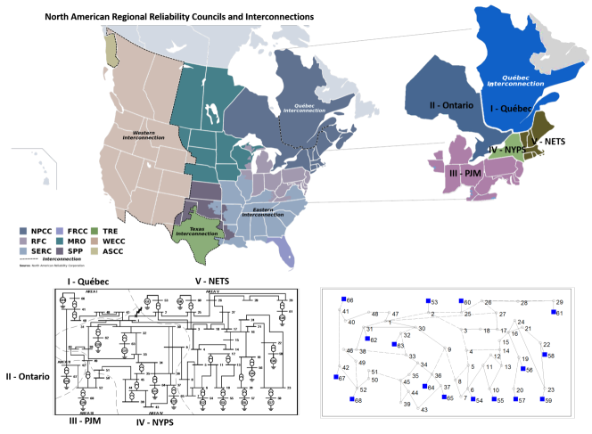
To demonstrate the application of the proposed methodology on complex dynamical systems, we study the voltage profile of an IEEE test system model of a power system under disturbances. The IEEE test system is comprised of a 68-Bus, 16-machine, 5-Area System widely know in the power system literature. The IEEE 16-machine, 68-Bus test system is a reduced order equivalent of the interconnected New England test system (NETS) and New York power system (NYPS), with five geographical regions out of which NETS and NYPS are represented by a group of generators. The power imported from each of the three other neighboring areas (Quebec, Ontario and PJM) are approximated by equivalent generator models as shown in Figure 2. The NETS is represented by nine generators G1 to G9 and comprises the power system of the states of Maine, New Hampshire, Vermont, Massachuset, Connecticut and Rhode Island. The NYPS corresponds to power system of New York State and it is modeled by four generators G10 to G13. Generators G14 to G16 corresponds to the I-Quebec, II- Ontario and III-PJM regions.
Figure 3: Voltage profile of 68 buses at different regimes. After t=1 s there is a stable state, from t = 1 to t=1.01 the fault is applied (drop of voltage), and after t=1.01 the fault is cleared and the transient measurement is presented. Figure 4: DMD modes representation of Regime 5 with threshold of 80% of energy. The Mode 1 represents an exponential component with low damping, and higher values in buses close to the fault. Modes 2 and 3 represents an oscillatory mode with ? = 0.224 Hz and =-0.127.
The bus data, line data, and detailed generator data of IEEE 16-machine 68-Bus test system are given in Ref. Rogers (2012
In order to test the performance of the proposed methodology, 16 disturbances were simulated in the closest bus to the generator, producing 16 distinct regimes. The disturbances, a three-phase fault at a respective bus, were introduced after one second of steady state operation and cleared after 0.1 seconds. Since the phenomenon of interest after the disruption are low frequency oscillations between 0.1 to 2 Hz, a time interval of 6 seconds is used to analyze the behavior of the system after fault clearance. The 6 second time window is sufficiently long so that at least a half cycle of the slowest oscillation can be captured. Typical voltage profiles of 68 buses for most representative regimes are shown in Fig. 3.
The voltage of 68 buses were sample at a rate of 100 Hz by every regime. We then consider the possibility of using only 10, 15, 20 and 30 buses for the identification, classification and reconstruction of the dynamic regime. Sensor placement algorithms are described in the next section.
Figure 5: POD modes representation of Regime 5 with threshold of 80% of energy. The Modes 1, 2 and 3 represents irregular oscillatory components whithin higher values in buses close to the fault.Figure 6: Graph of sparse sensor placement on IEEE 16-machine 68-bus test system at different thresholds of energy (80%, 90%, 95% and 99%) for 10 and 20 sensors. The blue square represents the generators location. The red dots indicate the common sensor between thersholds energy and color circles shows independent sensors at every thresholdFigure 7: Accuracy of sensor placement for the library at 80% of energy at different time intervals and number of sensors considering a) Euclidean norm and b) Random sensor placement. There are considered a window of t=[0.1, 0.2, 0.4, 0.8, 1.4, 2.0, 3.0, 4.0] s. A 100 trials of random sensor placement are considered and the results are presented by boxplot in b) RND.Figure 8: Accuracy of sensor placement for the library at 99% of energy at different time intervals and number of sensors considering a) Euclidean norm and b) Random sensor placement. There are considered a window of t=[0.1, 0.2, 0.4, 0.8, 1.4, 2.0, 3.0, 4.0] s. A 100 trials of random sensor placement are considered and the results are presented by boxplot in b) RNDFigure 9: Voltage profile reconstruction of Regime 4 at t=1.54 s using 15 sensors and library of 80% of energy. The upper image shows a graph of IEEE test system with voltage profiles values represented though circle?s diameter and colorbar.The middle images represents voltage profiles values as a colored bars for true values and reconstruction values. Finally the lower figure shows the difference between true values and reconstruction values.Figure 10: Relative error for full voltage profile recontruction of all regimes at t=1.54 s using 15 and 20 sensors and library of 80% of energy.
IV Power Systems Networks Dynamics
The power system network dynamics are evaluated in two stages. During the first stage, a library of the dominant DMD modes all are extracted in order to determine a sensor placement. In the sparse measurement stage, the limited measurements are used to analyze, identify, classify and reconstruct the full voltages profiles of the power system.
IV.1 Library Learning
The 68-voltage measurements of every regime are analyzed by the DMD method to get a low dimensional representation of the data. DMD is used to construct a library of dominant DMD modes, which are the library elements that encode the low-rank dynamics of the power system for a specific regime or fault location.
DMD Regimes
Threshold
1
2
3
4
5 6
7
8
9
10
11
12
13
14
15
16
Library
elements
80%
2
3
2
2
3 3
2
3
2
4
2
2
4
2
2
2
40
90%
4
4
4
3
4 4
3
5
3
6
4
4
5
3
3
3
62
99%
10
11
11
8
9 11
10
11
8
12
10
11
11
8
6
8
155
POD Regimes
Threshold
1
2
3
4
5 6
7
8
9
10
11
12
13
14
15
16
Library
elements
80%
2
3
2
2
3 3
2
3
2
4
2
2
4
2
2
2
40
90%
4
4
4
3
4 4
3
5
3
6
4
4
5
3
3
3
62
99%
10
11
11
8
9 11
10
11
8
12
10
11
11
8
6
8
155
Table 2: Number of modes for every regime using DMD method and POD method for a threshold 80%, 90% and 99% of energy.
The number of DMD modes choosen to be part of library are limited to those modes that captures a prescribed percentage of energy (or observed variance), based on singular values from the SVD computed during the DMD procedure. The full state voltage profiles are low-rank so that the dynamics of the power system can be represented by a sparse number of modes. These modes are called the dominant modes. Table 1 shows the number of DMD modes selected to represent every regime according to the energy threshold of 80%, 90% and 99%. A comparison of the low dimensional representation between the DMD method and the POD modes is also presented in Table I.
Noticed that even when the number of modes for both methods are the same, their representation and meaning for the power network are different as it can be seen in Fig. 4 and Fig. 5.
IV.2 Sparse Sensor Placement for Classification
There are several ways to measure the importance of every sensor (or node) to the global behavior of the power system. A straightforward way is to measure the Euclidean norm between elements of library to rank every sensor. These projection onto the library elements give us an average of the importance of every sensor in the different regimes. The sensors can then be ordered from highest to lowest in the Euclidean norm, thus informing one of the number of sensors needed. The Fig. 6 shows a graph of sparse sensor placement on IEEE test system at different threshold of energy for the cases of 10 and 20 sensors.
Once the sparse sensor placement is defined, compressive sensing is used to identify, classify and reconstruct the full voltage profile of power system.
The identification and classification of every regime using a specific number of sensor are evaluating using the principles of compressive sensing outlined previously. The main assumption of compressed sensing in this context is that given measurement vector = y Φ Ψ a a y min ‖ a ‖ 1 = y Φ Ψ a a a y a
In general, better accuracy is achieved for the sparse sensor placement algorithm using the Euclidean norm versus random sensor placement. Also when the sampling window length of t
IV.3 Full State Reconstrution
The full voltage profile reconstruction can be easily achieved once the classification task is accomplished. The procedure consists in projecting the data measurements onto the identified dominant modes of the library for the given regime found from classification.
The full sate reconstruction is considered using a window length of 1.4 seconds for the identification of the regime and 15 and 20 sparse sensors placed using the library with 80% energy variance threshold. An example of the full voltage profile reconstruction is shown in Fig. 9. This reconstruction corresponds to the worst case of all regimes and the values of the difference between the true values and reconstruction values are located in the buses close to the fault. Even when this values exist, they are meaningless.
The relative error of full voltage profile reconstruction of all regimes at a specific snapshot using 15 and 20 sensors and library of 80% variance is displayed in Fig. 10. Noticed that higher values of relative error for 15 sensors belongs to R4, R8, R14 and R16, which suggests that four modes could not easily be correctly identified. However, the values of relative error for most of buses of these regimes remain at low levels. These results are improved when we use 20 sensors instead of 15 sensors. In this case, there are only two regimes with errors, R14 an R16. This results shown in Fig. 10 agrees with the accuracy results of Fig. 7.
V Conclusions
This paper proposes a data-driven framework for the analysis and visualization of power system disturbances. The approach is based on a semi-distributed algorithm that allows the computation of energy-based metrics from extracted consensus components. Specifically, we have further developed the DMD algorithm for characterizing the dynamics of disturbances in power grid networks and monitoring wide-area power grid networks from sparse measurement data.
Our proposed data-driven strategy, which is based on energy metrics, can be used for the analysis of major disturbances in the network. The approach is tested and validated using time domain simulations in the IEEE 118 bus system under various disturbance scenarios and under different sparse observations of the system. In addition to state reconstruction, the minimal number of sensors required for monitoring disturbances can be evaluated. Visualization techniques are developed in order to aid in the analysis and characterization of the system after disturbance.
With the emergence of advanced wide-area monitoring of power grid systems, it is important to develop data-driven methods that can continuously assess the power system health and performance. Central to such monitoring schemes are intelligent sensing methods, signal processing and communication technologies to make optimal use of measured wide-area data. We propose a new methodology for converting sparse, real-time measurements of a power grid into useful information that can be used to reconstruct the entire state space and produce short-time forecasts. The utility of such algorithms are central to timely detection and display of adverse conditions in the power grid. We have shown that the recently developed dynamic mode decomposition (DMD) is a promising data-driven method that allows for full state-space reconstruction and forecasting with limited measurements of the power grid system, thus enabling real-time monitoring capabilities.
Acknowledgements
JJR acknowledges support from National Council for Science and Technology of Mexico (CONACyT) under the grant No. 290733 and Cinvestav IPN. JNK acknowledges support from the U.S. Air Force Office of Scientific Research (FA9550-19-1-0011).
References
Messina and Messina [2015]
A. R. Messina and
A. R. Messina,
Wide-area monitoring of interconnected power systems
(The Institution of Engineering and Technology,
2015).
Kezunovic et al. [2013]
M. Kezunovic,
L. Xie, and
S. Grijalva, in
Bulk Power System Dynamics and Control-IX
Optimization, Security and Control of the Emerging Power Grid (IREP), 2013
IREP Symposium (IEEE, 2013), pp.
1–9.
Barocio et al. [2013]
E. Barocio,
B. C. Pal,
D. Fabozzi, and
N. F. Thornhill, in
Bulk Power System Dynamics and Control-IX
Optimization, Security and Control of the Emerging Power Grid (IREP), 2013
IREP Symposium (IEEE, 2013), pp.
1–10.
Susuki et al. [2009]
Y. Susuki,
I. Mezic, and
T. Hikihara, in
2009 American Control Conference
(IEEE, 2009), pp.
3446–3451.
Susuki et al. [2011]
Y. Susuki,
I. Mezić,
and T. Hikihara,
Journal of nonlinear science
21 , 403 (2011).
Susuki and Mezic [2011]
Y. Susuki and
I. Mezic,
IEEE Transactions on Power Systems
26 , 1894 (2011).
Susuki and Mezic [2012]
Y. Susuki and
I. Mezic,
IEEE Transactions on Power Systems
27 , 1182 (2012).
Susuki and Mezić [2014]
Y. Susuki and
I. Mezić,
IEEE Transactions on Power Systems
29 , 899 (2014).
Li et al. [2010]
W. Li,
J. Tang,
J. Ma, and
Y. Liu, IEEE
Transactions on Smart Grid 1 ,
253 (2010).
Mei et al. [2008]
K. Mei,
S. M. Rovnyak,
and C.-M. Ong,
IEEE Transactions on Power Systems
23 , 673 (2008).
Bhui and Senroy [2016]
P. Bhui and
N. Senroy,
IEEE Transactions on Power Systems
31 , 581 (2016).
Shahraeini et al. [2011]
M. Shahraeini,
M. H. Javidi,
and M. S.
Ghazizadeh, IEEE Transactions on Smart Grid
2 , 206 (2011).
Wang et al. [2015]
Y. Wang,
P. Yemula, and
A. Bose,
IEEE Transactions on Smart Grid
6 , 885 (2015).
Ning et al. [2013]
J. Ning,
X. Pan, and
V. Venkatasubramanian,
IEEE Transactions on Power Systems
28 , 1960 (2013).
Khalid and Peng [2015]
H. M. Khalid and
J. C.-H. Peng,
IEEE Transactions on Power Systems
30 , 680 (2015).
Nabavi et al. [2015]
S. Nabavi,
J. Zhang, and
A. Chakrabortty,
IEEE Transactions on Smart Grid
6 , 2529 (2015).
Eriksson and Soder [2011]
R. Eriksson and
L. Soder,
IEEE Transactions on Power Delivery
26 , 988 (2011).
Liu et al. [2015]
H. Liu,
L. Zhu,
Z. Pan,
F. Bai,
Y. Liu,
Y. Liu,
M. Patel,
E. Farantatos,
and N. Bhatt
(2015).
Pearson [1901]
K. Pearson,
Philosophical Magazine 2 ,
559 (1901).
Hotelling [1933a]
H. Hotelling,
24 , 417
(1933a), ISSN 0022-0663.
Hotelling [1933b]
H. Hotelling,
24 , 498
(1933b), ISSN 0022-0663.
Lorenz [1956]
E. N. Lorenz,
Technical report, Massachusetts Institute of Technology
Dec. (1956).
Berkooz et al. [1993]
G. Berkooz,
P. Holmes, and
J. L. Lumley,
Annual Review of Fluid Mechanics
23 , 539 (1993).
Holmes et al. [2012]
P. J. Holmes,
J. L. Lumley,
G. Berkooz, and
C. W. Rowley,
Turbulence, coherent structures, dynamical systems and
symmetry , Cambridge Monographs in Mechanics (Cambridge
University Press, Cambridge, England,
2012), 2nd ed.
Manohar et al. [2017]
K. Manohar,
B. W. Brunton,
J. N. Kutz, and
S. L. Brunton,
arXiv preprint arXiv:1701.07569 (2017).
Everson and Sirovich [1995]
R. Everson and
L. Sirovich,
J. Opt. Soc. Am. A 12 ,
1657 (1995).
Willcox [2006]
K. Willcox,
Computers & Fluids 35 ,
208 (2006).
Yildirim et al. [2009]
B. Yildirim,
C. Chryssostomidis,
and G. E.
Karniadakis, Ocean Modelling
27 , 160 (2009).
Chaturantabut and Sorensen [2010]
S. Chaturantabut
and D. C.
Sorensen, SIAM J. Sci. Comput.
32 , 2737 (2010).
Sargsyan et al. [2015]
S. Sargsyan,
S. L. Brunton,
and J. N. Kutz,
Phys. Rev. E 92 ,
033304 (2015).
Schmid [2010]
P. J. Schmid,
Journal of Fluid Mechanics 656 ,
5 (2010), ISSN 0022-1120.
Brunton et al. [2015]
S. L. Brunton,
J. L. Proctor,
J. H. Tu, and
J. N. Kutz
(2015), to appear in the Journal of
Computational Dynamics. Available: arXiv:1312.5186.
Tu et al. [2014a]
J. H. Tu,
C. W. Rowley,
J. N. Kutz, and
J. K. Shang,
Experiments in Fluids 55 ,
1 (2014a).
Askham and Kutz [2018]
T. Askham and
J. N. Kutz,
SIAM Journal on Applied Dynamical Systems
17 , 380 (2018).
Tu et al. [2014b]
J. H. Tu,
C. W. Rowley,
D. M. Luchtenburg,
S. L. Brunton,
and J. N. Kutz,
Journal of Computational Dynamics
1 , 391
(2014b).
Mezic [2013]
I. Mezic,
Annual Review of Fluid Mechanics
45 , 357 (2013).
Kutz et al. [2016]
J. N. Kutz,
S. L. Brunton,
B. W. Brunton,
and J. L.
Proctor, Dynamic mode decomposition:
Data-driven modeling of complex systems (2016).
Bright et al. [2013]
I. Bright,
G. Lin, and
J. N. Kutz,
Phys. Fluids 25 ,
127102 (2013).
Brunton et al. [2014]
S. L. Brunton,
J. H. Tu,
I. Bright, and
J. N. Kutz,
SIAM Journal on Applied Dynamical Systems
13 , 1716 (2014).
Proctor et al. [2014]
J. L. Proctor,
S. L. Brunton,
B. W. Brunton,
and J. N. Kutz,
The European Physical Journal Special Topics
223 , 2665 (2014).
Kramer et al. [2015]
B. Kramer,
P. Grover,
P. Boufounos,
M. Benosman, and
S. Nabi,
arXiv preprint arXiv:1510.02831 (2015).
Candès et al. [59]
E. J. Candès,
J. Romberg, and
T. Tao,
Communications in Pure and Applied Mathematics
8 (59).
Donoho [2006]
D. L. Donoho,
IEEE Transactions on Information Theory
52 , 1289 (2006).
Tropp and Gilbert [2007]
J. A. Tropp and
A. C. Gilbert,
IEEE Transactions on information theory
53 , 4655 (2007).
Candès [2006]
E. J. Candès,
Proceedings of the International Congress of Mathematics
(2006).
Candès et al. [2006]
E. J. Candès,
J. Romberg, and
T. Tao, IEEE
Transactions on Information Theory 52 ,
489 (2006).
Baraniuk [2007]
R. G. Baraniuk,
IEEE Signal Processing Magazine
24 , 118 (2007).
Candès and Tao [2006]
E. J. Candès and
T. Tao, IEEE
Transactions on Information Theory 52 ,
5406 (2006).
Rogers [2012]
G. Rogers,
Power system oscillations
(Springer Science & Business Media,
2012).
fragments missing-subexpression (1a) & m= number of snapshots taken (1b) T h e D M D a l g o r i t h m w a s o r i g i n a l l y d e s i g n e d t o c o l l e c t d a t a a t r e g u l a r l y s p a c e d i n t e r v a l s o f t i m e . H o w e v e r , n e w i n n o v a t i o n s a l l o w f o r b o t h s p a r s e s p a t i a l Brunton et al. (2015 a n d t e m p o r a l Tu et al. (2014a c o l l e c t i o n o f d a t a a s w e l l a s i r r e g u l a r l y s p a c e d c o l l e c t i o n t i m e s Askham and Kutz (2018 . I n d e e d , T u et al. Tu et al. (2014b p r o v i d e s a h i g h l y i n t u i t i v e d e f i n i t i o n o f t h e D M D m e t h o d a n d a l g o r i t h m . & ( 1 c )
Definition : DynamicModeDecomposition ( T u et al. 2014 Tu et al. (2014b ) : S u p p o s e w e h a v e a d y n a m i c a l s y s t e m a n d t w o s e t s o f d a t a X = [x 1 x 2 ⋯x m-1 ] (2a) missing-subexpression missing-subexpression missing-subexpression missing-subexpression missing-subexpression (2b) X ’ = matrix missing-subexpression missing-subexpression missing-subexpression missing-subexpression subscript x ’ 1 subscript x ’ 2 ⋯ subscript x ’ m-1 (2c) so that 𝐱 k ′ = 𝐅 ( 𝐱 k ) where 𝐅 is the flow map corresponding to the evolution of our dynamical system for time Δ t . DMD computes the leading eigendecomposition of the best-fit linear operator 𝐀 relating the data 𝐗 ′ ≈ 𝐀𝐗 :
The DMD modes, also called dynamic modes, are the eigenvectors of 𝐀 , and each DMD mode corresponds to a particular eigenvalue of 𝐀 . (3)
In the DMD architecture, we typically consider data collected from a dynamical system
where 𝐱 ( t ) ∈ ℝ n is a vector representing the state of our dynamical system at time t , 𝝁 contains parameters of the system, and 𝐟 ( ⋅ ) represents the dynamics. For instance, the vector 𝐱 denotes the
power grid state after numerical discretization while 𝝁 is a parametrization of the system.
The state 𝐱 is typically quite large, having dimension n ≫ 1 .
Measurements of the system
are collected at times t k from k = 1 , 2 , ⋯ , m for a total of m measurement times.
The measurements are typically the state of the power grid, so that 𝐲 k = 𝐱 k , however, the DMD architecture
allows for a more nuianced viewpoint of observables. This is beyond the scope of the current work, but such ideas
are related to Koopman theory Mezic (2013 Kutz et al. (2016 .
The DMD framework takes an equation-free perspective where the original, nonlinear dynamics (e.g. network level power grid dynamics) may be unknown. Thus data measurements of the system alone are used to approximate the dynamics and predict the future state. Measurements can also be made on functions of the state space, resulting in the so-called Koopman operator Mezic (2013 Kutz et al. (2016 , which has been used previously to study power grid dynamics Susuki et al. (2009 2011 Susuki and Mezic (2011 2012 Susuki and Mezić (2014 . The DMD procedure constructs the proxy, approximate locally linear dynamical system
with initial condition 𝐱 ( 0 ) whose well-known solution is
x ( t ) = ∑ = k 1 n ϕ k exp ( ω k t ) b k = Φ exp ( Ω t ) b (7)
where ϕ k and ω k are the eigenvectors and eigenvalues of the matrix 𝐀 , and the coefficients b k are the coordinates of 𝐱 ( 0 ) in the eigenvector basis.
The DMD algorithm produces a low-rank eigen-decomposition of the matrix 𝐀 that optimally fits the measured trajectory 𝐱 k for k = 1 , 2 , ⋯ , m in a least square sense so that
is minimized across all points for k = 1 , 2 , ⋯ , m − 1 .
The optimality of the approximation holds only over the sampling window where 𝐀 is constructed, and the approximate solution can be used to not only make future state predictions, but also to derive dynamic modes critical for diagnostics. Indeed, in much of the literature where DMD is applied, it is primarily used as a diagnostic tool. This is much like POD analysis where the POD modes are also primarily used for diagnostic purposes. Thus the DMD algorithm can be thought of as a modification of the SVD architecture which attempts to account for dynamic activity of the data. The eigendecomposition of the low rank space found from SVD enforces a Fourier mode time expansion which allows one to then make spatio-temporal correlations with the sampled data.
II.2 Compressive Sensing and Sparse Sensors
Although the gappy POD method Everson and Sirovich (1995 Willcox (2006 Yildirim et al. (2009 Chaturantabut and Sorensen (2010 Sargsyan et al. (2015 Bright et al. (2013 Brunton et al. (2014 Proctor et al. (2014 Kramer et al. (2015 ℓ 1
Consider a high-dimensional measurement vector of the power grid system ∈ x R n Ψ
Here, sparsity means that x Ψ a K sparsity means that there are K compressible .
Consider a sparse measurement of the power grid system ∈ y R p ≪ p n
where Φ x y 9 10
We may then solve for the sparsest solution a 11 ℓ 0 a | a | 0 | a | 1 Candès et al. (59 Donoho (2006
= arg min | ^ a | 1 such that Φ Ψ ^ a y .
There are other algorithms that result in sparse solution vectors, such as orthogonal matching pursuit Tropp and Gilbert (2007
This procedure, known as compressive sensing , is a recent development that has had widespread success across a range of problems. There are technical issues that must be addressed. For example, the number of measurements p y K log ( / n K ) K a Ψ Candès (2006 Candès et al. (2006 Baraniuk (2007 Φ incoherent with respect to the sparse basis Ψ Φ Ψ Candès and Tao (2006
Typically a generic basis such as Fourier or wavelets is used in conjunction with sparse measurements consisting of random projections of the state. However, in many engineering applications, it is unclear how random projections may be obtained without first starting with a dense measurement of the state. In this work, we constrain the measurements to be point measurements of the state, so that Φ
II.3 Combining Methodologies
Figure 2 Ψ Ψ
III Power Systems Model
Table 1: Areas for the IEEE 118 Bus System
To demonstrate the application of the proposed methodology on complex dynamical systems, we study the voltage profile of an IEEE test system model of a power system under disturbances. The IEEE test system is comprised of a 68-Bus, 16-machine, 5-Area System widely know in the power system literature. The IEEE 16-machine, 68-Bus test system is a reduced order equivalent of the interconnected New England test system (NETS) and New York power system (NYPS), with five geographical regions out of which NETS and NYPS are represented by a group of generators. The power imported from each of the three other neighboring areas (Quebec, Ontario and PJM) are approximated by equivalent generator models as shown in Figure 2. The NETS is represented by nine generators G1 to G9 and comprises the power system of the states of Maine, New Hampshire, Vermont, Massachuset, Connecticut and Rhode Island. The NYPS corresponds to power system of New York State and it is modeled by four generators G10 to G13. Generators G14 to G16 corresponds to the I-Quebec, II- Ontario and III-PJM regions.
Figure 3: Voltage profile of 68 buses at different regimes. After t=1 s there is a stable state, from t = 1 to t=1.01 the fault is applied (drop of voltage), and after t=1.01 the fault is cleared and the transient measurement is presented. Figure 4: DMD modes representation of Regime 5 with threshold of 80% of energy. The Mode 1 represents an exponential component with low damping, and higher values in buses close to the fault. Modes 2 and 3 represents an oscillatory mode with ? = 0.224 Hz and =-0.127.
The bus data, line data, and detailed generator data of IEEE 16-machine 68-Bus test system are given in Ref. Rogers (2012
In order to test the performance of the proposed methodology, 16 disturbances were simulated in the closest bus to the generator, producing 16 distinct regimes. The disturbances, a three-phase fault at a respective bus, were introduced after one second of steady state operation and cleared after 0.1 seconds. Since the phenomenon of interest after the disruption are low frequency oscillations between 0.1 to 2 Hz, a time interval of 6 seconds is used to analyze the behavior of the system after fault clearance. The 6 second time window is sufficiently long so that at least a half cycle of the slowest oscillation can be captured. Typical voltage profiles of 68 buses for most representative regimes are shown in Fig. 3.
The voltage of 68 buses were sample at a rate of 100 Hz by every regime. We then consider the possibility of using only 10, 15, 20 and 30 buses for the identification, classification and reconstruction of the dynamic regime. Sensor placement algorithms are described in the next section.
Figure 5: POD modes representation of Regime 5 with threshold of 80% of energy. The Modes 1, 2 and 3 represents irregular oscillatory components whithin higher values in buses close to the fault.Figure 6: Graph of sparse sensor placement on IEEE 16-machine 68-bus test system at different thresholds of energy (80%, 90%, 95% and 99%) for 10 and 20 sensors. The blue square represents the generators location. The red dots indicate the common sensor between thersholds energy and color circles shows independent sensors at every thresholdFigure 7: Accuracy of sensor placement for the library at 80% of energy at different time intervals and number of sensors considering a) Euclidean norm and b) Random sensor placement. There are considered a window of t=[0.1, 0.2, 0.4, 0.8, 1.4, 2.0, 3.0, 4.0] s. A 100 trials of random sensor placement are considered and the results are presented by boxplot in b) RND.Figure 8: Accuracy of sensor placement for the library at 99% of energy at different time intervals and number of sensors considering a) Euclidean norm and b) Random sensor placement. There are considered a window of t=[0.1, 0.2, 0.4, 0.8, 1.4, 2.0, 3.0, 4.0] s. A 100 trials of random sensor placement are considered and the results are presented by boxplot in b) RNDFigure 9: Voltage profile reconstruction of Regime 4 at t=1.54 s using 15 sensors and library of 80% of energy. The upper image shows a graph of IEEE test system with voltage profiles values represented though circle?s diameter and colorbar.The middle images represents voltage profiles values as a colored bars for true values and reconstruction values. Finally the lower figure shows the difference between true values and reconstruction values.Figure 10: Relative error for full voltage profile recontruction of all regimes at t=1.54 s using 15 and 20 sensors and library of 80% of energy.
IV Power Systems Networks Dynamics
The power system network dynamics are evaluated in two stages. During the first stage, a library of the dominant DMD modes all are extracted in order to determine a sensor placement. In the sparse measurement stage, the limited measurements are used to analyze, identify, classify and reconstruct the full voltages profiles of the power system.
IV.1 Library Learning
The 68-voltage measurements of every regime are analyzed by the DMD method to get a low dimensional representation of the data. DMD is used to construct a library of dominant DMD modes, which are the library elements that encode the low-rank dynamics of the power system for a specific regime or fault location.
DMD Regimes
Threshold
1
2
3
4
5 6
7
8
9
10
11
12
13
14
15
16
Library
elements
80%
2
3
2
2
3 3
2
3
2
4
2
2
4
2
2
2
40
90%
4
4
4
3
4 4
3
5
3
6
4
4
5
3
3
3
62
99%
10
11
11
8
9 11
10
11
8
12
10
11
11
8
6
8
155
POD Regimes
Threshold
1
2
3
4
5 6
7
8
9
10
11
12
13
14
15
16
Library
elements
80%
2
3
2
2
3 3
2
3
2
4
2
2
4
2
2
2
40
90%
4
4
4
3
4 4
3
5
3
6
4
4
5
3
3
3
62
99%
10
11
11
8
9 11
10
11
8
12
10
11
11
8
6
8
155
Table 2: Number of modes for every regime using DMD method and POD method for a threshold 80%, 90% and 99% of energy.
The number of DMD modes choosen to be part of library are limited to those modes that captures a prescribed percentage of energy (or observed variance), based on singular values from the SVD computed during the DMD procedure. The full state voltage profiles are low-rank so that the dynamics of the power system can be represented by a sparse number of modes. These modes are called the dominant modes. Table 1 shows the number of DMD modes selected to represent every regime according to the energy threshold of 80%, 90% and 99%. A comparison of the low dimensional representation between the DMD method and the POD modes is also presented in Table I.
Noticed that even when the number of modes for both methods are the same, their representation and meaning for the power network are different as it can be seen in Fig. 4 and Fig. 5.
IV.2 Sparse Sensor Placement for Classification
There are several ways to measure the importance of every sensor (or node) to the global behavior of the power system. A straightforward way is to measure the Euclidean norm between elements of library to rank every sensor. These projection onto the library elements give us an average of the importance of every sensor in the different regimes. The sensors can then be ordered from highest to lowest in the Euclidean norm, thus informing one of the number of sensors needed. The Fig. 6 shows a graph of sparse sensor placement on IEEE test system at different threshold of energy for the cases of 10 and 20 sensors.
Once the sparse sensor placement is defined, compressive sensing is used to identify, classify and reconstruct the full voltage profile of power system.
The identification and classification of every regime using a specific number of sensor are evaluating using the principles of compressive sensing outlined previously. The main assumption of compressed sensing in this context is that given measurement vector = y Φ Ψ a a y min ‖ a ‖ 1 = y Φ Ψ a a a y a
In general, better accuracy is achieved for the sparse sensor placement algorithm using the Euclidean norm versus random sensor placement. Also when the sampling window length of t
IV.3 Full State Reconstrution
The full voltage profile reconstruction can be easily achieved once the classification task is accomplished. The procedure consists in projecting the data measurements onto the identified dominant modes of the library for the given regime found from classification.
The full sate reconstruction is considered using a window length of 1.4 seconds for the identification of the regime and 15 and 20 sparse sensors placed using the library with 80% energy variance threshold. An example of the full voltage profile reconstruction is shown in Fig. 9. This reconstruction corresponds to the worst case of all regimes and the values of the difference between the true values and reconstruction values are located in the buses close to the fault. Even when this values exist, they are meaningless.
The relative error of full voltage profile reconstruction of all regimes at a specific snapshot using 15 and 20 sensors and library of 80% variance is displayed in Fig. 10. Noticed that higher values of relative error for 15 sensors belongs to R4, R8, R14 and R16, which suggests that four modes could not easily be correctly identified. However, the values of relative error for most of buses of these regimes remain at low levels. These results are improved when we use 20 sensors instead of 15 sensors. In this case, there are only two regimes with errors, R14 an R16. This results shown in Fig. 10 agrees with the accuracy results of Fig. 7.
V Conclusions
This paper proposes a data-driven framework for the analysis and visualization of power system disturbances. The approach is based on a semi-distributed algorithm that allows the computation of energy-based metrics from extracted consensus components. Specifically, we have further developed the DMD algorithm for characterizing the dynamics of disturbances in power grid networks and monitoring wide-area power grid networks from sparse measurement data.
Our proposed data-driven strategy, which is based on energy metrics, can be used for the analysis of major disturbances in the network. The approach is tested and validated using time domain simulations in the IEEE 118 bus system under various disturbance scenarios and under different sparse observations of the system. In addition to state reconstruction, the minimal number of sensors required for monitoring disturbances can be evaluated. Visualization techniques are developed in order to aid in the analysis and characterization of the system after disturbance.
With the emergence of advanced wide-area monitoring of power grid systems, it is important to develop data-driven methods that can continuously assess the power system health and performance. Central to such monitoring schemes are intelligent sensing methods, signal processing and communication technologies to make optimal use of measured wide-area data. We propose a new methodology for converting sparse, real-time measurements of a power grid into useful information that can be used to reconstruct the entire state space and produce short-time forecasts. The utility of such algorithms are central to timely detection and display of adverse conditions in the power grid. We have shown that the recently developed dynamic mode decomposition (DMD) is a promising data-driven method that allows for full state-space reconstruction and forecasting with limited measurements of the power grid system, thus enabling real-time monitoring capabilities.
Acknowledgements
JJR acknowledges support from National Council for Science and Technology of Mexico (CONACyT) under the grant No. 290733 and Cinvestav IPN. JNK acknowledges support from the U.S. Air Force Office of Scientific Research (FA9550-19-1-0011).
References
Messina and Messina [2015]
A. R. Messina and
A. R. Messina,
Wide-area monitoring of interconnected power systems
(The Institution of Engineering and Technology,
2015).
Kezunovic et al. [2013]
M. Kezunovic,
L. Xie, and
S. Grijalva, in
Bulk Power System Dynamics and Control-IX
Optimization, Security and Control of the Emerging Power Grid (IREP), 2013
IREP Symposium (IEEE, 2013), pp.
1–9.
Barocio et al. [2013]
E. Barocio,
B. C. Pal,
D. Fabozzi, and
N. F. Thornhill, in
Bulk Power System Dynamics and Control-IX
Optimization, Security and Control of the Emerging Power Grid (IREP), 2013
IREP Symposium (IEEE, 2013), pp.
1–10.
Susuki et al. [2009]
Y. Susuki,
I. Mezic, and
T. Hikihara, in
2009 American Control Conference
(IEEE, 2009), pp.
3446–3451.
Susuki et al. [2011]
Y. Susuki,
I. Mezić,
and T. Hikihara,
Journal of nonlinear science
21 , 403 (2011).
Susuki and Mezic [2011]
Y. Susuki and
I. Mezic,
IEEE Transactions on Power Systems
26 , 1894 (2011).
Susuki and Mezic [2012]
Y. Susuki and
I. Mezic,
IEEE Transactions on Power Systems
27 , 1182 (2012).
Susuki and Mezić [2014]
Y. Susuki and
I. Mezić,
IEEE Transactions on Power Systems
29 , 899 (2014).
Li et al. [2010]
W. Li,
J. Tang,
J. Ma, and
Y. Liu, IEEE
Transactions on Smart Grid 1 ,
253 (2010).
Mei et al. [2008]
K. Mei,
S. M. Rovnyak,
and C.-M. Ong,
IEEE Transactions on Power Systems
23 , 673 (2008).
Bhui and Senroy [2016]
P. Bhui and
N. Senroy,
IEEE Transactions on Power Systems
31 , 581 (2016).
Shahraeini et al. [2011]
M. Shahraeini,
M. H. Javidi,
and M. S.
Ghazizadeh, IEEE Transactions on Smart Grid
2 , 206 (2011).
Wang et al. [2015]
Y. Wang,
P. Yemula, and
A. Bose,
IEEE Transactions on Smart Grid
6 , 885 (2015).
Ning et al. [2013]
J. Ning,
X. Pan, and
V. Venkatasubramanian,
IEEE Transactions on Power Systems
28 , 1960 (2013).
Khalid and Peng [2015]
H. M. Khalid and
J. C.-H. Peng,
IEEE Transactions on Power Systems
30 , 680 (2015).
Nabavi et al. [2015]
S. Nabavi,
J. Zhang, and
A. Chakrabortty,
IEEE Transactions on Smart Grid
6 , 2529 (2015).
Eriksson and Soder [2011]
R. Eriksson and
L. Soder,
IEEE Transactions on Power Delivery
26 , 988 (2011).
Liu et al. [2015]
H. Liu,
L. Zhu,
Z. Pan,
F. Bai,
Y. Liu,
Y. Liu,
M. Patel,
E. Farantatos,
and N. Bhatt
(2015).
Pearson [1901]
K. Pearson,
Philosophical Magazine 2 ,
559 (1901).
Hotelling [1933a]
H. Hotelling,
24 , 417
(1933a), ISSN 0022-0663.
Hotelling [1933b]
H. Hotelling,
24 , 498
(1933b), ISSN 0022-0663.
Lorenz [1956]
E. N. Lorenz,
Technical report, Massachusetts Institute of Technology
Dec. (1956).
Berkooz et al. [1993]
G. Berkooz,
P. Holmes, and
J. L. Lumley,
Annual Review of Fluid Mechanics
23 , 539 (1993).
Holmes et al. [2012]
P. J. Holmes,
J. L. Lumley,
G. Berkooz, and
C. W. Rowley,
Turbulence, coherent structures, dynamical systems and
symmetry , Cambridge Monographs in Mechanics (Cambridge
University Press, Cambridge, England,
2012), 2nd ed.
Manohar et al. [2017]
K. Manohar,
B. W. Brunton,
J. N. Kutz, and
S. L. Brunton,
arXiv preprint arXiv:1701.07569 (2017).
Everson and Sirovich [1995]
R. Everson and
L. Sirovich,
J. Opt. Soc. Am. A 12 ,
1657 (1995).
Willcox [2006]
K. Willcox,
Computers & Fluids 35 ,
208 (2006).
Yildirim et al. [2009]
B. Yildirim,
C. Chryssostomidis,
and G. E.
Karniadakis, Ocean Modelling
27 , 160 (2009).
Chaturantabut and Sorensen [2010]
S. Chaturantabut
and D. C.
Sorensen, SIAM J. Sci. Comput.
32 , 2737 (2010).
Sargsyan et al. [2015]
S. Sargsyan,
S. L. Brunton,
and J. N. Kutz,
Phys. Rev. E 92 ,
033304 (2015).
Schmid [2010]
P. J. Schmid,
Journal of Fluid Mechanics 656 ,
5 (2010), ISSN 0022-1120.
Brunton et al. [2015]
S. L. Brunton,
J. L. Proctor,
J. H. Tu, and
J. N. Kutz
(2015), to appear in the Journal of
Computational Dynamics. Available: arXiv:1312.5186.
Tu et al. [2014a]
J. H. Tu,
C. W. Rowley,
J. N. Kutz, and
J. K. Shang,
Experiments in Fluids 55 ,
1 (2014a).
Askham and Kutz [2018]
T. Askham and
J. N. Kutz,
SIAM Journal on Applied Dynamical Systems
17 , 380 (2018).
Tu et al. [2014b]
J. H. Tu,
C. W. Rowley,
D. M. Luchtenburg,
S. L. Brunton,
and J. N. Kutz,
Journal of Computational Dynamics
1 , 391
(2014b).
Mezic [2013]
I. Mezic,
Annual Review of Fluid Mechanics
45 , 357 (2013).
Kutz et al. [2016]
J. N. Kutz,
S. L. Brunton,
B. W. Brunton,
and J. L.
Proctor, Dynamic mode decomposition:
Data-driven modeling of complex systems (2016).
Bright et al. [2013]
I. Bright,
G. Lin, and
J. N. Kutz,
Phys. Fluids 25 ,
127102 (2013).
Brunton et al. [2014]
S. L. Brunton,
J. H. Tu,
I. Bright, and
J. N. Kutz,
SIAM Journal on Applied Dynamical Systems
13 , 1716 (2014).
Proctor et al. [2014]
J. L. Proctor,
S. L. Brunton,
B. W. Brunton,
and J. N. Kutz,
The European Physical Journal Special Topics
223 , 2665 (2014).
Kramer et al. [2015]
B. Kramer,
P. Grover,
P. Boufounos,
M. Benosman, and
S. Nabi,
arXiv preprint arXiv:1510.02831 (2015).
Candès et al. [59]
E. J. Candès,
J. Romberg, and
T. Tao,
Communications in Pure and Applied Mathematics
8 (59).
Donoho [2006]
D. L. Donoho,
IEEE Transactions on Information Theory
52 , 1289 (2006).
Tropp and Gilbert [2007]
J. A. Tropp and
A. C. Gilbert,
IEEE Transactions on information theory
53 , 4655 (2007).
Candès [2006]
E. J. Candès,
Proceedings of the International Congress of Mathematics
(2006).
Candès et al. [2006]
E. J. Candès,
J. Romberg, and
T. Tao, IEEE
Transactions on Information Theory 52 ,
489 (2006).
Baraniuk [2007]
R. G. Baraniuk,
IEEE Signal Processing Magazine
24 , 118 (2007).
Candès and Tao [2006]
E. J. Candès and
T. Tao, IEEE
Transactions on Information Theory 52 ,
5406 (2006).
Rogers [2012]
G. Rogers,
Power system oscillations
(Springer Science & Business Media,
2012).
\halign to=0.0pt{\@eqnsel\hskip\@centering$\displaystyle{#}$&\global\@eqcnt\@ne\hskip 2\arraycolsep\hfil${#}$\hfil&\global\@eqcnt\tw@\hskip 2\arraycolsep$\displaystyle{#}$\hfil&\llap{#}\cr 0.0pt plus 1000.0pt$\displaystyle{&10.0pt\hfil${&10.0pt$\displaystyle{n = \mbox{number of spatial points saved per time snapshot} {&\hbox to0.0pt{\hss{\rm(1a)}\cr\penalty 100\vskip 3.0pt\vskip 0.0pt\cr}$\hfil& m= \mbox{number of snapshots taken} {\rm(1b)}\cr}$$TheDMDalgorithmwasoriginallydesignedtocollectdataatregularlyspacedintervalsoftime.However,newinnovationsallowforbothsparsespatial~{}\cite[cite]{\@@bibref{Authors Phrase1YearPhrase2}{Brunton2015jcd}{\@@citephrase{(}}{\@@citephrase{)}}}andtemporal~{}\cite[cite]{\@@bibref{Authors Phrase1YearPhrase2}{Tu:2014b}{\@@citephrase{(}}{\@@citephrase{)}}}collectionofdataaswellasirregularlyspacedcollectiontimes~{}\cite[cite]{\@@bibref{Authors Phrase1YearPhrase2}{askham2018variable}{\@@citephrase{(}}{\@@citephrase{)}}}.Indeed,Tu\emph{et al.}~{}\cite[cite]{\@@bibref{Authors Phrase1YearPhrase2}{Tu2014jcd}{\@@citephrase{(}}{\@@citephrase{)}}}providesahighlyintuitivedefinitionoftheDMDmethodandalgorithm.{}&{\rm(1c)}\cr{\penalty 100\vskip 3.0pt\vskip 0.0pt}\par\par\noindent{\bf Definition:DynamicModeDecomposition}(Tu\emph{et al.}2014~{}\cite[cite]{\@@bibref{Authors Phrase1YearPhrase2}{Tu2014jcd}{\@@citephrase{(}}{\@@citephrase{)}}}):{\em Supposewehaveadynamicalsystemandtwosetsofdata$$\halign to=0.0pt{\@eqnsel\hskip\@centering$\displaystyle{#}$&\global\@eqcnt\@ne\hskip 2\arraycolsep\hfil${#}$\hfil&\global\@eqcnt\tw@\hskip 2\arraycolsep$\displaystyle{#}$\hfil&\llap{#}\cr 10.0pt\hfil${\hskip 0.0pt plus 1000.0pt$\displaystyle{&10.0pt$\displaystyle{&\hbox to0.0pt{\hss{\bf X} = \begin{bmatrix}\vline}&\vline&&\vline\\
\mathbf{x}_{1} &\mathbf{x}_{2} &\cdots&\mathbf{x}_{m-1}\\
\vline&\vline&&\vline\end{bmatrix} {&{\rm(2a)}\cr\penalty 100\vskip 3.0pt\vskip 0.0pt\cr 10.0pt\hfil${\hskip 0.0pt plus 1000.0pt$\displaystyle{&10.0pt$\displaystyle{&\hbox to0.0pt{\hss{&{\rm(2b)}\cr\penalty 100\vskip 3.0pt\vskip 0.0pt\cr} {\bf X}' = \begin{bmatrix}\vline&\vline&&\vline\\
\mathbf{x}'_{1} &\mathbf{x}'_{2} &\cdots&\mathbf{x}'_{m-1}\\
\vline&\vline&&\vline\end{bmatrix}
{\rm(2c)}\cr}$$
so that $\mathbf{x}^{\prime}_{k}=\mathbf{F}(\mathbf{x}_{k})$ where $\mathbf{F}$ is the flow map corresponding to the evolution of our dynamical system for time $\Delta t$. DMD computes the leading eigendecomposition of the best-fit linear operator $\mathbf{A}$
relating the data $\mathbf{X}^{\prime}\approx\mathbf{A}\mathbf{X}$\,:
\begin{equation}{\bf A}={\bf X}^{\prime}{\bf X}^{\dagger}.\end{equation}
The DMD modes, also called dynamic modes, are the eigenvectors of $\mathbf{A}$, and each DMD mode corresponds to a particular eigenvalue of $\mathbf{A}$.}{} {\rm(3)}\cr{\penalty 100\vskip 3.0pt\vskip 0.0pt}\par In the DMD architecture, we typically consider data collected from a dynamical system
\begin{equation}\frac{d{\bf x}}{dt}={\bf f}({\bf x},t;{\bm{\mu}})\,,\end{equation}
where ${\bf x}(t)\in\mathbb{R}^{n}$ is a vector representing the state of our dynamical system at time $t$, $\bm{\mu}$ contains parameters of the system, and ${\bf f}(\cdot)$ represents the dynamics. For instance, the vector ${\bf x}$ denotes the
power grid state after numerical discretization while $\bm{\mu}$ is a parametrization of the system.
The state $\mathbf{x}$ is typically quite large, having dimension $n\gg 1$.
\par Measurements of the system
\@@eqnarray\mathbf{y}_{k}=\mathbf{g}(\mathbf{x}_{k}),\cr
are collected at times $t_{k}$ from $k=1,2,\cdots,m$ for a total of $m$ measurement times.
The measurements are typically the state of the power grid, so that $\mathbf{y}_{k}=\mathbf{x}_{k}$, however, the DMD architecture
allows for a more nuianced viewpoint of observables. This is beyond the scope of the current work, but such ideas
are related to Koopman theory~{}\cite[cite]{\@@bibref{Authors Phrase1YearPhrase2}{mezic2013analysis,DMDbook}{\@@citephrase{(}}{\@@citephrase{)}}}.
\par The DMD framework takes an equation-free perspective where the original, nonlinear dynamics (e.g. network level power grid dynamics) may be unknown. Thus data measurements of the system alone are used to approximate the dynamics and predict the future state. Measurements can also be made on functions of the state space, resulting in the so-called Koopman operator~{}\cite[cite]{\@@bibref{Authors Phrase1YearPhrase2}{mezic2013analysis,DMDbook}{\@@citephrase{(}}{\@@citephrase{)}}}, which has been used previously to study power grid dynamics~{}\cite[cite]{\@@bibref{Authors Phrase1YearPhrase2}{susuki2009global,susuki2011coherent,susuki2011nonlinear,susuki2012nonlinear,susuki2014nonlinear}{\@@citephrase{(}}{\@@citephrase{)}}}. The DMD procedure constructs the proxy, approximate locally linear dynamical system
\begin{equation}\frac{d{\bf x}}{dt}={\large{{{\bm{{\mathpzc{{A}}}}}}}}{\bf x}\end{equation}
with initial condition ${\bf x}(0)$ whose well-known solution is
\begin{equation}{\bf x}(t)=\sum_{k=1}^{n}\bm{\phi}_{k}\exp(\omega_{k}t)b_{k}=\bm{\Phi}\exp(\bm{\Omega}t)\mathbf{b}\,\end{equation}
where $\bm{\phi}_{k}$ and $\omega_{k}$ are the eigenvectors and eigenvalues of the matrix ${\bf A}$, and the coefficients $b_{k}$ are the coordinates of $\mathbf{x}(0)$ in the eigenvector basis.
\par The DMD algorithm produces a low-rank eigen-decomposition of the matrix $\mathbf{A}$ that optimally fits the measured trajectory $\mathbf{x}_{k}$ for $k=1,2,\cdots,m$ in a least square sense so that
\begin{equation}\min_{\bf A}\|\mathbf{x}_{k+1}-\mathbf{A}\mathbf{x}_{k}\|_{2}\end{equation}
is minimized across all points for $k=1,2,\cdots,m-1$.
The optimality of the approximation holds only over the sampling window where ${\bf A}$ is constructed, and the approximate solution can be used to not only make future state predictions, but also to derive dynamic modes critical for diagnostics. Indeed, in much of the literature where DMD is applied, it is primarily used as a diagnostic tool. This is much like POD analysis where the POD modes are also primarily used for diagnostic purposes. Thus the DMD algorithm can be thought of as a modification of the SVD architecture which attempts to account for dynamic activity of the data. The eigendecomposition of the low rank space found from SVD enforces a Fourier mode time expansion which allows one to then make spatio-temporal correlations with the sampled data.
\par\par\par\@@numbered@section{subsection}{toc}{Compressive Sensing and Sparse Sensors}
\par\par Although the gappy POD method~{}\cite[cite]{\@@bibref{Authors Phrase1YearPhrase2}{sirovich1995,willcox2005,Yildirim:2009,sorensen2010,sargsyan2015}{\@@citephrase{(}}{\@@citephrase{)}}} can be used for reconstruction of the full state from a small number of measurements, it does not serve well to classify the
dynamical regime given a potential number of low-rank subspaces. Instead, we will use the compressive sensing (CS) architecture for classification of the appropriate dynamical regime~{}\cite[cite]{\@@bibref{Authors Phrase1YearPhrase2}{bright2013,Brunton2014siads,Proctor2014epj,kramer}{\@@citephrase{(}}{\@@citephrase{)}}}.
Once determined, a gappy reconstruction can then be performed using the modes from the selected dynamical regime.
In CS a signal that is sparse in some basis may be recovered using proportionally few measurements by solving for the $\ell_{1}$-minimizing solution to an underdetermined system.
\par Consider a high-dimensional measurement vector of the power grid system ${\bf x}\in\mathbb{R}^{n}$, which is sparse in some space, spanned by the columns of a matrix ${\bf\Psi}$:
\begin{equation}{\bf x}={\bf\Psi a}.\end{equation}
Here, sparsity means that $\bf x$ may be represented in the transform basis $\bf\Psi$ by a vector of coefficients $\bf a$ that contains mostly zeros.
More specifically, $K$-{sparsity} means that there are $K$ nonzero elements.
In this sense, sparsity implies that the signal is \emph{compressible}.
\par Consider a sparse measurement of the power grid system ${\bf y}\in\mathbb{R}^{p}$, with $p\ll n$:
\begin{equation}{\bf y}={\bf\Phi x},\end{equation}
where $\Phi$ is a measurement matrix that maps the full state
measurement ${\bf x}$ to the sparse measurement vector ${\bf y}$. Details
of this measurement matrix will be given shortly.
Plugging \eqref{eq:sparse1} into \eqref{eq:sparse2} yields an underdetermined system:
\begin{equation}{\bf y}={\bf\Phi\Psi a}.\end{equation}
\par We may then solve for the sparsest solution ${\bf a}$ to the underdetermined system of equations in \eqref{eq:sparse3}. Sparsity is measured by the $\ell_{0}$ norm, and solving for the solution ${\bf a}$ that has the smallest $|{\bf a}|_{0}$ norm is a combinatorially hard problem. However, this problem may be relaxed to a convex problem, whereby the $|{\bf a}|_{1}$ norm is minimized, which may be solved in polynomial time~{}\cite[cite]{\@@bibref{Authors Phrase1YearPhrase2}{Candes:2006c,Donoho:2006}{\@@citephrase{(}}{\@@citephrase{)}}}. The specific minimization problem is:
\begin{equation*}\arg\min{|{\bf\hat{a}}|_{1}}\text{ such that }{\bf\Phi\Psi\hat{a}}={\bf y}.\end{equation*}
There are other algorithms that result in sparse solution vectors, such as orthogonal matching pursuit~{}\cite[cite]{\@@bibref{Authors Phrase1YearPhrase2}{tropp2007signal}{\@@citephrase{(}}{\@@citephrase{)}}}.
\par This procedure, known as {\em compressive sensing}, is a recent development that has had widespread success across a range of problems. There are technical issues that must be addressed. For example, the number of measurements $p$ in ${\bf y}$ should be on the order of $K\log(n/K)$, where $K$ is the degree of sparsity of $\bf a$ in $\bf\Psi$~{}\cite[cite]{\@@bibref{Authors Phrase1YearPhrase2}{Candes:2006, Candes:2006a,Baraniuk:2007}{\@@citephrase{(}}{\@@citephrase{)}}}. In addition, the measurement matrix $\bf\Phi$ must be {\em incoherent} with respect to the sparse basis $\bf\Psi$, meaning that the columns of $\bf\Phi$ and the columns of $\bf\Psi$ are uncorrelated.
Interestingly, significant work has gone into demonstrating that Bernouli and Gaussian random measurement matrices are almost certainly incoherent with respect to a given basis~{}\cite[cite]{\@@bibref{Authors Phrase1YearPhrase2}{Candes:2006b}{\@@citephrase{(}}{\@@citephrase{)}}}.
\par Typically a generic basis such as Fourier or wavelets is used in conjunction with sparse measurements consisting of random projections of the state. However, in many engineering applications, it is unclear how random projections may be obtained without first starting with a dense measurement of the state. In this work, we constrain the measurements to be point measurements of the state, so that $\bf\Phi$ consists of rows of a permutation matrix.
Our primary motivation for such point measurements arises from physical considerations in such applications as ocean or atmospheric monitoring where point measurements are physically relevant. Moreover, sparse sensing is highly desirable as each measurement device is often prohibitively expensive, thus motivating much of our efforts in using sparse measurements to characterize the complex dynamics.
\par\par\@@numbered@section{subsection}{toc}{Combining Methodologies}
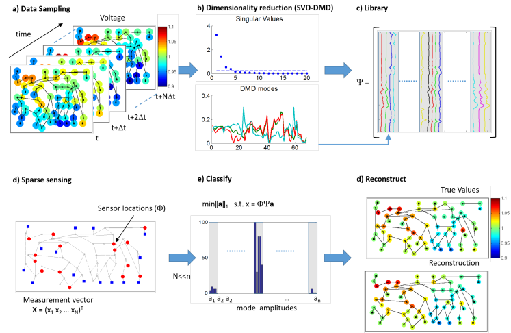
\par Figure~{}\ref{fig1} shows how the dimensionality reduction framework is combined with the compressive
sensing architecture. Specifically, simulations of the the IEEE 16-machine 68-bus Test System are used to
construct low-rank embeddings of the spatio-temporal activity in the Northeast United States. Dominant DMD modes
in various dynamic regimes are collected into a library of subspace embeddings via the matrix ${\bf\Psi}$. Since
a given dynamic regime only requires a sparse number of modes from ${\bf\Psi}$, compressive sensing can
be used to select the correct library elements for reconstruction and future state prediction. Thus the dimensionality
reduction and sparse sampling partner naturally for characterizing the power grid dynamics.
\par\par\par\@@numbered@section{section}{toc}{Power Systems Model}
\par\begin{table}\begin{tabular}[]{ccc}Area&Bus number&Total buses\\
\hline\cr 1&1-33, 113, 114, 115, 117&$m_{1}=37$\\
2&34-76, 116, 118&$m_{2}=45$\\
3&77-112&$m_{3}=36$\\
\hline\cr&&Total: $m_{T}=118$\end{tabular}
\@@toccaption{{\lx@tag[ ]{{1}}{Areas for the IEEE 118 Bus System}}}\@@caption{{\lx@tag[: ]{{Table 1}}{Areas for the IEEE 118 Bus System}}}\end{table}
\par To demonstrate the application of the proposed methodology on complex dynamical systems, we study the voltage profile of an IEEE test system model of a power system under disturbances. The IEEE test system is comprised of a 68-Bus, 16-machine, 5-Area System widely know in the power system literature. The IEEE 16-machine, 68-Bus test system is a reduced order equivalent of the interconnected New England test system (NETS) and New York power system (NYPS), with five geographical regions out of which NETS and NYPS are represented by a group of generators. The power imported from each of the three other neighboring areas (Quebec, Ontario and PJM) are approximated by equivalent generator models as shown in Figure 2. The NETS is represented by nine generators G1 to G9 and comprises the power system of the states of Maine, New Hampshire, Vermont, Massachuset, Connecticut and Rhode Island. The NYPS corresponds to power system of New York State and it is modeled by four generators G10 to G13. Generators G14 to G16 corresponds to the I-Quebec, II- Ontario and III-PJM regions.
\par\par\begin{figure}[t]
\includegraphics[width=238.49231pt]{Fig_3.pdf}
\@@toccaption{{\lx@tag[ ]{{3}}{Voltage profile of 68 buses at different regimes. After t=1 s there is a stable state, from t = 1 to t=1.01 the fault is applied (drop of voltage), and after t=1.01 the fault is cleared and the transient measurement is presented. }}}\@@caption{{\lx@tag[: ]{{Figure 3}}{Voltage profile of 68 buses at different regimes. After t=1 s there is a stable state, from t = 1 to t=1.01 the fault is applied (drop of voltage), and after t=1.01 the fault is cleared and the transient measurement is presented. }}}\vspace{-.15in}
\end{figure}
\par\begin{figure*}[t]
\includegraphics[width=368.57964pt]{fig_4.pdf}
\@@toccaption{{\lx@tag[ ]{{4}}{DMD modes representation of Regime 5 with threshold of 80\% of energy. The Mode 1 represents an exponential component with low damping, and higher values in buses close to the fault. Modes 2 and 3 represents an oscillatory mode with ? = 0.224 Hz and =-0.127.}}}\@@caption{{\lx@tag[: ]{{Figure 4}}{DMD modes representation of Regime 5 with threshold of 80\% of energy. The Mode 1 represents an exponential component with low damping, and higher values in buses close to the fault. Modes 2 and 3 represents an oscillatory mode with ? = 0.224 Hz and =-0.127.}}}
\end{figure*}
\par The bus data, line data, and detailed generator data of IEEE 16-machine 68-Bus test system are given in Ref.~{}\cite[cite]{\@@bibref{Authors Phrase1YearPhrase2}{rogers2012power}{\@@citephrase{(}}{\@@citephrase{)}}}. The test system is modeled using a subtransient reactance model for all generators and an IEEE type-II AVR for G1 to G8, meanwhile G9 is equipped with IEEE type-III AVR.
This system is chosen because it is a well-known and is a classic power system used for load flow analysis, small-signal stability analysis and non-linear simulation of the system. In our case, we use this model for non-linear simulations generated via software of power system transient analysis. The non-linear simulations are computed from the solution of the Differential-Algebraic Equations (DAE) used to represent the system. Here we are interested in the analysis of power system behavior under one of the most severe disturbance, a three-phase fault close to the bus-generator.
\par\par In order to test the performance of the proposed methodology, 16 disturbances were simulated in the closest bus to the generator, producing 16 distinct regimes. The disturbances, a three-phase fault at a respective bus, were introduced after one second of steady state operation and cleared after 0.1 seconds. Since the phenomenon of interest after the disruption are low frequency oscillations between 0.1 to 2 Hz, a time interval of 6 seconds is used to analyze the behavior of the system after fault clearance. The 6 second time window is sufficiently long so that at least a half cycle of the slowest oscillation can be captured. Typical voltage profiles of 68 buses for most representative regimes are shown in Fig. 3.
The voltage of 68 buses were sample at a rate of 100 Hz by every regime. We then consider the possibility of using only 10, 15, 20 and 30 buses for the identification, classification and reconstruction of the dynamic regime. Sensor placement algorithms are described in the next section.
\par\par\begin{figure*}[t]
\includegraphics[width=368.57964pt]{Fig_5.pdf}
\@@toccaption{{\lx@tag[ ]{{5}}{POD modes representation of Regime 5 with threshold of 80\% of energy. The Modes 1, 2 and 3 represents irregular oscillatory components whithin higher values in buses close to the fault.}}}\@@caption{{\lx@tag[: ]{{Figure 5}}{POD modes representation of Regime 5 with threshold of 80\% of energy. The Modes 1, 2 and 3 represents irregular oscillatory components whithin higher values in buses close to the fault.}}}
\end{figure*}
\par\par\begin{figure}[t]
\includegraphics[width=195.12767pt]{fig_6.pdf}
\@@toccaption{{\lx@tag[ ]{{6}}{Graph of sparse sensor placement on IEEE 16-machine 68-bus test system at different thresholds of energy (80\%, 90\%, 95\% and 99\%) for 10 and 20 sensors. The blue square represents the generators location. The red dots indicate the common sensor between thersholds energy and color circles shows independent sensors at every threshold}}}\@@caption{{\lx@tag[: ]{{Figure 6}}{Graph of sparse sensor placement on IEEE 16-machine 68-bus test system at different thresholds of energy (80\%, 90\%, 95\% and 99\%) for 10 and 20 sensors. The blue square represents the generators location. The red dots indicate the common sensor between thersholds energy and color circles shows independent sensors at every threshold}}}\vspace{-.15in}
\end{figure}
\par\par\begin{figure}[t]
\includegraphics[width=195.12767pt]{fig_7.pdf}
\@@toccaption{{\lx@tag[ ]{{7}}{Accuracy of sensor placement for the library at 80\% of energy at different time intervals and number of sensors considering a) Euclidean norm and b) Random sensor placement. There are considered a window of t=[0.1, 0.2, 0.4, 0.8, 1.4, 2.0, 3.0, 4.0] s. A 100 trials of random sensor placement are considered and the results are presented by boxplot in b) RND.}}}\@@caption{{\lx@tag[: ]{{Figure 7}}{Accuracy of sensor placement for the library at 80\% of energy at different time intervals and number of sensors considering a) Euclidean norm and b) Random sensor placement. There are considered a window of t=[0.1, 0.2, 0.4, 0.8, 1.4, 2.0, 3.0, 4.0] s. A 100 trials of random sensor placement are considered and the results are presented by boxplot in b) RND.}}}\vspace{-.15in}
\end{figure}
\par\begin{figure}[t]
\includegraphics[width=195.12767pt]{fig_8.pdf}
\@@toccaption{{\lx@tag[ ]{{8}}{Accuracy of sensor placement for the library at 99\% of energy at different time intervals and number of sensors considering a) Euclidean norm and b) Random sensor placement. There are considered a window of t=[0.1, 0.2, 0.4, 0.8, 1.4, 2.0, 3.0, 4.0] s. A 100 trials of random sensor placement are considered and the results are presented by boxplot in b) RND}}}\@@caption{{\lx@tag[: ]{{Figure 8}}{Accuracy of sensor placement for the library at 99\% of energy at different time intervals and number of sensors considering a) Euclidean norm and b) Random sensor placement. There are considered a window of t=[0.1, 0.2, 0.4, 0.8, 1.4, 2.0, 3.0, 4.0] s. A 100 trials of random sensor placement are considered and the results are presented by boxplot in b) RND}}}\vspace{-.15in}
\end{figure}
\par\par\par\begin{figure}[b]
\includegraphics[width=216.81pt]{fig_9.pdf}
\@@toccaption{{\lx@tag[ ]{{9}}{Voltage profile reconstruction of Regime 4 at t=1.54 s using 15 sensors and library of 80\% of energy. The upper image shows a graph of IEEE test system with voltage profiles values represented though circle?s diameter and colorbar.The middle images represents voltage profiles values as a colored bars for true values and reconstruction values. Finally the lower figure shows the difference between true values and reconstruction values.}}}\@@caption{{\lx@tag[: ]{{Figure 9}}{Voltage profile reconstruction of Regime 4 at t=1.54 s using 15 sensors and library of 80\% of energy. The upper image shows a graph of IEEE test system with voltage profiles values represented though circle?s diameter and colorbar.The middle images represents voltage profiles values as a colored bars for true values and reconstruction values. Finally the lower figure shows the difference between true values and reconstruction values.}}}\vspace{-.15in}
\end{figure}
\par\begin{figure}[t]
\includegraphics[width=216.81pt]{fig_10.pdf}
\@@toccaption{{\lx@tag[ ]{{10}}{Relative error for full voltage profile recontruction of all regimes at t=1.54 s using 15 and 20 sensors and library of 80\% of energy.}}}\@@caption{{\lx@tag[: ]{{Figure 10}}{Relative error for full voltage profile recontruction of all regimes at t=1.54 s using 15 and 20 sensors and library of 80\% of energy.}}}\vspace{-.15in}
\end{figure}
\par\par\par\@@numbered@section{section}{toc}{Power Systems Networks Dynamics}
\par The power system network dynamics are evaluated in two stages. During the first stage, a library of the dominant DMD modes all are extracted in order to determine a sensor placement. In the sparse measurement stage, the limited measurements are used to analyze, identify, classify and reconstruct the full voltages profiles of the power system.
\par\par\@@numbered@section{subsection}{toc}{Library Learning}
\par The 68-voltage measurements of every regime are analyzed by the DMD method to get a low dimensional representation of the data. DMD is used to construct a library of dominant DMD modes, which are the library elements that encode the low-rank dynamics of the power system for a specific regime or fault location.
\par\begin{table*}\begin{tabular}[]{c|rrrrrrrrrrrrrrrr|c}\hfil\lx@intercol\vrule\lx@intercol\hfil\lx@intercol&&&&&&{\bf DMD Regimes}&&&&&&&&&\lx@intercol\vrule\lx@intercol\hfil\lx@intercol&&\\[7.22743pt]
\hline\cr Threshold\hfil\lx@intercol\vrule\lx@intercol\hfil\lx@intercol&1&2&3&4&\color[rgb]{1,0,0} 5\color[rgb]{0,0,0}&6&7&8&9&10&11&12&13&14&15\lx@intercol\vrule\lx@intercol\hfil\lx@intercol&16&Library\\
\hfil\lx@intercol\vrule\lx@intercol\hfil\lx@intercol&&&&&&&&&&&&&&&\lx@intercol\vrule\lx@intercol\hfil\lx@intercol&&elements\\
\hline\cr 80\%\hfil\lx@intercol\vrule\lx@intercol\hfil\lx@intercol&2&3&2&2&\color[rgb]{1,0,0} 3\color[rgb]{0,0,0}&3&2&3&2&4&2&2&4&2&2\lx@intercol\vrule\lx@intercol\hfil\lx@intercol&2&40\\
90\%\hfil\lx@intercol\vrule\lx@intercol\hfil\lx@intercol&4&4&4&3&\color[rgb]{1,0,0} 4\color[rgb]{0,0,0}&4&3&5&3&6&4&4&5&3&3\lx@intercol\vrule\lx@intercol\hfil\lx@intercol&3&62\\
99\%\hfil\lx@intercol\vrule\lx@intercol\hfil\lx@intercol&10&11&11&8&\color[rgb]{1,0,0} 9\color[rgb]{0,0,0}&11&10&11&8&12&10&11&11&8&6\lx@intercol\vrule\lx@intercol\hfil\lx@intercol&8&155\end{tabular}{} {\rm(11)}\cr{\penalty 100\vskip 3.0pt\vskip 21.68121pt}
\begin{tabular}[]{c|rrrrrrrrrrrrrrrr|c}\hfil\lx@intercol\vrule\lx@intercol\hfil\lx@intercol&&&&&&{\bf POD Regimes}&&&&&&&&&\lx@intercol\vrule\lx@intercol\hfil\lx@intercol&&\\[7.22743pt]
\hline\cr Threshold\hfil\lx@intercol\vrule\lx@intercol\hfil\lx@intercol&1&2&3&4&\color[rgb]{1,0,0} 5\color[rgb]{0,0,0}&6&7&8&9&10&11&12&13&14&15\lx@intercol\vrule\lx@intercol\hfil\lx@intercol&16&Library\\
\hfil\lx@intercol\vrule\lx@intercol\hfil\lx@intercol&&&&&&&&&&&&&&&\lx@intercol\vrule\lx@intercol\hfil\lx@intercol&&elements\\
\hline\cr 80\%\hfil\lx@intercol\vrule\lx@intercol\hfil\lx@intercol&2&3&2&2&\color[rgb]{1,0,0} 3\color[rgb]{0,0,0}&3&2&3&2&4&2&2&4&2&2\lx@intercol\vrule\lx@intercol\hfil\lx@intercol&2&40\\
90\%\hfil\lx@intercol\vrule\lx@intercol\hfil\lx@intercol&4&4&4&3&\color[rgb]{1,0,0} 4\color[rgb]{0,0,0}&4&3&5&3&6&4&4&5&3&3\lx@intercol\vrule\lx@intercol\hfil\lx@intercol&3&62\\
99\%\hfil\lx@intercol\vrule\lx@intercol\hfil\lx@intercol&10&11&11&8&\color[rgb]{1,0,0} 9\color[rgb]{0,0,0}&11&10&11&8&12&10&11&11&8&6\lx@intercol\vrule\lx@intercol\hfil\lx@intercol&8&155\end{tabular}
\@@toccaption{{\lx@tag[ ]{{2}}{Number of modes for every regime using DMD method and POD method for a threshold 80\%, 90\% and 99\% of energy.}}}\@@caption{{\lx@tag[: ]{{Table 2}}{Number of modes for every regime using DMD method and POD method for a threshold 80\%, 90\% and 99\% of energy.}}}\end{table*}
\par The number of DMD modes choosen to be part of library are limited to those modes that captures a prescribed percentage of energy (or observed variance), based on singular values from the SVD computed during the DMD procedure. The full state voltage profiles are low-rank so that the dynamics of the power system can be represented by a sparse number of modes. These modes are called the dominant modes. Table 1 shows the number of DMD modes selected to represent every regime according to the energy threshold of 80\%, 90\% and 99\%. A comparison of the low dimensional representation between the DMD method and the POD modes is also presented in Table I.
Noticed that even when the number of modes for both methods are the same, their representation and meaning for the power network are different as it can be seen in Fig. 4 and Fig. 5.
\par\par\par\par\par\@@numbered@section{subsection}{toc}{Sparse Sensor Placement for Classification}
\par There are several ways to measure the importance of every sensor (or node) to the global behavior of the power system. A straightforward way is to measure the Euclidean norm between elements of library to rank every sensor. These projection onto the library elements give us an average of the importance of every sensor in the different regimes. The sensors can then be ordered from highest to lowest in the Euclidean norm, thus informing one of the number of sensors needed. The Fig. 6 shows a graph of sparse sensor placement on IEEE test system at different threshold of energy for the cases of 10 and 20 sensors.
\par\par Once the sparse sensor placement is defined, compressive sensing is used to identify, classify and reconstruct the full voltage profile of power system.
The identification and classification of every regime using a specific number of sensor are evaluating using the principles of compressive sensing outlined previously. The main assumption of compressed sensing in this context is that given measurement vector ${\bf y}={\bf\Phi\Psi a}$ is sparsely represented in ${\bf a}$. Thus the objective is to find a basis that represents our data ${\bf y}$ in a sparse manner based on $\min\|{\bf a}\|_{1}$ subject to ${\bf y=\Phi\Psi a}$. Once ${\bf a}$ is defined, the highest values of ${\bf a}$ corresponds to the element of the library associated with the selected regime.
The accuracy of proposed methodology in the identification and classification of regimes using a specific number of sensor is evaluated by averaging the identified regime of ${\bf y}$ every 5 samples until the number of samples corresponding to the window length i.e. for window length w = 0.1 s, there are 10 sample so the vector ${\bf a}$ is calculated twice. Then the average of all evaluations of a for every regime for every window length represents the accuracy of the proposed method. The results of these evaluations are shown in Fig. 7 and Fig. 8 when truncating the DMD library modes at 80\% and 99\% variance respectively.
\par In general, better accuracy is achieved for the sparse sensor placement algorithm using the Euclidean norm versus random sensor placement. Also when the sampling window length of $t$ reaches 0.8 and 1.4 seconds, the accuracy is effectively maximized. Thus, increasing the length of the sampling window does not improve performance. When 15 and 20 sensors are used, the accuracy achieves values of 70 to 90\% for both libraries.
In agreement with the previous analysis, a sparse sensor placement using 15 and 20 sensors and with a sampling window length of 1.4 seconds and library constructed with 80\% variance, reconstruction of full state is achieved. This selection implies a 77 and 88\% accuracy for the case of 15 and 20 sensors respectively.
\par\par\@@numbered@section{subsection}{toc}{Full State Reconstrution}
\par The full voltage profile reconstruction can be easily achieved once the classification task is accomplished. The procedure consists in projecting the data measurements onto the identified dominant modes of the library for the given regime found from classification.
The full sate reconstruction is considered using a window length of 1.4 seconds for the identification of the regime and 15 and 20 sparse sensors placed using the library with 80\% energy variance threshold. An example of the full voltage profile reconstruction is shown in Fig. 9. This reconstruction corresponds to the worst case of all regimes and the values of the difference between the true values and reconstruction values are located in the buses close to the fault. Even when this values exist, they are meaningless.
\par The relative error of full voltage profile reconstruction of all regimes at a specific snapshot using 15 and 20 sensors and library of 80\% variance is displayed in Fig. 10. Noticed that higher values of relative error for 15 sensors belongs to R4, R8, R14 and R16, which suggests that four modes could not easily be correctly identified. However, the values of relative error for most of buses of these regimes remain at low levels. These results are improved when we use 20 sensors instead of 15 sensors. In this case, there are only two regimes with errors, R14 an R16. This results shown in Fig. 10 agrees with the accuracy results of Fig. 7.
\par\par\@@numbered@section{section}{toc}{Conclusions}
\par This paper proposes a data-driven framework for the analysis and visualization of power system disturbances. The approach is based on a semi-distributed algorithm that allows the computation of energy-based metrics from extracted consensus components. Specifically, we have further developed the DMD algorithm for characterizing the dynamics of disturbances in power grid networks and monitoring wide-area power grid networks from sparse measurement data.
Our proposed data-driven strategy, which is based on energy metrics, can be used for the analysis of major disturbances in the network. The approach is tested and validated using time domain simulations in the IEEE 118 bus system under various disturbance scenarios and under different sparse observations of the system. In addition to state reconstruction, the minimal number of sensors required for monitoring disturbances can be evaluated. Visualization techniques are developed in order to aid in the analysis and characterization of the system after disturbance.
\par With the emergence of advanced wide-area monitoring of power grid systems, it is important to develop data-driven methods that can continuously assess the power system health and performance. Central to such monitoring schemes are intelligent sensing methods, signal processing and communication technologies to make optimal use of measured wide-area data. We propose a new methodology for converting sparse, real-time measurements of a power grid into useful information that can be used to reconstruct the entire state space and produce short-time forecasts. The utility of such algorithms are central to timely detection and display of adverse conditions in the power grid. We have shown that the recently developed {\em dynamic mode decomposition} (DMD) is a promising data-driven method that allows for full state-space reconstruction and forecasting with limited measurements of the power grid system, thus enabling real-time monitoring capabilities.
\par\par\@@unnumbered@section{section}{}{Acknowledgements}
JJR acknowledges support from National Council for Science and Technology of Mexico (CONACyT) under the grant No. 290733 and Cinvestav IPN. JNK acknowledges support from the U.S. Air Force Office of Scientific Research (FA9550-19-1-0011).
\par\par\par\par
\footnotesize{
\thebibliography
\@@lbibitem{messina2015wide}\NAT@@wrout{1}{2015}{Messina and Messina}{}{Messina and Messina [2015]}{messina2015wide}\lx@bibnewblock
A.~{}R. Messina and
A.~{}R. Messina,
\emph{Wide-area monitoring of interconnected power systems}
(The Institution of Engineering and Technology,
2015).
\par\@@lbibitem{kezunovic2013role}\NAT@@wrout{2}{2013}{Kezunovic et~{}al.}{Kezunovic, Xie,
and Grijalva}{Kezunovic et~{}al. [2013]}{kezunovic2013role}\lx@bibnewblock
M.~{}Kezunovic,
L.~{}Xie, and
S.~{}Grijalva, in
\emph{Bulk Power System Dynamics and Control-IX
Optimization, Security and Control of the Emerging Power Grid (IREP), 2013
IREP Symposium} (IEEE, 2013), pp.
1--9.
\par\@@lbibitem{barocio2013detection}\NAT@@wrout{3}{2013}{Barocio et~{}al.}{Barocio, Pal,
Fabozzi, and Thornhill}{Barocio et~{}al. [2013]}{barocio2013detection}\lx@bibnewblock
E.~{}Barocio,
B.~{}C. Pal,
D.~{}Fabozzi, and
N.~{}F. Thornhill, in
\emph{Bulk Power System Dynamics and Control-IX
Optimization, Security and Control of the Emerging Power Grid (IREP), 2013
IREP Symposium} (IEEE, 2013), pp.
1--10.
\par\@@lbibitem{susuki2009global}\NAT@@wrout{4}{2009}{Susuki et~{}al.}{Susuki, Mezic, and
Hikihara}{Susuki et~{}al. [2009]}{susuki2009global}\lx@bibnewblock
Y.~{}Susuki,
I.~{}Mezic, and
T.~{}Hikihara, in
\emph{2009 American Control Conference}
(IEEE, 2009), pp.
3446--3451.
\par\@@lbibitem{susuki2011coherent}\NAT@@wrout{5}{2011}{Susuki et~{}al.}{Susuki, Mezi{\'{c}},
and Hikihara}{Susuki et~{}al. [2011]}{susuki2011coherent}\lx@bibnewblock
Y.~{}Susuki,
I.~{}Mezi{\'{c}},
and T.~{}Hikihara,
Journal of nonlinear science
{21}, 403 (2011).
\par\@@lbibitem{susuki2011nonlinear}\NAT@@wrout{6}{2011}{Susuki and Mezic}{}{Susuki and Mezic [2011]}{susuki2011nonlinear}\lx@bibnewblock
Y.~{}Susuki and
I.~{}Mezic,
IEEE Transactions on Power Systems
{26}, 1894 (2011).
\par\@@lbibitem{susuki2012nonlinear}\NAT@@wrout{7}{2012}{Susuki and Mezic}{}{Susuki and Mezic [2012]}{susuki2012nonlinear}\lx@bibnewblock
Y.~{}Susuki and
I.~{}Mezic,
IEEE Transactions on Power Systems
{27}, 1182 (2012).
\par\@@lbibitem{susuki2014nonlinear}\NAT@@wrout{8}{2014}{Susuki and Mezi{\'{c}}}{}{Susuki and Mezi{\'{c}} [2014]}{susuki2014nonlinear}\lx@bibnewblock
Y.~{}Susuki and
I.~{}Mezi{\'{c}},
IEEE Transactions on Power Systems
{29}, 899 (2014).
\par\@@lbibitem{li2010online}\NAT@@wrout{9}{2010}{Li et~{}al.}{Li, Tang, Ma, and
Liu}{Li et~{}al. [2010]}{li2010online}\lx@bibnewblock
W.~{}Li,
J.~{}Tang,
J.~{}Ma, and
Y.~{}Liu, IEEE
Transactions on Smart Grid {1},
253 (2010).
\par\@@lbibitem{mei2008clustering}\NAT@@wrout{10}{2008}{Mei et~{}al.}{Mei, Rovnyak, and
Ong}{Mei et~{}al. [2008]}{mei2008clustering}\lx@bibnewblock
K.~{}Mei,
S.~{}M. Rovnyak,
and C.-M. Ong,
IEEE Transactions on Power Systems
{23}, 673 (2008).
\par\@@lbibitem{bhui2016application}\NAT@@wrout{11}{2016}{Bhui and Senroy}{}{Bhui and Senroy [2016]}{bhui2016application}\lx@bibnewblock
P.~{}Bhui and
N.~{}Senroy,
IEEE Transactions on Power Systems
{31}, 581 (2016).
\par\@@lbibitem{shahraeini2011comparison}\NAT@@wrout{12}{2011}{Shahraeini et~{}al.}{Shahraeini,
Javidi, and Ghazizadeh}{Shahraeini et~{}al. [2011]}{shahraeini2011comparison}\lx@bibnewblock
M.~{}Shahraeini,
M.~{}H. Javidi,
and M.~{}S.
Ghazizadeh, IEEE Transactions on Smart Grid
{2}, 206 (2011).
\par\@@lbibitem{wang2015decentralized}\NAT@@wrout{13}{2015}{Wang et~{}al.}{Wang, Yemula, and
Bose}{Wang et~{}al. [2015]}{wang2015decentralized}\lx@bibnewblock
Y.~{}Wang,
P.~{}Yemula, and
A.~{}Bose,
IEEE Transactions on Smart Grid
{6}, 885 (2015).
\par\@@lbibitem{ning2013oscillation}\NAT@@wrout{14}{2013}{Ning et~{}al.}{Ning, Pan, and
Venkatasubramanian}{Ning et~{}al. [2013]}{ning2013oscillation}\lx@bibnewblock
J.~{}Ning,
X.~{}Pan, and
V.~{}Venkatasubramanian,
IEEE Transactions on Power Systems
{28}, 1960 (2013).
\par\@@lbibitem{khalid2015improved}\NAT@@wrout{15}{2015}{Khalid and Peng}{}{Khalid and Peng [2015]}{khalid2015improved}\lx@bibnewblock
H.~{}M. Khalid and
J.~{}C.-H. Peng,
IEEE Transactions on Power Systems
{30}, 680 (2015).
\par\@@lbibitem{nabavi2015distributed}\NAT@@wrout{16}{2015}{Nabavi et~{}al.}{Nabavi, Zhang, and
Chakrabortty}{Nabavi et~{}al. [2015]}{nabavi2015distributed}\lx@bibnewblock
S.~{}Nabavi,
J.~{}Zhang, and
A.~{}Chakrabortty,
IEEE Transactions on Smart Grid
{6}, 2529 (2015).
\par\@@lbibitem{eriksson2011wide}\NAT@@wrout{17}{2011}{Eriksson and Soder}{}{Eriksson and Soder [2011]}{eriksson2011wide}\lx@bibnewblock
R.~{}Eriksson and
L.~{}Soder,
IEEE Transactions on Power Delivery
{26}, 988 (2011).
\par\@@lbibitem{liu2015armax}\NAT@@wrout{18}{2015}{Liu et~{}al.}{Liu, Zhu, Pan, Bai, Liu,
Liu, Patel, Farantatos, and Bhatt}{Liu et~{}al. [2015]}{liu2015armax}\lx@bibnewblock
H.~{}Liu,
L.~{}Zhu,
Z.~{}Pan,
F.~{}Bai,
Y.~{}Liu,
Y.~{}Liu,
M.~{}Patel,
E.~{}Farantatos,
and N.~{}Bhatt
(2015).
\par\@@lbibitem{Pearson:1901}\NAT@@wrout{19}{1901}{Pearson}{}{Pearson [1901]}{Pearson:1901}\lx@bibnewblock
K.~{}Pearson,
Philosophical Magazine {2},
559 (1901).
\par\@@lbibitem{hotellingJEdPsy33_1}\NAT@@wrout{20}{1933{a}}{Hotelling}{}{Hotelling [1933{a}]}{hotellingJEdPsy33_1}\lx@bibnewblock
H.~{}Hotelling,
{24}, 417
(1933{a}), ISSN 0022-0663.
\par\@@lbibitem{hotellingJEdPsy33_2}\NAT@@wrout{21}{1933{b}}{Hotelling}{}{Hotelling [1933{b}]}{hotellingJEdPsy33_2}\lx@bibnewblock
H.~{}Hotelling,
{24}, 498
(1933{b}), ISSN 0022-0663.
\par\@@lbibitem{eof1}\NAT@@wrout{22}{1956}{Lorenz}{}{Lorenz [1956]}{eof1}\lx@bibnewblock
E.~{}N. Lorenz,
Technical report, Massachusetts Institute of Technology
{Dec.} (1956).
\par\@@lbibitem{Berkooz:1993}\NAT@@wrout{23}{1993}{Berkooz et~{}al.}{Berkooz, Holmes, and
Lumley}{Berkooz et~{}al. [1993]}{Berkooz:1993}\lx@bibnewblock
G.~{}Berkooz,
P.~{}Holmes, and
J.~{}L. Lumley,
Annual Review of Fluid Mechanics
{23}, 539 (1993).
\par\@@lbibitem{HLBR_turb}\NAT@@wrout{24}{2012}{Holmes et~{}al.}{Holmes, Lumley,
Berkooz, and Rowley}{Holmes et~{}al. [2012]}{HLBR_turb}\lx@bibnewblock
P.~{}J. Holmes,
J.~{}L. Lumley,
G.~{}Berkooz, and
C.~{}W. Rowley,
\emph{Turbulence, coherent structures, dynamical systems and
symmetry}, Cambridge Monographs in Mechanics (Cambridge
University Press, Cambridge, England,
2012), 2nd ed.
\par\@@lbibitem{manohar2017data}\NAT@@wrout{25}{2017}{Manohar et~{}al.}{Manohar, Brunton,
Kutz, and Brunton}{Manohar et~{}al. [2017]}{manohar2017data}\lx@bibnewblock
K.~{}Manohar,
B.~{}W. Brunton,
J.~{}N. Kutz, and
S.~{}L. Brunton,
arXiv preprint arXiv:1701.07569 (2017).
\par\@@lbibitem{sirovich1995}\NAT@@wrout{26}{1995}{Everson and Sirovich}{}{Everson and Sirovich [1995]}{sirovich1995}\lx@bibnewblock
R.~{}Everson and
L.~{}Sirovich,
J. Opt. Soc. Am. A {12},
1657 (1995).
\par\@@lbibitem{willcox2005}\NAT@@wrout{27}{2006}{Willcox}{}{Willcox [2006]}{willcox2005}\lx@bibnewblock
K.~{}Willcox,
Computers \& Fluids {35},
208 (2006).
\par\@@lbibitem{Yildirim:2009}\NAT@@wrout{28}{2009}{Yildirim et~{}al.}{Yildirim,
Chryssostomidis, and Karniadakis}{Yildirim et~{}al. [2009]}{Yildirim:2009}\lx@bibnewblock
B.~{}Yildirim,
C.~{}Chryssostomidis,
and G.~{}E.
Karniadakis, Ocean Modelling
{27}, 160 (2009).
\par\@@lbibitem{sorensen2010}\NAT@@wrout{29}{2010}{Chaturantabut and Sorensen}{}{Chaturantabut and Sorensen [2010]}{sorensen2010}\lx@bibnewblock
S.~{}Chaturantabut
and D.~{}C.
Sorensen, SIAM J. Sci. Comput.
{32}, 2737 (2010).
\par\@@lbibitem{sargsyan2015}\NAT@@wrout{30}{2015}{Sargsyan et~{}al.}{Sargsyan, Brunton,
and Kutz}{Sargsyan et~{}al. [2015]}{sargsyan2015}\lx@bibnewblock
S.~{}Sargsyan,
S.~{}L. Brunton,
and J.~{}N. Kutz,
Phys. Rev. E {92},
033304 (2015).
\par\@@lbibitem{Schmid2010jfm}\NAT@@wrout{31}{2010}{Schmid}{}{Schmid [2010]}{Schmid2010jfm}\lx@bibnewblock
P.~{}J. Schmid,
Journal of Fluid Mechanics {656},
5 (2010), ISSN 0022-1120.
\par\@@lbibitem{Brunton2015jcd}\NAT@@wrout{32}{2015}{Brunton et~{}al.}{Brunton, Proctor,
Tu, and Kutz}{Brunton et~{}al. [2015]}{Brunton2015jcd}\lx@bibnewblock
S.~{}L. Brunton,
J.~{}L. Proctor,
J.~{}H. Tu, and
J.~{}N. Kutz
(2015), to appear in the Journal of
Computational Dynamics. Available: arXiv:1312.5186.
\par\@@lbibitem{Tu:2014b}\NAT@@wrout{33}{2014{a}}{Tu et~{}al.}{Tu, Rowley,
Kutz, and Shang}{Tu et~{}al. [2014{a}]}{Tu:2014b}\lx@bibnewblock
J.~{}H. Tu,
C.~{}W. Rowley,
J.~{}N. Kutz, and
J.~{}K. Shang,
Experiments in Fluids {55},
1 (2014{a}).
\par\@@lbibitem{askham2018variable}\NAT@@wrout{34}{2018}{Askham and Kutz}{}{Askham and Kutz [2018]}{askham2018variable}\lx@bibnewblock
T.~{}Askham and
J.~{}N. Kutz,
SIAM Journal on Applied Dynamical Systems
{17}, 380 (2018).
\par\@@lbibitem{Tu2014jcd}\NAT@@wrout{35}{2014{b}}{Tu et~{}al.}{Tu, Rowley,
Luchtenburg, Brunton, and Kutz}{Tu et~{}al. [2014{b}]}{Tu2014jcd}\lx@bibnewblock
J.~{}H. Tu,
C.~{}W. Rowley,
D.~{}M. Luchtenburg,
S.~{}L. Brunton,
and J.~{}N. Kutz,
Journal of Computational Dynamics
{1}, 391
(2014{b}).
\par\@@lbibitem{mezic2013analysis}\NAT@@wrout{36}{2013}{Mezic}{}{Mezic [2013]}{mezic2013analysis}\lx@bibnewblock
I.~{}Mezic,
Annual Review of Fluid Mechanics
{45}, 357 (2013).
\par\@@lbibitem{DMDbook}\NAT@@wrout{37}{2016}{Kutz et~{}al.}{Kutz, Brunton, Brunton,
and Proctor}{Kutz et~{}al. [2016]}{DMDbook}\lx@bibnewblock
J.~{}N. Kutz,
S.~{}L. Brunton,
B.~{}W. Brunton,
and J.~{}L.
Proctor, \emph{Dynamic mode decomposition:
Data-driven modeling of complex systems} (2016).
\par\@@lbibitem{bright2013}\NAT@@wrout{38}{2013}{Bright et~{}al.}{Bright, Lin, and
Kutz}{Bright et~{}al. [2013]}{bright2013}\lx@bibnewblock
I.~{}Bright,
G.~{}Lin, and
J.~{}N. Kutz,
Phys. Fluids {25},
127102 (2013).
\par\@@lbibitem{Brunton2014siads}\NAT@@wrout{39}{2014}{Brunton et~{}al.}{Brunton, Tu, Bright,
and Kutz}{Brunton et~{}al. [2014]}{Brunton2014siads}\lx@bibnewblock
S.~{}L. Brunton,
J.~{}H. Tu,
I.~{}Bright, and
J.~{}N. Kutz,
SIAM Journal on Applied Dynamical Systems
{13}, 1716 (2014).
\par\@@lbibitem{Proctor2014epj}\NAT@@wrout{40}{2014}{Proctor et~{}al.}{Proctor, Brunton,
Brunton, and Kutz}{Proctor et~{}al. [2014]}{Proctor2014epj}\lx@bibnewblock
J.~{}L. Proctor,
S.~{}L. Brunton,
B.~{}W. Brunton,
and J.~{}N. Kutz,
The European Physical Journal Special Topics
{223}, 2665 (2014).
\par\@@lbibitem{kramer}\NAT@@wrout{41}{2015}{Kramer et~{}al.}{Kramer, Grover,
Boufounos, Benosman, and Nabi}{Kramer et~{}al. [2015]}{kramer}\lx@bibnewblock
B.~{}Kramer,
P.~{}Grover,
P.~{}Boufounos,
M.~{}Benosman, and
S.~{}Nabi,
arXiv preprint arXiv:1510.02831 (2015).
\par\@@lbibitem{Candes:2006c}\NAT@@wrout{42}{59}{Cand\`{e}s et~{}al.}{Cand\`{e}s, Romberg,
and Tao}{Cand\`{e}s et~{}al. [59]}{Candes:2006c}\lx@bibnewblock
E.~{}J. Cand\`{e}s,
J.~{}Romberg, and
T.~{}Tao,
Communications in Pure and Applied Mathematics
{8} (59).
\par\@@lbibitem{Donoho:2006}\NAT@@wrout{43}{2006}{Donoho}{}{Donoho [2006]}{Donoho:2006}\lx@bibnewblock
D.~{}L. Donoho,
IEEE Transactions on Information Theory
{52}, 1289 (2006).
\par\@@lbibitem{tropp2007signal}\NAT@@wrout{44}{2007}{Tropp and Gilbert}{}{Tropp and Gilbert [2007]}{tropp2007signal}\lx@bibnewblock
J.~{}A. Tropp and
A.~{}C. Gilbert,
IEEE Transactions on information theory
{53}, 4655 (2007).
\par\@@lbibitem{Candes:2006}\NAT@@wrout{45}{2006}{Cand\`{e}s}{}{Cand\`{e}s [2006]}{Candes:2006}\lx@bibnewblock
E.~{}J. Cand\`{e}s,
Proceedings of the International Congress of Mathematics
(2006).
\par\@@lbibitem{Candes:2006a}\NAT@@wrout{46}{2006}{Cand\`{e}s et~{}al.}{Cand\`{e}s, Romberg,
and Tao}{Cand\`{e}s et~{}al. [2006]}{Candes:2006a}\lx@bibnewblock
E.~{}J. Cand\`{e}s,
J.~{}Romberg, and
T.~{}Tao, IEEE
Transactions on Information Theory {52},
489 (2006).
\par\@@lbibitem{Baraniuk:2007}\NAT@@wrout{47}{2007}{Baraniuk}{}{Baraniuk [2007]}{Baraniuk:2007}\lx@bibnewblock
R.~{}G. Baraniuk,
IEEE Signal Processing Magazine
{24}, 118 (2007).
\par\@@lbibitem{Candes:2006b}\NAT@@wrout{48}{2006}{Cand\`{e}s and Tao}{}{Cand\`{e}s and Tao [2006]}{Candes:2006b}\lx@bibnewblock
E.~{}J. Cand\`{e}s and
T.~{}Tao, IEEE
Transactions on Information Theory {52},
5406 (2006).
\par\@@lbibitem{rogers2012power}\NAT@@wrout{49}{2012}{Rogers}{}{Rogers [2012]}{rogers2012power}\lx@bibnewblock
G.~{}Rogers,
\emph{Power system oscillations}
(Springer Science \& Business Media,
2012).
\par\endthebibliography
}
\par\@add@PDF@RDFa@triples\par\end{document}}}}}}}}}}}}}