The runaway greenhouse radius inflation effect

Planets similar to Earth – but slightly more irradiated – are expected to enter into a runaway greenhouse state, where all surface water rapidly evaporates, forming an optically thick H₂O-dominated atmosphere. For Earth, this extreme climate transition is thought to occur for a $\sim$ 6$\%$ increase only of the solar luminosity, though the exact limit at which the transition would occur is still a highly debated topic. In general, the runaway greenhouse is believed to be a fundamental process in the evolution of Earth-size, temperate planets. Using 1-D radiative-convective climate calculations accounting for thick, hot water vapour-dominated atmospheres, we evaluate the transit atmospheric thickness of a post-runaway greenhouse atmosphere, and find that it could possibly reach over a thousand kilometers (i.e., a few tens of $\%$ of Earth radius). This abrupt radius inflation – resulting from the runaway-greenhouse-induced transition – could be detected statistically by ongoing and upcoming space missions such as TESS, CHEOPS and PLATO (combined with precise radial velocity mass measurements with ground-based spectrographs such as ESPRESSO, CARMENES or SPIRou), or even in particular cases in multiplanetary systems such as TRAPPIST-1 (when masses and radii will be known with good enough precision). This result provides the community with an observational test of (1) the concept of runaway greenhouse, that defines the inner edge of the traditional Habitable Zone, and the exact limit of the runaway greenhouse transition. In particular, this could provide an empirical measurement of the irradiation at which Earth analogs transition from a temperate to a runaway greenhouse climate state. This astronomical measurement would make it possible to statistically estimate how close Earth is from the runaway greenhouse. (2) the presence (and statistical abundance) of water in temperate, Earth-size exoplanets.

1 Introduction

Planets similar to Earth – but slightly more irradiated – are expected to experience a runaway greenhouse transition, a state in which a net positive feedback between surface temperature, evaporation, and atmospheric opacity causes a runaway warming (Ingersoll, 1969; Goldblatt & Watson, 2012). This runaway greenhouse positive feedback ceases only when oceans have completely boiled away, forming an optically thick H₂O-dominated atmosphere. Venus may have experienced a runaway greenhouse in the past (Rasool & de Bergh, 1970; Kasting et al., 1984), and we expect that Earth will in around 600 million years as solar luminosity increases by $\sim$ 6$\%$ compared to its present-day value (Gough, 1981). However, the exact limit at which this extreme, rapid climate transition from a temperate climate (with most water condensed on the surface) to a post-runaway greenhouse climate (with all water in the atmosphere) would occur, and whether or not a CO₂ atmospheric level increase would affect that limit, is still a highly debated topic (Leconte et al., 2013; Goldblatt et al., 2013; Ramirez et al., 2014; Popp et al., 2016). This runaway greenhouse limit is traditionally used to define the inner edge of the Habitable Zone (Kasting et al., 1993; Kopparapu et al., 2013).

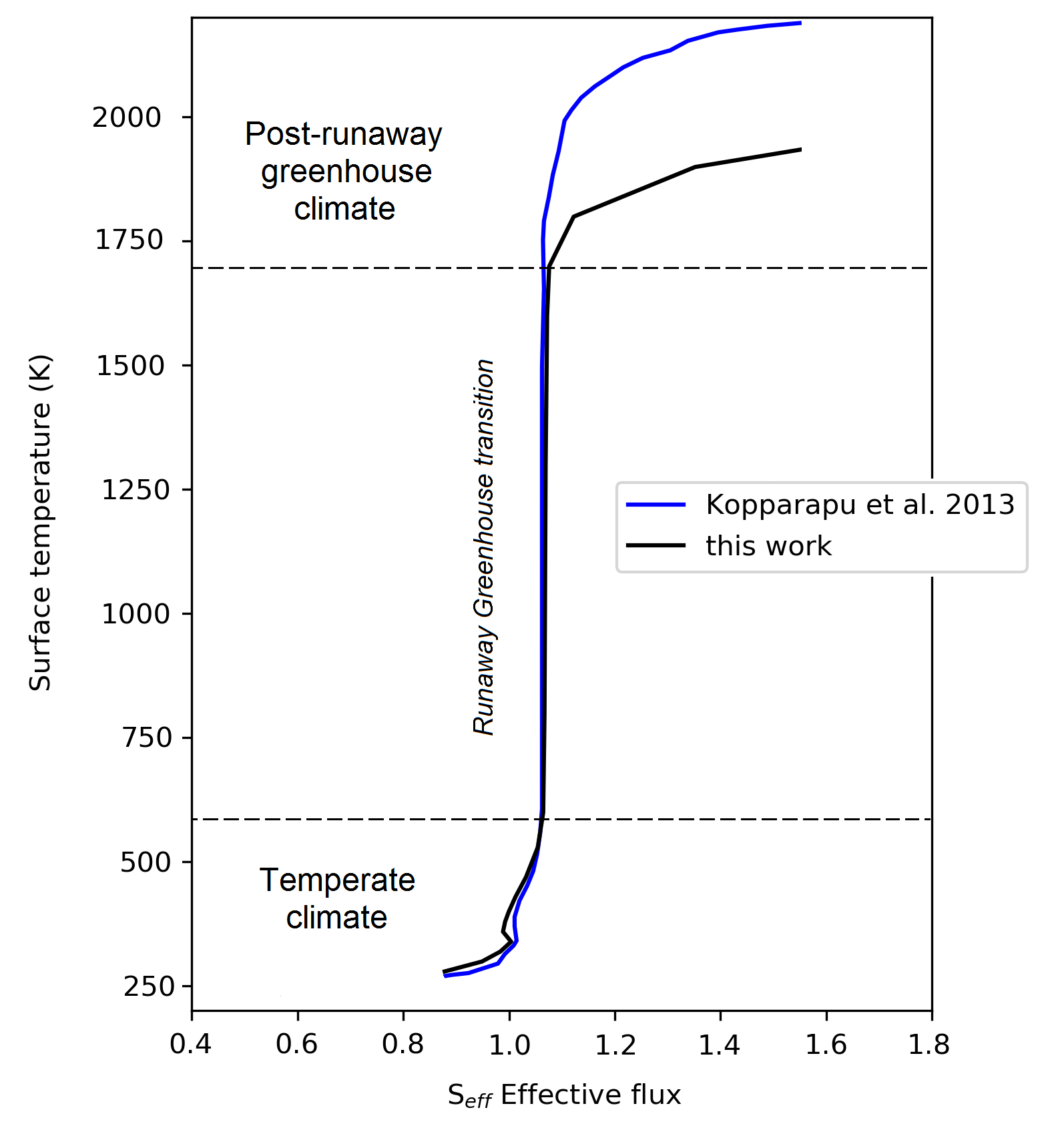
Figure 1: Surface temperature of the planet calculated as a function of the effective flux S${}_{\text{eff}}$, defined as the stellar flux received by the planet relative to present-day Earth solar flux. Here we compare the results of our climate calculations (black line) with those presented in the Figure 3c of Kopparapu et al. 2013 (blue line).

Here we take advantage of this runaway greenhouse process to propose a new, innovative observational test of the Habitable Zone concept, that could also be used to constrain the presence (and statistical abundance) of water in temperate, Earth-size exoplanets.

2 The runaway greenhouse radius inflation effect

Here we use a 1-D radiative-convective version of the LMD Generic model, that has already been used to simulate the runaway greenhouse process on Earth, Mars and exoplanets (Leconte et al., 2013; Turbet et al., 2019). Our 1D version of the LMD Generic inverse model is a single-column inverse radiative-convective climate model following the same approach (inverse modeling) as in Kasting et al. (1984) and more recently as in Kopparapu et al. (2013). More details on the model can be found in Appendix A.

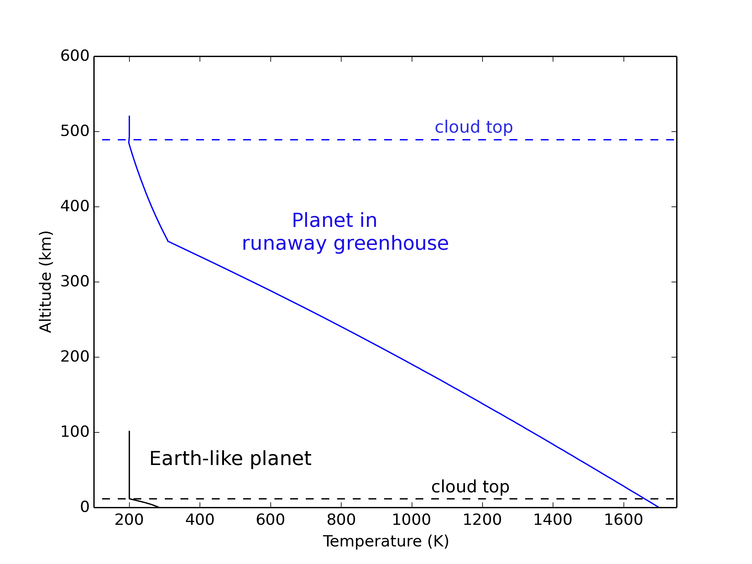
Figure 2: Thermal profiles of an Earth-like planet receiving the same insolation than present-day Earth (solid black curve) and receiving 6$\%$ more insolation than Earth (solid blue curve). In the latter case, the planet is in a post-runaway greenhouse climate state. The top of the cloud layer – estimated using the top of the moist convective layer – is indicated with dashed lines.

We use this model to simulate how the climate of an Earth-like planet – covered with a water reservoir equal to that of the Earth ocean water content – evolves as a function of stellar irradiation (Fig. 1), following the same methodology than used in Kasting et al. (1993) or more recently in Kopparapu et al. (2013). We recover the results of Kopparapu et al. (2013) that an Earth-like planet would experience a runaway greenhouse transition for an insolation equal to $\sim$ 1.06 times that of Earth. Moreover, we calculate that a planet experiencing the runaway greenhouse would start to equilibrate – in a post-runaway greenhouse climate state – for a surface temperature of $\sim$ 1700 K, i.e. only 100 K lower than reported in Kopparapu et al. (2013). This difference is likely due to the use of different H₂O- continuum databases, i.e. BPS (Paynter & Ramaswamy, 2011) versus MT$\_$CKD (Mlawer et al., 2012) here.

Fig. 2 shows the calculated thermal profiles for an Earth-like planet receiving an insolation equal to that of present-day Earth (black line; temperate climate state) and receiving an insolation equal to 1.07 times that of present-day Earth (blue line; post-runaway greenhouse climate state). Fig. 2 illustrates our main finding that as an Earth-like planet evolves from a temperate to a post-runaway greenhouse climate state, the apparent thickness of its atmosphere evolves from almost zero up to 500 km. Note that the same effect can qualitatively be observed in the Figure 1 of Goldblatt (2015), using a different 1-D numerical climate model. The apparent thickness of the planetary atmospheres is defined here as the top of the cloud layer (assumed to be optically thick), but we show in Section 3 that this result is nearly unchanged when a cloud-free atmosphere is assumed. The transition from a temperate to a post-runaway greenhouse climate would thus produce a $\sim$ 500 km radius increase. We call this phenomenon the runaway greenhouse radius inflation effect.

There are at least four distinct causes that cumulatively produce this radius inflation:

1. The total mass of the atmosphere increases by a factor of $\sim$ 270 (from 1 to $\sim$270 bars, i.e. the estimated surface pressure if the Earth ocean water content is entirely vaporized in the atmosphere).

2. The atmosphere becomes much hotter, which increases the atmospheric scale height H = $\frac{RT}{\mu g}$ (with $R$ the ideal gas constant, $T$ the temperature, $\mu$ the mean molecular mass and $g$ the gravity).

3. The atmosphere is now optically thick at much lower atmospheric pressure, because – for a given atmospheric pressure – the temperature is much higher, thus increasing the water vapour mixing ratio. This increases in turn (i) the water vapour absorption in the upper atmosphere and (ii) the altitude of the top of the cloud layer.

4. The mean molecular mass $\mu$ decreases (N₂ and O₂ are heavier than H₂O), which increases the atmospheric scale height.

While for Earth the net radius increase is about 500 km, we actually find that the radius increase significantly changes depending on the water content. This is explored in the next section.

3 Dependence on water content

The Earth near-surface and surface water reservoir is equal to 1.3$\times$10²¹ kg, or 2.7 km GEL (Global Equivalent Layer; i.e. the globally averaged depth of the layer that would result from putting all the water at the surface in a liquid phase), or 270 bars (Equivalent water vapour atmospheric pressure if the entire water reservoir is vaporized in the atmosphere), or 0.022$\%$ of the total Earth mass. But Earth-size planets can potentially have a very different water content than Earth (Raymond et al., 2004; Léger et al., 2004; Tian & Ida, 2015). Some planets may have started with a low water reservoir and may have lost most of it through atmospheric escape (e.g. during the runaway and post-runaway greenhouse phase, where water vapour is the dominant gas and is thus exposed to photodissociation and subsequent atmospheric escape). This is likely what happened to Venus (see the introduction section of Way et al. 2016 for a recent review). But some others may have started with a lot of water and retained most of it through their evolution.

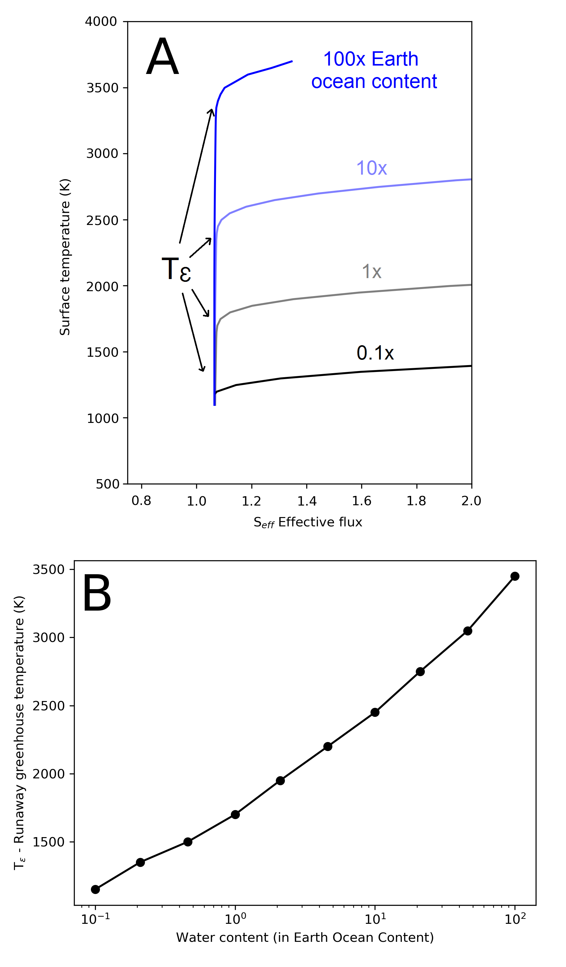
Figure 3: Top panel (A): Surface temperature of the planet calculated as a function of the effective flux S${}_{\text{eff}}$ (defined as the stellar flux received by the planet relative to present-day Earth solar flux), for 4 distinct total water contents (0.1, 1, 10 and 100 times the Earth ocean water content). Bottom panel (B): Runaway greenhouse temperature (T_ϵ) as a function of the total water content. Our best fit is obtained for T${}_{\epsilon}(Wc)$ = 80 $\Big{(}\log_{10}{Wc}\Big{)}^{2}$+700 $\Big{(}\log_{10}{Wc}\Big{)}$+1700, with $Wc$ the water content in Earth ocean water content units.

Using our 1D climate model (see Appendix A), we calculate thermal profiles of Earth-like planets in both temperate and post-runaway greenhouse climate states, and for a large range of water contents (from 0.1 to 100 times the Earth ocean water content), in order to study how water content changes the amplitude of the runaway greenhouse radius inflation effect. For this, we use the following procedure:

Step 1 -

For a wide range of total water content (from 0.1 to 100$\times$ that of the present-day Earth water ocean content) and a wide range of surface temperatures (from 200 to 4000 K), we construct the atmospheric thermal profile (temperature and water vapour mixing ratio) using the 1D LMD Generic model described in Appendix A.

Step 2 -

For each thermal profile, we perform the radiative transfer (see Appendix A) and compute the effective flux S${}_{\text{eff}}$, defined as the stellar flux (relative to the solar flux received by present-day Earth) necessary for each simulated planetary atmosphere to be in radiative equilibrium (see Appendix A). Note that we did not account for the radius inflation effect in these radiative transfer calculations for steam atmospheres, originating from the fact that the average radius for thermal emission can vary significantly from the average radius for absorption of solar radiation. However, Goldblatt (2015) showed that this effect should not affect more than 5$\%$ of the flux to which a planet undergoes the runaway greenhouse transition, for a planet the size and mass similar to the Earth.

Step 3 -

We calculate the threshold temperature T_ϵ (Marcq et al., 2017), defined here as the surface temperature at which the effective flux S${}_{\text{eff}}$ (i.e. the stellar flux received by the planet, relative to present-day Earth solar flux, needed for a planet to reach radiative equilibrium for a given surface temperature) changes from a constant runaway greenhouse regime to a post-runaway regime for which the effective flux S${}_{\text{eff}}$ starts to significantly increase with surface temperature (see Fig. 3A). T_ϵ is used here to define the surface temperature at which a planet that experienced a runaway greenhouse transition roughly starts to equilibrate.

Fig. 3B shows how the threshold temperature T_ϵ – defining the surface temperature of the post-runaway greenhouse atmosphere – varies as a function of water content. We find that the threshold temperature increases significantly with the water content, qualitatively recovering the results of Marcq et al. (2017) and Ikoma et al. (2018). The higher the water content, the more opaque the H₂O-rich lower atmosphere, the higher the surface temperature needs to be to radiate in the visible spectral domain (where H₂O is a weak absorber, but also a weak emitter), allowing the planet to radiatively equilibrate.

Step 4 -

We calculate the thermal and water vapour mixing ratio profiles of the post-runaway greenhouse climate state (defined above), as a function first of pressure, and then of altitude by integrating the hydrostatic equation (from the surface to the top of the atmosphere).

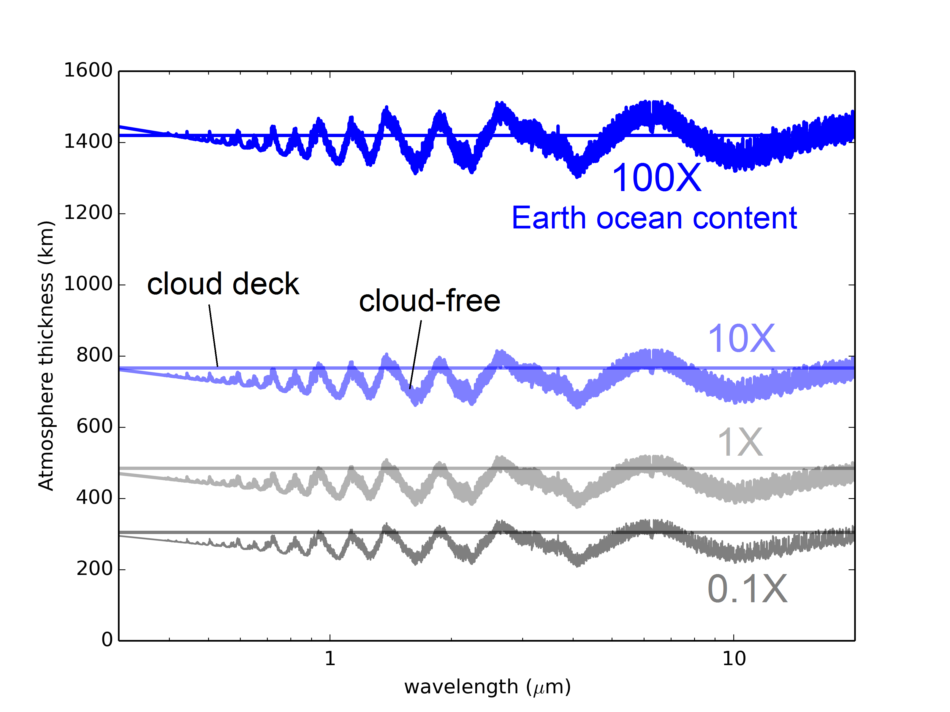
Figure 4: Atmospheric thickness of a post-runaway greenhouse planetary atmosphere as a function of wavelength (from 0.3 to 20 $\mu$m, and for different total water content (from 0.1 to 100$\times$ the Earth ocean content). Atmospheric thickness is plotted for cloudy (horizontal lines) and cloud-free scenarios, for comparison.

Step 5 -

We compute the transit atmospheric thickness of the post-runaway greenhouse atmosphere (as seen during a transit observation) using two endmember approaches:

1. We assume that the transit atmospheric thickness of the atmosphere is defined by the top of the water cloud layer (assumed to be optically thick), that we estimate using the top of the moist convective layer. This approach likely overestimates the transit atmospheric thickness of the atmosphere.

2. We compute the high-resolution wavelength-dependent thickness of the atmosphere (assuming a cloud-free atmosphere) using the line by line radiative transfer model PUMAS, integrated in the Planetary Spectrum Generator (Villanueva et al., 2018). In this approach, the transit radius is mainly controled by H₂O band lines absorption and Rayleigh scattering. This approach likely underestimates the transit atmospheric thickness of the atmosphere.

Figure 4 shows how the transit atmospheric thickness of the post-runaway greenhouse atmosphere varies as a function of wavelength for a cloud-free versus a cloudy atmosphere. Both the cloud-free and cloudy cases give relatively similar transit atmospheric thickness throughout the entire spectrum. This is not really surprising, because the upper atmosphere is cold enough (see Fig. 2) that variations of the optically thick pressure level produce weak atmospheric thickness change (if the temperature is low, the atmospheric scale height is also low).

Figure 5A shows how the atmospheric thickness of a planet in post-runaway greenhouse state $z_{\text{atm, post-runaway}}$ (solid black line) varies as a function of the total water content. When substracting for the thickness of the condensed water layer $z_{\text{water layer}}$ (solid blue line; for present-day Earth, $z_{\text{water layer}}$ = 2.7 km) and the initial atmospheric thickness of a planet in temperate climate state $z_{\text{atm, pre-runaway}}$, this provides the net transit radius change $\Delta R$ resulting from the transition between a temperate to a post-runaway greenhouse climate state, calculated formally as follows:

$$\Delta R\leavevmode\nobreak\ =\leavevmode\nobreak\ z_{\text{atm, post-runaway}}-(z_{\text{atm, pre-runaway}}+z_{\text{water layer}})$$ (1)

For simplicity, and also because the nature of the pre-runaway atmosphere is unknown, we assume in our calculations that $z_{\text{atm, pre-runaway}}$ is equal to 0. This seems a reasonable assumption given that it has been shown that the transit atmospheric thickness of Earth-like atmospheres should not exceed a few tens of kilometers, at least in the visible and infrared spectral domains (Ehrenreich et al., 2006; Kaltenegger & Traub, 2009; Bétrémieux & Kaltenegger, 2013). The thickness of the condensed water layer $z_{\text{water layer}}$ is however accounted for because it can have a significant effect on the calculation of the radius change for the case of large water content (Fig. 5A, blue curve).

The net radius change varies from $\sim$ 300 km (for 0.1$\times$ Earth ocean water content, or 0.002$\%$ of Earth mass) up to $\sim$ 1100 km (for 100 Earth ocean water content or 2$\%$ of Earth mass), and could possibly be even higher for larger water contents, and less massive planets. The larger the water content of the planet, the greater the radius inflation.

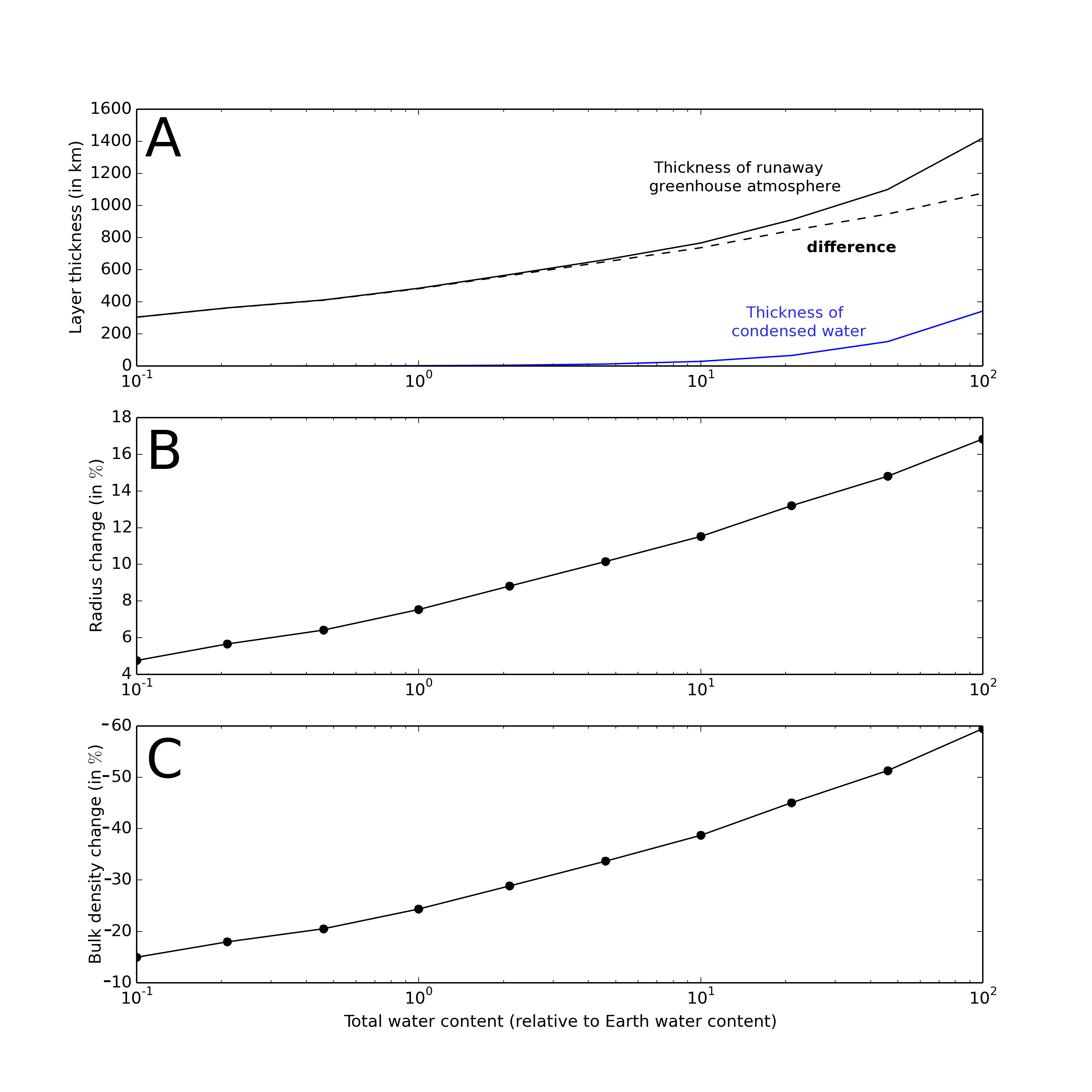
Figure 5: Effect of the total water content on: (A) the thickness of the atmosphere (for a planet in post-runaway greenhouse climate state, in black) and the thickness of a condensed water layer (for a planet in temperate climate state, in blue). The difference has been highlighted in a black, dashed line. (B) the net radius change. (C) the net density change. Net radius (B) and density (C) changes are changes relative to Earth radius and density.

This net absolute radius change can be translated into a net relative radius change (Fig. 5B) and a net relative density change (Fig. 5C), relative to Earth radius and density values. We predict that planets with large water reservoir (at least 2$\%$ of Earth mass or more) would experience – when transitioning from a temperate to a post-runaway greenhouse climate state – a rapid radius increase that could reach or exceed 17$\%$ of Earth radius, and a rapid apparent density drop that could reach or exceed 60$\%$ of Earth density. These radius and density changes could be further amplified by (i) the runaway-greenhouse-induced thermal expansion of the interior (Seager et al., 2007), due to the extreme change of surface temperature boundary condition (from hundreds of Kelvins for a temperate climate planet to thousands of Kelvins for a post-runaway greenhouse planet), as well as by (ii) the change of internal structure and composition. For example, Bower et al. (2019) recently showed that the melting of the mantle (possibly induced by the runaway greenhouse positive feedback) can lead to an additional radius expansion $\sim$ 5$\%$.

Moreover, by modifying the internal structure of the planet, the hot post-runaway greenhouse atmosphere could also modify gas exchanges between the interior and the atmosphere (Ikoma et al., 2018; Bower et al., 2019). These gas exchanges could affect the amount of volatile (e.g. H₂O) outgassing and intake from the interior and thus the calculation of the post-runaway greenhouse planet radius. We leave these calculations for a future study.

The transit net radius change due to the runaway greenhouse transition is orders of magnitude stronger than the spectral variation of the atmospheric thickness due to absorption by H₂O band lines, even in absence of clouds (Fig. 4). This is important because it indicates that the transit photometry measurement of radius variation due to the runaway-greenhouse-induced transition is potentially much easier to do than the transmission spectroscopy measurement of H₂O-induced spectral changes of the transit radius. The latter have been shown to be very difficult to detect, mostly because of clouds (Ehrenreich et al., 2006; Fauchez et al., 2019). Note however that while transmission spectroscopy can be used to identify water in a single planet, here the proposed technique requires to perform transit photometry on multiple planets (see next section).

As long as water remains an important component (in condensed form at the surface, or in the form of vapour in the atmosphere) of the planet, the transition from a temperate state to a post-runaway greenhouse state can in principle occur in both directions, i.e. from temperate to steam atmosphere (Kasting et al., 1993; Kopparapu et al., 2013), but also from steam to temperate atmosphere (Hamano et al., 2013; Lebrun et al., 2013). This indicates that the runaway greenhouse radius inflation (or deflation) effect can theoretically occur around any type of host star, that the brightness of the host star increases (e.g. for Sun-like stars) or decreases (e.g. for M stars, during the extended Pre-Main-Sequence phase) over time.

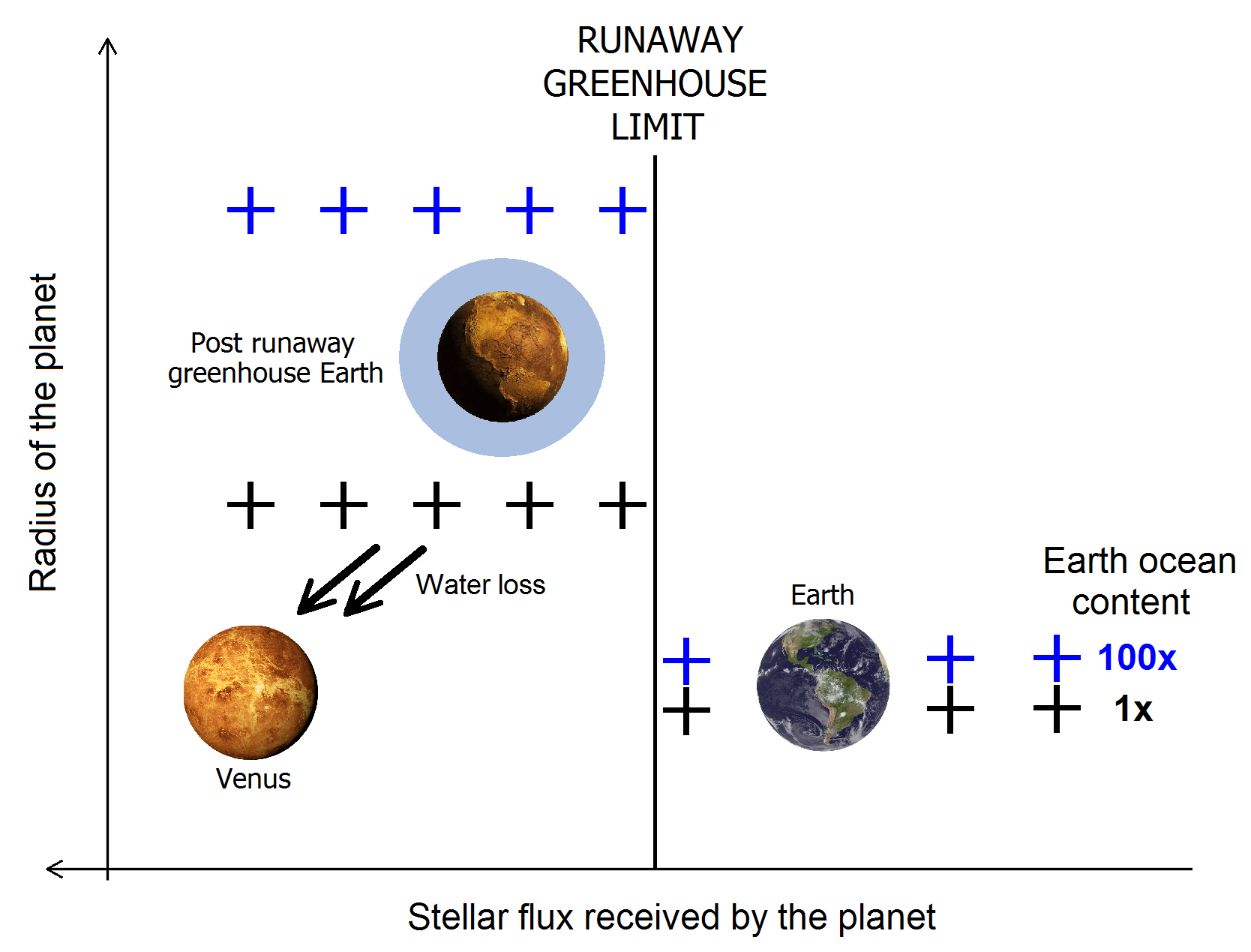
Figure 6: Simplified sketch of the runaway greenhouse radius inflation effect, illustrating how the transit radius of an Earth-like planet varies as a function of stellar irradiation, assuming two different water reservoirs (1 and 100$\times$ the Earth ocean water content). At the runaway greenhouse limit, a planet experiences a sharp transition from a temperate to a post-runaway greenhouse climate (or vice versa). This results in a sharp variation of the radius and density. While efficient atmospheric escape could erase the runaway greenhouse radius inflation effect for planets with limited water reservoir (e.g. Venus), it should have a much less pronounced effect on water-rich planets (e.g. with 100x the Earth ocean content), based on theoretical escape rate estimates (Bolmont et al., 2017).

4 Prospects for an observational test

This runaway greenhouse radius inflation effect could be tested observationally using at least two different approaches.

First, upcoming space missions such as TESS (Ricker et al., 2015), CHEOPS (Benz et al., 2018) and PLATO (Rauer et al., 2014) will provide precise measurements of the radii of numerous Earth-size exoplanets orbiting on both sides of the theoretical runaway greenhouse limit, for M-, K- and potentially even G-type stars. The radius change $\Delta R/R$ between a pre– and post–runaway-greenhouse planet (from Fig. 5B) can be converted into a change of the transit depth, $\Delta(\Delta F/F)=({r_{p}}^{2}(1+\Delta R/R)^{2}-{r_{p}}^{2})/{r_{\star}}^{2}$, where $r_{p}$ and $r_{\star}$ are the planetary and stellar radii, respectively (Winn, 2010). Assuming an Earth-size planet (which has a transit depth in front of a Sun-like star of $\sim$80 ppm), we calculate $\Delta(\Delta F/F)$ for different stellar radii and total water contents of the planet. For G-type stars ($r_{\star}\approx 1\leavevmode\nobreak\ R_{\odot}$), the difference in transit depth between the pre– and post–runaway-greenhouse planet is between 8 and 31 ppm depending on the water content of the planet (between 0.1 and $100\times$ the Earth water content, respectively). This values raises to 17–63 ppm for a K-type star ($r_{\star}\approx 0.7\leavevmode\nobreak\ R_{\odot}$). Red dwarfs offer the largest transit depth differences: an early-type M dwarf ($r_{\star}\approx 0.5\leavevmode\nobreak\ R_{\odot}$) yields transit depth differences in 32–122 ppm, while a late-type, ultracool M dwarf like TRAPPIST-1 ($r_{\star}\approx 0.1\leavevmode\nobreak\ R_{\sun}$) offers transit depth differences in 0.08–0.3% (for water contents in 0.1–$100\times$ the Earth water content, respectively). The CHEOPS space mission (Benz et al., 2018) will have a photometric precision of 20 ppm for bright stars ($6\leq V\leq 9$) and 85 ppm for faint stars ($9<V\leq 12$). It could, in principle, measure such transit depth differences pending habitable-zone, Earth-size exoplanets transiting stars bright enough are known. This is not the case yet. The TESS mission is expected to yield between 20 and 40 Earth-size planets, a handful of which will be found in the habitable zone of M dwarfs (Barclay et al. 2018; see their Fig. 11). These objects, if they are similar to TRAPPIST-1, will likely remain beyond the faint limit of CHEOPS in the optical. However, one could imagine obtaining very precise infrared radii using space telescopes like ARIEL (Tinetti et al., 2018) or the James Webb Space Telescope (Greene et al., 2016). The PLATO mission (Rauer et al., 2014) aims at finding many habitable-zone planets for stars as early as the Sun. The PLATO sample, for which ages will also be determined, might thus represent a good opportunity to detect and constrain the runaway greenhouse radius inflation effect. These radii measurements will be complemented with follow-up precise radial velocity mass measurements using ground-based spectrographs such as ESPRESSO on the VLT (Pepe et al., 2014), CARMENES at Calar Alto Observatory (Quirrenbach et al., 2014) or SPIRou on the CFHT (Artigau et al., 2014). Note that the Kepler/K2 sample lacks terrestrial-size, temperate planets around bright stars (whose mass can be measured by radial velocity). It cannot therefore be used as is to test the runaway greenhouse radius inflation effect.

The abrupt radius inflation – resulting from the runaway-greenhouse-induced transition – should produce an extreme planet density drop that could be detected statistically using a sample of terrestrial-size planets located on both sides of the theoretical inner edge of the Habitable Zone. The detailed calculation to estimate how many planets are needed could be done following a statistical approach (Bean et al., 2017) similar to the detection and characterisation of the gap in the radius distribution due to the transition between rocky and volatile-rich exoplanets (Weiss & Marcy, 2014; Rogers, 2015; Fulton et al., 2017). Selsis et al. (2007a) provides the theoretical framework to evaluate typical sources of uncertainties that need to be accounted for in this statistical calculation. We acknowledge that the process by which a planet goes into the runaway greenhouse positive feedback and inflates its atmosphere has not been studied in time-dependent detail here. Although that time change is likely short, it remains an uncertain parameter that must be marginalized over in any statistical inference based on the target set for the analysis being proposed here. Eventually, the true population (most likely a mix of water-rich and dry planets) will not be known in advance, and the degree to which the dry planets exist in the sample will dilute the measurements. Moreover, the presence of terrestrial-mass planets with a thick H₂/He envelope (Luger et al., 2015; Owen & Mohanty, 2016) could further dilute the measurements. It is not known if such planets exist (i.e. evolved Earth-mass planets with a thick H₂/He envelope) and if so, to what extent they are abundant. However, these planets are potentially easier to characterize with transmission spectroscopy due to their high atmospheric scale height (De Wit et al., 2016; de Wit et al., 2018; Moran et al., 2018). These planets could therefore potentially be identified and removed from the sample. In the end, estimating the minimum number of planets needed to begin to observe the runaway greenhouse radius inflation effect is a very difficult task, as it depends on many unknown parameters, such as the abundance of water in the planet sample, as well as the accuracy of density measurements made with the telescopes and ground-based spectrographs mentioned above. Although the effect could possibly be detected with only a handful of planets if they are all very rich in water (and with no H₂/He envelope), the possible presence of dry planets and/or planets with a H₂/He envelope would dilute the expected signal, which could considerably increase the number of planets needed to identify the effect, possibly to a number far too large to be reached by current and forthcoming telescopes. We encourage future studies to evaluate more precisely the minimum number of planets and the accuracy at which their density should be known in order to confidently detect the runaway greenhouse radius inflation effect, for different water content scenarios.

Secondly, such abrupt density change could be detected locally in multiplanetary systems, such as the TRAPPIST-1 resonant chain (Gillon et al., 2016, 2017; Luger et al., 2017) - when planet masses will be known with good enough precision. TRAPPIST-1 is a particularly interesting case study, because:

• it has been speculated that some of the planets may possess large reservoirs of water (Grimm et al., 2018).

• planets are located on both sides of the theoretical runaway greenhouse limit, which is thought to lie between the orbit of TRAPPIST-1d and TRAPPIST-1e (Kopparapu et al., 2013; Wolf, 2017; Turbet et al., 2018).

The detailed analysis of the impact of the runaway greenhouse radius inflation effect within TRAPPIST-1 is currently the subject of a detailed, separate study (Turbet et al., publication in preparation).

5 Discussions

The detection of such abrupt density change could be used to obtain information on:

1. the concept of runaway greenhouse,

that defines the inner edge of the traditional Habitable Zone (Kasting et al., 1993; Kopparapu et al., 2013). The detection of a sharp transition of planet density (locally or statistically) in the predicted range of instellation (Fig. 6) would indeed validate the concept of runaway greenhouse and Habitable Zone. In particular, the abrupt density change could be used to estimate the limit of the runaway greenhouse transition, possibly as a function of the type of host star. This would make it possible to empirically estimate the position of the inner edge of the Habitable Zone. More importantly, this could provide an empirical measurement of the irradiation at which Earth analogs orbiting a Sun-like star transition to runaway greenhouse. This is especially relevant to the PLATO mission, which aims at detecting Earth-size planets orbiting in the Habitable Zone of Sun-like stars. This astronomical measurement would make it possible to statistically estimate how close Earth is from the runaway greenhouse.

2. the presence (and statistical abundance) of water in temperate, Earth-size exoplanets,

depending on the amplitude of the measured density variation. For a given planet sample (e.g. assuming a given range of host star type), the runaway greenhouse radius inflation effect can only be detected if water has remained abundant on most planets located on both sides of the runaway greenhouse irradiation limit. The ability of planets to retain their water depends on (i) the efficiency of initial water accretion during planetary formation and on (ii) the efficiency of atmospheric escape processes during planetary evolution (Tian & Ida, 2015). The latter is particularly important for post-runaway greenhouse atmospheres for which water is dominant in the upper atmosphere and is exposed to photolysis and thus to important water loss to space (Kasting, 1988). For instance, a steam atmosphere planet (with Earth-like bulk properties) orbiting at the location of the runaway greenhouse limit could experience a water loss as high as a few Earth ocean water content per billion year (Selsis et al., 2007b; Hamano et al., 2015; Bolmont et al., 2017), assuming the energy-limited approximation (Watson et al., 1981). Note that the runaway greenhouse radius inflation could increase the escape rate by a factor of $\sim$ (1.17)³ = 1.6 maximum (Erkaev et al., 2007) for an extreme radius increase of 17$\%$ (for 100$\times$ the Earth water ocean content). As a result, planets that started with an Earth-like water content or lower can lose all their water rather quickly, i.e. in just a few hundred million years. However, both water atmospheric loss and water delivery during planetary formation are highly unconstrained processes. In particular, the initial water content of some temperate, terrestrial-size planets could be as high as hundreds of Earth ocean water content (Raymond et al., 2004; Léger et al., 2004; Tian & Ida, 2015), making atmospheric escape processes inefficient to remove water from water-rich (i.e. substantially richer than the present-day Earth ocean water content) steam planets receiving irradiation not significantly higher than the runaway greenhouse irradiation limit, based on the aforementioned water loss estimates. As a result, planets that started with significantly more water than Earth or that are robust to water loss processes should remain water-rich throughout their entire evolution. They are therefore the ideal type of planets for detecting and characterizing the runaway greenhouse radius inflation effect. In general, if the sampled planets have mainly a water-rich composition, then we predict that the runaway greenhouse radius inflation should be strong. Conversely, if the sampled planets are mainly dry (e.g. because they have lost all their water due to atmospheric escape ; possibly as in the Solar System, with Venus for which efficient atmospheric escape has likely swept almost all of the initial water reservoir) then the predicted radius inflation should be absent in the sampled population. Even a non-detection of the runaway greenhouse radius inflation effect could therefore be used to obtain constraints on (i) the maximum water content of the sampled population of temperate Earth-size planets, as well as (ii) on the minimal efficiency of atmospheric escape processes (Fig. 6). We acknowledge these two constraints (i) and (ii) are degenerate and a detailed analysis would be needed to estimate these parameters and their uncertainties.

Appendix A The 1D LMD Generic inverse climate model

Our 1D version of the LMD Generic model is a single-column inverse radiative-convective climate model following the same approach (’inverse modeling’) as in Kasting et al. (1984); Kopparapu et al. (2013); Turbet et al. (2019). The atmosphere is decomposed into 200 logarithmically-spaced layers that extend from the ground to the top of the atmosphere arbitrarily fixed at 0.1 Pascal. The atmosphere, assumed here to be composed of 1 bar of N₂ and a variable amount of H₂O, is divided in at most three physical layers constructed as in Marcq (2012); Marcq et al. (2017); Pluriel et al. (2019). From the surface to the top, the atmosphere is composed of:

1. an unsaturated troposphere, where heat transport is dominated by dry convection. The mixing ratio H₂O/N₂ is constant in this layer.

2. a moist troposphere, saturated in water vapour, where heat transport is dominated by moist convection. It is in this layer that clouds are expected to form.

3. a purely radiative, isothermal mesosphere with a temperature fixed to 200 K as previously done for similar applications (Kasting 1988; Kopparapu et al. 2013; Leconte et al. 2013; Marcq et al. 2017) (i.e. a water-rich mesosphere), which have shown that even for very hot surface temperatures, these atmospheres exhibit rather cool temperatures at their top. In this layer, the mixing ratio H₂O/N₂ is constant.

The moist troposphere is present only if the saturation of water vapor is reached at any altitude. If this occurs at the surface, then it is the unsaturated troposphere that does not exist.

The dry and moist convective layers are constructed using Kasting (1988) formulation of the lapse rate, and as done in Marcq et al. (2017). While N₂ is assumed to behave like an ideal gas, the non-ideal behaviour of H₂O is accounted by using the Fortan NBS/NRC steam tables (Haar et al. 1984), as in Marcq et al. (2017). Comparisons with the IAPWS-95 steam tables (Wagner & Pruß 2002) gave negligible differences on the thermal profiles, at least for the range of applications explored in this work.

Once the thermal profile of the atmosphere is constructed, we compute the radiative transfer in both visible and thermal infrared spectral domains, and through the 200 atmospheric layers, using the radiative transfer of the LMD Generic Model, historically based on the NASA Ames radiation code (https://spacescience.arc.nasa.gov/mars-climate-modeling-group/models.html). The radiative transfer calculations are performed on 38 spectral bands in the thermal infrared and 36 in the visible domain, using the ’correlated-k’ approach (Fu & Liou 1992), as in Leconte et al. (2013). 16 non-regularly spaced grid points were used for the g-space integration, where g is the cumulative distribution function of the absorption for each band. Absorption coefficients are exactly the same than those used in Leconte et al. (2013), and were designed for H₂O-dominated atmospheres as expected for planets experiencing a runaway greenhouse transition. For the radiative transfer calculations, the Sun (assumed to be the host star) is assumed to remain fixed, at a zenith angle of 60^∘. The surface albedo is arbitrarily fixed to 0.2.

From the radiative transfer calculations, we can derive (1) the Outgoing Longwave Radiation (OLR) and (2) the planetary albedo $A_{p}$. The effective flux S${}_{\text{eff}}$ can then be computed as $\frac{OLR}{(1-A_{p})\leavevmode\nobreak\ F_{\oplus}}$, with $F_{\oplus}$ the average insolation at the top of the atmosphere on Earth, equal to one fourth of the solar constant, i.e. 340.5 W m^-2. The effective flux can be interpreted as the stellar flux (relative to the solar flux received by Earth today) necessary for a planet to be in radiative equilibrium, given the OLR of the planet is known.