DiCENet: Dimension-wise Convolutions for Efficient Networks

Sachin Mehta, Hannaneh Hajishirzi, and Mohammad Rastegari S. Mehta, H. Hajishirzi, and M. Rastegari are with the University of Washington, Seattle, WA, 98195.
E-mail: {sacmehta, hannaneh, mrast}@cs.washington.edu

Abstract

We introduce a novel and generic convolutional unit, DiCE unit, that is built using dimension-wise convolutions and dimension-wise fusion. The dimension-wise convolutions apply light-weight convolutional filtering across each dimension of the input tensor while dimension-wise fusion efficiently combines these dimension-wise representations; allowing the DiCE unit to efficiently encode spatial and channel-wise information contained in the input tensor. The DiCE unit is simple and can be seamlessly integrated with any architecture to improve its efficiency and performance. Compared to depth-wise separable convolutions, the DiCE unit shows significant improvements across different architectures. When DiCE units are stacked to build the DiCENet model, we observe significant improvements over state-of-the-art models across various computer vision tasks including image classification, object detection, and semantic segmentation. On the ImageNet dataset, the DiCENet delivers 2-4% higher accuracy than state-of-the-art manually designed models (e.g., MobileNetv2 and ShuffleNetv2). Also, DiCENet generalizes better to tasks (e.g., object detection) that are often used in resource-constrained devices in comparison to state-of-the-art separable convolution-based efficient networks, including neural search-based methods (e.g., MobileNetv3 and MixNet).

Index Terms:

Convolutional Neural Network, Image Classification, Object Detection, Semantic Segmentation, Efficient Networks.

1 Introduction

The basic building layer at the heart of convolutional neural networks (CNNs) is a convolutional layer that encodes spatial and channel-wise information simultaneously [1, 2, 3]. Learning representations using this layer is computationally expensive. Improving the efficiency of CNN architectures as well as convolutional layers is an active area of research. Most recent attempts have focused on improving the efficiency of CNN architectures using compression- and quantization-based methods (e.g. [4, 5]). Recently, several factorization-based methods have been proposed to improve the efficiency of standard convolutional layers (e.g. [6, 7, 8]). In particular, depth-wise separable convolutions [7, 9] have gained a lot of attention (see Figure 1(a)). These convolutions have been used in several efficient state-of-the-art architectures, including neural search-based architectures [10, 11, 12, 13].

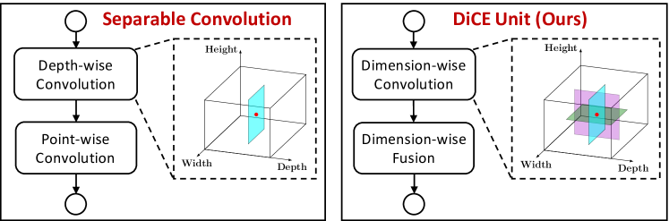
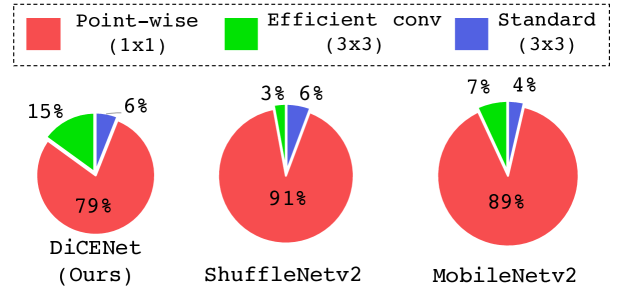
Refer to caption — (a) Block of separable convolutions and the DiCE unit. Convolutional kernels are highlighted in color (depth-, width-, and height-wise).

Separable convolutions factorize the standard convolutional layer in two steps: (1) a light-weight convolutional filter is applied to each input channel using depth-wise convolutions [9] to learn spatial representations, and (2) a point-wise ( $1\times 1$ ) convolution is applied to learn linear combinations between spatial representations. Though depth-wise convolutions are efficient, they do not encode channel-wise relationships. Therefore, separable convolutions rely on point-wise convolutions to encode channel-wise relationships. This puts a significant computational load on point-wise convolutions and makes them a computational bottleneck. For example, point-wise convolutions account for about 90% of total operations in ShuffleNetv2 [16] and MobileNetv2 [10].

In this paper, we introduce DiCENet, Dimension-wise Convolutions for Efficient Networks that encodes spatial and channel-wise representations efficiently. Our main contribution is the novel and generic module, the DiCE unit (Figure 1(a)), that is built using Dimension-wise Convolutions (DimConv) and Dimension-wise Fusion (DimFuse). The DimConv applies a light-weight convolutional filter across “each dimension” of the input tensor to learn local dimension-wise representations while DimFuse efficiently combines these dimension-wise representations to incorporate global information.

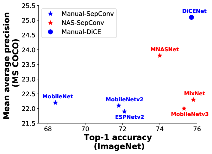
With DimConv and DimFuse, we build an efficient convolutional unit, the DiCE unit, that can be easily integrated into existing or new CNN architectures to improve their performance and efficiency. Figure 1 shows that the DiCE unit is effective in comparison to widely-used separable convolutions. Compared to state-of-the-art manually designed networks (e.g., MobileNet [7], MobileNetv2 [10], and ShuffleNetv2 [16]), DiCENet delivers significantly better performance. For example, for a network with about 300 million floating point operations (FLOPs), DiCENet is about 4% more accurate than MobileNetv2. Importantly, DiCENet, a manually designed network, delivers similar or better performance than neural architecture search (NAS) based methods. For example, DiCENet is 1.7% more accurate than MNASNet for a network with about 300 MFLOPs.

We empirically demonstrate in Section 6 and Section 7 that the DiCENet network, built by stacking DiCE units, achieves significant improvements on standard benchmarks across different tasks over existing networks. Compared to existing efficient networks, DiCENet generalizes better to tasks (e.g., object detection) that are often used in resource-constrained devices. For instance, DiCENet achieves about 3% higher mean average precision than MobileNetv3 [14] and MixNet [15] on the MS-COCO object detection task with SSD [17] as a detection pipeline (Fig. 1(b)). Our source code in PyTorch is open-source and is available at https://github.com/sacmehta/EdgeNets/.

2 Related Work

CNN architecture designs: Recent success in visual recognition tasks, including classification, detection, and segmentation, can be attributed to the exploration of different CNN designs (e.g., [1, 2, 3, 7]). The basic building layer in these networks is a standard convolutional layer, which is computationally expensive. Factorization-based methods improve the efficiency of these layers. For instance, flattened convolutions [6] approximate a standard convolutional layer with three point-wise convolutions that are applied sequentially, one point-wise convolution per tensor dimension. These convolutions ignore spatial relationships between pixels and do not generalize across a wide variety of computer vision tasks (e.g., detection and segmentation) and large scale datasets (e.g., ImageNet and MS-COCO). To improve the efficiency of standard convolutions while maintaining the performance and generalization ability at scale, depth-wise separable convolutions [7] are proposed that factorizes the standard convolutional layer into depth-wise and point-wise convolution layers. Most of the efficient CNN architectures are built using these separable convolutions, including MobileNets [7, 10], ShuffleNets [18, 16], and ESPNetv2 [11]. In this work, we introduce dimension-wise convolutions that generalize depth-wise convolutions to all dimensions of the input tensor. We also introduce an efficient way for combining these dimension-wise representations. As confirmed by our experiments in Section 5, 6 and 7, the DiCE unit is more effective than separable convolutions.

Neural architecture search: Recently, neural architecture search-based methods have been proposed to automatically construct network architectures (e.g., [19, 13, 20, 12, 14]). These methods search over a large network space (e.g., MNASNet [12] searches over 8K different design choices) using a dictionary of pre-defined search space parameters, including different types of convolutional layers and kernel sizes, to find a heterogeneous network structure that satisfies optimization constraints, such as inference time. The proposed unit is novel and cannot be discovered using existing neural search-based methods (e.g., [12, 13, 21]). However, we believe that better neural architectures can be discovered by adding the DiCE unit in neural search dictionary.

Quantization, compression, and distillation: Network quantization-based approaches [22, 23, 24, 25] approximate 32-bit full precision convolution operations with fewer bits. This improves inference speed and reduces the amount of memory required for storing network weights. Network compression-based approaches [26, 27, 4, 28, 5] improve the efficiency of a network by removing redundant weights and connections. Unlike network quantization and compression, distillation-based approaches [29, 30, 31] improve the accuracy of (usually shallow) networks by supervising the training with large pre-trained networks. These approaches are effective for improving the efficiency of a network, including efficient architecture designs (e.g., [32, 33]) and are orthogonal to our work. We believe that the efficiency of DiCENet can be further improved using these methods.

3 DiCENet

Standard convolutions encode spatial and channel-wise information simultaneously, but they are computationally expensive. To improve the efficiency of standard convolutions, separable (or depth-wise separable) convolutions are introduced [7], where spatial and channel-wise information is encoded separately using depth-wise and point-wise convolutions, respectively. Though this factorization is effective, it puts a significant computational load on point-wise convolutions and makes them a computational bottleneck (see Figure 2).

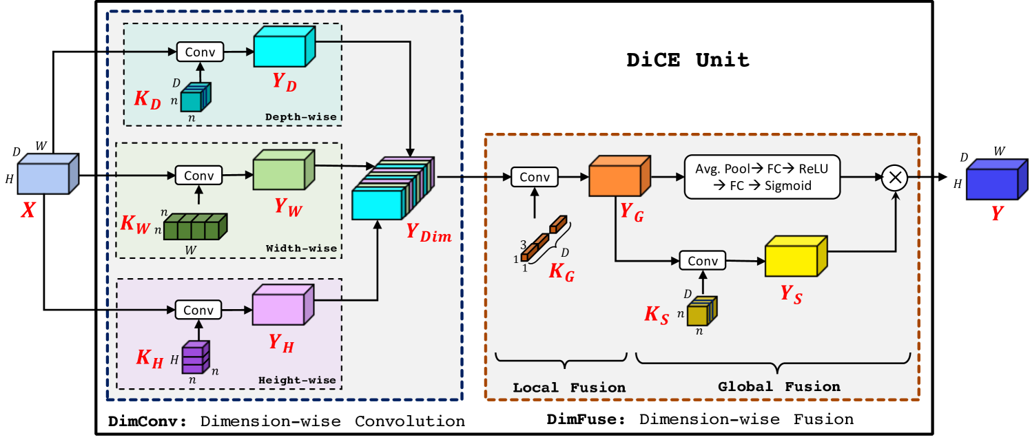
To encode spatial and channel-wise information efficiently, we introduce the DiCE unit and is shown in Figure 3. The DiCE unit factorizes standard convolution using Dimension-wise Convolution (DimConv, Section 3.1) and Dimension-wise Fusion (DimFuse, Section 3.2). DimConv applies a light-weight filtering across each dimension of the input tensor to learn local dimension-wise representations. DimFuse efficiently combines these representations from different dimensions and incorporates global information. The ability to encode local spatial and channel-wise information from all dimensions using DimConv enables the DiCE unit to use DimFuse instead of computationally expensive point-wise convolutions.

3.1 Dimension-wise Convolution (DimConv)

We use dimension-wise convolutions (DimConv) to encode depth-, width-, and height-wise information independently. To achieve this, DimConv extends depth-wise convolutions to all dimensions of the input tensor $\mathbf{X}\in\mathbb{R}^{D\times H\times W}$ , where $W$ , $H$ , and $D$ corresponds to width, height, and depth of $\mathbf{X}$ . As illustrated in Figure 3, DimConv has three branches, one branch per dimension. These branches apply $D$ depth-wise convolutional kernels $\mathbf{k}_{D}\in\mathbb{R}^{1\times n\times n}$ along depth, $W$ width-wise convolutional kernels $\mathbf{k}_{W}\in\mathbb{R}^{n\times n\times 1}$ along width, and $H$ height-wise convolutional kernels $\mathbf{k}_{H}\in\mathbb{R}^{n\times 1\times n}$ kernels along height to produce outputs $\mathbf{Y_{D}}$ , $\mathbf{Y_{W}}$ , and $\mathbf{Y_{H}}\in\mathbb{R}^{D\times H\times W}$ that encode information from all dimensions of the input tensor. The outputs of these independent branches are concatenated along the depth dimension, such that the first spatial plane of $\mathbf{Y_{D}}$ , $\mathbf{Y_{W}}$ , and $\mathbf{Y_{H}}$ are put together and so on, to produce the output $\mathbf{Y_{Dim}}=\{\mathbf{Y_{D}},\mathbf{Y_{W}},\mathbf{Y_{H}}\}\in\mathbb{R}^{3D\times H\times W}$ .

3.2 Dimension-wise Fusion (DimFuse)

The dimension-wise convolutions encode local information from different dimensions of the input tensor, but do not capture global information. A standard approach to combine features globally in CNNs is to use a point-wise convolution [3, 7]. A point-wise convolutional layer applies $D$ point-wise kernels $\mathbf{k}_{p}\in\mathbb{R}^{3D\times 1\times 1}$ and performs $3D^{2}HW$ operations to combine dimension-wise representations of $\mathbf{Y_{Dim}}\in\mathbb{R}^{3D\times H\times W}$ and produce an output $\mathbf{Y}\in\mathbb{R}^{D\times H\times W}$ . This is computationally expensive. Given the ability of DimConv to encode spatial and channel-wise information (though independently), we introduce a fusion module, Dimension-wise fusion (DimFuse), that allows us to combine representations of $\mathbf{Y_{Dim}}$ efficiently. As illustrated in Figure 3, DimFuse factorizes the point-wise convolution in two steps: (1) local fusion and (2) global fusion.

$\mathbf{Y_{Dim}}\in\mathbb{R}^{3D\times H\times W}$ concatenates spatial planes along depth dimension from $\mathbf{Y_{D}}$ , $\mathbf{Y_{W}}$ , and $\mathbf{Y_{H}}$ (see Figure 3). Therefore, $\mathbf{Y_{Dim}}$ can be viewed as a tensor with $D$ groups, each group with three spatial planes (one from each dimension). DimFuse uses a group point-wise convolutional layer to combine dimension-wise information contained in $\mathbf{Y_{Dim}}$ . In particular, this group convolutional layer applies $D$ point-wise convolutional kernels $\mathbf{k}_{G}\in\mathbb{R}^{3\times 1\times 1}$ to $\mathbf{Y_{Dim}}$ and produces an output $\mathbf{Y_{G}}\in\mathbb{R}^{D\times H\times W}$ . Since $D$ kernels in $\mathbf{k}_{G}$ operates independently on $D$ groups in $\mathbf{Y_{Dim}}$ , we call this local fusion operation.

To efficiently encode the global information in $\mathbf{Y_{G}}$ , DimFuse learns spatial and channel-wise representations independently and then propagate channel-wise encodings to spatial encodings using an element-wise multiplication. Specifically, DimFuse encodes spatial representations by applying $D$ depth-wise convolutional kernels $\mathbf{k}_{S}\in\mathbb{R}^{1\times n\times n}$ to $\mathbf{Y_{G}}$ to produce an output $\mathbf{Y}_{S}$ .¹¹1When the depth of $\mathbf{Y_{Dim}}$ is different from $\mathbf{Y}$ , then $\mathbf{k}_{S}$ is a group convolution, where number of groups is the greatest common divisor between the depth of $\mathbf{Y_{Dim}}$ and $\mathbf{Y}$ . Motivated by Squeeze-Excitation (SE) unit [34], we squeeze spatial dimensions of $\mathbf{Y_{G}}$ and encode channel-wise representations using two fully connected (FC) layers. The first FC layer reduces the input dimension from $D$ to $\frac{D}{4}$ while the second FC layer expands dimensionality from $\frac{D}{4}$ to $D$ . To allow these fully connected layers to learn non-linear representations, a ReLU activation is added in between these two layers. Similar to the SE unit, spatial representations $\mathbf{Y_{G}}$ are then scaled using these channel-wise representations to produce output $\mathbf{Y}$ .

The computational cost of DimFuse is $HWD(3+n^{2}+D)$ . Effectively, DimFuse reduces the computational cost of point-wise convolutions by a factor of $\frac{3D}{3+n^{2}+D}$ . DimFuse uses $n=3$ , so the computational cost is approximately $3\times$ smaller than that of the point-wise convolution.

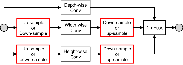
3.3 DiCE Unit for Arbitrary Sized Inputs

The DiCE unit stacks DimConv and DimFuse to encode spatial and channel-wise information in the input tensor efficiently. However, the two kernels (i.e., $\mathbf{k}_{H}$ and $\mathbf{k}_{W}$ ) in DimConv unit correspond to spatial dimensions of the input tensor. This may pose a challenge when spatial dimensions of the input tensor are different from the ones with which the network is trained. To make DiCE units invariant to spatial dimensions of the input tensor, we dynamically scale (either up-sample or down-sample) the height or width dimension of the input tensor to the height or width of the input tensor used in the pretrained network. The resultant tensors are then scaled (either down-sampled or up-sampled) back to their original size before being fed to DimFuse; this makes the DiCE unit invariant to input tensor size. Figure 5 sketches the DiCE unit with dynamic scaling. Results in Section 7, especially object detection and semantic segmentation, show that the DiCE unit can handle arbitrary sized inputs.

3.4 DiCENet Architecture

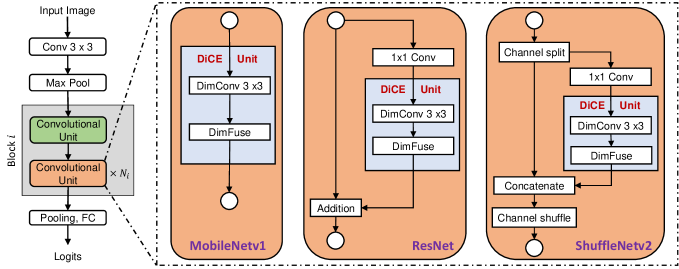
DiCE units are generic and can be easily integrated in any existing network. Figure 4 visualizes the DiCE unit with different architectures: (1) MobileNet [7] stacks separable convolutions (depth-wise convolution followed by point-wise convolution) to learn representations. (2) ResNet [3] introduces the bottleneck unit with residual connections to train very deep networks. The bottleneck unit is a stack of three convolutional layers: one $3\times 3$ depth-wise convolutional layer²²2Our focus is on efficient network. Therefore, we replace standard convolutional layer with depth-wise convolutional layer. surrounded by two point-wise convolutions. This block can be viewed as a point-wise convolution followed by separable convolution. (3) ShuffleNetv2 [16] is a state-of-the-art efficient network that outperforms other efficient networks, including MobileNetv2 [10]. ShuffleNetv2’s unit stacks a point-wise convolution and separable convolution. It also uses channel split and shuffle to promote feature reuse.

To illustrate the performance benefits and generic nature of the DiCE unit over separable convolutions, we replace separable convolutions with the DiCE unit in these architectures. Our empirical results in Section 5 shows that the DiCE unit with ShuffleNetv2’s architecture delivers the best performance. Therefore, we choose the ShuffleNetv2 [16] architecture and call the resultant network DiCENet (ShuffleNetv2 with the DiCE unit).

CUDA Implementation: DimConv applies $D$ , $W$ , and $H$ depth-wise, width-wise and height-wise convolutional kernels to the input tensor $\mathbf{X}$ to aggregate information from different dimensions of the tensor, respectively. A standard solution would be to apply each kernel independently to the tensor and then concatenate their results, as shown in Figure 7(a). Another solution would be to apply all kernels simultaneously, as shown in Figure 7(b). Compared to three CUDA kernel calls in the former solution, the later one requires one kernel call, thus reducing the kernel launch time. Also, each thread in the CUDA kernel process $3n^{2}$ elements compared to $n^{2}$ elements in the former solution for $n\times n$ convolutional kernels. This maximizes the work done per thread and improves speed. Our results in Section 6 shows that DiCENet is accurate and fast compared to state-of-the-art methods, including neural search-based methods.

(a) Unoptimized (Left to right: depth-wise, height-wise, and width-wise)

(b) Optimized

Figure 7: Implementation of dimension-wise convolution (DimConv). In (a), each kernel is applied to a pixel (represented by red dot) independently. In (b), all kernels are applied to a pixel simultaneously, allowing us to aggregate the information from tensor efficiently. Convolutional kernels are highlighted in color (depth-, width-, and height-wise).

4 Experimental Set-up

Following most architecture designs (e.g. [3, 7, 11]), we evaluate the generic nature of the DiCE unit on the ImageNet dataset in Section 5. We integrate the DiCE unit in different image classification architectures (Figure 4) and study the impact on efficiency and accuracy. We also study the importance of the two main components of the DiCE unit, i.e. DimConv and DimFuse, and show that DiCE units are more effective than separable convolutions [7]. In Section 6, we evaluate the image classification performance of DiCENet on the ImageNet dataset and show that DiCENet delivers similar or better performance than state-of-the-art efficient networks, including neural search-based methods. In Section 7, we evaluate task-level generalization ability of DiCENet on three different visual recognition tasks, i.e. object detection, semantic segmentation, and multi-object classification, that are often used in resource-constrained devices. We demonstrate that DiCENet generalizes better than existing efficient networks that are built using separable convolutions.

Datasets: We use following datasets in our experiments.

Image classification: For single label image classification, we use ImageNet-1K classification dataset [35]. This dataset consists of 1.28M training and 50K validation images. All networks on this dataset are trained from scratch. For multi-label classification, we use MS-COCO dataset [36] that has 2.9 labels (on an average) per image. We use the same training and validation splits as in [11].

Object detection: We use MS-COCO [36] and PASCAL VOC 2007 [37] datasets for evaluating on the task of object detection. Following a standard convention for training on PASCAL VOC 2007 dataset, we augment it with PASCAL VOC 2012 [38] and PASCAL VOC 2007 trainval set for training and evaluate the performance on PASCAL VOC 2007 test set.

Semantic segmentation: We use PASCAL VOC 2012 [38] dataset for this task. Following a standard convention, we use additional images for training from [39] and [36]. Similar to MobileNetv2 [10], we evaluate the performance on the validation set.

Efficiency metric: We measure efficiency in terms of the number of floating point operations (FLOPs) and inference time. We use PyTorch for training our networks.

5 Evaluating DiCE Unit on ImageNet

We first evaluate the two important properties of the DiCE unit, i.e. generic and efficiency, in Section 5.1. To evaluate this, we replace separable convolutions [7] in different architectures with the DiCE unit (Figure 4). We then study the importance of each component of the DiCE unit, DimConv and DimFuse, in Section 5.2. Recent studies (e.g., MobileNetv3 [14] and MNASNet [12]) uses several different methods, such as exponential moving average (EMA) and large batch sizes, to improve the performance. In Section 5.3, we study the effect of these methods on the performance of DiCENet.

In these experiment, we use the ImageNet dataset [35]. In Section 5.1 and Section 5.2, we follow the experimental setup of ESPNetv2 [11] and ShuffleNetv2 [16] (fewer training epochs with smaller batch size) while in Section 5.3, we follow experimental set-up similar to MobileNets [10, 14] (longer training with larger batch size).

5.1 DiCE Unit vs. Separable Convolutions

Table I shows the performance of the DiCE unit with different architectures at different FLOP ranges. When separable convolutions are replaced with the DiCE unit in MobileNet architecture, we observe significant gains in performance both in terms of accuracy and efficiency. Since this architecture does not employ any advanced methods (e.g., residual connections and channel shuffle) to improve performance, it allows us to understand the “true” gains of the DiCE unit over separable convolutions.

When we replace separable convolutions with the DiCE unit in ResNet and ShuffleNetv2, we observe significant improvements especially for small-(25-60 MFLOPs) and medium-sized (120-170 MFLOPs) models. For instance, the DiCE unit improved the performance of ShuffleNetv2 by about 3% for small-sized model (about 40 MFLOPs). Similarly, ShuffleNetv2 with the DiCE unit requires 24 million fewer FLOPs to achieve the same accuracy as with separable convolutions for medium-sized model (120-170 MFLOPs). These results suggests that the DiCE unit is generic and learns better representations than separable convolutions.

FLOP	Separable conv		DiCE unit		Absolute difference
Range	(SC)		(DU)		(DU - SC)
(in millions)	Top-1	FLOPs	Top-1	FLOPs	Top-1	FLOPs
MobileNet [7]
25-60	49.80	41 M	52.55	29 M	+2.75	-12 M
120-170	65.30	162 M	69.05	167 M	+3.75	+5 M
270-320	68.40	317 M	70.83	277 M	+2.43	-40 M
ResNet [3]
25-60	59.30	59 M	61.35	52 M	+2.05	-7 M
120-170	67.80	142 M	67.90	122 M	+0.10	-20 M
270-320	70.67	302 M	71.80	300 M	+1.13	-2 M
ShuffleNetv2 [16]
25-60	59.69	41 M	62.80	46 M	+3.11	+5 M
120-170	68.14	146 M	68.21	122 M	+0.07	-24 M
270-320	71.80	292 M	72.90	298 M	+1.10	+6 M

TABLE I: Comparison between the DiCE unit and separable convolutions on the ImageNet dataset across different architectures. Models with the DiCE unit requires fewer channels compared to models with separable convolution in order to obtain similar performance. Thus, models with the DiCE unit has fewer FLOPs compared to separable convolutions.

5.2 Importance of DimConv and DimFuse

To understand the significance of each component of the DiCE unit, we replace DimConv with depth-wise convolution and DimFuse with different fusion methods, including point-wise convolutions and squeeze-excitation (SE) unit [34] and study their combinations for two architectures (ResNet and ShuffleNetv2)³³3MobileNet’s performance is significantly lower than ResNet and ShuffleNetv2, therefore, we do not use MobileNet for these experiments.. In these experiments, we study efficient models by restricting the computational budget between 120 and 150 MFLOPs.

Importance of DimConv: We replace depth-wise convolutional layers with DimConv in ResNet and ShuffleNetv2 architectures. Table II(a) shows that these networks with DimConv require about 10-11 million fewer FLOPs to achieve similar accuracy as the depth-wise convolution. These results suggest that encoding spatial and channel-wise information independently in DimConv helps learning better representations compared to encoding only spatial information in depth-wise convolution.

Importance of DimFuse: To understand the effect of DimFuse, we replace DimFuse with two widely used fusion operations, i.e., point-wise convolution and SE unit. Table II(b) summarizes the results. Compared to the widely used combination of depth-wise and point-wise convolutions (or separable convolution), the combination of DimConv and DimFuse (or the DiCE unit) is the most effective and improves the efficiency of networks by 15-20% with little or no impact on accuracy.

The combination of depth-wise and DimFuse is not as effective as DimConv and DimFuse. DimConv encodes local spatial and channel-wise information, which enables the DiCE unit to use a less complex fusion method (DimFuse) for encoding global information. Unlike DimConv, depth-wise convolutions only encode local spatial information and require computationally expensive point-wise convolutions to encode global information.

When point-wise convolutions are replaced with SE unit, the performance of networks with depth-wise and DimConv convolutions dropped significantly. This is because SE unit relies on an existing convolutional unit, such as ResNext [40], to encode global spatial and channel-wise information. When SE unit is used as a replacement for point-wise convolutions, it fails to effectively encode this information; resulting in significant performance drop.

	ResNet		ShuffleNetv2
Layer	FLOPs	Top-1	FLOPs	Top-1
DWise + Point-wise	142 M	67.80	146 M	68.14
DimConv + Point-wise	132 M	68.10	135 M	68.45

(a) Importance of DimConv. DWise denotes depth-wise conv.

	ResNet		ShuffleNetv2
Layer	FLOPs	Top-1	FLOPs	Top-1
DWise + Point-wise (Separable)	142 M	67.80	146 M	68.14
DWise + SE	137 M	63.90	140 M	64.70
DWise + Point-wise + SE	142 M	68.20	146 M	68.60
DWise + DimFuse	136 M	65.90	139 M	66.80
DimConv + Point-wise	132 M	68.10	135 M	68.45
DimConv + SE	134 M	64.80	138 M	65.40
DimConv + Point-wise + SE	132 M	67.90	135 M	68.30
DimConv + DimFuse (DiCE unit)	122 M	67.90	122 M	68.21

(b) Importance of DimFuse. DWise denotes depth-wise conv.

TABLE II: Evaluating DiCE unit on the ImageNet dataset. Top-1 accuracy is reported on the validation set. Models with DiCE unit requires fewer channels compared to models with separable convolution in order to obtain similar performance. Therefore, models with DiCE unit has fewer FLOPs compared to separable convolutions.

Row		Network	ResNet		ShuffleNetv2
#	Layer	Width	FLOPs	Top-1	FLOPs	Top-1
R1	Point-wise + DWise + DimFuse	$1\times$	136 M	65.90	139 M	66.80
R2	DimFuse + DWise + DimFuse	$1\times$	78 M	60.10	78 M	61.80
R3	DimFuse + DWise + DimFuse	$4\times$	141 M	66.20	140 M	66.90
R4	Point-wise + DimConv + DimFuse	$1\times$	122 M	67.90	122 M	68.21
R5	DimFuse + DimConv + DimFuse	$1\times$	72 M	62.10	72 M	63.70
R6	DimFuse + DimConv + DimFuse	$4\times$	129 M	68.20	132 M	69.20

TABLE III: Impact of replacing all pointwise convolutions with DimFuse. Here, DWise denotes depth-wise convolution.

Network	Type	FLOP ranges (in millions)
Network	Type	$<$ 10 M	10-20 M	21-60 M	61-90 M	91-130 M	131-170 M	200 -320 M
MobileNet [7]	Manual		41.5 (14)	56.3 (49)	59.1 (77)	61.7 (110)	65.3 (162)	68.4 (317)
MobileNetv2 [10]	Manual		45.5 (11)	61.0 (50)	63.9 (71)	66.4 (107)	68.7 (153)	71.8 (300)
ESPNetv2 [11]	Manual				66.1 (86)	67.9 (124)		72.1 (284)
CondenseNet [41]	Manual							71.0 (274)
ShuffleNetv2 [16]	Manual	39.1 (8.0)		59.7 (41)			68.1 (142)	71.8 (292)
MNASNet [12]	NAS				62.4 (76)	67.3 (103)		74.0 (317)
FBNet [13]	NAS				65.3 (72)	67.0 (92)		74.1 (295)
MobileNetv3 [14]	NAS				67.4 (66)			75.2 (219)
MixNet [15]	NAS							75.8 (256)
DiCENet-E150-B512 (Ours)	Manual	40.6 (6.5)	46.2 (14)	62.8 (46)	66.5 (70)	67.8 (98)	69.5 (139)	72.9 (298)
DiCENet-E300-B2048 (Ours)	Manual	43.1 (6.5)	48.2 (14)	65.1 (46)	68.5 (70)	69.3 (98)	72.0 (139)	75.7 (298)

TABLE IV: Results on the ImageNet dataset. DiCENet delivers similar or better performance than state-of-the-art methods, including neural architecture search (NAS)-based methods. Here, each entry is represented as top-1 accuracy and FLOPs within parentheses. DiCENet-E150-B512 models are trained for 150 epochs with a batch size of 512 (without EMA and label smoothing) while DiCENet-E300-B2048 models are trained for 300 epochs with an effective batch size of 2048 (with EMA and label smoothing).

	Network statistics			Device: GTX-960 M (Memory = 4GB)		Device: GTX-1080 Ti (Memory = 11 GB)
Model	# Params	# FLOPs	Top-1 Accuracy	Batch size = 1	Batch size = 32	Batch size = 1	Batch size = 32	Batch size = 64
MobileNetv2	3.5 M	300 M	71.8	5.6 $\pm$ 0.2 ms	114 $\pm$ 0.1 ms	5.9 $\pm$ 0.1 ms	22.8 $\pm$ 0.1 ms	44.3 $\pm$ 0.8 ms
ShuffleNetv2	3.5 M	300 M	71.8	5.8 $\pm$ 0.2 ms	80.7 $\pm$ 0.6 ms	5.8 $\pm$ 0.2 ms	12.9 $\pm$ 0.1 ms	24.1 $\pm$ 0.4 ms
MobileNetv3	5.5 M	220 M	75.2	8.5 $\pm$ 0.2 ms	Out-of-memory	9.0 $\pm$ 0.3 ms	20.9 $\pm$ 0.1 ms	40.2 $\pm$ 0.2 ms
DiCENet (Ours)	5.1 M	297 M	75.7	5.9 $\pm$ 0.1 ms	79 $\pm$ 0.1 ms	5.7 $\pm$ 0.1 ms	12.8 $\pm$ 0.1 ms	24.1 $\pm$ 0.6 ms

TABLE V: Inference speed. DiCENet and ShuffleNetv2 are comparatively faster than MobileNetv2 and MobileNetv3 on both devices (Mobile GPU: GTX-960M and Desktop GPU: GTX-1080 Ti). Inference results are an average over 100 trials for RGB input images of size

224\times 224

. We used PyTorch with CUDA 10.2 for measuring speed. MobileNetv2 and ShuffleNetv2 implementations are taken from official PyTorch repository while MobileNetv3’s implementation is taken from [42]. Since efficient implementations of EESP module in ESPNetv2 and mixed depth-wise convolution in MixNet are not available in PyTorch, we do not compare with these works.

DimFuse replacing all point-wise convolutions: The first layer in ShuffleNetv2 and ResNet is a point-wise convolution (Figure 4; Section 3.4). Table II(b) shows that DimFuse is an effective replacement for point-wise convolutions. A natural question arises if we can replace the first point-wise convolutional layer in these architectures with DimFuse. Table III shows the effect of replacing point-wise convolutions with DimFuse. For a fixed network width, the number of FLOPs are reduced by 45% when point-wise convolutions are replaced with DimFuse, however, the accuracy drops by about 5-7%. For similar number of FLOPs, networks with DimFuse achieves higher accuracy. However, such networks (R3 and R6) are about $4\times$ wider than the networks with point-wise convolutions (R1 and R4); this poses memory constraints for resource-constrained devices. Therefore, we only replace separable convolutions with the DiCE unit while keeping the remaining architecture intact.

5.3 Effect of MobileNet’s training hyper-parameters

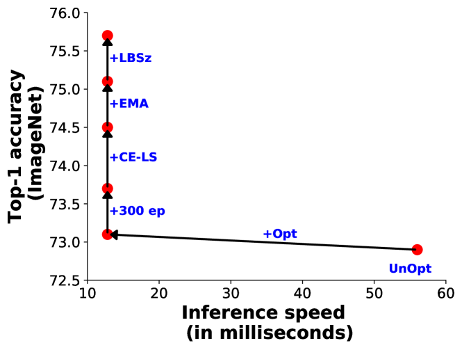
In previous experiments, we follow the experimental setup similar to ESPNetv2 and ShuffleNetv2 i.e., each model is trained for 150 epochs using a batch size of 512 and minimizes cross-entropy loss using SGD. Recent efficient models (e.g., MobileNetv3 and MNASNet) are trained longer (600 epochs) with extremely large batch size (4096) using cross-entropy with label smoothing (CE-LS) and exponential moving average (EMA). We also trained DiCENet with CE-LS and EMA, with an exception to batch size (2048) and number of epochs (300). For training with larger batch size, we accumulated the gradients for 4 iterations. This resulted in an effective batch size of 2048 (128 images per NVIDIA GTX 1080 Ti GPU $\times$ 4 GPUs $\times$ accumulation frequency of 4). Figure 8 shows the effect of these changes. Similar to state-of-the-art models (e.g., MobileNetv2, MobileNetv3, MixNet, and MNASNet), DiCENet also benefits from these hyper-parameters and yields a top-1 accuracy of 75.7 on the ImageNet.

Importantly, the optimized CUDA kernel (Figure 7) improved the inference speed drastically over the unoptimized version. This is because the optimized kernel launches one kernel for these three branches compared to one per branch in the unoptimized one and also, maximizes work done per CUDA thread. This reduces latency. With optimized CUDA kernels, DiCENet models (10-300 MFLOPs) takes between one and three days for training on the ImageNet dataset on 4 NVIDIA GTX 1080 Ti GPUs with an effective batch size of 2048.

6 Evaluating DiCENet on the ImageNet

In this section, we evaluate the performance of DiCENet on the ImageNet dataset and show that DiCENet delivers significantly better performance than state-of-the-art efficient networks, including neural search architectures. Recall that the DiCENet is ShuffleNetv2 with the DiCE unit (Section 3.4).

Implementation details: We scale the number of output channels by a width scaling factor $s$ to obtain DiCENet models at different complexity levels, ranging from 6 MFLOPs to 500+ MFLOPs (see Appendix A for details).

Evaluation metrics and baselines: We use $224\times 224$ single crop top-1 accuracy to evaluate the performance on the validation set. The performance of DiCENet is compared with state-of-the-art manually designed efficient networks (MobileNets [7, 10], ShuffleNetv2 [16], CondenseNet [41], and ESPNetv2 [11]) and automatically designed networks (MNASNet [12], FBNet [13], MixNet [15], and MobileNetv3 [14]).

Results: Recent studies (e.g., MobileNetv3) have shown that longer training with extremely large batch sizes improves performance. To have fair comparisons with state-of-the-art methods, we report the performance of DiCENet on two settings. The first setting, DiCENet-E150-B512, is similar to networks like ESPNetv2, ShuffleNetv2, and CondenseNet where DiCENet is trained for fewer epochs (150) with a smaller batch size (512) without EMA and label smoothing. The second setting, DiCENet-E300-B2048, is similar to networks like MobileNets, MNASNet, and MixNet, where DiCENet is trained for 300 epochs with a batch size of 2048. Table IV compares the performance of DiCENet with state-of-the-art efficient architectures at different FLOP ranges.

Compared to networks that are trained with smaller batch sizes and fewer epochs, e.g., ESPNetv2 (epochs: 300; batch size: 512) and ShuffleNetv2 (epochs: 240 and batch size: 1024), DiCENet delivers better performance across different FLOP ranges. Similarly, when DiCENet is trained for longer with larger batch sizes, it delivered similar or better performance than state-of-the-art methods, including neural architecture search (NAS)-based methods. For about 300 MFLOPs, DiCENet is 4% more accurate than MobileNetv2. Specifically, we observe that DiCENet is very effective when model size is small (FLOPs $<$ 150 M). For example, DiCENet outperforms MNASNet [12], FBNet [13], and MobileNetv3 [14] by 6.1%, 3.2%, and 1.1% for network size of about 70 MFLOPs, respectively.

Overall, these results shows that DiCE unit learns better representations than separable convolutions. We believe that incorporating the DiCE unit with NAS would yield better network.

Inference speed: We measure the inference time on two GPUs: (1) embedded or mobile GPU (NVIDIA GTX 960M) and (2) desktop GPU (NVIDIA GTX 1080 Ti)⁴⁴4We do not measure the inference speed on Smartphones because efficient implementations of DiCE unit are not yet available for such devices.. DiCENet is as fast as ShuffleNetv2 but delivers better performance. Compared to MobileNetv2 and MobileNetv3, DiCENet has low latency while delivering similar or better performance. We observe that MobileNetv2 and MobileNetv3 models are slow in comparison to ShuffleNetv2 and DiCENet when the batch size increases. This is because the number of channels in the depth-wise convolution in the inverted residual block of MobileNetv2 and MobileNetv3 are very large as compared to DiCENet and ShuffleNetv2. For example, the maximum number of channels in depth-wise convolution in MobileNetv2 (300 MFLOPs) are 960 while the maximum number of channels in DimConv and depth-wise convolution in DiCENet (298 MFLOPs) and ShuffleNetv2 (292 MFLOPs) are 576 and 352, respectively.

7 Task-level Generalization of DiCENet

Several previous works (e.g., [43, 44]) have shown that high accuracy on the Imagenet dataset does not necessarily correlates with high accuracy on visual scene understanding tasks (e.g., object detection and semantic segmentation). Since these tasks are widely used in real-world applications (e.g., autonomous wheel chair and robots) and often run on resource-constrained devices (e.g., embedded devices), it is important that efficient networks generalizes well on these tasks. Therefore, we evaluate the performance of DiCENet on three different tasks: (1) object detection (Section 7.1), (2) semantic segmentation (Section 7.2), and (3) multi-object classification (Section 7.3). Compared to existing efficient networks that are built using separable convolutions (e.g., MobileNets [7, 10, 14], MixNet [15], and ESPNetv2 [11]), DiCENet delivers better performance.

7.1 Object Detection on VOC and MS-COCO

Implementation details: For object detection, we use Single Shot object Detection (SSD) [17] pipeline. We use DiCENet (298 MFLOPs) pretrained on the ImageNet as a base feature extractor instead of VGG [2]. We fine-tune our network using SGD with smooth L1 and cross-entropy losses for object localization and classification, respectively.

Evaluation metrics and baselines: We evaluate the performance using mean Average Precision (mAP). For MS-COCO, we report mAP@IoU of 0.50:0.95. For SSD as a detection pipeline, we compare DiCENet’s performance with two types of base feature extractors: (1) manual (VGG [2], MobileNet [7], MobileNetv2 [10], and ESPNetv2 [11]) and (2) NAS-based (MNASNet [12], MixNet [15], and MobileNetv3 [14]).

Results: Table VI compares quantitative results of SSD with different backbone networks on the PASCAL VOC 2007 and the MS-COCO datasets. DiCENet significantly improves the performance of SSD-based object detection pipeline and delivers 1-4% higher mAP than other existing efficient variants of SSD, including NAS-based backbones such as MobileNetv3 (22.0 vs. 25.1) and MixNet (22.3 vs. 25.1). Compared to standard SSD with VGG as backbone, DiCENet achieves higher mAP while being $\mathbf{45\times}$ and $\mathbf{38\times}$ more efficient on the PASCAL VOC 2007 and the MS-COCO dataset, respectively.

SSD backbone	Image	VOC07		MS-COCO
SSD backbone	size	FLOPs	mAP	FLOPs	mAP
VGG [2]	512x512	90.2 B	74.9	99.5 B	26.8
VGG [2]	300x300	31.3 B	72.4	35.2 B	23.2
MobileNet [7]	320x320	–	–	1.3 B	22.2
MobileNetv2 [10]	320x320	–	–	0.8 B	22.1
ESPNetv2 [11]	512x512	2.5 B	75.0	3.2 B	26.0
ESPNetv2 [11]	256x256	0.9 B	70.3	1.1 B	21.9
DiCENet (Ours)	512x512	2.0 B	77.2	2.6 B	28.0
DiCENet (Ours)	300x300	0.7 B	71.9	0.9 B	25.1
MobileNetv3 [14] (NAS)	–	–	–	0.6 B	22.0
MixNet [15] (NAS)	–	–	–	0.9 B	22.3
MNASNet [12] (NAS)	–	–	–	0.8 B	23.0

TABLE VI: Object detection results of SSD [17] with different backbones on PASCAL VOC 2007 and MS-COCO. On the MS-COCO dataset, total network parameters in SSD with different backbones are about 5 million, except VGG. See Appendix B for qualitative results.

7.2 Semantic Segmentation on PASCAL VOC

Implementation details: We adapt DiCENet to ESPNetv2’s [11] encoder-decoder architecture. We choose this network because it delivers competitive performance to existing methods even with low resolution images (e.g. 256 $\times$ 256 vs. 512 $\times$ 512). We replace the encoder in ESPNetv2 (pretrained on ImageNet) with the DiCENet and follow the same training procedure for fine-tuning as ESPNetv2. We do not change the decoder.

Evaluation metrics and baselines: The performance at different complexity levels (FLOPs) is evaluated using mean intersection over union (mIOU).

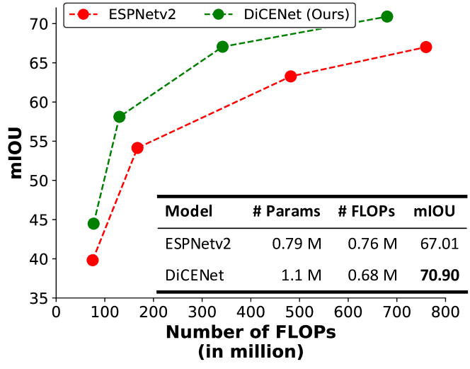
Results: Figure 9 compares the performance of DiCENet with ESPNetv2 on the PASCAL VOC 2012 validation set. DiCENet significantly improves the segmentation performance i.e., for similar FLOPs, DiCENet achieves higher mIOU while for similar mIOU, DiCENet requires significantly fewer FLOPs.

Network	# Params	# FLOPs	F1-score
Network	# Params	# FLOPs	Class-wise	Overall
ShuffleNetv2 [16]^†	3.5 M	300 M	60.42	67.58
ESPNetv2 [11]^†	3.5 M	284 M	63.41	69.23
DiCENet (ours)	5.1 M	298 M	66.92	73.41

TABLE VII: Multi-object classification results on the MS-COCO dataset. Here, ^† indicates that results are from [11].

7.3 Multi-object Classification on MS-COCO

Implementation details: Following [11], we fine-tune DiCENet using the binary cross-entropy loss.

Evaluation metrics and baselines: Similar to [11], we evaluate the performance using overall and per-class F1 score and compare with two efficient architectures, i.e., ESPNetv2 and ShuffleNetv2.

Results: Table VII shows that DiCENet outperforms existing efficient networks by a significant margin (e.g., ESPNetv2 and ShuffleNetv2 by 4.1% and 5.8% respectively) on this task.

8 Conclusion

We introduce a novel and generic convolutional unit, the DiCE unit, that uses dimension-wise convolutions and dimension-wise fusion module to learn spatial and channel-wise representations efficiently. Our empirical results suggest that the DiCE unit is more effective than separable convolutions. Moreover, when we stack DiCE units to build DiCENet model, we observe significant improvements across different computer vision tasks. We have shown that the DiCE unit is effective. Future work involves adding the DiCE unit in neural search space to discover a better neural architecture, particularly with [12, 15, 14].

Acknowledgments

This research was supported by ONR N00014-18-1-2826, DARPA N66001-19-2-403, NSF (IIS-1616112, IIS1252835), an Allen Distinguished Investigator Award, Samsung GRO and gifts from Allen Institute for AI, Google, and Amazon. Authors would also like to thank members of the PRIOR team at the Allen Institute for Artificial Intelligence (AI2), the H2Lab at the University of Washington, Seattle, and anonymous reviewers for their valuable feedback and comments.

References

[1] A. Krizhevsky, I. Sutskever, and G. E. Hinton, “Imagenet classification with deep convolutional neural networks,” in NIPS, 2012.
[2] K. Simonyan and A. Zisserman, “Very deep convolutional networks for large-scale image recognition,” in ICLR, 2014.
[3] K. He, X. Zhang, S. Ren, and J. Sun, “Deep residual learning for image recognition,” in CVPR, 2016.
[4] C. Li and C. R. Shi, “Constrained optimization based low-rank approximation of deep neural networks,” in ECCV, 2018.
[5] Y. He, J. Lin, Z. Liu, H. Wang, L.-J. Li, and S. Han, “Amc: Automl for model compression and acceleration on mobile devices,” in ECCV, 2018.
[6] J. Jin, A. Dundar, and E. Culurciello, “Flattened convolutional neural networks for feedforward acceleration,” arXiv preprint arXiv:1412.5474, 2014.
[7] A. G. Howard, M. Zhu, B. Chen, D. Kalenichenko, W. Wang, T. Weyand, M. Andreetto, and H. Adam, “Mobilenets: Efficient convolutional neural networks for mobile vision applications,” arXiv preprint arXiv:1704.04861, 2017.
[8] S. Mehta, M. Rastegari, A. Caspi, L. Shapiro, and H. Hajishirzi, “Espnet: Efficient spatial pyramid of dilated convolutions for semantic segmentation,” in ECCV, 2018.
[9] F. Chollet, “Xception: Deep learning with depthwise separable convolutions,” in CVPR, 2017.
[10] M. Sandler, A. Howard, M. Zhu, A. Zhmoginov, and L.-C. Chen, “Mobilenetv2: Inverted residuals and linear bottlenecks,” in CVPR, 2018.
[11] S. Mehta, M. Rastegari, L. Shapiro, and H. Hajishirzi, “Espnetv2: A light-weight, power efficient, and general purpose convolutional neural network,” in CVPR, 2019.
[12] M. Tan, B. Chen, R. Pang, V. Vasudevan, and Q. V. Le, “Mnasnet: Platform-aware neural architecture search for mobile,” arXiv preprint arXiv:1807.11626, 2018.
[13] B. Wu, X. Dai, P. Zhang, Y. Wang, F. Sun, Y. Wu, Y. Tian, P. Vajda, Y. Jia, and K. Keutzer, “Fbnet: Hardware-aware efficient convnet design via differentiable neural architecture search,” arXiv preprint arXiv:1812.03443, 2018.
[14] A. Howard, M. Sandler, G. Chu, L.-C. Chen, B. Chen, M. Tan, W. Wang, Y. Zhu, R. Pang, V. Vasudevan, Q. V. Le, and H. Adam, “Searching for mobilenetv3,” in ICCV, October 2019.
[15] M. Tan and Q. V. Le, “Mixconv: Mixed depthwise convolutional kernels,” in BMVC, 2019.
[16] N. Ma, X. Zhang, H.-T. Zheng, and J. Sun, “Shufflenet v2: Practical guidelines for efficient cnn architecture design,” in ECCV, 2018.
[17] W. Liu, D. Anguelov, D. Erhan, C. Szegedy, S. Reed, C.-Y. Fu, and A. C. Berg, “SSD: Single shot multibox detector,” in ECCV. Springer, 2016, pp. 21–37.
[18] X. Zhang, X. Zhou, M. Lin, and J. Sun, “Shufflenet: An extremely efficient convolutional neural network for mobile devices,” in CVPR, 2018.
[19] B. Zoph and Q. V. Le, “Neural architecture search with reinforcement learning,” in ICLR, 2017.
[20] B. Zoph, V. Vasudevan, J. Shlens, and Q. V. Le, “Learning transferable architectures for scalable image recognition,” in CVPR, 2018, pp. 8697–8710.
[21] M. Wortsman, A. Farhadi, and M. Rastegari, “Discovering neural wirings,” in NeurIPS, 2019.
[22] M. Rastegari, V. Ordonez, J. Redmon, and A. Farhadi, “Xnor-net: Imagenet classification using binary convolutional neural networks,” in ECCV, 2016.
[23] J. Wu, C. Leng, Y. Wang, Q. Hu, and J. Cheng, “Quantized convolutional neural networks for mobile devices,” in CVPR, 2016.
[24] I. Hubara, M. Courbariaux, D. Soudry, R. El-Yaniv, and Y. Bengio, “Binarized neural networks,” in NIPS, 2016.
[25] R. Andri, L. Cavigelli, D. Rossi, and L. Benini, “Yodann: An architecture for ultralow power binary-weight cnn acceleration,” IEEE Transactions on Computer-Aided Design of Integrated Circuits and Systems, 2018.
[26] S. Han, H. Mao, and W. J. Dally, “Deep compression: Compressing deep neural networks with pruning, trained quantization and huffman coding,” in ICLR, 2016.
[27] W. Wen, C. Wu, Y. Wang, Y. Chen, and H. Li, “Learning structured sparsity in deep neural networks,” in NIPS, 2016.
[28] A. Veit and S. Belongie, “Convolutional networks with adaptive inference graphs,” in ECCV, 2018.
[29] G. Hinton, O. Vinyals, and J. Dean, “Distilling the knowledge in a neural network,” in NIPS Deep Learning and Representation Learning Workshop, 2015.
[30] S. Gupta, J. Hoffman, and J. Malik, “Cross modal distillation for supervision transfer,” in CVPR, 2016, pp. 2827–2836.
[31] J. Yim, D. Joo, J. Bae, and J. Kim, “A gift from knowledge distillation: Fast optimization, network minimization and transfer learning,” in CVPR, 2017, pp. 4133–4141.
[32] B. Jacob, S. Kligys, B. Chen, M. Zhu, M. Tang, A. Howard, H. Adam, and D. Kalenichenko, “Quantization and training of neural networks for efficient integer-arithmetic-only inference,” in CVPR, 2018, pp. 2704–2713.
[33] K. Wang, Z. Liu, Y. Lin, J. Lin, and S. Han, “Haq: Hardware-aware automated quantization with mixed precision,” in CVPR, 2019, pp. 8612–8620.
[34] J. Hu, L. Shen, and G. Sun, “Squeeze-and-excitation networks,” in CVPR, 2018, pp. 7132–7141.
[35] O. Russakovsky, J. Deng, H. Su, J. Krause, S. Satheesh, S. Ma, Z. Huang, A. Karpathy, A. Khosla, M. Bernstein, A. C. Berg, and L. Fei-Fei, “ImageNet Large Scale Visual Recognition Challenge,” IJCV, 2015.
[36] T.-Y. Lin, M. Maire, S. Belongie, J. Hays, P. Perona, D. Ramanan, P. Dollár, and C. L. Zitnick, “Microsoft coco: Common objects in context,” in ECCV, 2014.
[37] M. Everingham, L. Van Gool, C. K. I. Williams, J. Winn, and A. Zisserman, “The PASCAL Visual Object Classes Challenge 2007 (VOC2007) Results,” 2007.
[38] M. Everingham, S. A. Eslami, L. Van Gool, C. K. Williams, J. Winn, and A. Zisserman, “The pascal visual object classes challenge: A retrospective,” IJCV, 2015.
[39] B. Hariharan, P. Arbeláez, L. Bourdev, S. Maji, and J. Malik, “Semantic contours from inverse detectors,” in ICCV, 2011.
[40] S. Xie, R. Girshick, P. Dollár, Z. Tu, and K. He, “Aggregated residual transformations for deep neural networks,” in CVPR, 2017.
[41] G. Huang, S. Liu, L. van der Maaten, and K. Q. Weinberger, “Condensenet: An efficient densenet using learned group convolutions,” in CVPR, 2018.
[42] R. Wightman, “PyTorch Image Models.” [Online]. Available: https://github.com/rwightman/pytorch-image-models
[43] J. Long, E. Shelhamer, and T. Darrell, “Fully convolutional networks for semantic segmentation,” in CVPR, 2015.
[44] Z.-Q. Zhao, P. Zheng, S.-t. Xu, and X. Wu, “Object detection with deep learning: A review,” IEEE transactions on neural networks and learning systems, 2019.
[45] S. Ioffe and C. Szegedy, “Batch normalization: Accelerating deep network training by reducing internal covariate shift,” arXiv preprint arXiv:1502.03167, 2015.
[46] K. He, X. Zhang, S. Ren, and J. Sun, “Delving deep into rectifiers: Surpassing human-level performance on imagenet classification,” in ICCV, 2015.
[47] S. Mehta, R. Koncel-Kedziorski, M. Rastegari, and H. Hajishirzi, “Pyramidal recurrent unit for language modeling,” in Proceedings of the 2018 Conference on Empirical Methods in Natural Language Processing. Association for Computational Linguistics, 2018.

Appendix A Network Architecture

The overall architecture at different network complexities is given in Table VIII. The first layer is a standard $3\times 3$ convolution with a stride of two while the second layer is a max pooling layer. All convolutional layers are followed by a batch normalization layer [45] and a PReLU non-linear activation layer [46], except for the last layer that feeds into a softmax for classification. Following previous work [7, 10, 16, 18, 11], we scale the number of output channels by a width scaling factor $s$ to construct networks at different FLOPs. We initialize weights of our network using the same method as in [46].

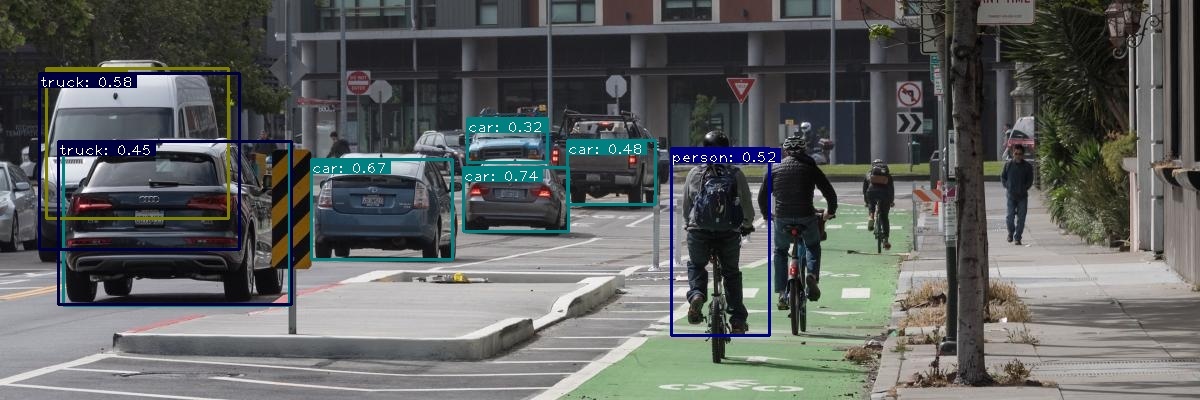
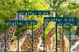
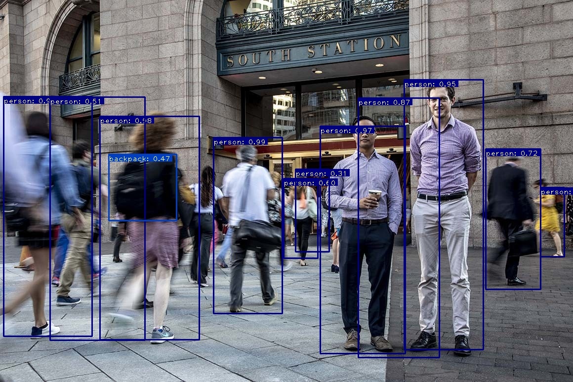
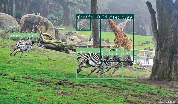
Appendix B Qualitative Results for Object Detection and Semantic Segmentation

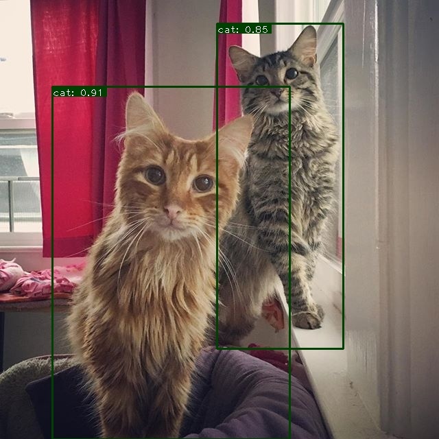
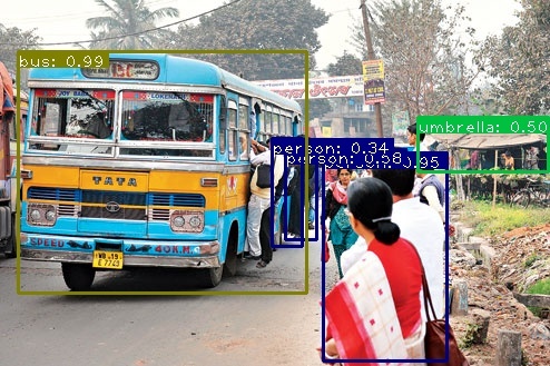
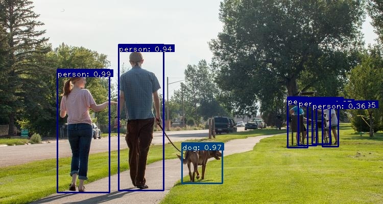
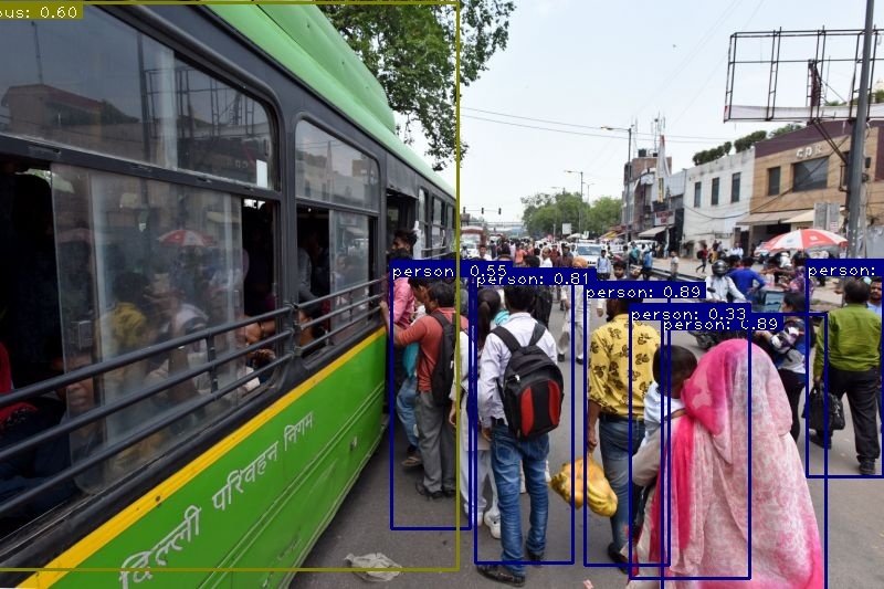
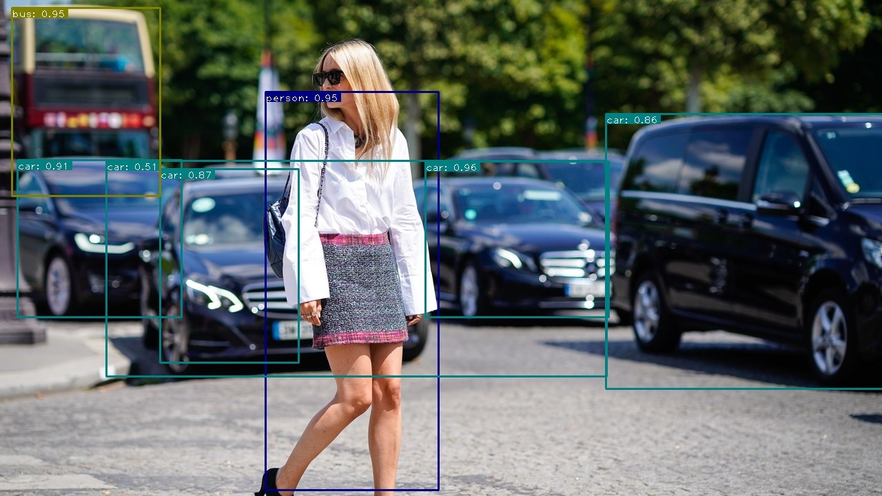
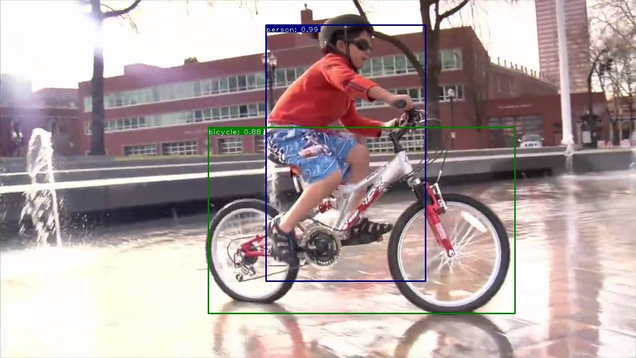
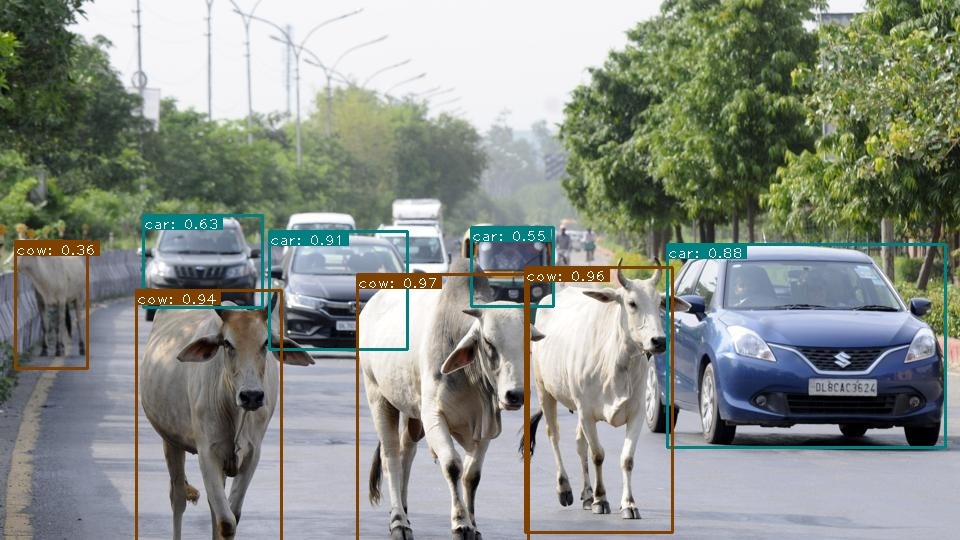
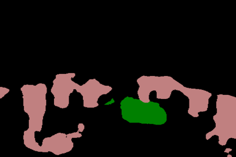
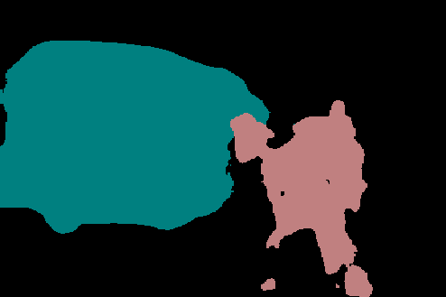
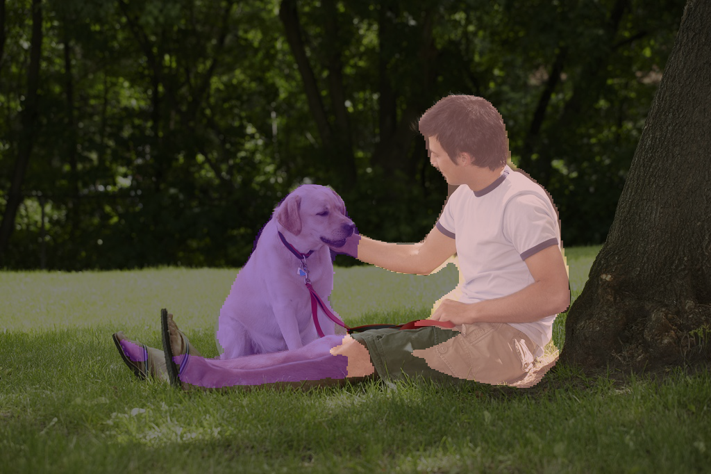
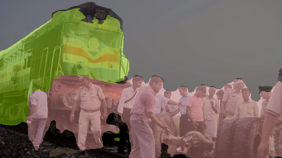
Figure 10 provides qualitative results for object detection while Figures 11 provide results for semantic segmentation on the PASCAL VOC 2012 dataset as well as in the wild. These results suggest that the DiCENet is able to detect and segment objects in diverse settings, including different backgrounds and image sizes.

Layer	Output size	Kernel size	Stride	Repeat	Output channels (network width scaling parameter $s$ )
Layer	Output size	Kernel size	Stride	Repeat	$s=0.1$	$s=0.2$	$s\in\left[0.5,2.0\right]$	$s=2.4$
Image	$224\times 224$				3	3	3	3
Conv1	$112\times 112$	$3\times 3$	2	1	8	16	24	24
Max Pool	$56\times 56$	$3\times 3$	2		8	16	24	24
Block 1	$28\times 28$		2	1	16	32	116 $\times s$	278
Block 1	$28\times 28$		1	3	16	32	116 $\times s$	278
Block 2	$14\times 14$		2	1	32	64	232 $\times s$	556
Block 2	$14\times 14$		1	7	32	64	232 $\times s$	556
Block 3	$7\times 7$		2	1	64	128	464 $\times s$	1112
Block 3	$7\times 7$		1	3	64	128	464 $\times s$	1112
Global Pool	$1\times 1$	$7\times 7$			512	1024	1024	1280
Grouped FC [47]	$1\times 1$	$1\times 1$	1	1	512	1024	1024	1280
FC					1000	1000	1000	1000
FLOPs					6.5 M	12 M	24-240 M	298 M

TABLE VIII: Overall architecture of DiCENet (ShuffleNetv2 with DiCE unit) at different network complexities for the ImageNet classification. We use 4 groups in grouped fully connected (FC) layer. For other architecture designs in Figure 5 on the paper (MobileNetv1 and ResNet), we replace blocks 1, 2, and 3 with the corresponding blocks.