Revealing the system-bath coupling via Landau-Zener-Stückelberg interferometry in superconducting qubits

Abstract

In this work we propose a way to unveil the type of environmental noise in strongly driven superconducting flux qubits through the analysis of the Landau-Zener-Stückelberg (LZS) interferometry. We study both the two-level and the multilevel dynamics of the flux qubit driven by a dc+ac magnetic field. We found that the LZS interference patterns exhibit well defined multiphoton resonances whose shape strongly depend on the time scale and the type of coupling to a quantum bath. For the case of transverse system-bath coupling, the n-photon resonances are narrow and nearly symmetric with respect to the dc magnetic field for almost all time scales, whilst in the case of longitudinal coupling they exhibit a change from a wide symmetric to an antisymmetric shape for times of the order of the relaxation time. We find this dynamic behavior relevant for the interpretation of several LZS interferometry experiments in which the stationary regime is not completely reached.

Superconducting circuits with Josephson junctions Orlando et al. (1999); Chiorescu et al. (2003) behave as artificial atoms You and Nori (2011) and have been extensively proven as quantum bits Makhlin et al. (2001). When driven by a dc+ac magnetic flux, Landau-Zener-Stückelberg (LZS) interference patterns Shevchenko et al. (2010) combined with multi-photon resonances have been observed Oliver et al. (2005); Berns et al. (2006, 2008); Oliver and Valenzuela (2009); Izmalkov et al. (2008) and used to probe the energy level spectrum of the device for large driving amplitudes. Berns et al. (2008); Oliver and Valenzuela (2009). LZS patterns also emerge in charge qubitsSillanpää et al. (2006); Wilson et al. (2007), Rydberg atomsYoakum et al. (1992), ultracold molecular gasesMark et al. (2007), optical latticesKling et al. (2010) and single electron spins systemsHuang et al. (2011). In addition, LZS interferometry was recently proposed as a tool to determine relevant information related to the coupling of a qubit with a noisy environment, such as dissipation strength and dephasing time Forster et al. (2014); Blattmann et al. (2015); Mi et al. (2018). These studies have been performed for steady state-experiments, where full relaxation with the bath degrees of freedom is assumed.

In the present work we demonstrate that the finite time LZS spectroscopy can unveil additional features linked to how relevant times scales affect the symmetry of the resonance patterns for different system-bath couplings. As a system of study we chose the superconducting Flux Qubit (FQ) originally introduced in Ref.[Orlando et al., 1999] and which over the last years, due to the improvement in its design and fabrication techniques, has become one of the most tested devices for quantum information proposals Yan et al. (2016). Recent experiments on the FQ have implemented noise spectroscopy for different sources of noise (flux noise, charge noise, critical current noise) through dynamical decoupling Bylander et al. (2011) and driven evolution measurements Yan et al. (2013); Yoshihara et al. (2014).

Here to address the finite time LZS interferometry we study the FQ coupled to a quantum bath and under strong periodic driving, using the Floquet-Markov quantum master equations Grifoni and Hänggi (1998); Kohler et al. (1998). Our main finding is that a dynamic change in the symmetry of a n-photon resonance takes place for the case of longitudinal system-bath coupling, whilst the resonances remain almost undisturbed in time for transverse system-bath coupling.

Our analysis becomes particularly relevant to understand LZS interferometry experiments for FQ with large relaxation times Oliver et al. (2005); Oliver and Valenzuela (2009). Several well established theoretical works have studied the steady state of periodically driven two level systems Hartmann et al. (2000); Dakhnovskii et al. (1995); Stace et al. (2005); Goorden et al. (2004); Hausinger and Grifoni (2010). However, the experimental results on LZS interferometry in the FQ do not agree with these previous theoretical results. The theory of Hartmann et al. (2000); Dakhnovskii et al. (1995); Stace et al. (2005); Goorden et al. (2004); Hausinger and Grifoni (2010) shows population inversion and antisymmetric resonance patterns as a function of the energy detuning, instead of the symmetric patterns observed in the FQ experiments Oliver et al. (2005); Oliver and Valenzuela (2009). A possible explanation was put forward in Refs.Ferrón et al. (2012, 2016): there is a dynamic transition from symmetric resonance patterns below the relaxation time $t_{r}$ to antisymmetric resonance patterns for time scales above $t_{r}$. Since the FQ experiments were performed at finite times scales below $t_{r}$, the steady state patterns were not observed, according to this scenario. On the other hand, in Ref.[Blattmann et al., 2015] it was shown that transverse noise (previous works Hartmann et al. (2000); Dakhnovskii et al. (1995); Stace et al. (2005); Goorden et al. (2004); Hausinger and Grifoni (2010); Ferrón et al. (2012, 2016) considered longitudinal noise) can lead to steady state symmetric resonances in LZS interferometry, which suggest a different possible explanation of the experimental results. The aim of this work is to assess which scenario is more adequate to explain the experiments of Refs.Oliver et al. (2005); Oliver and Valenzuela (2009) by analyzing the time dependence of the LZS patterns for different system-bath couplings (transverse and longitudinal noise).

We start in Sec. I by writing the Hamiltonian of the FQ in the presence of different sources of quantum noise and describing the Floquet-Markov formulation for open quantum systems with a time periodic drive. In Sec. II we show results for the time dependent evolution of the driven FQ with different sources of noise, restricted to a two levels system (TLS) regime. In Sec. III we extend the analysis to the multilevel case, which is relevant for large driving amplitudes and to compare with LZS experiments. Conclusions are given in Sec. IV.

I Dynamics of the Flux Qubit

I.1 The Flux Qubit and noise sources

The FQ consists on a superconducting ring with three Josephson junctionsOrlando et al. (1999) enclosing a magnetic flux $\Phi=f\Phi_{0}$ ($\Phi_{0}=h/2e$) with phase differences $\varphi_{1}$, $\varphi_{2}$ and $\varphi_{3}=-\varphi_{1}+\varphi_{2}-2\pi f$. Two of the junctions have coupling energy, $E_{J}$, and capacitance, $C$, while the third has $E_{J,3}=\alpha E_{J}$ and $C_{3}=\alpha C$. In the quantum regime, the FQ Hamiltonian reads:Orlando et al. (1999)

$${{\cal H}}_{FQ}=E_{p}{n}_{p}^{2}+E_{m}{n}_{m}^{2}+E_{J}{V}\;,$$ (1)

with $\varphi_{p}=\frac{\varphi_{1}+\varphi_{2}}{2}$ and $\varphi_{m}=\frac{\varphi_{1}-\varphi_{2}}{2}$ the phase operators, ${n}_{k}=-i\frac{\partial}{\partial\varphi_{k}}$ ($k=p,m$) the charge number operators, $E_{p}=2E_{C}$, $E_{m}=\frac{E_{p}}{1+2\alpha}$, $E_{C}=e^{2}/2C$ and ${V}(\varphi_{p},\varphi_{m};f)=2+\alpha-2\cos\varphi_{p}\cos\varphi_{m}-\alpha\cos(2\pi f+2\varphi_{m})$. The FQ has several levels with eigenenergies $E_{i}$ and eigenstates $|\Psi_{i}\rangle$ which depend on $\alpha$, $\eta=\sqrt{8E_{C}/E_{J}}$ and flux detuning ${\tilde{f}}=f-1/2$. Typical experiments have $\alpha\sim 0.6-0.9$ and $\eta\sim 0.1-0.6$ Chiorescu et al. (2003); Oliver et al. (2005); Berns et al. (2006, 2008); Oliver and Valenzuela (2009). For $\alpha\geq 1/2$ and $|{\tilde{f}}|\ll 1$, the potential ${V}$ has the shape of a double-well with two minima along the $\varphi_{l}$ direction. Each minima corresponds to macroscopic persistent currents of opposite sign, and for ${\tilde{f}}\gtrsim 0$ (${\tilde{f}}\lesssim 0$) a ground state with positive (negative) loop current is favored. In this regime the system can be operated as a quantum bitOrlando et al. (1999); Chiorescu et al. (2003) and approximated by a two-level system (TLS)Orlando et al. (1999); Ferrón and Domínguez (2010).

The main sources of relaxation and decoherence in the FQ are flux noise $\delta f(t)$, charge noise $\delta N(t)$, and critical current noise $\delta{I}_{c}(t)$ You et al. (2007); Yan et al. (2013); Yoshihara et al. (2014); Bylander et al. (2011); Sete et al. (2017). In the case of weak fluctuations, the different sources of noise can be incorporated in Eq.(1) by the replacements $f\rightarrow f+{\delta f}$, ${n}_{k}\rightarrow{n}_{k}-{\delta N}_{k}$ ($k=p,m$), and $E_{J}\rightarrow E_{J}(1+{\delta I_{c}}/{I}_{c})$, respectively You et al. (2007); Yan et al. (2013); Yoshihara et al. (2014); Bylander et al. (2011). This leads to ${\cal H}_{FQ}\rightarrow{\cal H}_{FQ}^{\prime}\approx{\cal H}_{FQ}+{H}_{int}$, where

$${H}_{int}={H}_{int}^{ch}+{H}_{int}^{f}+{H}_{int}^{cc}\;,$$ (2)

and

$${H}_{int}^{ch} = -2E_{p}{n}_{p}\delta{N}_{p}-2E_{m}{n}_{m}\delta{N}_{m}\;,$$

$${H}_{int}^{f} = -{2\pi E_{J}}{I}\delta{f}\;,$$

$${H}_{int}^{cc} = \frac{E_{J}}{I_{c}}{V}\delta{I_{c}}\;,$$ (3)

with ${I}=\alpha\sin(2\pi{\tilde{f}}+2{\varphi}_{m})$, the loop current operator normalized by $I_{c}=\frac{2\pi E_{J}}{\Phi_{0}}$. Notice that Eq.(2) results from neglecting quadratic terms in $({n}_{p}-{N}_{p})^{2}$ and $({n}_{m}-{N}_{m})^{2}$, since we are assuming the weak fluctuations regime.

If we consider the lowest eigenstates, the term with ${n}_{p}$ can be neglectedfoo and we can redefine the system-bath interaction Hamiltonian as

$${H}_{int}={\cal A}^{ch}\otimes{\cal B}^{ch}+{\cal A}^{f}\otimes{\cal B}^{f}+{\cal A}^{cc}\otimes{\cal B}^{cc},$$ (4)

where the system operators are ${\cal A}^{ch}=-2E_{m}{n}_{m}$, ${\cal A}^{f}=-{2\pi E_{J}}{I}$, ${\cal A}^{cc}=E_{J}{V}$; and the normalized bath (noise) operators are ${\cal B}^{ch}=\delta{N}_{p}$, ${\cal B}^{f}=\delta{f}$ and ${\cal B}^{cc}=\delta{I_{c}}/I_{c}$.

As a first approach we will consider in Sec. II the FQ restricted to the two-lowest computational levels, Orlando et al. (1999); Ferrón and Domínguez (2010)

$${\cal H}_{TLS}=-\frac{\epsilon}{2}{\sigma}_{z}-\frac{\Delta}{2}{\sigma}_{x}\;,$$ (5)

where the Hamiltonian is written in the basis defined by the persistent current states $|+\rangle=(|0\rangle+|1\rangle)/\sqrt{2}$ and $|-\rangle=(|0\rangle-|1\rangle)/\sqrt{2}$, where $|0\rangle$ and $|1\rangle$ are the ground and excited FQ states at $\delta f=0$. The parameters of ${\cal H}_{TLS}$ are the detuning $\epsilon=4\pi I_{p}{\tilde{f}}$, and the energy gap $\Delta=E_{1}-E_{0}$ at ${\tilde{f}}=0$. Here $I_{p}=|\langle+|{I}|+\rangle|=|\langle-|{I}|-\rangle|$ is the magnitude of the loop current. Within this approximation, the noise coupling operators become

$${\mathcal{A}}^{f} = -\lambda_{f}{\sigma}_{z},$$

$${\mathcal{A}}^{ch} = -\lambda_{ch}{\sigma}_{y},$$

$${\mathcal{A}}^{cc} = -\lambda_{cc}{\sigma}_{x},\,,$$ (6)

with $\lambda_{f}=2\pi|\langle+|{I}|+\rangle|$, $\lambda_{ch}=\frac{\eta^{2}}{4+8\alpha}|\langle-|{n}_{m}|+\rangle|$ and $\lambda_{cc}=-|\langle-|{V}|+\rangle|$.

For the parameter values $\alpha=0.8$ and $\eta=0.25$ and after diagonalization of ${\cal H}_{TLS}$, we obtain $I_{p}=0.721$ (in units of $E_{J}/\Phi_{0}$) and $\Delta=3.33\times 10^{-4}$ (in units of $E_{J}$). Thus, the noise coupling parameters results $\lambda_{f}\approx 4.5$, $\lambda_{ch}\approx 3\times 10^{-4}$, and $\lambda_{cc}\approx 4\times 10^{-3}$ (the neglected term corresponding to ${n}_{p}$ has coupling parameter $\lambda^{p}_{ch}=\frac{\eta^{2}}{4}|\langle-|{n}_{p}|+\rangle|\approx 10^{-13}$).

I.2 LZS interferometry in the presence of quantum noise: The Floquet-Markov approach

In experiments with flux qubits, LZS interferometry Oliver et al. (2005); Berns et al. (2006, 2008); Oliver and Valenzuela (2009); Rudner et al. (2008) is performed applying an harmonic (ac) field of frequency $\omega_{0}$ on top of the static flux, i.e.

$${\tilde{f}}\rightarrow{\tilde{f}}(t)={\tilde{f}}_{dc}+f_{ac}\cos{(\omega_{0}t)}\;.$$ (7)

In this work, and following Refs.[Shirley, 1965; Grifoni and Hänggi, 1998; Breuer et al., 2000; Hone et al., 2009; Hausinger and Grifoni, 2010; Ferrón et al., 2010, 2012, 2016] we analyze the LZS interferometry employing the Floquet formalism, which allows for an exact treatment of harmonic drivings of arbitrary strength and frequency. Alternative approaches to the description of the LZS interference patterns rely on approximations valid either for large driving frequencies or low driving amplitudes Berns et al. (2006); Ashhab et al. (2007); Shevchenko et al. (2010).

For the harmonic driving, the Hamiltonian of the FQ results time periodic ${\cal H}_{FQ}(t)={\cal H}_{FQ}(t+\tau)$, with $\tau=2\pi/\omega_{0}$. In the Floquet formalism, the solutions of the Schrödinger equation are of the form $|\Psi_{\alpha}(t)\rangle=e^{i\varepsilon_{\alpha}t/\hbar}|\alpha(t)\rangle$, where the Floquet states $|\alpha(t)\rangle$ satisfy $|\alpha(t)\rangle$=$|\alpha(t+\tau)\rangle=\sum_{k}|\alpha_{k}\rangle e^{-ik\omega t}$, and are eigenstates of the equation $[{\cal H}(t)-i\hbar\partial/\partial t]|\alpha(t)\rangle=\varepsilon_{\alpha}|\alpha(t)\rangle$, with $\varepsilon_{\alpha}$ the associated quasi-energy.

Since the FQ is in contact with the environment, the total Hamiltonian of the open system is

$$H=H_{s}(t)+H_{B}+{H}_{int}.$$

Here, $H_{s}$ is the system Hamiltonian, in our case $H_{s}={\cal H}_{FQ}$, $H_{B}$ is the Hamiltonian of the environment, which is usually modeled as a bath of harmonic oscillatorsKohler et al. (1998); Breuer et al. (2000); Hone et al. (2009); Hausinger and Grifoni (2010); Goorden et al. (2004); Goorden, M. C. et al. (2005); van der Wal, C. H. et al. (2003), and ${H}_{int}$ is the system-bath interaction Hamiltonian. For weak coupling (Born approximation) and fast bath relaxation (Markov approximation), a Floquet-Born-Markov master equation for the system reduced density matrix $\rho$ in the Floquet basis, $\rho_{\alpha\beta}(t)=\langle\alpha(t)|\rho(t)|\beta(t)\rangle$, can be obtainedKohler et al. (1998); Breuer et al. (2000); Hone et al. (2009):

$$\frac{d\rho_{\alpha\beta}(t)}{dt} = \sum_{\alpha^{\prime}\beta^{\prime}}\Lambda_{\alpha\beta\alpha^{\prime}\beta^{\prime}}\;\rho_{\alpha^{\prime}\beta^{\prime}}\,,$$

$$\Lambda_{\alpha\beta\alpha^{\prime}\beta^{\prime}} = -\frac{i}{\hbar}(\varepsilon_{\alpha}-\varepsilon_{\beta})\delta_{\alpha\alpha^{\prime}}\delta_{\beta\beta^{\prime}}+L_{\alpha\beta\alpha^{\prime}\beta^{\prime}}\;.$$ (8)

The coefficients ${\it L}_{\alpha\beta\alpha^{\prime}\beta^{\prime}}$ are usually rewritten in terms of transition rates $R_{\alpha\beta\alpha^{\prime}\beta^{\prime}}$ as

$${\it L}_{\alpha\beta\alpha^{\prime}\beta^{\prime}} = R_{\alpha\beta\alpha^{\prime}\beta^{\prime}}+R_{\beta\alpha\beta^{\prime}\alpha^{\prime}}^{*}$$

$$-\sum_{\eta}\left(\delta_{\beta\beta^{\prime}}R_{\eta\eta\alpha^{\prime}\alpha}+\delta_{\alpha\alpha^{\prime}}R_{\eta\eta\beta^{\prime}\beta}^{*}\right).$$

As we already shown in Eq.(4), the interaction Hamiltonian can be written as

$${H}_{int}=\sum_{\nu}{\cal A}^{\nu}\otimes{\cal B}^{\nu},$$

where the ${\cal A}^{\nu}$ are system operators and the ${\cal B}^{\nu}$ are bath operators associated to different noise sources. In the case of independent noise sources, the corresponding bath operators are uncorrelated such that $\langle{\cal B^{\nu}}(t){\cal B}^{\nu^{\prime}}(t^{\prime})\rangle=0$ for $\nu\not=\nu^{\prime}$, and the transition rates $R_{\alpha\beta\alpha^{\prime}\beta^{\prime}}$ are given as

$$R_{\alpha\beta\alpha^{\prime}\beta^{\prime}}=\sum_{\nu}R_{\alpha\beta\alpha^{\prime}\beta^{\prime}}^{\nu},$$

with

$$R_{\alpha\beta\alpha^{\prime}\beta^{\prime}}^{\nu}=\sum_{q}g^{\nu}(\omega_{\alpha\alpha^{\prime},q})A_{\alpha\alpha^{\prime},q}^{\nu}A_{\beta^{\prime}\beta,-q}^{\nu}\,,$$ (10)

where $\omega_{\alpha\alpha^{\prime},q}=(\varepsilon_{\alpha}-\varepsilon_{\alpha}^{\prime})/\hbar+q\omega_{0}$. In this way, the system-bath interaction is encoded in the transition matrix elements

$$A_{\alpha\beta,q}^{\nu}=\sum_{k}\langle\alpha_{k}|{\cal A}^{\nu}|\beta_{k+q}\rangle.$$

Assuming that each bath is in equilibrium at temperature $T^{\nu}$ it is customary to define:

$$g^{\nu}({\omega})=\int_{-\infty}^{\infty}dt\langle{\cal B^{\nu}}(t){\cal B^{\nu}}(0)\rangle e^{-i\omega t}=J^{\nu}(\omega)n_{\rm th}^{\nu}(\hbar\omega),$$

where $J^{\nu}(\omega)$ [defining $J^{\nu}(-\omega)=-J^{\nu}(\omega)$] is the bath spectral density and $n_{\rm th}^{\nu}(\varepsilon)=1/[\exp{(\varepsilon/k_{B}T^{\nu})}-1]$ com .

In this work, we compute numerically the Floquet states $|\alpha(t)\rangle$, and calculate the coefficients ${\it L}_{\alpha\beta\alpha^{\prime}\beta^{\prime}}$ , from which the solution of $\rho_{\alpha\beta}(t)$ can be obtained Ferrón et al. (2010, 2016).

II Two levels regime

II.1 Unitary evolution and LZS interferometry

We start by reviewing the LZS interferometry for the TLS. In order to obtain the driven Hamiltonian, we replace in ${\cal H}_{TLS}$

$$\epsilon\rightarrow\epsilon(t)=\epsilon_{0}+A\cos(\omega_{0}t),$$ (11)

with $\epsilon_{0}=4\pi I_{p}{\tilde{f}}_{dc}$ and $A=4\pi I_{p}f_{ac}$. The frequency $\omega_{0}$ is written in units of $E_{J}/\hbar$ and the qubit eigenenergies in units of $E_{J}$. When $f_{ac}>|{\tilde{f}}_{dc}|$ the central avoided crossing at ${\tilde{f}}=0$ is reached for driving amplitudes, ${\tilde{f}}_{dc}\pm f_{ac}$. In this case the periodically repeated transitions at ${\tilde{f}}=0$ give rise to the LZS interference patterns as a function of ${\tilde{f}}_{dc}$ and $f_{ac}$, characterized by multiphoton resonances at $E_{1}({\tilde{f}})-E_{0}({\tilde{f}})=n\omega_{0}$ Shevchenko et al. (2010); Grifoni and Hänggi (1998); Breuer et al. (2000); Hone et al. (2009); Hausinger and Grifoni (2010); Ashhab et al. (2007) .

For $\epsilon_{0}\gg\Delta$ the resonances take place at $\epsilon_{0}\simeq n\omega_{0}$, and denoting $f_{\omega}=\omega_{0}/4\pi I_{p}$, the $n$-resonance condition can be written as $\epsilon_{0}/\omega_{0}={\tilde{f}}_{dc}/f_{\omega}=n$.

In the regime $A\omega_{0}\gg\Delta^{2}$ and in the Rotating Wave Approximation (RWA) Shevchenko et al. (2010); Ashhab et al. (2007); Berns et al. (2006), the time averaged probability of measuring a positive loop current $\overline{P_{+}}=\overline{|\langle\Psi(t)|+\rangle|^{2}}$, near a $n-$ photon resonance results

$$\overline{P_{+}}=1-\frac{1}{2}\frac{\Delta_{n}^{2}}{(n\omega_{0}-{\epsilon}_{0})^{2}+\Delta_{n}^{2}}\;.$$ (12)

When the resonance condition $\epsilon_{0}=n\omega_{0}$ is satisfied, Eq.(12) gives $\overline{P_{+}}=1/2$, otherwise is $\overline{P_{+}}\lesssim 1$. Furthermore, the width of the resonance is $\delta\epsilon=|\Delta_{n}|=\Delta|J_{n}(A/\omega_{0})|=\Delta|J_{n}(f_{ac}/f_{\omega})|$, with $J_{n}(x)$ the Bessel function of first kind. This gives a quasi periodic dependence as a function of $f_{ac}$ for ${\tilde{f}}_{dc}$ fixed near the resonance. In particular, at the zeros of $J_{n}(x)$ the resonance is destroyed, with $\overline{P_{+}}\sim 1$ instead of $\overline{P_{+}}=1/2$, a phenomenon known as coherent destruction of tunneling Grossmann et al. (1991); Kayanuma and Saito (2008). Plots of $\overline{P_{+}}$ as a function of flux detuning ${\tilde{f}}_{dc}$ and ac amplitude $f_{ac}$ give the typical LZS interference patterns, which have been measured experimentally in flux qubits Oliver et al. (2005); Berns et al. (2006, 2008); Oliver and Valenzuela (2009); Rudner et al. (2008) and have also been observed in other driven systems Izmalkov et al. (2008); Sillanpää et al. (2006); Wilson et al. (2007, 2010); Sun et al. (2009, 2011); Wang et al. (2010); de Graaf et al. (2013); Shevchenko et al. (2012); Mark et al. (2007); Petta et al. (2010); Stehlik et al. (2012); Cao et al. (2013); Dupont-Ferrier et al. (2013); Shang et al. (2013); Nalbach et al. (2013); Forster et al. (2014); Granger et al. (2015); Huang et al. (2011); Zhou et al. (2014); LaHaye et al. (2009); Kling et al. (2010).

Several phenomenological approaches Shevchenko et al. (2010); Berns et al. (2008); Du et al. (2010); You and Nori (2011) have taken into account relaxation and decoherence effects in LZS interferometry, obtaining a broadening of the Lorentzian-shape $n-$ photon resonances of Eq.(12).

II.2 Longitudinal vs. transverse noise

In this section we analyze the environmental noise employing the Floquet Markov master equation, described in Sec.I.2. We first consider the two extreme cases: either pure flux or “longitudinal” noise (which commutes with the driving), or pure charge noise, which we call “transverse” noise. For simplicity, we consider in both cases that the baths are equilibrated at the same temperature $T^{\nu}=T$ with an ohmic spectral density $J^{\nu}(\omega)=\gamma\omega e^{-\omega/\omega_{c}}$. In the case of pure longitudinal noise we consider, ${\mathcal{A}}^{f}\rightarrow{\mathcal{A}}=-\lambda_{f}{\sigma}_{z}$ while in the case of pure transverse noise we take ${\mathcal{A}}^{ch}\rightarrow{\mathcal{A}}=-\lambda_{ch}{\sigma}_{y}$. In order to establish a quantitative comparison among the two types of noise we first analize the results for equal coupling strengths $\lambda^{(f)}=\lambda^{(ch)}=1$.

We use typical reported experimental values for FQ Oliver et al. (2005), $E_{J}/h\sim 300{\rm GHz}$, driving microwave frequency $\omega_{0}/2\pi=0.003E_{J}/\hbar\sim 900\rm{MHz}$, bath temperature $T=0.0014E_{J}/k_{B}(\sim 20{\rm mK})$ and we consider $\gamma=0.001$. Furthermore, in all the cases we are assuming that the FQ is initially prepared in its ground state $|\Psi_{0}\rangle$ of the static Hamiltonian $H_{0}\equiv{\cal H}_{FQ}({\tilde{f}}={\tilde{f}}_{dc})$. Experimentally, the probability of having a state of positive or negative persistent current in the FQ is measuredChiorescu et al. (2003); Oliver et al. (2005). The probability of a positive current measurement can be calculated as $P_{+}(t)={\rm Tr}(\Pi_{+}\rho(t))$, with $\Pi_{+}=|+\rangle\langle+|$. For a static detuning ${\tilde{f}}_{dc}\gtrsim 0$, the ground state has $P_{+}(0)\approx 1$.

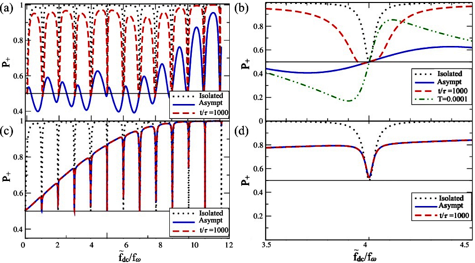
Figure 1: Population $P_{+}$ as a function of the $dc$ flux detuning ${\tilde{f}}_{dc}$ (normalized by $f_{\omega}=\omega_{0}/4\pi I_{p}$) for the FQ restricted to TLS, driven with amplitude $f_{ac}=0.003$ and $\omega_{0}=2\pi/\tau=0.003E_{J}/\hbar$. The Ohmic bath is at $T=0.0014$ ($20$mK for $E_{J}/h\approx 300{\rm GHz}$). Dotted line: $\overline{P}_{+}$ for the isolated system; solid line: $P_{+}(t=1000\tau)$, dashed line: asymptotic ($t\rightarrow\infty$) $\overline{P}_{+}$. Horizontal solid line indicates $P_{+}=0.5$ value. (a) Longitudinal coupling for an Ohmic bath with $\gamma^{(f)}=0.001$ and (b) enlarged view of (a) around n=4 photon resonance. (c) Transverse coupling for an Ohmic bath with $\gamma^{(ch)}=0.001$ and (d) enlarged view of (c) around n=4 photon resonance.

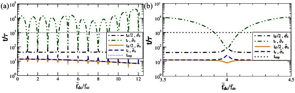
Figure 2: (a) Relaxation time $t_{r}$ for the longitudinal (dashed-double dotted line) and transverse (dashed line) couplings. (Half) decoherence time $t_{d}/2$ for the longitudinal (dashed-dotted line) and transverse (solid line) couplings. The flux detuning is normalized by $f_{\omega}=\omega_{0}/4\pi I_{p}$, such that the $n$-photon resonances are at ${\tilde{f}}=nf_{\omega}$. (b) Enlarged view of (a) around the $n=4$ resonance. The experimental time $t_{exp}/\tau=$ 1000 is plotted by the dotted line.

In Figs.1(a-b) and Figs.1(c-d) we plot $P_{+}$ for longitudinal and transverse couplings respectively, as a function of the flux detuning ${\tilde{f}}_{dc}$ for a fixed value of $f_{ac}=0.003$. As a comparison, for both couplings we plot $\overline{P}_{+}$ for the isolated case (without dissipation), where the $n$-photon resonances are clearly displayed as minima at $\epsilon_{0}/\omega_{0}={\tilde{f}}_{dc}/f_{\omega}=n$. For longitudinal coupling, Fig.1(a) shows that for time scales of FQ experiments Oliver et al. (2005) (we take here as a typical value $t_{exp}=1000\tau$), the behavior of $P_{+}$ is similar to the isolated case, with a broadening of the minima at the multiphoton resonances due to decoherence. On the other hand, in the asymptotic $t\rightarrow\infty$ steady state, $P_{+}$ exhibits antisymmetric multiphoton resonances Blattmann et al. (2015); Ferrón et al. (2016), clearly displayed in Fig.1(b), where an enlarged view around the $n=4$ resonance is shown. Morover, as the temperature is lowered, the antisymmetry around the resonance condition is more evident, as it is shown for $T=0.0001E_{J}/k_{B}$.

For transverse coupling, see Figs.1(c) and (d), the behavior of $P_{+}$ vs. ${\tilde{f}}_{dc}$ is remarkably different from the previous case: (i) there are no noticeable differences between the finite time and the steady sate $P_{+}$; (ii) the multiphoton resonances are symmetric in the steady state; (iii) there is no broadening of the resonances compared to the isolated case; and (iv) there is a linear background in $P_{+}$ as a function of ${\tilde{f}}_{dc}$ for the off-resonant situations. The hallmarks (ii) and (iv) have been also found in Ref.[Blattmann et al., 2015]. The linear background in $P_{+}$ can be understood by a simple argument. The transverse coupling through $\sigma_{y}$ provides a direct relaxation mechanism to the ground state (same holds for $\sigma_{x}$ coupling). Assuming that for the off-resonant situations in the steady state the qubit is fully relaxed in the ground state, we can estimate that in average is $P_{+}\sim t^{\prime}/\tau$, with $t^{\prime}$ the time scale within one period $\tau$ in which the ground state has nearly complete overlap with the $|+\rangle$ state (when ${\tilde{f}}(t)>0$). For small ${\tilde{f}}_{dc}/f_{ac}$ this gives $P_{+}\sim\frac{1}{2}+\frac{1}{\pi}\frac{{\tilde{f}}_{dc}}{f_{ac}}$. This straightforward calculation illustrates the linear background in the dependence of $P_{+}$ with $f_{dc}$ observed in Fig1(c).

The above described features have its correlation in the behaviour of the relaxation ($t_{r}$) and the decoherence ($t_{d}$) times, which are shown in Fig.2 for both types of couplings. They are calculated numerically from the eigenvalues of ${\Lambda}$ defined in Eq.(10), the maximum non-zero real eigenvalue of ${\Lambda}$ gives $-t_{r}^{-1}$, and the real part of the complex conjugates eigenvalues of ${\Lambda}$ give $-t_{d}^{-1}$ Ferrón et al. (2010, 2016). In general is $\frac{1}{t_{d}}=\frac{1}{2t_{r}}+\frac{1}{t_{\phi}}$ with $t_{\phi}$ the dephasing time and thus the decoherence time satisfies $t_{d}\leq 2t_{r}$ Grifoni and Hänggi (1998).

For the longitudinal coupling case we find in Fig.2 that the equality $t_{d}=2t_{r}$ is satisfied at the multiphoton resonances. Thus at the resonances the dephasing mechanism vanishes, similarly to what is usually found for the static case at the “sweet spot” $\tilde{f}=0$ Yan et al. (2016); Bylander et al. (2011). Away from resonances is $t_{d}\ll t_{r}$, showing a large time scale separation between decoherence and relaxation, due to strong dephasing. We have also obtained an analytic expression for the rates $\Gamma_{r}=1/t_{r}$ and the decoherence rate $\Gamma_{d}=1/t_{d}$ employing a RWA approximation for detunings near the $n$-photon resonance, $\tilde{f}\sim nf_{\omega}$, which are in good agreement with these numerical results (see the Appendix for a detailed calculation). In the case of longitudinal noise, the relaxation rates can be estimated as:

$$\Gamma_{{}_{r}} = |\lambda_{f}\sin(2\varphi)|^{2}[g(-\Omega_{n})+g(\Omega_{n})],$$

$$\Gamma_{d} = \frac{\Gamma_{r}}{2}+|\lambda_{f}\cos(2\varphi)|^{2}g(0),$$

with $\cos(2\varphi)=\epsilon_{n}/\varOmega_{n}$, $\sin(2\varphi)=\Delta_{-n}/\varOmega_{n}$, $\epsilon_{n}=4\pi I_{p}(\tilde{f}-nf_{\omega}$). The generalized Rabi frequency is $\varOmega_{n}=\sqrt{\epsilon_{n}^{2}+\Delta_{-n}^{2}}$ and $\Delta_{-n}=\Delta J_{-n}(x)$ with $x\equiv{f_{ac}/f_{\omega}}$. At the resonance is $\cos(2\varphi)=0$ and $\sin(2\varphi)=1$, thus $\Gamma_{d}=\Gamma_{r}/2$ and $\Gamma_{r}$ is maximum. Away from resonance the dephasing rate is maximum and $\Gamma_{\phi}=\Gamma_{d}-\Gamma_{r}/2\sim\lambda_{f}^{2}g(0)\approx\lambda_{f}^{2}\gamma kT$ (assuming $\cos(2\varphi)\sim 1$). This in agreement with the exact numerical results of Figures 2(a) and (b) where $t_{d}\ll t_{exp}\ll t_{r}$ away from resonance for the longitudinal case. This time scale separation allows the dynamic transition described in Ref.[Ferrón et al., 2016] and is also shown in Fig.3(a). We see that while $P_{+}$ remains symmetric around a resonance for $t_{d}<t<t_{r}$, there is a dynamic transition to the antisymmetric behavior for $t>t_{r}$.

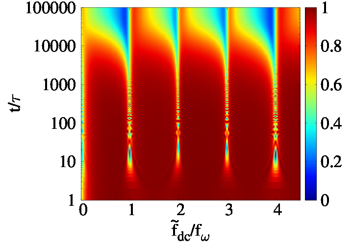
(a)

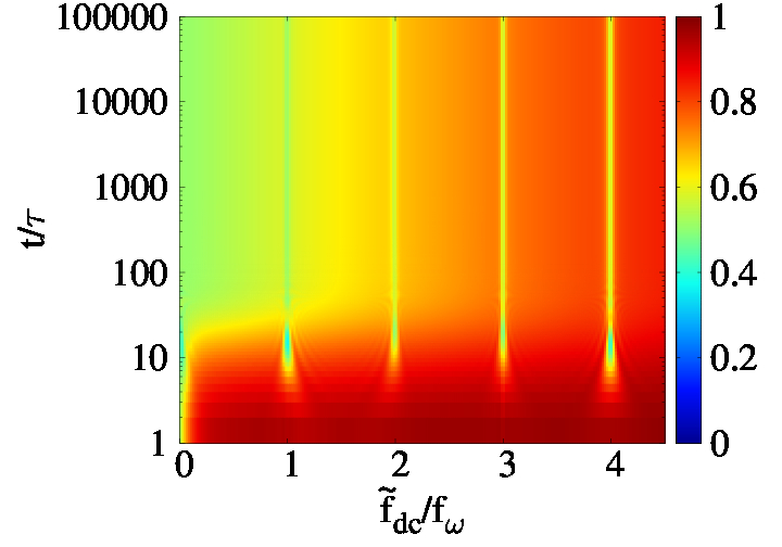
(b)

Figure 3: (color online) Intensity plots of the population $P_{+}$ as a function of ${\tilde{f}}_{dc}$ and driving time $t$. (a) Longitudinal coupling for $\gamma^{(f)}=0.001$. (b) Transverse coupling for $\gamma^{(ch)}=0.001$. See text for details.

On the other hand, for the transverse coupling case we find in Figs.2(a) and (b) that the equality $t_{d}=2t_{r}$ is reached out of resonance, i.e. opposite to the longitudinal case, while near the resonances the (small) dephasing gives $t_{d}\lesssim 2t_{r}$. The RWA calculation detailed in the Appendix is also consistent with this numerical result. For the transverse coupling we got:

$$\Gamma_{r} = |\lambda_{ch}J_{-n}(x)\cos(2\varphi)|^{2}[g(-\Omega_{n})+g(\Omega_{n})],$$

$$\Gamma_{d} = \frac{\Gamma_{r}}{2}+|\lambda_{ch}J_{-n}(x)\sin(2\varphi)|^{2}g(0).$$

In this case, away from resonance is $|\epsilon_{n}|\gg\Delta_{-n}$ implying $\sin(2\varphi)\sim 0$, $\cos(2\varphi)\sim 1$ and thus $\Gamma_{d}\approx\Gamma_{r}/2$. At a resonance the opposite condition is satisfied: the dephasing rate is maximum and thus $\Gamma_{\phi}\propto|\lambda_{ch}|^{2}g(0)\approx|\lambda_{ch}|^{2}\gamma kT$.

In addition, for transverse coupling the system tends to relax fast to the steady state in comparison to the longitudinal coupling case (assuming the same coupling strengths $\lambda^{\prime}s$). Note that, in the RWA calculation, out of resonance is $\cos 2\varphi^{2}\gg\sin 2\varphi^{2}$ and then $\Gamma_{r}^{\rm transverse}\gg\Gamma_{r}^{\rm longitudinal}$ for the same $\lambda$. This relatively fast relaxation is evident in Fig.3(b) where the steady state is quickly reached and no symmetry change around the resonance is observed.

II.3 Mixed noise

We deal now with the more general case when two sources of independent noise are taken into account, as formulated in Sec.I, and we consider the two system-bath couplings with ${\mathcal{A}}^{f}=-\lambda_{f}{\sigma}_{z}$ and ${\mathcal{A}}^{ch}=-\lambda_{ch}{\sigma}_{y}$. For simplicity we consider as before $J^{(f)}(\omega)=J^{(ch)}(\omega)=\gamma\omega e^{-\omega/\omega_{c}}$.

In order to compare the relative coupling strengths we define $\lambda_{f}=\cos\theta$ and $\lambda_{ch}=\sin\theta$. We plot in Fig.4 $P_{+}$ for $f_{ac}=0.003$, as a function of the mixing parameter $\cos^{2}\theta$ and ${\tilde{f}}_{dc}$, for the stationary case (Fig.4(a)) and for finite time $t=1000\tau$ (Fig.4(b)). In both cases the plots exhibit a behavior similar to the one obtained for the transverse coupling (see Fig.3(b)), for almost all the range of $\cos^{2}\theta$. Only when $(\lambda^{(ch)}/\lambda^{(f)})^{2}<0.005$ the typical features of the pure longitudinal case (already described) are observed.

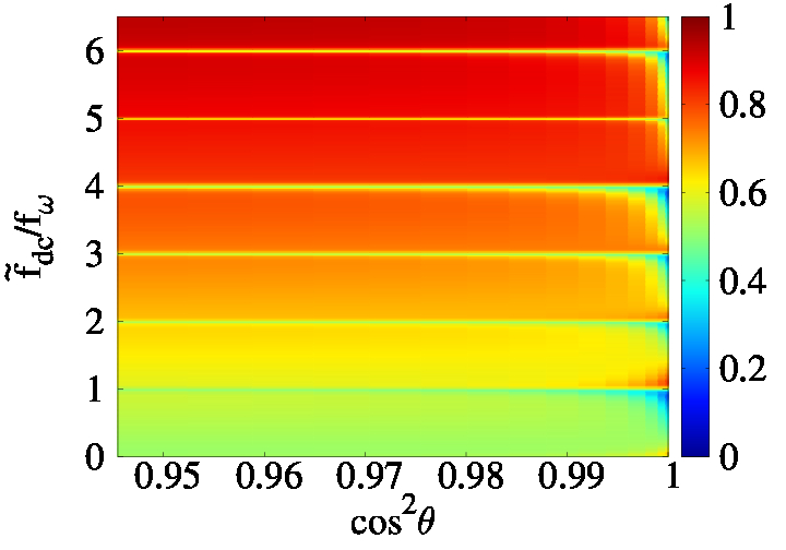
(a)

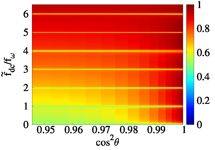
(b)

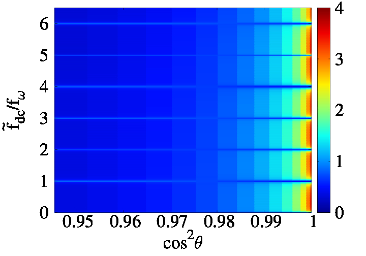
(c)

Figure 4: Intensity plots of the population $P_{+}$ as a function of ${\tilde{f}}_{dc}$ and the mixing parameter $\cos^{2}\theta$. $\gamma^{(f)}=\gamma\cos^{2}\theta$ and $\gamma^{(ch)}=\gamma\sin^{2}\theta$, with $\gamma=0.001$. (a) $t=\infty$, (b) $t=1000\tau$, (c) Intensity plot of the ratio of $\log({2t_{r}/t_{d}})$.

In agreement with the observed response in $P_{+}$, Fig.4(c) shows that $2t_{r}/t_{d}\sim 1$ for almost all the range of the mixing parameter, and only when approaching the longitudinal case, $(\lambda^{(ch)}/\lambda^{(f)})^{2}<0.005$, the time scale separation $2t_{r}/t_{d}\gg 1$ is observed in the off-resonant regions.

III Multilevel regime: LZS diamonds

The previous analysis can be extended to the multilevel regime which corresponds to realistic parameters of the FQ. We focus on the dynamics of the four lowest energy levels of the device, where the spectrum shows a rich structure of avoided crossings as a function of the dc detuning Oliver et al. (2005); Ferrón et al. (2010). We solve the Floquet-Markov equations for the Hamiltonian of Eq.(1), restricted to the subspace of spanned by the four lowest levels. Here we will compare the LZS patterns for pure flux noise and pure charge noise. In both cases we consider an Ohmic bath with spectral density $J(\omega)=\gamma\omega e^{-\omega/\omega_{c}}$ at temperature $T$, but different coupling operators. For pure flux (longitudinal) noise we take

$${\mathcal{A}}^{(flux)}=2\pi\alpha\sin(2\pi f+2\varphi_{m}),$$

which in the case of the two lowest levels subspace corresponds to ${\mathcal{A}}\approx-\lambda_{f}{\sigma}_{z}$, with $\lambda_{f}=2\pi\alpha|\langle+|\sin(2\pi f+2{\varphi}_{m})|+\rangle|\approx 4.5$, for FQ parameters $\alpha=0.8$ and $\eta=0.25$.

In the case of charge (transverse) noise the system operator is

$${\mathcal{A}}^{(charge)}={n}_{m}=i\frac{\eta^{2}}{2(1+2\alpha)}\frac{\partial}{\partial\varphi_{m}},$$

which for the two lowest levels subspace gives ${\mathcal{A}}\approx-\lambda_{ch}{\sigma}_{y}$, with $\lambda_{ch}=\frac{\eta^{2}}{4+8\alpha}|\langle-|{n}_{m}|+\rangle|\approx 3\times 10^{-4}$ for the same FQ parameters.

Notice that, after introducing realistic parameters, we obtain $\lambda_{ch}\ll\lambda_{f}$. For this parameter values, since $(\lambda^{(ch)}/\lambda^{(f)})^{2}\sim 10^{-8}\ll 0.005$, it is irrelevant to study the mixed dynamics with both types of couplings since the transverse noise effects will be unobserved. Thus, we will consider only the cases of pure longitudinal and pure transverse noise in this section to analyze the effect of each type of noise on the LZS patterns separately.

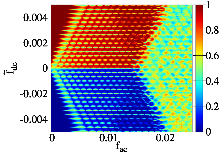
(a)

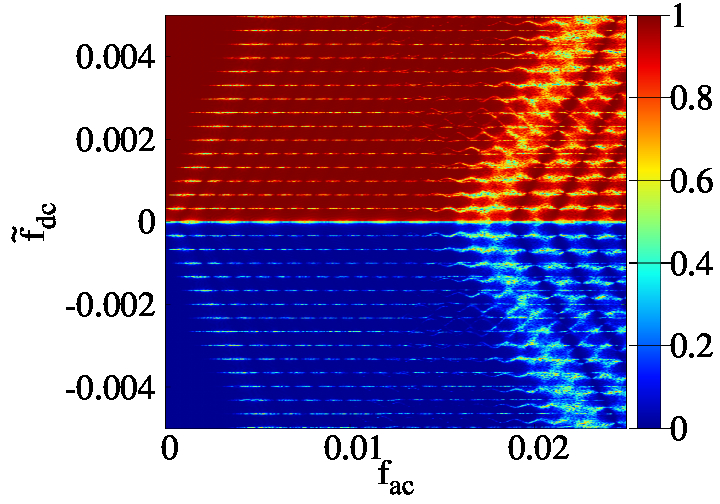
(b)

Figure 5: LZS interference patterns. Plots of $P_{+}$ as a function of the driving amplitude $f_{ac}$ and dc detuning ${\tilde{f}}_{dc}$ for $t=1000\tau$. (a) Flux noise. (b) Charge noise. The calculations were performed for $\omega_{0}=2\pi/\tau=0.003E_{J}/\hbar$, Ohmic bath at $T=0.0014E_{J}/k_{B}\sim 20$mK and $\gamma=0.001$ (see text for details).

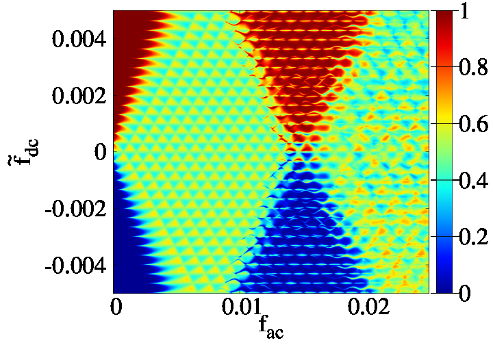
(a)

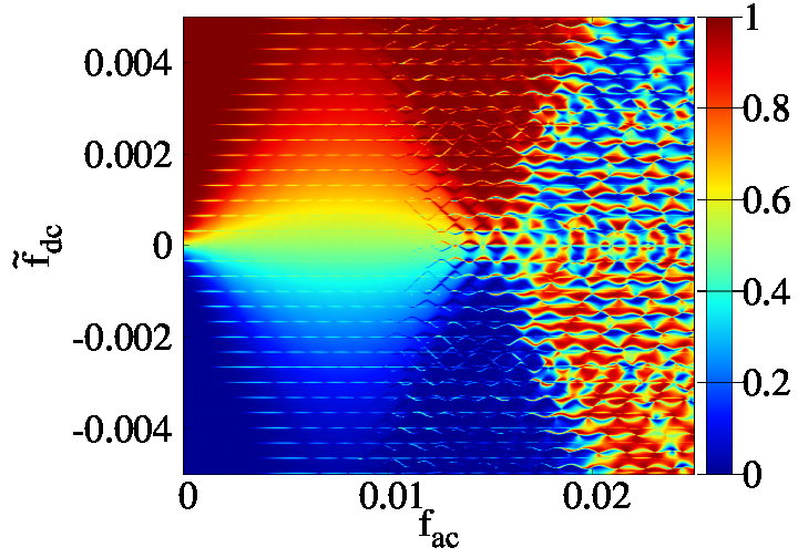
(b)

Figure 6: LZS interference patterns. Plots of $P_{+}$ as a function of the driving amplitude $f_{ac}$ and dc detuning ${\tilde{f}}_{dc}$ for the asymptotic regime, $t\rightarrow\infty$. (a) Flux noise. (b) Charge noise. Same parameters as in Fig.(5).

In Fig.5 we plot $P_{+}$ as a function of the driving amplitude $f_{ac}$ and dc detuning ${\tilde{f}}_{dc}$, for $t_{exp}=1000\tau$ and in Fig.6 for the steady state. The LZS interference patterns show the typical ”diamonds” structure for increasing $f_{ac}$, concomitant with the additional transitions at the avoided crossings between different energy levels Berns et al. (2008); Ferrón et al. (2012, 2016). We plot a range of $f_{ac}$ that shows the first LZS diamond, D1, and the lower half of the second LZS diamond, D2. D1 can be described in terms of the dynamics of the two lowest energy levels, the region between D1 and D2 involves the dynamics of the three lowest energy levels; while D2 includes the four lowest energy levels (see Ref.[Berns et al., 2008] for a complete description of the multilevel LZS diamonds).

For finite time $t\sim t_{exp}$, symmetric resonance lobes are observed within D1 for both types of coulpling. However, for the transverse coupling case (Fig.5(b)) the resonance lobes are narrower than for the longitudinal coupling (Fig.5(a)). The width of the resonance peaks is roughly proportional to the decoherence rate $1/t_{d}$ Shevchenko et al. (2010); Oliver et al. (2005). As analyzed in the previous section, in the transverse case dephasing mechanisms vanish out of resonance and $1/t_{d}$ is minimum. On the other hand, the dephasing rate grows out of resonance in the longitudinal case, and $1/t_{d}$ is large.

In the steady state the differences among the two types of coupling are stronger. While for the longitudinal coupling, Fig.6(a) shows the triangular checkerboard pattern characteristic of antisymmetric resonances together with population inversion (both features described in detail in Refs.Ferrón et al. (2012, 2016)), for the transverse coupling (Fig.6(b)), D1 exhibits a predominant background with a symmetric lobe in $P_{+}$ around $\tilde{f_{dc}}=0$. Within D2 and for the longitudinal coupling case, the patterns look qualitatively similar at finite time $t\sim t_{exp}$ and in the steady state, respectively. On the other hand, for the transverse coupling case, the steady state profile shows a strong population inversion in D2, absent at finite time $t\sim t_{exp}$.

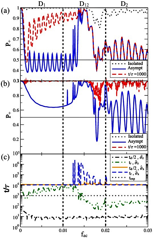
Figure 7: $P_{+}$ vs $f_{ac}$ for $\tilde{f}_{dc}\equiv 2.7f_{\omega}$, for $t=1000\tau$ (red dashed line), asymptotic state, $t\rightarrow{\infty}$, (blue solid line) and for the isolated case (dots). (a) Flux noise. (b) Charge noise. (c) $t_{r}/\tau$ for flux noise (dashed-double dotted line) and charge noise (dashed line). ${t_{d}}/2\tau$ for flux noise (dot-solid line) and charge noise (solid line). $t_{exp}=1000\tau$ (dotted line). Vertical dashed lines are guides for the eyes to show the boundaries of diamonds D1, D2 and the region in between, named D12, for the value of $\tilde{f}_{dc}\equiv 2.7f_{\omega}$.

To understand the different time scales, we plot $P_{+}$ at a finite time and in the steady state, as a function of the driving amplitude $f_{ac}$ for a fixed off-resonant value of detuning $\tilde{f}_{dc}=0.0009\equiv 2.7f_{\omega}$, for the the longitudinal coupling (Fig.7(a)) and for the transverse coupling (Fig.7(b)), respectively. The time scales of decoherence and relaxation, $t_{d}$ and $t_{r}$, are plotted in Fig.7(c). In the previous section we concluded that for same coupling strengths, $\lambda_{ch}=\lambda_{f}$, the transverse coupling leads to a faster relaxation rate. Here, the smallness of $\lambda_{ch}$ gives a much larger $t_{r}$ than in the $\lambda_{ch}\sim 1$ case analyzed previously. It is interesting to note in Fig.7(c) that the resulting $t_{r}$ for the transverse coupling turns out to be of the same order or larger than in the longitudinal case.

From Fig.7(c) it follows that for the longitudinal case and within D1, there is a large time scale separation $t_{d}\ll t_{exp}\ll t_{r}$, in agreement with the different behaviors of $P_{+}(t_{exp}=1000\tau)$ and $P_{+}(\infty)$ seen in Fig.7(a). The relaxation time strongly depends on $f_{ac}$ and within D2, $t_{r}$ is reduced two orders of magnitude, leading to $t_{r}<t_{exp}$ and therefore $P_{+}(t_{exp})\approx P_{+}(\infty)$.

For the transverse coupling case, see Fig.7(b), within both diamonds D1 and D2 the time scales $t_{r}$ and $t_{d}$ are both larger than $t_{exp}=1000\tau$ and nearly independent of $f_{ac}$ (except in the transition between D1 and D2). Thus, for this type of coupling the steady state behavior could not be seen at the experimental time scale neither for D1 nor for D2. Furthermore, it is also evident that the decoherence rate is minimum since $t_{r}\sim t_{d}/2$ in all the range of $f_{ac}$, even beyond the two level regime discussed in the previous section.

From our analysis it is clear that the experimental results of Refs.[Oliver et al. (2005); Oliver and Valenzuela (2009)] do not correspond to any of the steady state LSZ patterns of Fig.6, since these experiments do not show neither the anstisymmetric resonance patterns of the longitudinal coupling nor the background lobe for off-resonant population of the transverse coupling. In addition, the extremely narrow resonance lobes of Fig.5(b) for the transverse coupling do not seem to represent well the experimental data. The symmetric resonance lobes of the experimental LZS patterns are more in agreement with the case of Fig.5(a) for longitudinal coupling. This conclusion is consistent with the noise spectroscopy measurements of Refs.Bylander et al. (2011); Yan et al. (2013); Yoshihara et al. (2014) that found that the transverse noise is very small for FQ devices.

IV Concluding Remarks

We have performed a systematic analysis of environmental noise effects for a strongly driven FQ device, considering a realistic multilevel dynamics and emphasizing the behavior at different time scales.

A main outcome of our work is to expose the LZS interferometry as a tool to unveil the type of system-bath coupling, where the presence of symmetric (asymmetric) n-photon resonances in the stationary patterns reveals the nature of the noise, i.e. transverse (longitudinal) system-bath coupling.

In addition the analysis of the relaxation and decoherence time scales shows that the ratio $t_{r}/2t_{d}$ is also extremely sensitive to the type of system-bath coupling and might change significantly when a n-photon resonance is tuned.

For time scales prior to relaxation, the LZS interferometric patterns also exhibit two well differentiated behaviours depending on the noise sources. Along this line, our results for the FQ device in the regime of strong driving (beyond the TLS regime) shed light on the interpretation of the experimental LZS diamonds obtained in Ref.Berns et al. (2008); Oliver and Valenzuela (2009) for a driven FQ with long relaxation times. The symmetric resonances lobes observed in Ref.Berns et al. (2008); Oliver and Valenzuela (2009) are in agreement with the longitudinal noise scenario shown in Fig.5(a). However, to conclusively discard other possible scenarios, experiments should be performed for larger driving times, in order to reach the steady state after full relaxation with the bath degrees of freedom.

Experimental studies of noise spectroscopy for the FQ, when driven at the first resonance, have shown that flux noise is the dominant source of decoherenceYan et al. (2013); Yoshihara et al. (2014). This result is also consistent with the scenario of longitudinal noise found in Fig.5(a) for the case of multiphoton resonances and large amplitudes. However, flux noise power spectrum at low frequencies has shown $1/f$ behavior Bylander et al. (2011); Yan et al. (2013); Yoshihara et al. (2014). Thus, to better account noise effects in the steady state or long time limit, future studies based on a non-markovian description Stace et al. (2013) would be interesting.

Even when we have considered specific parameters of the FQ, our results can be also useful for other qubits and artificial atoms devices, in which the amplitude spectroscopy technique based on LZS interferometry has been implemented during the last years Sillanpää et al. (2006); Mark et al. (2007); Wilson et al. (2010); Petta et al. (2010); Kling et al. (2010); Huang et al. (2011).

We acknowledge financial support from CNEA, CONICET (PIP11220150100756), UNCuyo (P 06/C455) and ANPCyT (PICT2014-1382, PICT2016-0791).

Appendix A The rotating wave approximation: dressed basis

In this section we briefly revisit the Rotating Wave Approximation (RWA) applied to multiphoton resonances Wilson et al. (2007); Ashhab et al. (2007); Shevchenko et al. (2010); Kmetic M. A. and J. (1986). We start by considering the general Two Level System (TLS) Hamiltonian:

$${\mathcal{H}}_{TLS}(t)=-\frac{\epsilon(t)}{2}{\sigma}_{z}-\frac{\Delta}{2}{\sigma}_{x}$$ (13)

where $\epsilon(t)=\epsilon_{0}+A\cos(\omega_{0}t)$. The parameter $\epsilon_{0}$ is the polarization energy of the qubit, $A$ and $\omega$ the amplitude and frequency of the driving, respectively. By applying the unitary transformation $|\tilde{\psi}(t)\rangle=U_{\phi}(t)|\psi(t)\rangle$, with $U_{\phi}(t)=e^{-i\frac{\phi(t)}{2}{\sigma}_{z}}$ and $\phi(t)=\int\epsilon(t)\,dt=\epsilon_{0}t+A/\omega_{0}\sin(\omega_{0}t)$, the transformed Hamiltonian reads:

$${\tilde{H}}=-\frac{(\epsilon-\dot{\phi}(t))}{2}{\sigma}_{z}-\frac{\Delta}{2}(e^{-i\phi(t)}{\sigma}_{+}+h.c).$$ (14)

Replacing $\phi(t)\rightarrow\phi_{n}(t)=n\omega_{0}t+\frac{A}{\omega_{0}}\sin\omega_{0}t$ (which is equivalent to take the resonance condition $\epsilon_{0}\sim n\omega_{0}$) the Hamiltonian transforms to:

$${\tilde{H}}=-\frac{(\epsilon_{0}-n\omega_{0})}{2}{\sigma}_{z}-\frac{\Delta}{2}(e^{-in\omega_{0}t}e^{-i\frac{A}{\omega_{0}}\sin\omega_{0}t}{\sigma}_{+}+h.c).$$ (15)

Using in addition that $e^{ix\sin a}=\sum_{k=-\infty}^{k=+\infty}J_{k}(x)e^{ika}$, with $J_{k}(x)$ the Bessel function of order $k$, we can write:

$$e^{in\omega_{0}t}e^{i\frac{A}{\omega_{0}}\sin\omega_{0}t}=\sum_{k=-\infty}^{k=+\infty}J_{k}(\frac{A}{\omega_{0}})e^{i(k+n)\omega_{0}t}\simeq J_{-n}(\frac{A}{\omega_{0}})$$ (16)

where in the last step we have performed a rotating wave approximation (RWA), for $|\epsilon_{0}-n\omega_{0}|\ll\varDelta$. In this way, we finally obtain the TLS Hamiltonian written in the RWA as:

$${\tilde{H}}\simeq{\tilde{H}}_{n}=-\frac{(\epsilon_{0}-n\omega_{0})}{2}{\sigma}_{z}-\frac{\Delta_{-n}}{2}{\sigma}_{x},$$ (17)

with $\Delta_{-n}=\Delta J_{-n}(\frac{A}{\omega_{0}})$.

Notice that after the RWA we have obtained an effective time-independent “dressed” Hamiltonian. Going a step further, we proceed to diagonalize ${\tilde{H}}_{n}$ considering the operator $U_{r}=\cos(\varphi){\sigma}_{z}+\sin(\varphi){\sigma}_{x}$. After applying such transformation, we finally obtain the “dressed” Hamiltonian

$${{H}}_{r}=U_{r}{\tilde{H}}_{n}U_{r}^{-1}=-\frac{\varOmega_{n}}{2}{\sigma}_{z},$$ (18)

with $\cos(2\varphi)=\epsilon_{n}/\varOmega_{n}$, $\sin(2\varphi)=\Delta_{-n}/\varOmega_{n}$, $\epsilon_{n}=\epsilon_{0}-n\omega_{0}$, and $\varOmega_{n}=\sqrt{(\epsilon_{0}-n\omega_{0})^{2}+\Delta_{-n}^{2}}$ the generalized Rabi frequency. It is worth noting that the eigenenergies of ${H}_{r}$ exhibit an avoided crossing with an effective “dressed” gap $\Delta_{-n}$, and the associated eigenstates form the “dressed” basis.

Appendix B Calculation of relaxation and decoherence rates in the rotating wave approximation

The dynamics of an open system can be described by the total Hamiltonian:

$$H_{T}(t)={\mathcal{H}}_{TLS}(t)+H_{B}+{H}_{int},$$ (19)

where ${\mathcal{H}}_{TLS}(t)$ is the driven TLS Hamiltonian, $H_{B}$ the bath term and

$${H}_{int}={\mathcal{A}}\otimes{\mathcal{B}},$$ (20)

the system-bath interaction term. In the present analysis the system operator, ${\mathcal{A}}$, can be ${\mathcal{A}}_{z}=\lambda_{z}{\sigma}_{z}$ or ${\mathcal{A}}_{x}=\lambda_{x}{\sigma}_{x}$ and ${\mathcal{B}}$ is the bath operator.

The von Neumann equation for time-evolution of the system described by the total Hamiltonian (19) is ((taking $\hbar=1$)

$$\frac{\partial\rho_{T}(t)}{\partial t}=-i[H_{T}(t),\rho_{T}(t)],$$ (21)

with $\rho_{T}(t)$ the density matrix of the global system.

We start by defining $H_{0}(t)={\mathcal{H}}_{TLS}(t)+H_{B}$, and the associated evolution operator $U_{0}(t)=\hat{\mathcal{T}}e^{-i\int H_{0}(t)\,dt}$ . Therefore, in the Interaction Picture the transformed operators are ${\tilde{\rho}}(t)=U_{0}^{\dagger}(t)\rho(t)U_{0}(t)$ and ${\tilde{H}}_{int}(t)=U_{0}^{\dagger}(t){H}_{int}U_{0}(t)$, and Eq.(21) reads:

$$\frac{\partial{\tilde{\rho_{T}}}(t)}{\partial t}=-i[{\tilde{H}}_{int}(t),{\tilde{\rho_{T}}}(t)].$$ (22)

After defining the system reduced density matrix $\rho=Tr_{B}(\rho_{T})$ and performing the Born-Markov approximation, we get:

$$\frac{\partial{\tilde{\rho}}}{\partial t} = -\int_{0}^{\infty}dt^{\prime}\{G(t^{\prime})[{\tilde{\mathcal{A}}}(t){\tilde{\mathcal{A}}}(t-t^{\prime}){\tilde{\rho}}-{\tilde{\mathcal{A}}}(t-t^{\prime}){\tilde{\rho}}{\tilde{\mathcal{A}}}(t)]$$ (23)

$$+G(-t^{\prime})[{\tilde{\rho}}{\tilde{\mathcal{A}}}(t-t^{\prime}){\tilde{\mathcal{A}}}(t)-{\tilde{\mathcal{A}}}(t){\tilde{\rho}}{\tilde{\mathcal{A}}}(t-t^{\prime})],$$

with $G(t)=\mathrm{Tr}_{B}\Big{(}{\mathcal{B}}(t){\mathcal{B}}(0)\rho_{B}\Big{)}$ the bath correlation function and ${\tilde{\mathcal{A}}}(t)=U_{0}^{\dagger}(t){\mathcal{A}}U_{0}(t)$.

Now, we set the decomposition

$${\tilde{\mathcal{A}}}(t)=\sum_{\omega}e^{-i\omega t}P_{\omega}=\sum_{\omega}e^{i\omega t}P_{\omega}^{\dagger}=\sum_{\omega>0}e^{-i\omega t}P_{\omega}+e^{i\omega t}P_{\omega}^{\dagger}$$ (24)

with $P_{-\omega}=P_{\omega}^{{\dagger}}$. Moreover, we can define $\Gamma(\omega)=\int_{0}^{\infty}dte^{-i\omega t}G(t)=\frac{1}{2}g(\omega)+is(\omega)$Breuer and Petruccione (2006).

After performing the secular approximation, Eq.(23) can be expressed in the Lindblad form as:

$$\frac{\partial{\tilde{\rho}}}{\partial t}=-i[H_{L},{\tilde{\rho}}]+\sum_{\omega}g(\omega)(P_{\omega}{\tilde{\rho}}P_{\omega}^{\dagger}-\frac{1}{2}\{P_{\omega}^{\dagger}P_{\omega},{\tilde{\rho}}\})$$ (25)

with the Hamiltonian

$$H_{L}=\sum_{\omega}s(\omega)P_{\omega}^{\dagger}P_{\omega}.$$ (26)

We now proceed to transform the system operator ${\mathcal{A}}$ into the “dressed” representation Wilson et al. (2007), ${\mathcal{A}}\rightarrow{\mathcal{A}}_{r}$. Following the procedure described previously, we perform the transformation ${\mathcal{A}}_{r}(t)=U_{r}U_{n}{\mathcal{A}}U_{n}^{-1}U_{r}^{-1}$, with $U_{r}=\cos(\varphi){\sigma}_{z}+\sin(\varphi){\sigma}_{x}$ and $U_{n}(t)=e^{-i\frac{1}{2}\phi_{n}(t){\sigma}_{z}}$. For a system operator of the form ${\mathcal{A}}=\lambda(\cos\theta{\sigma}_{z}+\sin\theta{\sigma}_{x})$, we obtain the transformed ${\mathcal{A}}_{r}$ as:

$${\mathcal{A}}_{r}(t)=a_{x}(t){\sigma}_{x}+a_{y}(t){\sigma}_{y}+a_{z}(t){\sigma}_{z},$$ (27)

with the coefficients $a_{i}(t)$, $i=x,y,z$, satisfying the following relations:

$$a_{x}(t) = a_{x0}+a_{xc}\cos\phi_{n}(t)\approx a_{x0}+a_{xc}c_{0},$$

$$a_{y}(t) = a_{ys}\sin\phi_{n}(t)\approx 0,$$

$$a_{z}(t) = a_{z0}+a_{zc}\cos\phi_{n}(t)\approx a_{z0}+a_{zc}c_{0},$$

with $a_{x0}=\lambda\cos\theta\sin 2\varphi$, $a_{xc}=-\lambda\sin\theta\cos 2\varphi$, $a_{ys}=-\lambda\sin\theta$, $a_{z0}=\lambda\cos\theta\cos 2\varphi$ and $a_{zc}=\lambda\sin\theta\sin 2\varphi$. In the last step we have performed the RWA as in Eq.(16), with $c_{0}=J_{-n}(\frac{A}{\omega_{0}})$.

Transforming ${\mathcal{A}}_{r}$ to the Interaction picture one gets:

$${\tilde{\mathcal{A}}}_{r}(t)= (a_{x0}+a_{xc}c_{0})e^{i\Omega_{n}t}{\sigma}_{+}+(a_{x0}+a_{xc}c_{0})e^{-i\Omega_{n}t}{\sigma}_{-}$$ (28)

$$+(a_{z0}+a_{zc}c_{0}){\sigma}_{z},$$

To obtain the Linblad equation, we rewrite the above equation in terms of the decomposition of Eq.(24),

$${\tilde{\mathcal{A}}}_{r}(t) =P_{+}({\Omega_{n}})e^{i\Omega_{n}t}+P_{-}(-{\Omega_{n}})e^{-i\Omega_{n}t}+P_{0},$$ (29)

$$=P_{+}({\Omega_{n}})e^{i\Omega_{n}t}+P^{{\dagger}}_{+}({\Omega_{n}})e^{-i\Omega_{n}t}+P_{0},$$

$$=\sum_{\omega}P_{\omega}e^{i\omega t},$$

with $\omega\in\{0,{\Omega_{n}},-{\Omega_{n}}\}$ and $P_{\omega}=\{P_{z}(0),P_{+}({\Omega_{n}}),P_{-}(-{\Omega_{n}})\}\equiv\{P_{z}(0),P_{+}({\Omega_{n}}),P^{{\dagger}}_{+}({\Omega_{n}})\}$. The operators $P_{\omega}$ are:

$$P_{z}(0)= (a_{z0}+a_{zc}c_{0}){\sigma}_{z}=z(0){\sigma}_{0},$$ (30)

$$P_{+}({\Omega_{n}})= (a_{x0}+a_{xc}c_{0}){\sigma}_{+}=x(\Omega_{n}){\sigma}_{+},$$

$$P_{-}({-\Omega_{n}})= P^{{\dagger}}_{+}({\Omega_{n}})=x(-\Omega_{n}){\sigma}_{-},$$

with $z(0)=a_{z0}+a_{zc}c_{0}$ and $x({\Omega_{n}})=a_{x0}+a_{xc}c_{0}$.

Using Eq.(30) in Eq.(28), we obtain the Lindblad equation

$$\frac{\partial{\tilde{\rho}}}{\partial t}= -\Gamma_{\uparrow}\left(\begin{array}[]{cc}-{\tilde{\rho}}_{11}&\frac{1}{2}{\tilde{\rho}}_{12}\\ \frac{1}{2}{\tilde{\rho}}_{21}&{\tilde{\rho}}_{11}\end{array}\right)-\Gamma_{\downarrow}\left(\begin{array}[]{cc}{\tilde{\rho}}_{22}&\frac{1}{2}{\tilde{\rho}}_{12}\\ \frac{1}{2}{\tilde{\rho}}_{21}&-{\tilde{\rho}}_{22}\end{array}\right)$$ (31)

$$-\Gamma_{0}\left(\begin{array}[]{cc}0&{\tilde{\rho}}_{12}\\ {\tilde{\rho}}_{21}&0\end{array}\right)$$

with

$$\Gamma_{\uparrow} =|x(\Omega_{n})|^{2}g(-\Omega_{n})$$ (32)

$$\Gamma_{\downarrow} =|x(\Omega_{n})|^{2}g(\Omega_{n})$$

$$\Gamma_{o} =|z(0)|^{2}g(0)$$

After solving Eq.(31), the relaxation $\Gamma_{r}$ and decoherence $\Gamma_{d}$ rates can be computed as

$$\Gamma_{d} =\Gamma_{\downarrow}+\Gamma_{\uparrow},$$ (33)

$$\Gamma_{r} =\Gamma_{0}+\frac{\Gamma_{d}}{2}.$$

Considering the system-bath coupling term ${\mathcal{A}}_{z}=\lambda_{z}\sigma_{z}$, the rates in Eq.(33) take the form

$$\Gamma^{z}_{\uparrow} =|\lambda_{z}\sin(2\varphi)|^{2}g(-\Omega_{n}),$$ (34)

$$\Gamma^{z}_{\downarrow} =|\lambda_{z}\sin(2\varphi)|^{2}g(\Omega_{n}),$$

$$\Gamma^{z}_{o} =|\lambda_{z}\cos(2\varphi)|^{2}g(0).$$

Followed by

$$\Gamma^{z}_{d} =|\lambda_{z}\sin(2\varphi)|^{2}\Big{(}g(-\Omega_{n})+g(\Omega_{n})\Big{)},$$ (35)

$$\Gamma^{z}_{r} =|\lambda_{z}\cos(2\varphi)|^{2}g(0)+\frac{\Gamma^{z}_{d}}{2}.$$

For the ${\mathcal{A}}_{x}=\lambda_{x}\sigma_{x}$ case, the rates are

$$\Gamma^{x}_{\uparrow} =|\lambda_{x}c_{0}\cos(2\varphi)|^{2}g(-\Omega_{n})$$ (36)

$$\Gamma^{x}_{\downarrow} =|\lambda_{x}c_{0}\cos(2\varphi)|^{2}g(\Omega_{n})$$

$$\Gamma^{x}_{o} =|\lambda_{x}c_{0}\sin(2\varphi)|^{2}g(0).$$

For this case, the calculation of the rates $\Gamma^{x}_{d}$ and $\Gamma^{x}_{r}$ are rather cumbersome. We obtain:

$$\Gamma^{x}_{d}= |\lambda_{x}c_{0}\cos(2\varphi)|^{2}\Big{(}g(-\Omega_{n})+g(\Omega_{n})\Big{)}$$ (37)

$$\Gamma^{x}_{r}= |\lambda_{x}c_{0}\sin(2\varphi)|^{2}g(0).$$

In this way, we have extended the calculation of relaxation rates given in the Supplementary Information of Yan et al. (2013) to the case of $n$-photon resonances.

References

- Orlando et al. (1999) T. P. Orlando, J. E. Mooij, L. Tian, C. H. van der Wal, L. S. Levitov, S. Lloyd, and J. J. Mazo, Phys. Rev. B 60, 15398 (1999).
- Chiorescu et al. (2003) I. Chiorescu, Y. Nakamura, C. J. P. M. Harmans, and J. E. Mooij, Science 299, 1869 (2003), https://science.sciencemag.org/content/299/5614/1869.full.pdf .
- You and Nori (2011) J. Q. You and F. Nori, Nature 474, 589 EP (2011).
- Makhlin et al. (2001) Y. Makhlin, G. Schön, and A. Shnirman, Rev. Mod. Phys. 73, 357 (2001).
- Shevchenko et al. (2010) S. Shevchenko, S. Ashhab, and F. Nori, Physics Reports 492, 1 (2010).
- Oliver et al. (2005) W. D. Oliver, Y. Yu, J. C. Lee, K. K. Berggren, L. S. Levitov, and T. P. Orlando, Science 310, 1653 (2005), https://science.sciencemag.org/content/310/5754/1653.full.pdf .
- Berns et al. (2006) D. M. Berns, W. D. Oliver, S. O. Valenzuela, A. V. Shytov, K. K. Berggren, L. S. Levitov, and T. P. Orlando, Phys. Rev. Lett. 97, 150502 (2006).
- Berns et al. (2008) D. M. Berns, M. S. Rudner, S. O. Valenzuela, K. K. Berggren, W. D. Oliver, L. S. Levitov, and T. P. Orlando, Nature 455, 51 EP (2008).
- Oliver and Valenzuela (2009) W. D. Oliver and S. O. Valenzuela, Quantum Information Processing 8, 261 (2009).
- Izmalkov et al. (2008) A. Izmalkov, S. H. W. van der Ploeg, S. N. Shevchenko, M. Grajcar, E. Il’ichev, U. Hübner, A. N. Omelyanchouk, and H.-G. Meyer, Phys. Rev. Lett. 101, 017003 (2008).
- Sillanpää et al. (2006) M. Sillanpää, T. Lehtinen, A. Paila, Y. Makhlin, and P. Hakonen, Phys. Rev. Lett. 96, 187002 (2006).
- Wilson et al. (2007) C. M. Wilson, T. Duty, F. Persson, M. Sandberg, G. Johansson, and P. Delsing, Phys. Rev. Lett. 98, 257003 (2007).
- Yoakum et al. (1992) S. Yoakum, L. Sirko, and P. M. Koch, Phys. Rev. Lett. 69, 1919 (1992).
- Mark et al. (2007) M. Mark, T. Kraemer, P. Waldburger, J. Herbig, C. Chin, H.-C. Nägerl, and R. Grimm, Phys. Rev. Lett. 99, 113201 (2007).
- Kling et al. (2010) S. Kling, T. Salger, C. Grossert, and M. Weitz, Phys. Rev. Lett. 105, 215301 (2010).
- Huang et al. (2011) P. Huang, J. Zhou, F. Fang, X. Kong, X. Xu, C. Ju, and J. Du, Phys. Rev. X 1, 011003 (2011).
- Forster et al. (2014) F. Forster, G. Petersen, S. Manus, P. Hänggi, D. Schuh, W. Wegscheider, S. Kohler, and S. Ludwig, Phys. Rev. Lett. 112, 116803 (2014).
- Blattmann et al. (2015) R. Blattmann, P. Hänggi, and S. Kohler, Phys. Rev. A 91, 042109 (2015).
- Mi et al. (2018) X. Mi, S. Kohler, and J. R. Petta, Phys. Rev. B 98, 161404 (2018).
- Yan et al. (2016) F. Yan, S. Gustavsson, A. Kamal, J. Birenbaum, A. P. Sears, D. Hover, T. J. Gudmundsen, D. Rosenberg, G. Samach, S. Weber, J. L. Yoder, T. P. Orlando, J. Clarke, A. J. Kerman, and W. D. Oliver, Nature Communications 7, 12964 EP (2016).
- Bylander et al. (2011) J. Bylander, S. Gustavsson, F. Yan, F. Yoshihara, K. Harrabi, G. Fitch, D. G. Cory, Y. Nakamura, J.-S. Tsai, and W. D. Oliver, Nature Physics 7, 565 EP (2011).
- Yan et al. (2013) F. Yan, S. Gustavsson, J. Bylander, X. Jin, F. Yoshihara, D. G. Cory, Y. Nakamura, T. P. Orlando, and W. D. Oliver, Nature Communications 4, 2337 EP (2013).
- Yoshihara et al. (2014) F. Yoshihara, Y. Nakamura, F. Yan, S. Gustavsson, J. Bylander, W. D. Oliver, and J.-S. Tsai, Phys. Rev. B 89, 020503 (2014).
- Grifoni and Hänggi (1998) M. Grifoni and P. Hänggi, Physics Reports 304, 229 (1998).
- Kohler et al. (1998) S. Kohler, R. Utermann, P. Hänggi, and T. Dittrich, Phys. Rev. E 58, 7219 (1998).
- Hartmann et al. (2000) L. Hartmann, I. Goychuk, M. Grifoni, and P. Hänggi, Phys. Rev. E 61, R4687 (2000).
- Dakhnovskii et al. (1995) Y. Dakhnovskii, D. G. Evans, H. J. Kim, and R. D. Coalson, The Journal of Chemical Physics 103, 5461 (1995), https://doi.org/10.1063/1.470530 .
- Stace et al. (2005) T. M. Stace, A. C. Doherty, and S. D. Barrett, Phys. Rev. Lett. 95, 106801 (2005).
- Goorden et al. (2004) M. C. Goorden, M. Thorwart, and M. Grifoni, Phys. Rev. Lett. 93, 267005 (2004).
- Hausinger and Grifoni (2010) J. Hausinger and M. Grifoni, Phys. Rev. A 81, 022117 (2010).
- Ferrón et al. (2012) A. Ferrón, D. Domínguez, and M. J. Sánchez, Phys. Rev. Lett. 109, 237005 (2012).
- Ferrón et al. (2016) A. Ferrón, D. Domínguez, and M. J. Sánchez, Phys. Rev. B 93, 064521 (2016).
- Ferrón and Domínguez (2010) A. Ferrón and D. Domínguez, Phys. Rev. B 81, 104505 (2010).
- You et al. (2007) J. Q. You, X. Hu, S. Ashhab, and F. Nori, Phys. Rev. B 75, 140515 (2007).
- Sete et al. (2017) E. A. Sete, M. J. Reagor, N. Didier, and C. T. Rigetti, Phys. Rev. Applied 8, 024004 (2017).
- (36) For the qubit parameters under consideration, one can show that the ratio of matrix elements of the charge operators for the lowest energy states is . .
- Rudner et al. (2008) M. S. Rudner, A. V. Shytov, L. S. Levitov, D. M. Berns, W. D. Oliver, S. O. Valenzuela, and T. P. Orlando, Phys. Rev. Lett. 101, 190502 (2008).
- Shirley (1965) J. H. Shirley, Phys. Rev. 138, B979 (1965).
- Breuer et al. (2000) H.-P. Breuer, W. Huber, and F. Petruccione, Phys. Rev. E 61, 4883 (2000).
- Hone et al. (2009) D. W. Hone, R. Ketzmerick, and W. Kohn, Phys. Rev. E 79, 051129 (2009).
- Ferrón et al. (2010) A. Ferrón, D. Domínguez, and M. J. Sánchez, Phys. Rev. B 82, 134522 (2010).
- Ashhab et al. (2007) S. Ashhab, J. R. Johansson, A. M. Zagoskin, and F. Nori, Phys. Rev. A 75, 063414 (2007).
- Goorden, M. C. et al. (2005) Goorden, M. C., Thorwart, M., and Grifoni, M., Eur. Phys. J. B 45, 405 (2005).
- van der Wal, C. H. et al. (2003) van der Wal, C. H., Wilhelm, F. K., Harmans, C. J.P.M., and Mooij, J. E., Eur. Phys. J. B 31, 111 (2003).
- (45) Notice that when the different noise sources are fully correlated, such that , it is straightforward to show (after redefining ) that , i.e. there is an effective single noise source .
- Grossmann et al. (1991) F. Grossmann, T. Dittrich, P. Jung, and P. Hänggi, Phys. Rev. Lett. 67, 516 (1991).
- Kayanuma and Saito (2008) Y. Kayanuma and K. Saito, Phys. Rev. A 77, 010101 (2008).
- Wilson et al. (2010) C. M. Wilson, G. Johansson, T. Duty, F. Persson, M. Sandberg, and P. Delsing, Phys. Rev. B 81, 024520 (2010).
- Sun et al. (2009) G. Sun, X. Wen, Y. Wang, S. Cong, J. Chen, L. Kang, W. Xu, Y. Yu, S. Han, and P. Wu, Applied Physics Letters 94, 102502 (2009), https://doi.org/10.1063/1.3093823 .
- Sun et al. (2011) G. Sun, X. Wen, B. Mao, Y. Yu, J. Chen, W. Xu, L. Kang, P. Wu, and S. Han, Phys. Rev. B 83, 180507 (2011).
- Wang et al. (2010) Y. Wang, S. Cong, X. Wen, C. Pan, G. Sun, J. Chen, L. Kang, W. Xu, Y. Yu, and P. Wu, Phys. Rev. B 81, 144505 (2010).
- de Graaf et al. (2013) S. E. de Graaf, J. Leppäkangas, A. Adamyan, A. V. Danilov, T. Lindström, M. Fogelström, T. Bauch, G. Johansson, and S. E. Kubatkin, Phys. Rev. Lett. 111, 137002 (2013).
- Shevchenko et al. (2012) S. N. Shevchenko, A. N. Omelyanchouk, and E. Il’ichev, Low Temperature Physics 38, 283 (2012), https://doi.org/10.1063/1.3701717 .
- Petta et al. (2010) J. R. Petta, H. Lu, and A. C. Gossard, Science 327, 669 (2010), https://science.sciencemag.org/content/327/5966/669.full.pdf .
- Stehlik et al. (2012) J. Stehlik, Y. Dovzhenko, J. R. Petta, J. R. Johansson, F. Nori, H. Lu, and A. C. Gossard, Phys. Rev. B 86, 121303 (2012).
- Cao et al. (2013) G. Cao, H.-O. Li, T. Tu, L. Wang, C. Zhou, M. Xiao, G.-C. Guo, H.-W. Jiang, and G.-P. Guo, Nature Communications 4, 1401 EP (2013).
- Dupont-Ferrier et al. (2013) E. Dupont-Ferrier, B. Roche, B. Voisin, X. Jehl, R. Wacquez, M. Vinet, M. Sanquer, and S. De Franceschi, Phys. Rev. Lett. 110, 136802 (2013).
- Shang et al. (2013) R. Shang, H.-O. Li, G. Cao, M. Xiao, T. Tu, H. Jiang, G.-C. Guo, and G.-P. Guo, Applied Physics Letters 103, 162109 (2013), https://doi.org/10.1063/1.4824703 .
- Nalbach et al. (2013) P. Nalbach, J. Knörzer, and S. Ludwig, Phys. Rev. B 87, 165425 (2013).
- Granger et al. (2015) G. Granger, G. C. Aers, S. A. Studenikin, A. Kam, P. Zawadzki, Z. R. Wasilewski, and A. S. Sachrajda, Phys. Rev. B 91, 115309 (2015).
- Zhou et al. (2014) J. Zhou, P. Huang, Q. Zhang, Z. Wang, T. Tan, X. Xu, F. Shi, X. Rong, S. Ashhab, and J. Du, Phys. Rev. Lett. 112, 010503 (2014).
- LaHaye et al. (2009) M. D. LaHaye, J. Suh, P. M. Echternach, K. C. Schwab, and M. L. Roukes, Nature 459, 960 EP (2009).
- Du et al. (2010) L. Du, M. Wang, and Y. Yu, Phys. Rev. B 82, 045128 (2010).
- Stace et al. (2013) T. M. Stace, A. C. Doherty, and D. J. Reilly, Phys. Rev. Lett. 111, 180602 (2013).
- Kmetic M. A. and J. (1986) T. R. A. Kmetic M. A. and M. W. J., Phys Rev A Gen Phys. 33, 1688 (1986).
- Breuer and Petruccione (2006) H.-P. Breuer and F. Petruccione, The Theory of Open Quantum Systems (2006).