Logarithmic entanglement growth in two-dimensional disordered fermionic systems

Abstract

We investigate the growth of the entanglement entropy $S_{\textrm{ent}}$ following global quenches in two-dimensional free fermion models with potential and bond disorder. For the potential disorder case we show that an intermediate weak localization regime exists in which $S_{\textrm{ent}}(t)$ grows logarithmically in time $t$ before Anderson localization sets in. For the case of binary bond disorder near the percolation transition we find additive logarithmic corrections to area and volume laws as well as a scaling at long times which is consistent with an infinite randomness fixed point.

I Introduction

Lately, localization phenomena in strongly correlated quantum many-body systems have attracted considerable interest. It has been discovered, in particular, that one of the hallmarks of many-body localization (MBL) in one dimension is the logarithmic growth of the entanglement entropy after quenching a system from a product state Prosen and Znidaric (2009); Bardarson et al. (2012); Lukin et al. (2019); Andraschko et al. (2014); Enss et al. (2017). It has also been studied—both theoretically and experimentally—how localization in a many-body system can prevent information encoded in the initial state from being completely erased as is expected in a thermalizing system Andraschko et al. (2014); Enss et al. (2017); Schreiber et al. (2015); Bordia et al. (2016, 2017); Sirker (2019).

A natural question then is how such phenomena generalize to higher dimensions. Experimentally, coupled chains of interacting fermions with identical disorder have been investigated Bordia et al. (2016) and localization has been found to survive. The setup, however, is fine-tuned and the dynamics starting from the chosen initial state remains essentially purely one dimensional Zhao et al. (2017). In a later experimental study on a two-dimensional system with different quasi-periodic potentials in both directions, indications for a slowing down of the dynamics and a possible two-dimensional MBL phase have been found Bordia et al. (2017).

Theoretically, it remains an extremely difficult task to study large interacting two-dimensional many-body systems with disorder in a reliable manner. In this study we therefore want to take a step back and investigate the dynamics after a quench in disordered two-dimensional free fermion systems. Apart from being an interesting problem in its own right, our study might also help in developing criteria to identify possible two-dimensional MBL phases. We will focus, in particular, on describing the growth of the entanglement and the time evolution of local order parameters after a global quench from a product state.

The entanglement entropy $S_{\textrm{ent}}$ of eigenstates of a quantum system is, in general, expected to follow a volume law. Ground states and low-lying excited states are, however, often an exception and show instead pure area-law entanglement are an area law with logarithmic corrections. Well understood are 1+1 dimensional quantum field theories which show $S_{\textrm{ent}}\sim\ln(\xi)$ entanglement in the ground state in the massive case with $\xi$ being the correlation length. For critical systems, on the other hand, $S_{\textrm{ent}}\sim\ln(\ell)$ where $\ell$ is the length of the subsystem Calabrese and Cardy (2004). For $d$-dimensional gapless fermion systems it has been shown, furthermore, that the ground state entanglement scales as $S_{\textrm{ent}}\sim\ell^{d-1}\ln\ell$ Wolf (2006); Gioev and Klich (2006).

A useful approach to understand the entanglement dynamics after a quench is the quasi-particle picture Calabrese and Cardy (2005). A quench produces particle-hole pairs which propagate with a velocity $v$ in a clean system. The entanglement is then proportional to the entangled region along the boundary between the subsystem and the rest of the system. This entangled region is given by the area at time $t$ such that the particle (hole) of an excitation resides inside the subsystem while the corresponding hole (particle) is outside, see Fig. 1.

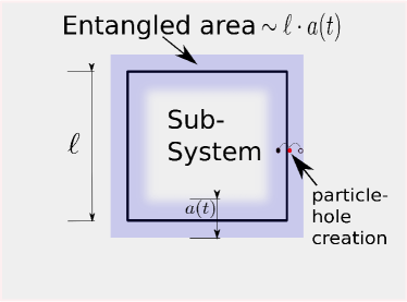
Figure 1: A quench in a two-dimensional system produces particle-hole pairs which propagate and create an entangled region which is proportional to the surface area $\sim\ell$ of the subsystem times the length $a(t)$ over which the pairs have spread. For a clean system, in particular, a linear growth in time, $S_{\textrm{ent}}\sim\ell\cdot vt$, with velocity $v$ is thus expected for $vt\ll\ell$.

According to this picture one expects that for times $vt\ll\ell$ the entanglement entropy grows as

$$S_{\textrm{ent}}\sim\ell^{d-1}\cdot t$$ (1)

while $S_{\textrm{ent}}\sim\ell^{d}$ at times $vt\gg\ell$. For quenches in free scalar field theories this picture is largely confirmed also in two and three dimensions Cotler et al. (2016).

II Fermions with potential disorder

In a classical system with potential disorder, fluctuations in the density will typically relax in a diffusive manner. To obtain the proper quantum mechanical picture for the spreading of excitations after the quench for fermions with disorder, the disorder averaged particle-hole propagator

$$\mathcal{D}(r,t)=\langle\langle\Psi^{\dagger}(r,t)\Psi(0,0)\rangle\langle\Psi(r,t)\Psi^{\dagger}(0,0)\rangle\rangle_{\textrm{dis}}$$ (2)

has to be calculated Vollhardt and P. (1980); Altland and Simons (2006). Apart from a classical contribution where hole and particle propagate in the same direction along the same path in configuration space (the diffuson contribution), there are now also processes where particle and hole traverse a path with opposite momenta (the cooperon contribution) which will lead to interference effects. Ultimately, such quantum corrections will result in a complete breakdown of diffusion—the fermions become Anderson localized Anderson (1958). It is well known that in one and two dimensions any amount of disorder is sufficient to completely localize all states Abrahams et al. (1979). For the entanglement entropy at sufficiently long times after the quench we therefore expect an area law $S_{\textrm{ent}}\sim\ell^{d-1}\xi_{\textrm{loc}}$ if $\xi_{\textrm{loc}}\ll\ell$ where $\xi_{\textrm{loc}}$ is the localization length, and $a(t\to\infty)\to\xi_{\textrm{loc}}$ see Fig. 1.

Here we want to investigate how a disordered system evolves towards this long-time limit. Contrary to the one-dimensional case where the localization length $\xi_{\textrm{loc}}$ is of the order of the mean free path $l_{m}$ and an initial ballistic spreading is immediately followed by saturation with no room for diffusion, the situation is much more complex in the two-dimensional case. Here the localization length for weak disorder is exponentially large as compared to $l_{m}$ so that we might expect three distinct time regimes for the entanglement entropy $S_{\textrm{ent}}(t)$. These regimes can be characterized using the elastic scattering time $\tau=l_{m}/v$: (i) $t\ll\tau$, initial ballistic increase, (ii) $\tau\ll t\ll\tau\exp(\varepsilon\tau/\hbar)$, intermediate regime, and (iii) $t\gg\tau\exp(\varepsilon\tau/\hbar)$, saturation (with $\varepsilon$ being the characteristic energy scale of the model). Understanding the intermediate regime is the main purpose of this section.

To be specific, we will consider a square $L\times L$ lattice with Hamiltonian

$$H=-\sum_{\langle i,j\rangle}J_{ij}c^{\dagger}_{i}c_{j}+\sum_{i}D_{i}c^{\dagger}_{i}c_{i},$$ (3)

where, $J_{ij}$ is the hopping amplitude between neighbouring sites (we set $J_{ij}=J$ in this section), $c_{i}$ and $c^{\dagger}_{i}$ are annihilation and creation operators of spinless fermions on site $i$, and $D_{i}$ is the on-site disorder potential. The potentials $D_{i}$ are drawn randomly from a box $[0,D)$. Motivated by recent experiments on cold atomic gases Schreiber et al. (2015) we choose as initial state a charge density wave (CDW) configuration where singly occupied and empty sites alternate in both spatial directions

$$|\Psi(0)\rangle=\prod_{i,j=1}^{L/2}c^{\dagger}_{2i,2j}c^{\dagger}_{2i-1,2j-1}|0\rangle\,.$$ (4)

Here $|0\rangle$ denotes the vacuum state. We want to emphasize that the results presented in the following do not qualitatively depend on the specific initial state chosen as long as the setup is not fine-tuned, e.g. in a way that the dynamics decouples and becomes one dimensional Zhao et al. (2017).

II.1 Entanglement entropy

To calculate the entanglement entropy we always choose a square with size $\frac{L}{2}\times\frac{L}{2}$ in the middle of the $L\times L$ lattice as the subsystem, i.e. $\ell\equiv L/2$ in the following. For a non-interacting system, the entanglement entropy of the subsystem can be obtained from its single-particle correlation matrix. If $\zeta_{i}$ are the eigenvalues of the correlation matrix of the subsystem then the entanglement entropy is given byChung and Peschel (2001); Peschel (2004); Peschel and Eisler (2009)

$$S_{\textrm{ent}}(t) \equiv -\text{tr}\{\rho_{\textrm{red}}\ln\rho_{\textrm{red}}\}$$

$$= -\sum_{i}\{\zeta_{i}\ln\zeta_{i}+(1-\zeta_{i})\ln(1-\zeta_{i})\}\,,$$

where $\rho_{\textrm{red}}$ is the reduced density matrix. Using exact diagonalization (ED) we are thus able to investigate the dynamics in relatively large two-dimensional lattices. We calculate disorder averages using $\sim 1000$ samples for $L\leq 30$ sites and at least $100$ samples for larger system sizes.

As a first check, we consider the unitary dynamics caused by the Hamiltonian (3) without disorder, see Fig. 2.

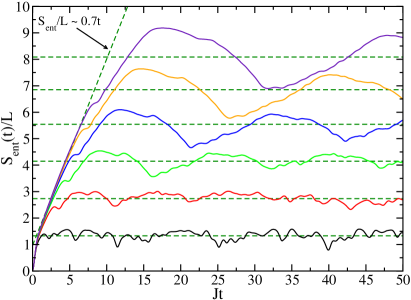
Figure 2: ED results for the entanglement entropy during unitary time evolution with the Hamiltonian (3) without disorder ($D_{i}\equiv 0$) starting from the CDW state (4). Shown are results for system sizes $10\times 10$, $\cdots$, $60\times 60$ (solid lines, from bottom to top). The dashed lines are fits of the initial linear increase and the long-time asymptotics, respectively.

After a quick initial increase at times $Jt\lesssim 1$ a linear scaling sets in which lasts up to $t_{0}=L/4v=L/8$. Consistent with the picture in Fig. 1 the whole interior at this point has built up some entanglement with the exterior and the increase of entanglement slows down. At long times, the entanglement entropy oscillates around $S_{\textrm{ent}}\approx 0.137L^{2}$ consistent with the expected volume law.

Next, we consider the case of strong potential disorder. Then an initial increase of the entanglement entropy is immediately followed by a saturation, see the inset of Fig. 3.

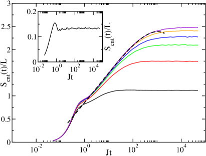
Figure 3: Inset: $S_{\textrm{ent}}(t)/L$ for $D=100$ and $L=40$. Main: Entanglement entropy for $D=10$ and system sizes $L=10,20,\cdots,60$ (from bottom to top). The dashed line is a fit in the intermediate time regime, see Eq. (9).

Most interesting is the case of small disorder where the localization length $\xi_{\textrm{loc}}$ is much larger than the mean free path $l_{m}$, see the main panel of Fig. 3. We can now indeed identify three distinct time regimes: For times $Jt\lesssim 1$ there is a fast initial increase. This is, however, now followed by an extended intermediate time regime. Note also that with increasing system size all data for $S_{\textrm{ent}}(t)/L$ fall onto a single curve showing that the system obeys an area instead of a volume law scaling. In the intermediate time regime—which for the chosen disorder extends from $1\lesssim Jt\lesssim 10^{3}$—the scaling is approximately logarithmic as in the one-dimensional many-body localized regime. In contrast to the latter case, however, no interactions are present and the logarithmic scaling is followed by a saturation at long times.

We show in the following that the logarithmic scaling can be understood as a weak localization effect. Calculating the disorder averaged particle-hole propagator (2) diagrammatically one finds

$$\mathcal{D}(q,\omega)\sim\frac{iD_{0}q^{2}}{\omega+iD_{0}q^{2}}$$ (6)

from summing up the ladder diagrams with non-crossing impurity lines, the diffuson contribution.Vollhardt and P. (1980); Altland and Simons (2006) The particle-hole propagator shows diffusion at this level of approximation with $D_{0}$ being the diffusion constant. Quantum corrections to this result come predominantly from maximally crossed diagrams, the cooperon contribution. These corrections involve integrations over the diffusion pole which leads to logarithmic corrections in two dimensions

$$\int\frac{q\,dq}{\omega+iD_{0}q^{2}}\stackrel{{\scriptstyle q\to 0}}{{\sim}}\ln\omega\,.$$ (7)

Here a cutoff for large $q$ implied. These corrections can be summed up as ladder-type diagrams leading to a logarithmic correction of the diffusion constant $D(\omega)$.Gor’kov et al. (1979) For the diffusive spreading in the weak-localization regime this means that the mean squared of the distance over which the particle-hole propagator has spread is given by $\langle r^{2}(t)\rangle=4D(t)t$ with a time-dependent diffusion constantNakhmedov et al. (1987); Sebbah et al. (1993)

$$D(t)=D_{0}[1-(A\hbar/\varepsilon\tau)\ln(t/\tau)]\,$$ (8)

with some dimensionless constant $A$. This perturbative result is expected to be valid for $\tau\ll t\ll\tau\exp(\varepsilon\tau/(A\hbar)$. For the growth of the entanglement entropy in this intermediate time regime this implies a scaling

$$S_{\textrm{ent}}(t)/L=\mbox{const}+at^{\alpha}\sqrt{1-b\ln(t/\tau)}$$ (9)

with $\alpha=1/2$. Fits using Eq. (9) do indeed show a good agreement with the numerical data although the best results are obtained using a smaller exponent $\alpha\approx 0.2$, see Fig. 3. If we expand the scaling function (9) around its inflection point we find, in particular, that $S_{\textrm{ent}}(t)/L\sim\mbox{const}+\ln(t/\tau)$. In the intermediate time regime the entanglement entropy does grow logarithmically.

II.2 CDW order parameter

We start the quench from the initial CDW state (4). This state has an order parameter

$$I=\frac{2}{L^{2}}\sum_{i,j}(-1)^{i+j}n_{i,j}=\frac{2}{L^{2}}\sum_{k_{x},k_{y}}c^{\dagger}_{k_{x},k_{y}}c_{k_{x}-\pi,k_{y}-\pi}$$ (10)

with $\langle\Psi(0)|I|\Psi(0)\rangle=1$ whose evolution we want to monitor as a function of time. The Fourier representation of the order parameter in (10) makes it clear that we are now looking at the time evolution of a single-particle Green’s function instead of the particle-hole propagator (2) relevant for the time evolution of the entanglement entropy. This means, in particular, that interference effects responsible for the weak localization phenomena discussed in the previous section are expected to be absent. The data shown in Fig. 4 are consistent with these expectations. A well-defined intermediate time regime does not exist. Note that in the numerics we calculate $\langle I\rangle(t)$ by taking the difference in occupation of two neighboring sites in the middle of the square lattice in order to reduce finite size effects.

Figure 4: Order parameter $\langle I\rangle(t)$. Left: Data for a $20\times 20$ lattice with box potential disorder $D=2,6,10$. Right: Box potential disorder $D=5$ and lattice sizes $L=10,30,60$. For clarity, running averages over intervals $Jt=2$ are shown. After an initial decrease on the scale $Jt\sim 1$, $\langle I\rangle(t)$ starts oscillating around the long-time mean.

For a clean two-dimensional square lattice it is easy to show that the order parameter in the thermodynamic limit will completely decay as $\langle I\rangle(t)=J^{2}_{0}(4Jt)\stackrel{{\scriptstyle t\to\infty}}{{\sim}}1/t$ where $J_{0}$ is the Bessel function of the first kindZhao et al. (2017). Fig. 4(a) shows that once the localization length becomes smaller than the system size, the order parameter does no longer decay completely but rather oscillates around a non-zero value after a quick initial decay on a time scale $t\sim 1/J$. While boundary effects remain present in the oscillations around the mean value, Fig. 4(b) shows that the long-time average starts to converge when increasing the system size.

II.3 Binary disorder and percolation threshold

Another interesting question for two-dimensional systems with potential disorder is the behavior near the percolation threshold. If we consider strong binary disorder $D_{i}\in\{-D/2,D/2\},\,D\gg 1$ then the system will be effectively cut into independent clusters of potential $+D$ or $-D$ with particles unable to hop from one to the other on time scales $t\ll D/J^{2}$.Andraschko et al. (2014); Enss et al. (2017); Sirker (2019) The site percolation threshold for a two-dimensional square lattice is $p_{c}\approx 0.592746...$. I.e., if we have a probability $0.4\lesssim p\lesssim 0.6$ for a site to have potential $+D/2$ ($1-p$ for a site to have potential $-D/2$) then both clusters will be non-percolating. Otherwise, one of the clusters will be percolating. In Fig. 5 results for the entanglement entropy for binary potential disorder $D=100$ and $p=0.5,\,0.2$, respectively, are shown.

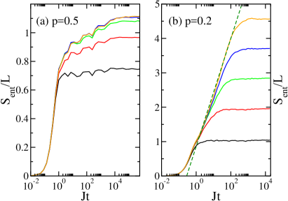
Figure 5: Binary potential disorder for $D=100$ and system sizes $L=10,20,\cdots,50$: (a) For $p=0.5$ the entanglement entropy shows area law scaling at long times. (b) Volume law scaling for $p=0.2$. The dashed line is a logarithmic fit of the intermediate time behavior.

For $p=0.5$ we find the expected area law scaling, i.e., results for $S_{\textrm{ent}}(t)/L$ do converge to a single curve for $L\to\infty$. More interesting is the percolating case $p=0.2$. Apart from the expected volume law scaling at long times, there is an interesting intermediate time regime which is quite different from the linear scaling due to the ballistic spreading of particle-hole pairs in the clean case shown in Fig. 1. Instead, the time dependence of $S_{\textrm{ent}}(t)$ seems to be consistent with a logarithmic increase. This is somewhat surprising given that the boundaries of a percolating cluster do perform a random walk and one might thus at least classically expect a power-law dependence. Quantum mechanically the problem is, of course, much more complicated. The randomly shaped percolating clusters will result in many different propagation paths which can interfere with each other. While this might qualitatively explain why the entanglement growth is much slower than in the clean case, we cannot offer a proper quantitative theory at this point. Importantly, there seems to be a second mechanism—apart from weak localization discussed previously—which can lead to a logarithmic or almost logarithmic scaling of the entanglement entropy at intermediate times. A logarithmic increase of $S_{\textrm{ent}}(t)$ is therefore not a ’smoking gun’ for many-body localization as it is considered to be in the one-dimensional case.

III Fermions with bond disorder

In contrast to potential disorder which always leads to localization in one and two dimensions, bond disordered systems can display in addition to a localized phase also infinite randomness fixed points (IRFP) where the system is critical.Eggarter and Riedinger (1978); Fisher (1994, 1992, 1995) In one dimension, eigenstates show a $S_{\textrm{ent}}\sim\ln\ell$ scaling at an IRFP. Since length is expected to scale as $\ell\sim|\ln t|^{\Psi}$ with dynamical critical exponent $\Psi$, the entanglement will therefore grow extremely slowly as $S_{\textrm{ent}}(t)\sim\ln\ln(t)$ at long times. Numerically, such log-log scaling of the entanglement entropy after a quench has been observed in the critical transverse Ising chainIglói et al. (2012) and the XX-chain Zhao et al. (2016). The situation is less settled in higher dimensions. For the critical two-dimensional transverse Ising model, an area law with multiplicative logarithmic corrections, $S_{\textrm{ent}}\sim\ell\ln(\ln\ell)$, has been suggested in Ref. Lin et al., 2007 while a second numerical study, Ref. Yu et al., 2008, has interpreted their results in terms of an additive logarithmic correction, $S_{\textrm{ent}}\sim a\ell+b\ln\ell$. In the latter study, it has been argued that the presence of an additive logarithmic correction is related to percolation. An additive logarithmic correction was later confirmed in large-scale numerical strong disorder renormalization group calculations and the dependence of the size of the logarithmic correction on the shape of the subsystem was studied Kovacs et al. (2012, 2012).

Here we want to examine the entanglement growth directly in the microscopic two-dimensional free fermion model (3) with bond disorder. In order to study the connection to percolation, we concentrate on the case of binary bond disorder. If we have bonds drawn from $J_{ij}\in\{0,1\}$ then the classical percolation threshold is $p_{c}=0.5$. For this type of bond disorder we might thus expect that the entanglement entropy follows an area law if the probability for a bond being present ($J_{ij}=1$) is given by $p<p_{c}$ while a volume law should hold for $p>p_{c}$. To study the generic dynamics near the percolation threshold we present in Fig. 6 data for binary disorder $J_{ij}\in\{0.05,0.95\}$ on a square $L\times L$ lattice with a subsystem size $\ell=L/2$.

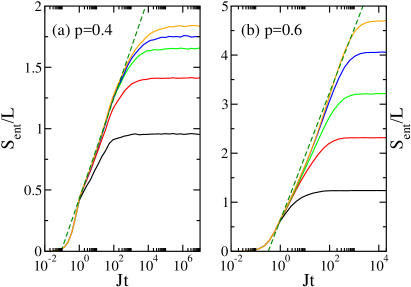
Figure 6: Binary bond disorder $J_{ij}\in\{0.05,0.95\}$: (a) for a probability $p=0.4$ to have a strong bond the long-time scaling seems to approximately follow and area law, while (b) for $p=0.6$ the scaling appears close to a volume law. The dashed lines are logarithmic fits at intermediate times.

For both probabilities $p$ to have a strong bond shown in Fig. 6, the entanglement entropy per length $L$ increases approximately logarithmically at intermediate times before starting to saturate. While the scaling at long times in Fig. 6(a) for $p=0.4$ appears to be close to an area law, the curves for the largest system sizes studied do not fall on top of each other and show a slow convergence towards the saturation value. To investigate this behavior further we show in Fig. 7(a) the saturation values at long times for the case $p=0.4$ as a function of length $L$.

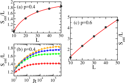
Figure 7: Binary bond disorder $J_{ij}\in\{0.05,0.95\}$: (a) Saturation values at long times versus $L$ (circles) and fit $S_{\textrm{ent}}/L=a+b(\ln L)/L$ (line). (b) Long-time behavior and fit $S_{\textrm{ent}}/L=a^{\prime}+b^{\prime}\ln(\ln t)/(\ln t)^{\Psi}$ with $\Psi\sim 0.4$. (c) Saturation values and fit $S_{\textrm{ent}}/L=\tilde{a}L+\tilde{b}L\ln L$.

The entanglement per area is well fitted by $S_{\textrm{ent}}/L=a+b(\ln L)/L$ supporting an area law with an additive logarithmic corrections as suggested in Ref. Yu et al., 2008. Furthermore, the expected scaling $L(t)\sim(\ln t)^{\Psi}$ at an IRFP yields a very good fit of the long-time behavior, see Fig. 7(b). On the other side of the percolation transition we find saturation values of the entanglement entropy which are consistent with a volume law scaling with an additive logarithmic correction, see Fig. 7(c). Using again the expected scaling relation between length and time leads to a logarithmic scaling consistent with the data shown in Fig. 6(b). Overall, our data are consistent with additive logarithmic corrections to the area and volume laws on either side of the percolation transition and IRFP behavior, $L(t)\sim(\ln t)^{\Psi}$, at long times.

IV Summary and conclusions

Quenching two-dimensional free fermion systems with potential and binary disorder, we have identified several cases where the entanglement entropy $S_{\textrm{ent}}(t)$ shows a logarithmic growth as a function of time $t$ as well as logarithmic corrections to area and volume laws.

The behavior of $S_{\textrm{ent}}(t)$ for potential disorder can be understood in a picture of particle-hole pairs created by quenching the system. As is well known, the particle-hole propagator consists of a classical diffuson and a quantum correction, the cooperon contribution. In the intermediate time regime $\tau\ll t\ll\tau\exp(\varepsilon\tau/\hbar)$, where $\tau$ is the elastic scattering time, the interference effects due to the latter contribution lead to weak localization. We have shown that weak localization results in a logarithmic growth of the entanglement entropy per area, $S_{\textrm{ent}}(t)/L\sim\mbox{const}+\ln(t/\tau)$, before Anderson localization and thus a saturation of $S_{\textrm{ent}}(t)/L$ ultimately sets in at times $t\gg\tau\exp(\varepsilon\tau/\hbar)$. We demonstrated, furthermore, that the weak localization regime does not materialize in a local order parameter: here the relevant quantity is the single particle Green’s function which—in contrast to the particle-hole propagator—does not show interference effects. For experiments on cold atomic gases this means that a monitoring of local order parameters as in Ref. Schreiber et al., 2015; Bordia et al., 2017 would not be sufficient to observe weak localization. Instead, the recently demonstrated direct measurements of number and configurational entropiesLukin et al. (2019) offer an avenue to explore this regime if generalized and applied to the two-dimensional case.

For the case of bond disorder, we have concentrated on a binary distribution where strong bonds occur with probability $p$ and weak bonds with probability $1-p$. For strong binary bond disorder, we have found qualitatively different behavior for the entanglement entropy after quenching from a product state based on whether or not $p$ is smaller or larger than the classical percolation threshold $p_{c}=0.5$. While $S_{\textrm{ent}}(t)$ at long times is approximately showing an area law scaling for $p<p_{c}$ we find approximately a volume law for $p>p_{c}$. Interestingly, there are additive logarithmic corrections present in both cases consistent with IRFP behavior. For the case $p<p_{c}$ the logarithmic corrections lead, in particular, to a very slow increase of the entanglement entropy at long times, $S_{\textrm{ent}}(t)/L\sim\ln\ln t/(\ln t)^{\Psi}$, with dynamical critical exponent $\Psi$.

In conclusion, we have demonstrated that the entanglement entropy of two-dimensional disordered fermion systems shows a very rich and interesting behavior as a function of time after a global quench. We have explained the logarithmic growth in the potential disorder case by weak localization physics and the logarithmic corrections to area and volume laws as well as the long-time scaling in the bond disordered case by IRFP physics. While our work does not address the interacting case and the question whether or not many-body localized phases exist in two-dimensional quantum systems, the results obtained here might be helpful to develop criteria to distinguish possible MBL phases from Anderson physics and IRFP behavior.