Nektar++: enhancing the capability and application of high-fidelity spectral/$hp$ element methods

Abstract

Nektar++ is an open-source framework that provides a flexible, high-performance and scalable platform for the development of solvers for partial differential equations using the high-order spectral/$hp$ element method. In particular, Nektar++ aims to overcome the complex implementation challenges that are often associated with high-order methods, thereby allowing them to be more readily used in a wide range of application areas. In this paper, we present the algorithmic, implementation and application developments associated with our Nektar++ version 5.0 release. We describe some of the key software and performance developments, including our strategies on parallel I/O, on in situ processing, the use of collective operations for exploiting current and emerging hardware, and interfaces to enable multi-solver coupling. Furthermore, we provide details on a newly developed Python interface that enables a more rapid introduction for new users unfamiliar with spectral/$hp$ element methods, C++ and/or Nektar++. This release also incorporates a number of numerical method developments – in particular: the method of moving frames (MMF), which provides an additional approach for the simulation of equations on embedded curvilinear manifolds and domains; a means of handling spatially variable polynomial order; and a novel technique for quasi-3D simulations (which combine a 2D spectral element and 1D Fourier spectral method) to permit spatially-varying perturbations to the geometry in the homogeneous direction. Finally, we demonstrate the new application-level features provided in this release, namely: a facility for generating high-order curvilinear meshes called NekMesh; a novel new AcousticSolver for aeroacoustic problems; our development of a ‘thick’ strip model for the modelling of fluid-structure interaction (FSI) problems in the context of vortex-induced vibrations (VIV). We conclude by commenting on some lessons learned and by discussing some directions for future code development and expansion.

PROGRAM SUMMARY

Manuscript Title: Nektar++: enhancing the capability and application of high-fidelity spectral/$hp$ element methods
Authors: D. Moxey, C. D. Cantwell, Y. Bao, A. Cassinelli, G. Castiglioni, S. Chun, E. Juda, E. Kazemi, K. Lackhove, J. Marcon, G. Mengaldo, D. Serson, M. Turner, H. Xu, J. Peiró, R. M. Kirby, S. J. Sherwin
Program Title: Nektar++
Journal Reference:
Catalogue identifier:
Licensing provisions: MIT
Programming language: C++
Computer: Any PC workstation or cluster
Operating system: Linux/UNIX, macOS, Microsoft Windows
RAM: 512 MB+
Number of processors used: 1-1024+
Supplementary material:
Keywords: spectral/$hp$ element method, computational fluid dynamics
Classification: 12 Gases and Fluids
External routines/libraries: Boost, METIS, FFTW, MPI, Scotch, PETSc, TinyXML, HDF5, OpenCASCADE, CWIPI
Nature of problem: The Nektar++ framework is designed to enable the discretisation and solution of time-independent or time-dependent partial differential equations.
Solution method: spectral/$hp$ element method
Reasons for the new version:*
Summary of revisions:*
Restrictions:
Unusual features:
Additional comments:
Running time: The tests provided take a few minutes to run. Runtime in general depends on mesh size and total integration time.

1 Introduction

High-order finite element methods are becoming increasingly popular in both academia and industry, as scientists and technological innovators strive to increase the fidelity and accuracy of their simulations whilst retaining computational efficiency. The spectral/$hp$ element method in particular, which combines the geometric flexibility of classical low-order finite element methods with the attractive convergence properties of spectral discretisations, can yield a number of advantages in this regard. From a numerical analysis perspective, their diffusion and dispersion characteristics mean that they are ideally suited to applications such as fluid dynamics, where flow structures must be convected across long time- and length-scales without suffering from artificial dissipation [1, 2, 3, 4, 5] High-order methods are also less computationally costly than traditional low-order numerical schemes for a given number of degrees of freedom, owing to their ability to exploit a more locally compact and dense elemental operators when compared to sparse low-order discretisations [6, 7, 8]. In addition, high-order methods in various formulations can be seen to encapsulate other existing methods, such as finite volume, finite difference (e.g. summation-by-parts finite difference [9]), finite element, and flux reconstruction approaches [10, 11]. All of these features make the spectral/$hp$ element method an extremely attractive tool to practitioners.

As the name suggests, the spectral/$hp$ element method relies on the tesselation of a computational domain into a collection of elements of arbitrary size that form a mesh, where each element is equipped with a polynomial expansion of arbitrary and potentially spatially-variable order [12]. Within this definition, we include continuous Galerkin (CG) and discontinuous Galerkin (DG) methods, along with their variants. High-order methods have been historically seen as complex to implement, and their adoption has been consequently limited to academic groups and numerical analysts. This mantra is rapidly being removed thanks to the development of open-source numerical libraries that facilitate the implementation of new high-fidelity solvers for the solution of problems arising across a broad spectrum of research areas in engineering, biomedicine, numerical weather and climate prediction, and economics. An additional challenge in the use of high-order methods, particularly for problems involving complex geometries, is the generation of a curvilinear mesh that conforms to the underlying curves and surfaces. However, advances in curvilinear mesh generation (such as [13]), combined with open-source efforts to increase their prevalence, mean that simulations across extremely complex geometries are now possible.

Nektar++ is a project initiated in 2005 (the first commit to an online repository was made on 4^th May 2006), with the aim of facilitating the development of high-fidelity computationally-efficient, and scalable spectral element solvers, thereby helping close the gap between application-domain experts (or users), and numerical-method experts (or developers). Along with Nektar++, other packages that implement such high-order methods have been developed in the past several years. Nek5000, developed at Argonne National Laboratory, implements CG discretizations mainly for solving incompressible and low-Mach number flow problems on hexahedral meshes using the classical spectral element method of collocated Lagrange interpolants [14]. Semtex [15, 16] is a fluid dynamics code that also uses the classical spectral element method in two dimensions, with the use of a 1D pseudospectral Fourier expansion for three dimensional problems that incorporate a homogeneous component of geometry. Nektar++ also supports this joint discretisation in Cartesian coordinates; however Semtex also includes support for cylindrical coordinate systems, where the Fourier modes are used in the azimuthal direction, which broadens the range of geometries that can be considered in this setting. deal.II [17] is a more generic finite element framework, which likewise restricts its element choices to quadrilaterals and hexahedra, but permits the solution of a wide array of problems, alongside the use of adaptive mesh refinement. Flexi [18] and its spinoff Fluxo [19], developed at the University of Stuttgart and at the University of Cologne, implement discontinuous Galerkin methods for flow problems on hexahedral meshes. GNuME, and its NUMO and NUMA components developed at the Naval Postgraduate School, implement both continuous and discontinuous Galerkin methods mainly for weather and climate prediction purposes [20, 21]. PyFR [22], developed at Imperial College London, implements the flux reconstruction approach [23] which shares various numerical properties with DG in particular [10, 24]. DUNE implements a DG formulation, among a wide variety of other numerical methods such as finite difference and finite volume methods [25].

Nektar++ is a continuation of an earlier code Nektar, itself developed at Brown University originally using the C programming language, with some parts extended to use C++. Nektar++ is instead written using the C++ language, and greatly exploits its object-oriented capabilities. The aim of Nektar++ is to encapsulate many of the high-order discretisation strategies mentioned previously, in a readily accessible framework. The current release includes both CG and DG methods and, arguably, its distinguishing feature is its inherent support for complex geometries through various unstructured high-order element types; namely hexahedra, tetrahedra, prisms and pyramids for three-dimensional problems, and quadrilaterals and triangles for two-dimensional problems. Both CG and DG can be used on meshes that contain different element shapes (also referred to as hybrid meshes), and allow for curvilinear element boundaries in proximity of curved geometrical shapes. Along with these spatial discretizations, Nektar++ supports so-called quasi-3D simulations in a manner similar to Semtex, where a geometrically complex 2D spectral element mesh is combined with a classical 1D Fourier expansion in a third, geometrically homogeneous, direction. This mixed formulation can significantly enhance computational efficiency for problems of the appropriate geometry [15] and Nektar++ supports a number of different parallelisation strategies for this approach [26]. The time discretization is achieved using a general linear method formulation for the encapsulation of implicit, explicit and mixed implicit-explicit timestepping schemes [27]. While the main purpose of the library is to create an environment under which users can develop novel solvers for the applications of their interest, Nektar++ already includes fully-fledged solvers for the solution of several common systems, including fluid flows governed either by the incompressible or compressible Navier-Stokes and Euler equations; advection-diffusion-reaction problems, including on a manifold, with specific applications to cardiac electrophysiology [28]. One of the main shortcomings of the spectral/$hp$ element method is related to a perceived lack of robustness, arising from low dissipative properties, which can be a significant challenge for industrial applications. Nektar++ implements several techniques to address this problem, namely efficient dealiasing techniques [29, 30] and spectral vanishing viscosity [31], that have proved invaluable for particularly challenging applications [32].

The scope of this review is to highlight the substantial number of new developments in Nektar++ since the last publication related to the software, released in 2015 and coinciding with the version 4 release of Nektar++ [33]. Since this release, over 7,000 commits have been added to the main code for the version 5 documented here, with a key focus on expanding the capability of the code to provide efficient high-fidelity simulations for challenging problems in various scientific and engineering fields. To this end, the paper is organized as follows. After a brief review of the formulation in Section 2, in Section 3 we present our software and performance developments. This includes our strategies on parallel I/O; in situ processing; the use of collective linear algebra operations for exploiting current and emerging hardware; and interfaces for multi-solver coupling to enable multi-physics simulations using Nektar++. Furthermore, we provide details on our new Python interfaces that enable more rapid on-boarding of new users unfamiliar with either spectral/$hp$ element methods, C++ or Nektar++. In Section 4, we then present recent numerical method developments – in particular, the method of moving frames (MMF); recently added support for spatially-variable polynomial order for $p$-adaptive simulations; and new ways of incorporating global mappings to enable spatially variable quasi-3D approaches. In Section 5, we then demonstrate some of the new features provided in our new release, namely: our new facility for generating high-order (curvilinear) meshes called NekMesh; a new AcousticSolver for aeroacoustic problems; and our development of a ‘thick’ strip model for enabling the solution of fluid-structure interaction (FSI) problems in the context of vortex-induced vibrations (VIV). We conclude in Section 7 by commenting on some lessons learned and by discussing some directions for future code development and expansion.

Contributors

Nektar++ has been developed across more than a decade, and we would like to explicitly acknowledge the many people who have made contributions to the specific application codes distributed with the libraries. In addition to the coauthors of the previous publication [33] we would like to explicitly thank the following for their contributions:

• Dr. Rheeda Ali (Department of Biomedical Engineering, Johns Hopkins University, USA) and Dr. Caroline Roney (Biomedical Engineering Department, King’s College London, UK) for their work on the cardiac electrophysiology solver;

• Dr. Michael Barbour and Dr. Kurt Sansom (Department of Mechnical Engineering, University of Washington, USA) for developments related to biological flows;

• Mr. Filipe Buscariolo (Department of Aeronautics, Imperial College London, UK) for contributions to the incompressible Navier-Stokes solver;

• Dr. Jeremy Cohen (Department of Aeronautics, Imperial College London, UK) for work relating to cloud deployment and the Nekkloud interface;

• Mr. Ryan Denny (Department of Aeronautics, Imperial College London, UK) for enhancements in the 1D arterial pulse wave model;

• Mr. Jan Eichstädt (Department of Aeronautics, Imperial College London, UK) for initial investigations towards using many-core and GPU platforms;

• Dr. Stanisław Gepner (Faculty of Power and Aeronautical Engineering, Warsaw University of Technology, Poland) for enhancements in the Navier-Stokes linear stability solver;

• Mr. Dav de St. Germain (SCI Institute, University of Utah, USA) for enhancements of timestepping schemes;

• Mr. Ashok Jallepalli (SCI Institute, University of Utah, USA) for initial efforts on the integration of SIAC filters into post-processing routines;

• Prof. Dr. Johannes Janicka (Department of Energy and Power Plant Technology), Technische Universität Darmstadt, Germany), for support and development of the acoustic solver and solver coupling;

• Mr. Edward Laughton (College of Engineering, Mathematics and Physical Sciences, University of Exeter, UK) for testing enhancements and initial efforts on non-conformal grids;

• Dr. Rodrigo Moura (Divisão de Engenharia Aeronáutica, Instituto Tecnológico de Aeronáutica, Brasil) for numerical developments related to spectral vanishing viscosity stabilisation;

• Dr. Rupert Nash and Dr. Michael Bareford (EPCC, University of Edinburgh, UK) for their work on parallel I/O; and

• Mr. Zhenguo Yan and Mr. Yu Pan (Department of Aeronautics, Imperial College London, UK) for development of the compressible flow solver;

2 Methods

In this first section, we outline the mathematical framework that underpins Nektar++, as originally presented in [33, 34]. Nektar++ supports a variety of spatial discretisation choices, primarily based around the continuous and discontinuous Galerkin methods (CG and DG). However, in the majority of cases CG and DG use the same generic numerical infrastructure. Here we therefore present a brief overview and refer the reader to [12] for further details, which contains a comprehensive description of the method and its corresponding implementation choices. In the text below we also highlight appropriate chapters and sections from [12] for the material being discussed.

The broad goal of Nektar++ is to provide a framework for the numerical solution of partial differential equations (PDEs) of the form $\mathcal{L}u=0$ on a domain $\Omega$, which may be geometrically complex, for some solution $u$. Practically, in order to carry out a spatial discretisation of the PDE problem, $\Omega$ needs to be partitioned into a finite number of $d$-dimensional non-overlapping elements $\Omega_{e}$, where in Nektar++ we support $1\leq d\leq 3$, such that the collection of all elements recovers the original region ($\Omega=\bigcup\Omega_{e}$) and for $e_{1}\neq e_{2}$, $\Omega_{e_{1}}\cap\Omega_{e_{2}}=\partial\Omega_{e_{1}e_{2}}$ is an empty set or an interface of dimension $\bar{d}<d$. The domain may be embedded in a space of equal or higher dimension, $\hat{d}\geq d$, as described in [28]. One of the distinguishing features of Nektar++ is that it supports a wide variety of elemental shapes: namely segments in one dimension [12, §2]; triangles and quadrilaterals in two dimensions, and; tetrahedra, pyramids, prisms and hexahedra in three dimensions [12, §3 and §4]. This makes it broadly suitable for the solution of problems in complex domains, in which hybrid meshes of multiple elements are generally required.

Nektar++ supports the solution of PDE systems that are either steady-state or time-dependent; in the case of time-dependent cases, there is subsequently a choice to use either explicit, implicit or implicit-explicit timestepping. From an implementation and formulation perspective, steady-state and implicit-type problems typically require the efficient solution of a system of linear equations, whereas explicit-type problems rely on the evaluation of the spatially discretised mathematical operators. In the following sections, we briefly outline the support in Nektar++ for these regimes.

2.1 Implicit-type methods

In this approach we follow the standard finite element derivation as described in [12, §2.2], so that before establishing the spatial discretisation, the abstract operator form $\mathcal{L}u=0$ is formulated in the weak sense alongside appropriate test and trial spaces $\mathcal{V}$ and $\mathcal{U}$. In general, we require at least a first-order derivative and select, for example, $\mathcal{V}=H^{1}_{0}(\Omega):=\{v\in H^{1}(\Omega)\ |\ v(\partial\Omega)=0\}$, where

$$H^{1}(\Omega):=\{v\in L^{2}(\Omega)\,|\,D^{\alpha}u\in L^{2}(\Omega)\,\forall\,|\alpha|\leq 1\}.$$

Following the Galerkin approach, we select $\mathcal{U}=\mathcal{V}$. We note that where problems involve Dirichlet boundary conditions on a boundary $\partial\Omega_{D}\subset\Omega$ of the form $u|_{\partial\Omega_{D}}(\bm{x})=g_{D}(\bm{x})$, we typically enforce this by lifting $g_{D}$ as described in [12, §2.2.3 and §4.2.4]. For illustrative purposes, we assume that $\mathcal{L}$ is linear and its corresponding weak form can be expressed as: find $u\in\mathcal{U}$ such that

$$a(u,v)=\ell(v)\quad\forall v\in\mathcal{U},$$ (1)

where $a(\cdot,\cdot)$ is a bilinear form and $\ell(\cdot)$ is a linear form.

To numerically solve the problem given in Equation 1 with the spatial partition of $\Omega$, we consider solutions in an appropriate finite-dimensional subspace $\mathcal{U}_{N}\subset\mathcal{U}$. In a high-order setting, these spaces correspond to the choice of spatial discretisation on the mesh. For example, in the discontinuous setting we select

$$\mathcal{U}_{N}=\{u\in L^{2}(\Omega)\ |\ u|_{\Omega_{e}}\in\mathcal{P}_{P}(\Omega_{e})\},$$

where $\mathcal{P}_{P}(\Omega_{e})$ represents the space of polynomials on $\Omega_{e}$ up to total degree $P$, so that functions are permitted to be discontinuous across elemental boundaries. In the continuous setting, we select the same space intersected with $C^{0}(\Omega)$, so that expansions are continuous across elemental boundaries. The solution to the weak form in Equation (1) can then be cast as: find $u^{\delta}\in\mathcal{U}_{N}$ such that

$$a(u^{\delta},v^{\delta})=\ell(v^{\delta})\quad\forall v^{\delta}\in\mathcal{U}_{N}$$ (2)

Assuming that the solution can be represented as $u^{\delta}(\bm{x})=\sum_{n}\hat{u}_{n}\Phi_{n}(\bm{x})$, a weighted sum of $N$ trial functions $\Phi_{n}(\bm{x})\in\mathcal{U}_{N}$ defined on $\Omega$ [12, §2.1], the problem then becomes that of finding the coefficients $\hat{u}_{n}$, which in the Galerkin approach translates into the solution of a system of linear equations.

Figure 1: Coordinate systems and mappings between collapsed coordinates $\bm{\eta}$, reference coordinates $\bm{\xi}$ and Cartesian coordinates $\bm{x}$ for a high-order triangular element $\Omega_{e}$.

To establish the global basis $\bm{\Phi}(\Omega)=\{\Phi_{1}(\bm{x}),\dots,\Phi_{N}(\bm{x})\}$, we first consider the contributions from each element in the domain. To simplify the definition of basis functions on each element, we follow the standard approach described in [12, §2.3.1.2 and §4.1.3] where $\Omega_{e}$ is mapped from a standard reference space $\mathcal{E}\subset[-1,1]^{d}$ by a parametric mapping $\bm{\chi}_{e}:\mathcal{E}\to\Omega_{e}$, so that $\bm{x}=\bm{\chi}_{e}(\bm{\xi})$. Here, $\mathcal{E}$ is one of the supported region shapes in Table 1 and $\bm{\xi}$ are $d$-dimensional coordinates representing positions in a reference element, distinguishing them from $\bm{x}$ which are $\hat{d}$-dimensional coordinates in the Cartesian coordinate space. On triangular, tetrahedral, prismatic and pyramid elements, one or more of the coordinate directions of a quadrilateral or hexahedral region are collapsed to form the appropriate reference shape, creating one or more singular vertices within these regions [35, 36]. Operations, such as calculating derivatives, map the tensor-product coordinate system to these shapes through Duffy transformations [37] — for example, $\bm{\omega}_{\mathcal{T}}:\mathcal{T}\rightarrow\mathcal{Q}$ maps the triangular region $\mathcal{T}$ to the quadrilateral region $\mathcal{Q}$ — to allow these methods to be well-defined. The relationship between these coordinates is depicted in Figure 1. Note that the singularity in the inverse mapping $\bm{\omega}^{-1}_{\mathcal{T}}$ does not affect convergence order and can be mitigated in practice by adopting an alternative choice of quadrature, such as Gauss-Radau points, in order to omit the collapsed vertices [12, §4.1.1].

The mapping $\bm{\chi}_{e}$ need not necessarily exhibit a constant Jacobian, so that the resulting element is deformed as shown in Figure 1. Nektar++ represents the curvature of these elements by taking a sub- or iso-parametric mapping for $\bm{\chi}_{e}$, so that the curvature is defined using at least a subset of the basis functions used to represent the solution field [12, §4.3.5]. The ability to use such elements in high-order simulations is critical in the simulation of complex geometries, as without curvilinear elements, one could not accurately represent the underlying curves and surfaces of the geometry, as demonstrated in [38]. The generation of meshes involving curved elements is, however, a challenging problem. Our efforts to generate such meshes, as well as to adapt linear meshes for high-order simulations, are implemented in the NekMesh generator tool described in Section 5.1, as well as a number of recent publications (e.g. [13, 39]).

Name	Class	Domain definition
Segment	StdSeg	$\mathcal{S}=\{\xi_{1}\in[-1,1]\}$
Quadrilateral	StdQuad	$\mathcal{Q}=\{\bm{\xi}\in[-1,1]^{2}\}$
Triangle	StdTri	$\mathcal{T}=\{\bm{\xi}\in[-1,1]^{2}\,|\,\xi_{1}+\xi_{2}\leq 0\}$
Hexahedron	StdHex	$\mathcal{H}=\{\bm{\xi}\in[-1,1]^{3}\}$
Prism	StdPrism	$\mathcal{R}=\{\bm{\xi}\in[-1,1]^{3}\,|\,\xi_{1}\leq 1,\xi_{2}+\xi_{3}\leq 0\}$
Pyramid	StdPyr	$\mathcal{P}=\{\bm{\xi}\in[-1,1]^{3}\,|\,\xi_{1}+\xi_{3}\leq 0,\xi_{2}+\xi_{3}\leq 0\}$
Tetrahedron	StdTet	$\mathcal{A}=\{\bm{\xi}\in[-1,1]^{3}\,|\,\xi_{1}+\xi_{2}+\xi_{3}\leq-1\}$

Table 1: List of supported elemental reference regions.

With the mapping $\bm{\chi}_{e}$ and the transformation $\bm{\omega}_{\mathcal{T}}$ the discrete approximation $u^{\delta}$ to the solution $u$ on a single element $\Omega_{e}$ can then be expressed as

$$u^{\delta}(\bm{x})=\sum_{n}\hat{u}_{n}\phi_{n}\left(\left[\bm{\chi}_{e}\right]^{-1}(\bm{x})\right)$$

where $\phi_{n}$ form a basis of $\mathcal{P}_{P}(\mathcal{E})$; i.e. a local polynomial basis need only be constructed on each reference element. A one-dimensional order-$P$ basis is a set of polynomials $\phi_{p}(\bm{\xi})$, $0\leq p\leq P$, defined on the reference segment, $\mathcal{S}$. The choice of basis is usually made based on its mathematical or numerical properties and may be modal or nodal in nature [12, §2.3]. For two- and three-dimensional regions, a tensorial basis may be employed, where the polynomial space is constructed as the tensor-product of one-dimensional bases on segments, quadrilaterals or hexahedral regions. In spectral/$hp$ element methods, a common choice is to use a modified hierarchical Legendre basis (a ‘bubble’-like polynomial basis sometimes referred to as the ‘modal basis’), given in [12, §3.2.3] as a function of one variable by

$$\phi_{p}(\xi)=\left\{\begin{array}[]{ll}\frac{1-\xi}{2}&p=0,\\ \left(\frac{1-\xi}{2}\right)\left(\frac{1+\xi}{2}\right)P^{1,1}_{p-1}(\xi)&0<p<P,\\ \frac{1+\xi}{2}&p=P,\end{array}\right.$$

which supports boundary-interior decomposition and therefore improves numerical efficiency when solving the globally assembled system. Equivalently, $\phi_{p}(\xi)$ could also be defined by the Lagrange polynomials through the Gauss-Lobatto-Legendre quadrature points which would lead to a traditional spectral element method [12, §2.3.4]. In higher dimensions, a tensor product of either basis can be used on quadrilateral and hexahedral elements respectively. On the other hand, the use of a collapsed coordinate system also permits the use of a tensor product modal basis for the triangle, tetrahedron, prism and pyramid, which when combined with tensor contraction techniques can yield performance improvements. This aspect is considered further in Section 3.3 and [40, 41].

Elemental contributions to the solution may be assembled to form a global solution through an assembly operator [12, §2.3.1 and §4.2.1]. In a continuous Galerkin setting, the assembly operator sums contributions from neighbouring elements to enforce the $C^{0}$-continuity requirement. In a discontinuous Galerkin formulation, such mappings transfer flux values from the element interfaces into the global solution vector. For elliptic operators, Nektar++ has a wide range of implementation choices available to improve computational performance. A common choice is the use of a (possibly multi-level) static condensation of the assembled system [12, §4.1.6 and §4.2.3], where a global system is formed only on elemental boundary degrees of freedom. This is supported both for the classical continuous framework, as well as in the DG method. In the latter, this gives rise to the hybridizable discontinuous Galerkin (HDG) approach [42], in which a global system is solved on the trace or skeleton of the overall mesh.

2.2 Explicit-type methods

Nektar++ has extensive support for the solution of problems in a time-explicit manner, which requires the evaluation of discretised spatial operators alongside projection into the appropriate space. As the construction of the implicit operators requires these same operator evaluations, most of the formulation previously discussed directly translates to this approach. We do note however that there is a particular focus on the discontinous Galerkin method as shown in [12, §6.2] for multi-dimensional hyperbolic systems of the form

$$\diff{{\bm{u}}}{t}+\nabla\cdot\bm{F}(\bm{u})=\bm{G}(\bm{u}).$$

This includes the acoustic perturbation equations that we discuss in Section 5.2 and the compressible Navier-Stokes system used for aerodynamics simulations in Section 5.4. In this setting, on a single element, and further assuming $\bm{G}$ is zero for simplicity of presentation as in [12, §6.2.2], we multiply the above equation by an appropriate test function $v\in\mathcal{U}$ and integrate by parts to obtain

$$\int_{\Omega_{e}}\diff{{\bm{u}}}{t}v\,\mathrm{d}\bm{x}+\int_{\partial\Omega_{e}}v\tilde{\bm{f}}^{e}(\bm{u}^{-},\bm{u}^{+})\cdot\bm{n}\,\mathrm{d}s-\int_{\Omega_{e}}\nabla v\cdot\bm{F}(\bm{u})\,\mathrm{d}\bm{x}=0.$$

In the above, $\tilde{\bm{f}}^{e}(\bm{u}^{-},\bm{u}^{+})$ denotes a numerically calculated boundary flux, depending on the element-interior velocity $\bm{u}^{-}$ and its neighbour’s velocity $\bm{u}^{+}$. The choice of such a flux is solver-specific and may invovle an upwinding approach or use of an appropriate Riemann solver. Where second-order diffusive terms are required, Nektar++ supports the use of a local discontinous Galerkin (LDG) approach to minimize the stencil required for communication (see [43] and [12, §7.5.2]). From a solver perspective, the implementation of the above is fairly generic, requiring only the evaluation of the flux term $\tilde{\bm{f}}$, conservation law $\bm{F}(\bm{u})$ and right-hand side source terms $\bm{G}(\bm{u})$.

2.3 Recap of Nektar++ implementation

In this section, we briefly outline the implementation of these methods inside Nektar++. Further details on the overall design of Nektar++, as well as examples of how to use it, can be found in the previous publication [33].

The core of Nektar++ comprises six libraries which are designed to emulate the general mathematical formulation expressed above. They describe the problem in a hierarchical manner, by working from elemental basis functions and shapes through to a C++ representation of a high-order field and complete systems of partial differential equations on a complex computational domain. Depending on the specific application, this then allows developers to choose an appropriate level for their needs, balancing ease of use at the highest level with fine-level implementation details at the lowest. A summary of each library’s purpose is the following:

• LibUtilites: elemental basis functions $\psi_{p}$, quadrature point distributions $\xi_{i}$ and basic building blocks such as I/O handling;

• StdRegions: reference regions $\mathcal{E}$ along with the definition of key finite element operations across them, such as integration, differentiation and transformations;

• SpatialDomains: the geometric mappings $\chi_{e}$ and factors $\frac{\partial\chi}{\partial\xi}$, as well as Jacobians of the mappings and the construction of the topology of the mesh from the input geometry;

• LocalRegions: physical regions in the domain, composing a reference region $\mathcal{E}$ with a map $\chi_{e}$, extensions of core operations onto these regions;

• MultiRegions: list of physical regions comprising $\Omega$, global assembly maps which may optionally enforce continuity, construction and solution of global linear systems, extension of local core operations to domain-level operations; and

• SolverUtils: building blocks for developing complete solvers.

In version 5.0, four additional libraries have been included. Each of these can be seen as a non-core, in the sense that they provide additional functionality to the core libraries above:

• Collections: encapsulates the implementation of key kernels (such as inner products and transforms) with an emphasis on evaluating operators collectively for similar elements;

• GlobalMapping: implements a mapping technique that allows quasi-3D simulations (i.e. those using a hybrid 2D spectral element/1D Fourier spectral discretisation) to define spatially-inhomogeneous deformations;

• NekMeshUtils: contains interfaces for CAD engines and key mesh generation routines, to be used by the NekMesh mesh generator; and

• FieldUtils: defines various post-processing modules that can be used both by the post-processing utility FieldConvert, as well as solvers for in-situ processing.

We describe the purpose of these libraries in greater detail in Sections 3.3, 4.3, 5.1 and 3.2 respectively.

3 Software and Performance Developments

This section reviews the software and performance developments added to Nektar++ since our last major release. We note that a significant change from previous releases is the use of C++11-specific language features throughout the framework. A brief summary of our changes in this area include:

• transitioning from various data structures offered in boost to those now natively available in C++11: in particular, smart pointers such as shared_ptr, unordered STL containers and function bindings;

• avoid the use of typedef aliases for complex data structure types, in deference to the use of auto where appropriate;

• similarly, where appropriate we make use of range-based for loops to avoid iterator typedef usage and simplify syntax;

• use of variadic templates in core memory management and data structures to avoid the use of syntax-dense preprocessing macros at compile time.

Alongside the many developments outlined here, the major change in the Nektar++ API resulting from this switch has further motivated the release of a new major version of the code. The developments described in this section are primarily geared towards our continuing efforts to support our users on large-scale high-performance computing (HPC) systems.

3.1 Parallel I/O

Although the core of Nektar++ has offered efficient parallel scaling for some time (as reported in previous work [33]), one aspect that has been improved substantially in the latest release is support for parallel I/O, both during the setup phase of the simulation and when writing checkpoints of field data for unsteady simulations. In both cases, we have added support for new, parallel-friendly mesh input files and data checkpoint files that use the HDF5 file format [44], in combination with Message Passing Interface (MPI) I/O, to significantly reduce bottlenecks relating to the use of parallel filesystems. This approach enables Nektar++ to either read or write a single file across all processes, as opposed to a file-per-rank output scheme that can place significant pressure on parallel filesystems, particularly during the partitioning phase of the simulation. Here we discuss the implementation of the mesh input file format; details regarding the field output can be found in [45].

One of the key challenges identified in the use of Nektar++ within large-scale HPC environments is the use of an XML-based input format used for defining the mesh topology. Although XML is highly convenient from the perspective of readability and portability, particularly for small simulations, the format does pose a significant challenge at larger scales since, when running in parallel, there is no straightforward way to extract a part of an XML file on each process. This means that in the initial phase of the simulation, where the mesh is partitioned into smaller chunks that run on each process, there is a need for at least one process to read the entire XML file. Even at higher orders, where meshes are typically coarse to reflect the additional degrees of freedom in each element, detailed simulations of complex geometries typically require large, unstructured meshes of millions of high-order elements. Having only a single process read this file therefore imposes a natural limit to the strong scaling of the setup phase of simulations – that is, the maximum number of processes that can be used – due to the large memory requirement and processing time to produce partitioned meshes. It also imposes potentially severe restrictions on start-up time of simulations and/or the post-processing of data, hindering throughput for very large cases.

Although various approaches have been used to partially mitigate this restriction, such as pre-partitioning the mesh before the start of the simulation and utilising a compressed XML format that reduces file sizes and the XML tree size, these do not themselves cure the problem entirely. In the latest version of Nektar++ we address this issue with a new Hierarchical Data Format v5 (HDF5) file format. To design the layout of this file, we recall that the structure of a basic Nektar++ mesh requires the following storage:

• Vertices of the mesh are defined using double-precision floating point numbers for their three coordinates. Each vertex has a unique ID.

• All other elements are defined using integer IDs in a hierarchical manner; for example in three dimensions edges are formed from pairs of vertices, faces from $3$ or $4$ edges and elements from a collection of faces.

This hierarchical definition clearly aligns with the HDF5 data layout. To accommodate the ‘mapping’ of a given ID into a tuple of IDs or vertex coordinates, we adopt the following basic structure:

• The mesh group contains multi-dimensional datasets that define the elements of a given dimension. For example, given $N$ quadrilaterals, the quad dataset within the mesh group is a $N\times 4$ dataset of integers, where each row denotes the 4 integer IDs of edges that define that quadrilateral.

• The maps group contains one-dimensional datasets that define the IDs of each row of the corresponding two-dimensional dataset inside mesh.

An example of this structure for a simple quadrilateral mesh is given in Figure 2. We also define additional datasets to define element curvature and other ancillary structures such as boundary regions.

(a) A simple two-dimensional quadrilateral mesh consisting of a single element.

(b) Directory-dataset structure that is used for storage of the topological data in the left-hand figure.

Figure 2: An example of a single quadrilateral element grid. In (a), we show the topological decomposition of the element into its 4 edges and vertices. Figure (b) shows a schematic of the filesystem-type structure implemented in HDF5 that is used for storage of this topological information.

When running in parallel, Nektar++ adopts a domain decomposition strategy, whereby the mesh is partitioned into a subset of the whole domain for each process. This can be done either at the start of the simulation, or prior to running it. Parallelisation is achieved using the standard MPI protocol, where each process is independently executed and there is no explicit use of shared memory in program code. Under the new HDF5 format, we perform a parallel partitioning strategy at startup, which runs as follows:

• Each process is initially assigned a roughly equal number of elements to read. This is calculated by querying the size of each elemental dataset to determine the total number of elements, and then partitioned equally according to the rank of the process and total number of processors.

• The dual graph corresponding to each process’ subdomain is then constructed. Links to other process subdomains are established by using ghost nodes to those process’ nodes.

• The dual graph is passed to the PT-Scotch library [46] to perform partitioning in parallel on either the full system or a subset of processes, depending on the size of the graph.

• Once the resulting graph is partitioned, the datasets are read in parallel using a top-down process: i.e. in three dimensions, we read the volumes, followed by faces, edges and finally vertices. In the context of Figure 2, this would consist of reading the quad dataset, followed by the seg dataset, followed by the vert dataset.

• Note that at each stage, each processor only reads the geometric entities that are required for its own partition, which is achieved through the use of HDF5 selection routines when reading the datasets.

• The Nektar++ geometry objects are then constructed from these data in a bottom-up manner: i.e. vertices, followed by edges, followed by faces and finally volumes, as required by each processor.

• This concludes the construction of the linear mesh: curvature information is stored in separate datasets, and is also read at this stage as required for each element.

• Finally, ancillary information such as composites and domain definition are read from the remaining datasets.

The new HDF5 based format is typically significantly faster than the existing XML format to perform the initial partitioning phase of the simulation. Notably, whereas execution times for the XML format increase with the number of nodes being used (likely owing to the file that must be written for each rank by the root processor), the HDF5 input time remains roughly constant. We note that the HDF5 format also provides benefits for the post-processing of large simulation data, as the FieldConvert utility is capable of using this format for parallel post-processing of data.

3.2 In-situ processing

The increasing capabilities of high-performance computing facilities allow us to perform simulations with a large number of degrees of freedom which leads to challenges in terms of post-processing. The first problem arises when we consider the storage requirements of the complete solution of these simulations. Tasks such as generating animations, where we need to consider the solution at many time instances, may become infeasible if we have to store the complete fields at each time instance. Another difficulty occurs due to the memory requirements of loading the solution for post-processing. Although this can be alleviated by techniques such as subdividing the data and processing one subdivision at a time, this is not possible for some operations requiring global information, such as performing a $C^{0}$-projection that involves the inversion of a global mass matrix. In such cases, the memory requirements might force the user to perform post-processing using a number of processing nodes similar to that used for the simulation.

To aid in dealing with this issue, Nektar++ now supports processing the solution in situ during the simulation. The implementation of this feature was facilitated by the modular structure of our post-processing tool, FieldConvert. This tool uses a pipeline of modules, passing mesh and field data between them, to arrive at a final output file. This comprises one or more input modules (to read mesh and field data), zero or more processing modules (to manipulate the data, such as calculating derived quantities or extracting boundary information), and a single output module (to write the data in one of a number of field and visualisation formats). To achieve in situ processing, FieldConvert modules were moved to a new library (FieldUtils), allowing them to be executed during the simulation as well as shared with the FieldConvert utility. The actual execution of the modules during in situ processing is performed by a new subclass of the Filter class, which is called periodically after a prescribed number of time-steps to perform operations which do not modify the solution field. This filter structure allows the user to choose which modules should be used and to set configuration parameters. Multiple instances of the filter can be used if more than one post-processing pipeline is desired.

There are many example applications for this new feature. The most obvious is to generate a field or derived quantity, such as vorticity, as the simulation is running. An example of this is given in the supplementary materials Example 16, in which the vorticity is calculated every 100 timesteps whilst removing the velocity and pressure fields to save output file space, using the following FILTER configuration in the session file:

⬇

1 <FILTER TYPE="FieldConvert">

2 <PARAM NAME="OutputFile"> vorticity.vtu </PARAM>

3 <PARAM NAME="OutputFrequency"> 100 </PARAM>

4 <PARAM NAME="Modules">

5 vorticity

6 removefield:fieldname=u,v,p

7 </PARAM>

8</FILTER> 

This yields a number of parallel-format block-unstructured VTK files (the VTU format), as described in [47], that can be visualised in appropriate such as Paraview [48] and subsequently assembled to form an animation. Other example applications include extracting slices or isocontours of the solution at several time instants for creating an animation. Since the resulting files are much smaller than the complete solution, there are significant savings in terms of storage when compared to the traditional approach of obtaining checkpoints which are later post-processed. Another possibility is to perform the post-processing operations after the last time-step, but before the solver returns. This way, it is possible to avoid the necessity of starting a new process which will have to load the solution again, leading to savings in computing costs.

3.3 Collective linear algebra operations

One of the primary motivations for the use of high-order methods is their ability to outperform standard linear methods on modern computational architectures in terms of equivalent error per degree of freedom. Although the cost in terms of floating point operations (FLOPS) of calculating these degrees of freedom increases with polynomial order, the dense, locally-compact structure of higher-order operators lends itself to the current hardware environment, in which FLOPS are readily available but memory bandwidth is highly limited. In this setting, the determining factor in computational efficiency, or ability to reach peak performance of hardware, is the arithmetic intensity of the method; that is, the number of FLOPS performed for each byte of data transferred over the memory bus. Algorithms need to have high arithmetic intensity in order to fully utilise the computing power of modern computational hardware.

However, the increase in FLOPS at higher polynomial orders must be balanced against the desired accuracy so that execution times are not excessively high. An observation made early in the development of spectral element methods is that operator counts can be substantially reduced by using a combination of a tensor product basis, together with a tensor contraction technique referred to as sum-factorisation. This technique, exploited inside of Nektar++ as well as other higher-order frameworks such as deal.II [17], uses a small amount of temporary storage to reduce operator counts from $\mathcal{O}(P^{2d})$ to $\mathcal{O}(P^{d+1})$ at a given order $P$. For example, consider a polynomial interpolation on a quadrilateral across a tensor product of quadrature points $\xi=(\xi_{1i},\xi_{2j})$, where the basis admits a tensor product decomposition $\phi_{pq}(\xi)=\phi_{p}(\xi_{1})\phi_{q}(\xi_{2})$. This expansion takes the form

$$u^{\delta}(\xi_{1i},\xi_{2j}) =\sum_{p=0}^{P}\sum_{q=0}^{Q}\hat{u}_{pq}\phi_{p}(\xi_{1i})\phi_{q}(\xi_{2j})$$

$$=\sum_{p=0}^{P}\phi_{p}(\xi_{1i})\left[\sum_{q=0}^{Q}\hat{u}_{pq}\phi_{q}(\xi_{2j})\right].$$

By precomputing the bracketed term and storing it for each $p$ and $j$, we can reduce the number of floating point operations from $\mathcal{O}(P^{4})$ to $\mathcal{O}(P^{3})$. One of the distinguishing features of Nektar++ is that these types of basis functions are defined not only for tensor-product quadrilaterals and hexahedra, but also unstructured elements (triangles, tetrahedra, prisms and pyramids) through the use of a collapsed coordinate system and appropriate basis functions. For more details on this formulation, see [12].

The efficient implementation of the above techniques on computational hardware still poses a significant challenge for practitioners of higher-order methods. For example, Nektar++ was originally designed using a hierarchical, inheritance-based approach, where memory associated with elemental degrees of freedom is potentially scattered non-contiguously in memory. Although this was more appropriate at the initial time of development a decade ago, in modern terms this does not align with the requirements for optimal performance, in which large blocks of memory should be transferred and as many operations acted on sequentially across elements, so as to reduce memory access and increase data locality and cache usage. The current efforts of the development team are therefore focused on redesigns to the library to accommodate this process. In particular, since version 4.1, Nektar++ has included a library called Collections which is designed to provide this optimisation. In the hierarchy of Nektar++ libraries, Collections sits between LocalRegions, which represent individual elements, and MultiRegions, which represent their connection in either a $C^{0}$ or discontinuous Galerkin setting. The purpose of the library, which is described fully in [40], is to facilitate optimal linear algebra strategies for large groupings of elements that are of the same shape and utilise the same basis. To facilitate efficient execution across a broad range of polynomial orders, we then consider a number of implementation strategies including:

• StdMat: where a full-rank matrix of the operator on a standard element is constructed, so that the operator can be evaluated with a single matrix-matrix multiplication;

• IterPerExp: where the sum-factorisation technique is evaluated using an iteration over each element, but geometric factors (e.g. $\partial\mathbf{x}/\partial\xi$) are amalgamated between elements; and

• SumFac: where the sum-factorisation technique is evaluated across multiple elements concurrently.

This is then combined with an autotuning strategy, run at simulation startup, which attempts to identify the fastest evaluation strategy depending on characteristics of the computational mesh and basis parameters. Autotuning can be enabled in any simulation through the definition of an appropriate tag inside the NEKTAR block that defines a session file:

⬇

1 <COLLECTIONS DEFAULT="auto" />

A finer-grained level of control over the Collections setup and implementation strategies is documented in the user guide. Performance improvements using collections are most readily seen in fully-explicit codes such as the CompressibleFlowSolver and AcousticSolver. The vortex pair example defined in Section 5.2 and provided in Example 15 demonstrates the use of the collections library.

3.4 Solver coupling

The Nektar++ framework was extended with a coupling interface [49] that enables sending and receiving arbitrary variable fields at run time. Using such a technique, a coupling-enabled solver can exchange data with other applications to model multi-physics problems in a co-simulation setup. Currently, two coupling interfaces are available within Nektar++; a file-based system for testing purposes, and an MPI-based implementation for large-scale HPC implementations. The latter was designed to facilitate coupling Nektar++ solvers with different software packages which use other discretization methods and operate on vastly different time- and length-scales. To couple two incompatible discretisations, an intermediary expansion is used which can serve as a projection between both sides of the field. Coupling is achieved by introducing an intermediate expansion, which uses the same polynomial order and basis definitions as the parent Nektar++ solver; however, a continuous projection and a larger number of quadrature points than the original expansion of the Nektar++ solver are used. Based on this intermediate representation, the coupling strategy is comprised of three major steps:

• Step 1: The field values are requested from the sending application at the intermediate expansion’s quadrature points. Here, aliasing can be effectively avoided by an appropriate selection of quadrature order and distribution. Point values that lie outside of the senders’ computational domain can be either replaced by a default value or extrapolated from their available nearest neighbour.

• Step 2: The physical values at the quadrature points are then transformed into modal space. This is achieved by a modified forward transform that involves the differential low-pass filter [50]:

  $$u^{**}-\left(\frac{\Delta\lambda}{2\pi}\right)^{2}\nabla^{2}u^{**}=u^{*}\,,\quad\left.\frac{\partial u^{**}}{\partial x_{i}}\right|_{\partial\Omega}=0$$ (3)

  where $u^{*}$ denotes the received field, $u^{**}$ the filtered field and $\Delta\lambda$ the user specified filter width. The filter removes small scale features a priori and thus reduces the error associated with the transform. Moreover, it does not add unwanted discontinuities at the element boundaries and imposes a global smoothing, due to the continuity of the intermediate expansion.

• Step 3: A linear interpolation in time can be performed to overcome larger time scales of the sending application. Due to their identical expansion bases and orders, the resulting coefficients can be directly used in the original expansion of the solver.

As is evident from the above strategy, sending fields to other solvers only requires an application to provide discrete values at the requested locations. In Nektar++, this can be achieved by evaluating the expansions or by a simpler approximation from the immediately available quadrature point values. All processing is performed by the receiver. The complex handling of data transfers is accomplished by the open-source CWIPI library [51], which enables coupling of multiple applications by using decentralized communication. It is based purely on MPI calls, has bindings for C, Fortran and Python, handles detection of out-of-domain points and has been shown to exhibit good performance [52]. With only CWIPI as a dependency and a receiver-centric strategy that can be adjusted to any numerical setup, the implementation of compatible coupling interfaces is relatively straightforward.

Figure 3: Instantaneous acoustic source term as represented in CFD (proprietary finite volume flow solver with $\Delta h<1.4\text{mm}$ mesh) and CAA (Nektar++ AcousticSolver with $\Delta h=20\text{mm}$ mesh and fourth order expansion). Slice through a three-dimensional domain.

An example result of a transferred field is given in Figure 3. For a hybrid noise simulation [49], the acoustic source term depicted at the top was computed by a proprietary, finite volume flow solver on a high-resolution mesh ($\Delta h<1.4\text{mm}$) and transferred to the Nektar++AcousticSolver, which we describe in Section 5.2. After sampling, receiving, filtering, projection and temporal interpolation, the extrema of the source term are cancelled out and blurred by the spatial filter. Consequently, a much coarser mesh ($\Delta h=20\text{mm}$) with a fourth order expansion is sufficient for the correct representation of the resulting field, which significantly reduces the computational cost of the simulation. The corresponding loss of information is well defined by the filter width $\Delta\lambda$ and limited to the high-frequency range, which is irrelevant for the given application.

3.5 Python interface

Although Nektar++ is designed to provide a modern C++ interface to high-order methods, its use of complex hierarchies of classes and inheritance, as well as the fairly complex syntax of C++ itself, can lead to a significant barrier to entry for new users of the code. At the same time, the use of Python in general scientific computing applications, and data science application areas in particular, is continuing to grow, in part due to its relatively simple syntax and ease of use. Additionally, the wider Python community offers a multitude of packages and modules to end users, making it an ideal language through which disparate software can be ‘glued’ to perform very complex tasks with relative ease. For the purposes of scientific computing codes, the Python C API also enables the use of higher-performance compiled code, making it suitable in instances where interpreted pure Python would be inefficient and impractical, as can be seen using packages such as NumPy and SciPy. These factors therefore make Python an ideal language through which to both introduce new users to a complex piece of software, interact with other software packages and, at the same time, retain a certain degree of performance that would not be possible from a purely interpreted perspective.

The Version 5.0 release of Nektar++ offers a set of high-level bindings for a number of classes within the core Nektar++ libraries. The purpose of these bindings is to significantly simplify the interfaces to key Nektar++ libraries, offering both a teaching aide for new users to the code, as well as a way to connect with other software packages and expand the scope of the overall software. To achieve this, we leverage the Boost.Python package [53], which offers a route to handling many of the complexities and subtleties of translating C++ functions and classes across to the Python C API. A perceived drawback of this approach is the lack of automation. As Boost.Python is essentially a wrapper around the Python C API, any bindings must be handwritten, whereas other software such as f2py [54] or SWIG [55] offer the ability to automatically generate bindings from the C++ source. However, our experience of this process has been that, other than implementation effort, handwritten wrappers provide higher quality and more stability, particularly when combined with an automated continuous integration process as is adopted in Nektar++, as well as better interoperability with key Python packages such as numpy. In our particular case, heavy use of C++11 features such as shared_ptr and the Nektar++ Array class for shared storage meant that many automated solutions would not be well-suited to this particular application.

An example of the Python bindings can be seen in Listing LABEL:lst:python, where we perform the Galerkin projection of the smooth function $f(x,y)=\cos(x)\cos(y)$ onto a standard quadrilateral expansion at order $P=7$, using $P+1$ Gauss-Lobatto-Legendre quadrature points to exactly integrate the mass matrix. We additionally perform an integral of this function (whose exact value is $4\sin^{2}(1)$). As can be seen in this example, the aim of the bindings is to closely mimic the layout and structure of the C++ interface, so that they can be used as a learning aide for to the full C++ API. Additionally, the Python bindings make full use of Boost.Python’s automatic datatype conversion facilities. In particular, significant effort has been extended to facilitate seamless interaction between the NumPy.ndarray class, which is almost universally used in Python scientific computing applications for data storage, and the Nektar++ storage Array<OneD, *> classes. This allows an ndarray to be passed into Nektar++ functions directly and vice versa. Moreover this interaction uses the Boost.Python interface to NumPy to ensure that instead of copying data (which could be rather inefficient for large arrays), this interaction uses a shared memory space between the two data structures. Reference counting is then used to ensure data persistence and memory deallocation, depending on whether memory was first allocated within the C++ environment or Python.

⬇

import NekPy.LibUtilities as LibUtil

import NekPy.StdRegions as StdReg

import numpy as np

# Set P = 8 modes and Q = P + 1 quadrature points.

nModes = 8

nPts = nModes + 1

# Create GLL-distributed quadrature points.

pType = LibUtil.PointsType.GaussLobattoLegendre

pKey = LibUtil.PointsKey(nPts, pType)

# Create modified C^0 basis on these points.

bType = LibUtil.BasisType.Modified_A

bKey = LibUtil.BasisKey(bType, nModes, pKey)

# Create quadrilateral expansion using this basis

# in each coordinate direction (tensor product).

quad = StdReg.StdQuadExp(bKey, bKey)

# L^2 projection of f(x,y) = cos(x)*cos(y) onto the

# quadrilateral element. Note x,y are numpy ndarrays

# and evaluation of cos() is performed using numpy.

x, y = quad.GetCoords()

fx = np.cos(x) * np.cos(y)

proj = quad.FwdTrans(fx)

# Integrate function over the element.

print("Integral = {:.4f}".format(quad.Integral(fx)))

4 Developments in Numerical Methods

This section highlights our recent developments on numerical methods contained with the Nektar++ release.

4.1 Method of moving frames

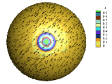
(a) Conservational laws

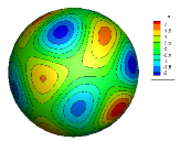
(b) Diffusion equation

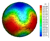
(c) Shallow water equations

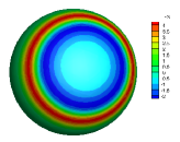
(d) Maxwell’s equations

Figure 4: Numerical simulation of the MMF scheme in Nektar++ for several partial differential equations solved on the sphere.

Modern scientific computation faces unprecedented demands on computational simulation in multidimensional complex domains composed of various materials. Examples of this include solving shallow water equations on a rotating sphere for weather prediction, incorporating biological anisotropic properties of cardiac and neural tissue for clinical diagnosis, and simulating the electromagnetic wave propagation on metamaterials for controlling electromagnetic nonlinear phenomena. All of these examples require the ability to solve PDEs on manifolds embedded in higher-dimensional domains. The method of moving frames (MMF) implemented in Nektar++ is a novel numerical scheme for solving such computational simulations in geometrically-complex domains.

Moving frames, principally developed by Élie Cartan in the context of Lie groups in the early 20th century [56, 57, 58], are orthonormal vector bases that are constructed at every grid point in the discrete space of a domain $\Omega$. Moving frames are considered as an ‘independent’ coordinate system at each grid point, and can be viewed as a dimensional reduction because the number of moving frames corresponds to dimensionality, independent of the space dimension. In this sense, ‘moving’ does not mean that the frames are time-dependent, but are different in a pointwise sense: i.e. if a particle travels from one point to the other, then it may undergo a different frame, which looks like a series of ‘moving’ frames. More recently this approach has been adapted more practical and computational purposes, mostly in computer vision [59, 60, 61] and medical sciences [62].

Building such moving frames is easily achieved by differentiating the parametric mapping $\mathbf{x}$ of a domain element $\Omega_{e}$ with respect to each coordinate axis of a standard reference space, followed by a Gram-Schmidt orthogonalization process. We obtain orthonormal vector bases, denoted as $\mathbf{e}^{i}$, with the following properties:

$$\mathbf{e}^{i}\cdot\mathbf{e}^{j}=\delta^{i}_{j},\leavevmode\nobreak\ \leavevmode\nobreak\ \leavevmode\nobreak\ \leavevmode\nobreak\ \leavevmode\nobreak\ \|\mathbf{e}^{i}\|=1,\leavevmode\nobreak\ \leavevmode\nobreak\ \leavevmode\nobreak\ \leavevmode\nobreak\ 1\leq i,j\leq 3,$$

where $\delta^{i}_{j}$ denotes the Kronecker delta. Moreover, the moving frames are constructed such that they are differentiable within each element and always lie on the tangent plane at each grid point. These two intrinsic properties of frames implies that any vector or the gradient can be expanded on moving frames as follows:

$$\mathbf{v}=v^{1}\mathbf{e}^{1}+v^{2}\mathbf{e}^{2},\leavevmode\nobreak\ \leavevmode\nobreak\ \leavevmode\nobreak\ \leavevmode\nobreak\ \leavevmode\nobreak\ \leavevmode\nobreak\ \nabla u=u^{1}\mathbf{e}^{1}+u^{2}\mathbf{e}^{2}.$$

Applying this expansion to a given PDE enables us to re-express it with moving frames on any curved surface. Then, the weak formulation of the PDE with moving frames, called the MMF scheme, on a curved surface is similar to the scheme in the Euclidean space, in the sense that it contains no metric tensor or its derivatives and it does not require the construction of a continuous curved axis in $\Omega$ which often produces geometric singularities. This is a direct result of the fact that moving frames are locally Euclidean. However, the numerical scheme with moving frames results in the accurate solutions of PDEs on any types of surfaces such as spheres, irregular surfaces, or non-convex surfaces. Some examples of simulations that can be achieved under this approach include conservational laws [63], the diffusion equation [64], shallow water equations (SWEs) [65], and Maxwell’s equations [66]. Representative results from Nektar++ for these equations on the surface of a sphere are shown in Figure 4.

Moreover, moving frames have been proven to be efficient for other geometrical realizations, such as the representation of anisotropic properties of media on complex domains [64], incorporating the rotational effect of any arbitrary shape [65], and adapting isotropic upwind numerical flux in anisotropic media [66]. The accuracy of the MMF scheme with the higher-order curvilinear meshes produced by NekMesh, described in Section 5.1, is reported to be significantly improved for a high $p$ and conservational properties such as mass and energy after a long time integration, whereas the accuracy of the MMF-SWE scheme on NekMesh is presented to be the best among all the previous SWE numerical schemes [67]. Ongoing research topics on moving frames are to construct the connections of frames, to compute propagational curvature, and finally to build an Atlas (a geometric map with connection and curvature) in order to provide a quantitative measurement and analysis of a flow on complex geometry. Examples of ongoing research topics in this area are include electrical activation in the heart [68] and fiber tracking of white matter in the brain.

4.2 Spatially-variable polynomial order

An important difficulty in the simulation of flows of practical interest is the wide range of length- and time-scales involved, especially in the presence of turbulence. This problem is aggravated by the fact that in many cases it is difficult to predict where in the domain an increase in the spatial resolution is required before conducting the simulation, while performing a uniform refinement across the domain is computationally prohibitive. Therefore, in dealing with these types of flows, it is advantageous to have an adaptive approach which allows us to dynamically adjust the spatial resolution of the discretisation both in time and in space.

Within the spectral/$hp$ element framework, it is possible to refine the solution following two different routes. $h$-refinement consists of reducing the size of the elements as would be done in low-order methods. This is the common approach for the initial distribution of degrees of freedom over the domain, with the computational mesh clustering more elements in regions where small scales are expected to occur, such as boundary layers. The other route is $p$-refinement (sometimes called $p$-enrichment), where the spatial resolution is increased by using a higher polynomial order to represent the solution. As discussed in [69], the polynomial order can be easily varied across elements in the spectral/$hp$ element method if the expansion basis is chosen appropriately. In particular if a basis admits a boundary-interior decomposition, such as the modified $C^{0}$ basis described in section 2 or the classical Lagrange interpolant basis, then the variation in polynomial order can be built into the assembly operation between interconnected elements. This allows for a simple approach to performing local refinement of the solution, requiring only the adjustment of the polynomial order in each element.

With this in mind, an adaptive polynomial order procedure has been implemented in Nektar++, with successful applications to simulations of incompressible flows. The basic idea in this approach is to adjust the polynomial order during the solution based on an element-local error indicator. The approach we used is similar to that demonstrated for shock capturing in [70], whereby oscilliatory behaviour in the solution field is detected by an error sensor on each element $\Omega_{e}$ calculated as

$$S_{e}=\frac{\|u_{P}-u_{P-1}\|^{2}_{2}}{\|u_{P}\|^{2}_{2}},$$

where $u_{P}$ is the solution obtained for the $u$ velocity using the current polynomial order $P$, $u_{P-1}$ is the projection of this solution to a polynomial of order $P-1$ and $\|\cdot\|_{2}$ denotes the $L^{2}$ norm. After each $n_{\text{steps}}$ time-steps, this estimate is evaluated for each element. For elements where the estimate of the error is above a chosen threshold, $P$ is incremented by one, whereas in elements with low error $P$ is decremented by one, respecting minimum and maximum values for $P$. The choice of $n_{\text{steps}}$ is critical for the efficiency of this scheme, since it has to be sufficiently large to compensate for the costs of performing the refinement over a large number of time-steps, yet small enough to adjust to changes in the flow. More details on this adaptive procedure for adjusting the polynomial order, as well as its implementation in both CG and DG regimes, are found in [69].

An example of an application of the adaptive polynomial order procedure is presented in Figure 5, showing the spanwise vorticity and polynomial order distributions for a quasi-3D simulation of the incompressible flow around a NACA 0012 profile at Reynolds number $Re=\numprint{50000}$ and angle of attack $\alpha=6^{\circ}$. The session files to generate this data can be found in Example 17. It is clear that the regions with transition to turbulence and the boundary layers are resolved using the largest polynomial order allowed, while regions far from the airfoil use a low polynomial order. This way, the scheme succeeds in refining the discretisation in the more critical regions where small scales are present, without incurring in the large computational costs that would be required to uniformly increase the polynomial order. More simply stated, it is possible to specify different polynomial order in the quadrilateral elements (typically used in boundary layer discretisation) and the triangle elements (typically used to fill the outer volume). As a final point, we note that the use of variable polynomial order is not limited to quasi-3D simulations; both CG and DG discretisations fully support all element shape types in 2D and 3D, with parallel implementations (including frequently used preconditioners) also supporting this discretisation option.

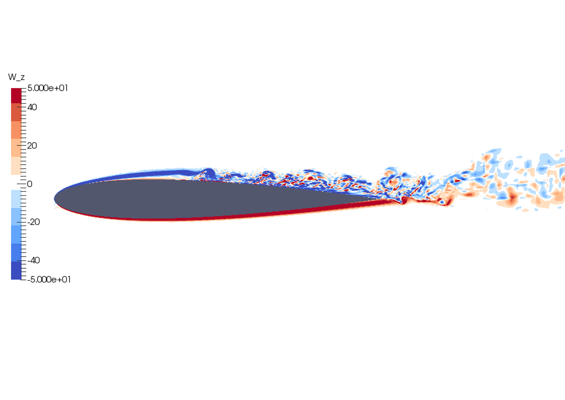
(a) Spanwise vorticity

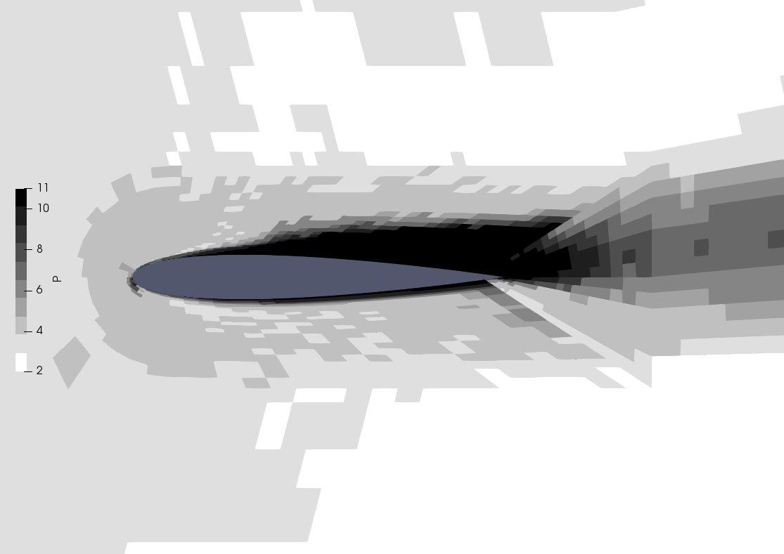
(b) Polynomial order

Figure 5: Polynomial order and vorticity distributions obtained with simulation using adaptive polynomial order for the flow around a NACA 0012 profile with $Re=\numprint{50000}$ and $\alpha=6^{\circ}$. Taken from [69].

4.3 Global mapping

Even though the spectral/$hp$ element spatial discretization allows us to model complex geometries, in some cases it can be advantageous to apply a coordinate transformation for solving problems that lie in a coordinate system other than the Cartesian frame of reference. This is typically the case when the transformed domain possesses a symmetry; this allows us to solve the equations more efficiently by compensating for the extra cost of applying the coordinate transformation. Examples of this occur when a transform can be used to map a non-homogeneous geometry to a homogeneous geometry in one or more directions. This makes it possible to use the cheaper quasi-3D approach, where this direction is discretized using a Fourier expansion, and also for problems with moving boundaries, where we can map the true domain to a fixed computational domain, avoiding the need for recomputing the system matrices after every time-step.

The implementation of this method was achieved in two parts. First, a new library called GlobalMapping was created, implementing general tensor calculus operations for several types of transformations. Even though it would be sufficient to consider just a completely general transformation, specific implementations for particular cases of simpler transformations are also included in order to improve the computational efficiency, since in these simpler cases many of the metric terms are trivial. In a second stage, the incompressible Navier-Stokes solver was extended, using the functionality of the GlobalMapping library to implement the methods presented in [71]. Some examples of applications are given in [72, 73]. Embedding these global mappings at the library level allows similar techniques to be introduced in other solvers in the future.

Figure 6 presents an example of the application of this technique, indicating the recirculation regions (i.e. regions where the streamwise velocity is negative) for the flow over a wing with spanwise waviness. In this case, the coordinate transformation removes the waviness from the wing, allowing us to treat the transformed geometry with the quasi-3D formulation. It is important to note that this technique becomes unstable as the waviness amplitude becomes too large. The fully explicit mapping is more sensitive to instability than the semi-implicit mapping as discussed in [71]. However, in cases where it can be successfully applied, it leads to significant gains in terms of computational cost when compared against a fully 3D implementation. The session files used in this example can be found in Example 18.

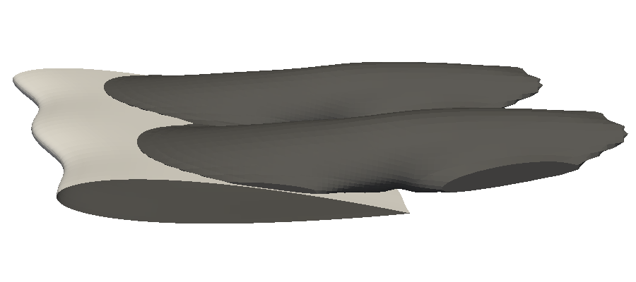
Figure 6: Time-averaged streamwise reversing regions for incompressible flow over a wing with spanwise waviness with $Re=\numprint{1000}$ and $\alpha=12^{\circ}$.

5 Applications

In this section, we demonstrate some of the new features provided in our new release, with a focus on application areas.

5.1 NekMesh

In the previous publication [33], we briefly outlined the MeshConvert utility, which was designed to read various external file formats and perform basic processing and format conversion. In the new release of Nektar++, MeshConvert has been transformed into a new tool, called NekMesh, which provides a series of tools for both the generation of meshes from an underlying CAD geometry, as well as the manipulation of linear meshes to make them suitable for high-order simulations. While MeshConvert was dedicated to the conversion of external mesh file formats, the scope of NekMesh has been significantly broadened to become a true stand-alone high-order mesh generator.

The generation of high-order meshes in NekMesh follows an a posteriori approach proposed in [74]. We first generate a linear mesh using traditional low-order mesh generation techniques. We then add additional nodes along edges, faces and volumes to achieve a high-order polynomial discretisation of our mesh. In the text below, we refer to these additional nodes as ‘high-order’ nodes, as they do not change the topology of the underlying linear mesh, but instead deform it to fit a required geometry. In this bottom-up procedure, these nodes are first added on edges, followed by faces and finally the volume-interior. At each step, nodes are generated on boundaries to ensure a geometrically accurate representation of the model.

A key issue in this process, however, is ensuring that elements remain valid after the insertion of high-order nodes, as this process is highly sensitive to boundary curvature. A common example of this is in boundary layer mesh generation [75], where elements are typically extremely thin in order to resolve the high-shear of the flow near the wall. In this setting, naively introducing curvature into the element will commonly push one face of the element through another, leading a self-intersecting element and thus a mesh that is invalid for computation.

An important contribution of NekMesh to the high-order mesh generation community was presented in references [75, 76], where we alleviate this risk through the creation of a coarse, single element boundary layer mesh with edges orthogonal to the boundary. The thickness of the layer of elements gives enough room for a valid curving of the ‘macro’-elements. After creation of the high-order mesh, a splitting of these boundary elements can be performed using the isoparametric mapping between the reference space and the physical space. We then apply the original isoparametric mapping to construct new elements within the ‘macro’ element, thereby guaranteeing their validity. This ensures conservation of the validity and quality of subdivided elements while achieving very fine meshes. An example is shown in Figure 7 where the coarse boundary layer mesh of Figure 8 was split into five layers, using a geometric progression of growth rate $r=2$ in the thickness of each layer. The session files used to create the meshes for Figure 8 and 9 can be found in Example 20.

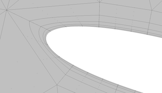
Figure 7: Example of split boundary layer mesh.

A complementary approach to avoid invalid or low quality high-order elements is to optimise the location of high-order nodes in the mesh. The approach proposed in [13, 77] of a variational framework for high-order mesh optimisation was implemented in NekMesh. In this approach, we consider the mesh to be a solid body, and define a functional based on the deformation of each high-order element. This functional can correspond to physical solid mechanics governing equations such as linear or non-linear elasticity, but also provides the possibility to accommodate arbitrary functional forms such as the Winslow equations within the same framework. Minimising this functional is then achieved through classical quasi-Newton optimisation methods with the use of analytic gradient functions, alongside a Jacobian regularisation technique to accomodate initially-invalid elements. As demonstrated in [13], the approach is scalable and allows the possibility to implement advanced features, such as the ability to slide nodes along a given constrained CAD curve or surface.

Along these lines, much of the development of NekMesh has focused on the access to a robust CAD system for CAD queries required for traditional meshing operations. Assuming that the CAD is watertight, we note that only a handful of CAD operations are required for mesh generation purposes. NekMesh therefore implements a lightweight wrapper around these CAD queries, allowing it to be interfaced to a number of CAD systems. By default, we provide an interface to the open-source OpenCASCADE library [78]. OpenCASCADE is able to read the STEP CAD file format, natively exported by most CAD design tools, and load it into the system. At the same time, the use of a wrapper means that users and developers of NekMesh are not exposed to the extensive OpenCASCADE API. Although OpenCASCADE is freely available and very well suited to simple geometries, it lacks many of the CAD healing tools required for more complex geometries of the type typically found in industrial CFD environments, which can frequently contain many imperfections and inconsistencies. However, the use of a lightweight wrapper means that other commerical CAD packages can be interfaced to NekMesh if available. To this end, we have implemented a second CAD interface to the commerical CFI CAD engine, which provides a highly robust interface and is described further in references [79, 39, 77].

While users are recommended to create their CAD models in a dedicated CAD software, export them in STEP format and load them in NekMesh, they also have the possibility to create their own simple two-dimensional models using one of two tools made available to them. The first tool is an automatic NACA aerofoil generator. With just three inputs – a NACA code, an angle of attack and dimensions of the bounding box – a geometry is generated and passed to the meshing software. An example is shown in Figure 8 of a mesh generated around a NACA 0012 aerofoil at an angle of attack of $\alpha=15^{\circ}$.

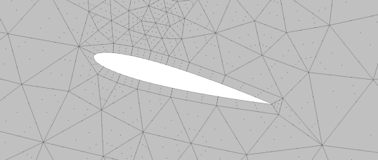
Figure 8: Example of mesh generated around a NACA 0012 aerofoil.

The other tool is based on the GEO geometry file format of the Gmsh [80] open source mesh generator. The GEO format is an intepreter for the procedural generation of geometries. NekMesh has been made capable to understand basic GEO commands, which gives the possibility to generate simple two-dimensional geometries. An example is shown in Figure 9 of a mesh generated around a T106C turbine blade: the geometry was created using a GEO script of lines and splines.

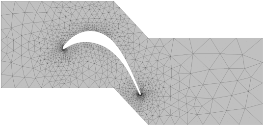
Figure 9: Example of mesh generated around a t106c turbine blade.

5.2 Acoustic solver

Time-domain computational aeroacoustics simulations are commonly used to model noise emission over wide frequency ranges or to augment flow simulations in hybrid setups. Compared with fully compressible flow simulations, they require less computational effort due to the reduced complexity of the governing equations and larger length scales [81]. However, due to the small diffusive terms, as well as the long integration times and distances required for these simulations, highly accurate numerical schemes are crucial for stability [82]. This numerical accuracy can be provided by spectral/$hp$ element methods, even on unstructured meshes in complex geometries, and hence Nektar++ provides a good candidate framework on which to build such an application code.

The latest release of Nektar++ includes a new AcousticSolver, which implements several variants of aeroacoustic models. These are formulated in a hyperbolic setting and implemented in a similar fashion to the compressible Euler and Navier-Stokes equations, encapsulated in Nektar++ inside the CompressibleFlowSolver. Following this implementation guideline, the AcousticSolver uses a discontinuous Galerkin spatial discretisation with modal or nodal expansions to model time-domain acoustic wave propagation in one, two or three dimensions. It implements the operators of the linearized Euler Equations (LEE) and the Acoustic Perturbation Equations 1 and 4 (APE-1/4) [83], both of which describe the evolution of perturbations around a base flow state. For the APE-1/4 operator, the system is defined by the hyperbolic equations

$$\frac{\partial p^{\mathrm{a}}}{\partial t}+\overline{c^{2}}\nabla\cdot\left(\overline{\rho}\bm{u}^{\mathrm{a}}+\overline{\bm{u}}\frac{p^{\mathrm{a}}}{\overline{c^{2}}}\right) =\dot{\omega}_{\mathrm{c}},$$ (4a)

$$\frac{\partial\bm{u}^{\mathrm{a}}}{\partial t}+\nabla\left(\overline{\bm{u}}\cdot\bm{u}^{\mathrm{a}}\right)+\nabla\left(\frac{p^{\mathrm{a}}}{\overline{\rho}}\right) =\dot{\bm{\omega}}_{\mathrm{m}},$$ (4b)

where $\bm{u}$ denotes the flow velocity, $\rho$ its density, $p$ its pressure and $c$ corresponds to the speed of sound. The quantities $\bm{u}^{a}$ and $p^{a}$ refer to the irrotational acoustic perturbation of the flow velocity and its pressure, with overline quantities such as $\overline{\bm{u}}$ denoting the time-averaged mean. The right-hand-side acoustic source terms terms $\dot{\omega}_{\mathrm{c}}$ and $\dot{\bm{\omega}}_{\mathrm{m}}$ are specified in the session file. This allows for the implementation of any acoustic source term formulation so that, for example, the full APE-1 or APE-4 can be obtained. In addition to using analytical expressions, the source terms and base flow quantities can be read from disk or transferred from coupled applications, enabling co-simulation with a driving flow solver. Both, LEE and APE support non-quiescent base flows with inhomogeneous speed of sounds. Accordingly, the Lax-Friedrichs and upwind Riemann solvers used in the AcousticSolver employ a formulation which is valid even for strong base flow gradients. The numerical stability can be further improved by optional sponge layers and suitable boundary conditions, such as rigid wall, farfield or white noise.

A recurring test case for APE implementations is the “spinning vortex pair” [84]. It is defined using two opposing vortices, that are each located at $r_{0}$ from the center $x_{1}=x_{2}=0$ of a square domain with edge length $-100\,r_{0}\leq x_{1,2}\leq 100\,r_{0}$. The vortices have a circulation of $\Gamma$ and rotate around the center at the angular frequency $\omega=\Gamma/4\pi r_{0}^{2}$ and circumferential Mach number $\mathit{Ma}_{r}=\Gamma/4\pi r_{0}c$. The resulting acoustic pressure distribution is shown in Figure 10(a) and was obtained on an unstructured mesh of 465 quadrilateral elements with a fifth order modal expansion ($P=5$). The session files used to generate this example can be found in Example 19. Along the black dashed line, the acoustic pressure shown in Figure 10(b) exhibits minor deviations from the analytical solution defined in [84], but is in excellent agreement with the results of the original simulation in [83]. The latter was based on a structured mesh with 19,881 nodes and employed a sponge layer boundary condition and spatial filtering to improve the stability. Due to the flexibility and numerical accuracy of the spectral/$hp$ method, a discretization with only 16,740 degrees of freedom was sufficient for this simulation, and no stabilization measures (e.g. SVV or filtering) were necessary to reproduce this result.

(a) Normalized acoustic pressure distribution at $t=1\text{s}$ with the mesh shown in light gray and the sampling line in a black dashed line.

(b) Normalized acoustic pressure along sample line, obtained with the AcousticSolver and analytical solution [84].

Figure 10: Normalized acoustic pressure for $\Gamma/(cr_{0})=1.0$ and $\mathit{Ma}_{r}=0.0795$ at $t=1\mathrm{s}$.

5.3 Fluid-Structure Interaction (FSI) and Vortex-Induced Vibration (VIV)

Fluid-structure interaction (FSI) modelling poses a great challenge for the accurate prediction of vortex-induced vibration (VIV) of long flexible bodies, as the full resolution of turbulent flow along their whole span requires considerable computational resources. This is particularly true in the case of large aspect-ratio bodies. Although 2D strip-theory-based modelling of such problems is much more computationally efficient, this approach is unable to resolve the effects of turbulent fluctuations on dynamic coupling of FSI systems [85, 86]. A novel strip model, which we refer to as ‘thick’ strip modelling, has been developed using the the Nektar++ framework in [87], whose implementation is supported within the incompressible Navier-Stokes solver. In this approach, a three-dimensional DNS model with a local spanwise scale is constructed for each individual strip. Coupling between strips is modelled implicitly through the structural dynamics of the flexible body.

In the ‘thick’ strip model, the flow dynamics are governed by a series of incompressible Navier-Stokes equations. The governing equations over a general local domain $\mathit{\Omega}_{n}$ associated with the $n$-th strip are written as

$${\partial{\mathbf{u}_{n}}\over{\partial t}}+({\mathbf{u}_{n}}\cdot\nabla){\mathbf{u}_{n}}=-\nabla p_{n}+{1\over Re}\nabla^{2}{\mathbf{u}_{n}}\quad\mbox{on}\quad\mathit{\Omega}_{n}$$ (5)

$$\nabla\cdot{\mathbf{u}_{n}}=0\quad\mbox{on}\quad\mathit{\Omega}_{n},$$ (6)

where the vector $\mathbf{u}_{n}=(u_{n},v_{n},w_{n})$ denotes the fluid velocity inside the $n$-th strip, with $p_{n}$ being the corresponding dynamic pressure and $Re$ the Reynolds number, which we assume to be constant across all strips. The governing equations are supplemented by boundary conditions of either Dirichlet or Neumann type. In particular, no-slip boundary conditions are applied to the wall of the body, and the velocity of the moving wall is imposed and determined from the transient solution of structural dynamics equations of motion. A linearized tensioned beam model is used to describe the structural dynamic behavior of the flexible body, which is expressed by the system

$$\rho_{c}{\partial^{2}{\bm{\eta}}\over{\partial t}^{2}}+{c}{\partial{\bm{\eta}}\over{\partial t}}-{T}{\partial^{2}{\bm{\eta}}\over{\partial z}^{2}}+{EI}{\partial^{4}{\bm{\eta}}\over{\partial z}^{4}}={\bf f}.$$ (7)

In the above, $\rho_{c}$ is the structural mass per unit length, $c$ is the structural damping per unit length, $T$ is the tension and $EI$ is the flexural rigidity. $\mathbf{f}$ denotes the vector of hydrodynamic force per unit length exerted on the body’s wall and $\bm{\eta}$ is the structural displacement vector.

Homogeneity is imposed in the spanwise direction to the local flow within individual strips, under the assumption that the width of the strips is much shorter with respect to the oscillation wavelength of excited higher-order modes of the flexible body. This therefore enables the use of the computationally-efficient quasi-3D approach discussed in previous sections within each strip domain, in which two-dimensional spectral elements with piecewise polynomial expansions are used in the $(x,y)$ plane and Fourier expansions are used in the homogeneous $z$ direction. This also requires the assumption of a spanwise oscillation of the flexible body with respect to its full-length scale. As a consequence, the motion variables and fluid forces are expressed as a complex Fourier series, and the tensioned beam model is decoupled into a set of ordinary differential equations, which can be solved simply by a second-order Newmark-$\beta$ method [88]. A partitioned approach is adopted to solve the coupled FSI system, in which coordinate mapping technique discussed in Section 4.3 is implemented for the treatment of the moving wall [71].

To illustrate the application of this modelling approach, VIV of a long flexible cylinder with an aspect ratio of $32\pi$ which is pinned at both ends is simulated at $Re=\numprint{3900}$, with 16 thick strips allocated evenly along the axial line of the cylinder. The instantaneous spanwise wake structure is visualized by the vortex-identification of Q-criterion in Figure 11. As the figure demonstrates, the distribution of vortex shedding illustrates that a second harmonic mode is excited along the spanwise length and the turbulent structure is captured well in the local domain of the strips. This emphasises the convincing advantage of providing highly-resolved description of hydrodynamics involved in the FSI process. The session files used to run this simulation can be found in Example 21.

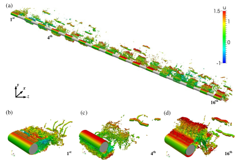
Figure 11: Instantaneous vortex shedding visualized by the vortex-identification of Q-criterion (iso-surfaces of the Q-value= $[-5,5]$) in body-fitted coordinates: (a) full domain view and zoom-in view of (b) first strip; (c) fourth strip and (d) 16th strip.

5.4 Aeronautical applications

CFD is now an indispensable tool for the design of aircraft engines, and it has become commonplace in the design guidance of new technologies and products [89]. In order for CFD to be effectively adopted in industry, validation and verification is required over a broad design space. This is challenging for a number of reasons, including the range of operating conditions (i.e. Reynolds numbers, Mach numbers, temperatures and pressures), the complexity of industrial geometries (including uncertainty due to manufacturing variations) and their relative motion (i.e. rotor-stator interactions). Even though RANS continues to be the backbone of CFD-based design, the recent development of high-order unstructured solvers and high-order unstructured meshing algorithms, combined with the lowering cost of HPC infrastructures, has the potential to allow for the introduction of high-fidelity transient simulations using large-eddy or direct numerical simulations (LES/DNS) in the design loop, taking the role of a virtual wind tunnel.

As part of our effort to bridge the gap between academia and industry, we have been developing the expertise to analyse turbomachinery cases of industrial interest using Nektar++. A key problem to overcome in these cases is the sensitivity of these simulations to variations in spatial resolution, which requires the use of stabilisation techniques in order to improve robustness. Nektar++ makes use of the spectral vanishing viscosity (SVV) method, originally introduced for the Fourier spectral method by Tadmor [90]. SVV is a model-free stabilization technique that acts at the subgrid-scale level and allows for exponential convergence properties to be conserved in sufficiently resolved simulations. Recent developments in this area have focused on a new SVV kernel by Moura et al. [3], which replicates the desirable dispersion and diffusion properties of DG schemes and does not require the manual tuning of parameters found in the classical SVV formulation. More specifically, the dissipation curves of the CG scheme of order $P$ were compared to those of DG order $P-2$, and the DG kernel was determined from minimization of the point-wise $L_{2}$ norm between these curves. SVV stabilization is combined with spectral/hp dealiasing [29] to eliminate errors arising from the integration of non-linear terms.

A T106A low pressure turbine vane was investigated at moderate regime ($Re=\numprint{88450}$), and the convergence properties of the main flow statistics were extensively explored with the aim of developing a set of best practices for the use of spectral/hp element methods as a high-fidelity digital twin [91]. The velocity correction scheme of [92] implemented in the IncNavierStokesSolver is adopted, using the quasi-3D approach discussed in the previous sections and Taylor-Hood type elements in 2D (where spaces of order $P$ polynomials on each element are used for the velocity components, and $P-1$ for pressure). Uniform inflow velocity is combined with pitchwise periodicity and high-order outflow boundary conditions [93]. Numerical stability is ensured by employing SVV with the DG kernel in the $x$-$y$ planes, and the traditional exponential kernel for the spanwise Fourier direction. A representation of the vortical structures is shown in Figure 12: transition to turbulence takes place only in the final portion of the suction surface, where the separated shear layer rolls up due to Kevin-Helmoltz instability. The separation bubble remains open and merges into the trailing edge wake, giving rise to large-scale vortical structures. This work was conducted with clean inflow conditions to isolate the effect of the numerical setup on the various flow statistics. However, turbomachinery flows are highly turbulent: subsequent work focused on the treatment of flow disturbances to reproduce more accurately a realistic environment [94]. With this aim, a localised synthetic momentum forcing was introduced in the leading edge region to cause flow symmetry breakdown on the suction surface, and promote anticipated transition to turbulence. This approach yields an improvement in the agreement with experimental data, with no increase in the computational cost.

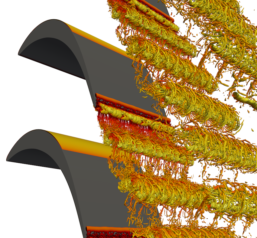
Figure 12: Instantaneous isosurfaces of $Q$-criterion ($Q=500$) contoured by velocity magnitude, showing the vortical structures evolving on the suction surface and in the wake of a T106A cascade. The computational domain is replicated in the spanwise and pitchwise directions for visual clarity.

With the intent of being able to tackle cases in which compressibility effects are not negligible, there has been an effort in validating the CompressibleFlowSolver for shock-wave boundary layer interaction (SWBLI) configurations. This solver, described in our previous publication [33], formulates the compressible Navier-Stokes equations in their conservative form, discretised using a DG scheme and explicit timestepping methods. In order to regularize the solution in the presence of discontinuities, the right hand side of the Navier-Stokes equations is augmented with a Laplacian viscosity term of the form $\nabla\cdot\left(\varepsilon\nabla\mathbf{q}\right)$, where $\mathbf{q}$ is the vector of conserved variables, and $\varepsilon$ is a spatially-dependent diffusion term that is defined on each element as

$$\varepsilon=\varepsilon_{0}\frac{h}{p}\lambda_{\text{max}}S.$$

Here, $\varepsilon_{0}$ is a $O(1)$ constant, $\lambda_{\text{max}}$ is the maximum local characteristic speed, $h$ is a reference length of the element, $p$ its polynomial order, and $S$ a discontinuity sensor value using the formulation of [70]. To benchmark this approach in the context of SWBLI problems, we consider a laminar problem studied experimentally and numerically in [95]. Several authors have studied this SWBLI with slightly different free stream conditions; here we follow the physical parameters used by [96], where we select a free-stream Mach number $Ma=2.15$, shock angle $\beta=30.8^{\circ}$, a stagnation pressure $p_{0}=1.07\times 10^{4}$ Pa, a stagnation temperature of $T_{0}=293K$, a Reynolds number $Re=10^{5}$ (referred to the inviscid shock impingement location $x_{\text{sh}}$ measured from the plate leading edge), and a Prandtl number $Pr=0.72$. Unlike [96], the leading edge is not included in the simulations. The inflow boundary is located at $x=0.3x_{\text{sh}}$ where the analytical compressible boundary layer solution of [97] is imposed. The session files used in this example can be found in Example 22. At the inlet, the Rankine-Hugoniot relations that describe the incident shock are superimposed over the compressible boundary layer solution. At the top boundary we impose the constant states corresponding to inviscid post incident shock wave state. At the outlet in the subsonic part of the boundary layer a pressure outlet is imposed based on the inviscid post reflected state conditions. All boundary conditions are imposed in a weak sense through a Riemann solver, as described in [98], and use a coarse grid of $60\times 40$ quadrilateral elements at order $p=3$. For illustrative purposes, Figure 13 shows a snapshot of the Mach number field. For a more quantitative comparison, Figure 14 compares the skin friction coefficient with those from [99] and [96], which is in fair agreement with the results of [96].

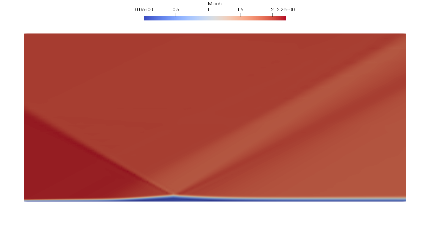
Figure 13: Mach number field of SWBLI test case ($60\times 40$ quadrilateral elements, $p=3$); configuration based on [95].

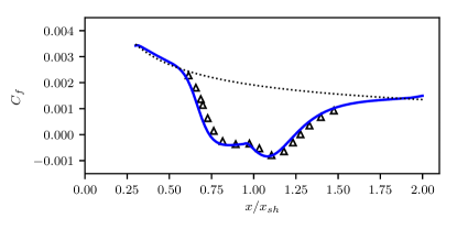
Figure 14: Skin friction coefficient for the SWBLI test case: blue line Nektar++ ($60\times 40$ quadrilateral elements, $p=3$); triangles are from [96]; dotted line is empirical solution by [99].

6 Availability

Nektar++ is open-source software, released under the MIT license, and is freely available from the project website (https://www.nektar.info/). The git repository is freely accessible and can be found at https://gitlab.nektar.info/. Discrete releases are made at milestones in the project and are available to download as compressed tar archives, or as binary packages for a range of operating systems. These releases are considered to contain relatively complete functionality compared to the repository master branch. Docker container images are also available for these releases and the latest build of master, as well as a Jupyter notebook that contains the Python interface of Section 3.5. These can be found on Dockerhub under the repositories nektarpp/nektar and nektarpp/nektar-workbook respectively.

7 Conclusions

In this paper, we have reviewed the latest features and enhancements of the Nektar++ version 5.0 release. A key theme of our work in this release has been to evolve the fundamental design of the software detailed in our previous publication [33], towards providing an enabling tool for efficient high-fidelity simulations in various scientific areas. To this end, this latest version of Nektar++ provides a complete pipeline of tools: from pre-processing with NekMesh and a new parallel I/O interface for mesh and field representations; new solvers and improvements to existing ones through numerical developments such as spatially variable polynomial order and the global mapping technique; to parallel post-processing and in-situ processing with the FieldConvert utility developments. This gives scientific end-users a tool to enable efficient high-fidelity simulations in a number of fields, such as the applications we discuss in Section 5.

Although this version represents a major milestone in the development of Nektar++, there is still clear scope for future work. A particular area of focus remains the efficient use of many-core CPU and GPU systems, recognising that optimisation and performance on an increasingly diverse range of hardware presents a major challenge. Initial research in this area has investigated the use of matrix-free methods as a potential route towards fully utilising computational hardware even on unstructured grids, by combining efficient sum factorisation techniques and the tensor-product basis for unstructured elements presented in [36]. From the perspective of code maintainability, we have also investigated various performance-portable programming models in the context of mesh generation [100] and implicit solvers [101]. Looking towards the next major release of Nektar++, we envision the use of these studies as a guideline to implementing efficient operators for the spectral/$hp$ element method, whilst retaining ease of use for the development of increasingly efficient solvers.

Acknowledgements

The development of Nektar++ has been supported by a number of funding agencies including the Engineering and Physical Sciences Research Council (grants EP/R029423/1, EP/R029326/1 EP/L000407/1, EP/K037536/1, EP/K038788/1, EP/L000261/1, EP/I037946/1, EP/H000208/1, EP/I030239/1, EP/H050507/1, EP/D044073/1, EP/C539834/1), the British Heart Foundation (grants FS/11/22/28745 and RG/10/11/28457), the Royal Society of Engineering, European Union FP7 and Horizon 2020 programmes (grant nos. 265780, 671571 and 675008), McLaren Racing, the National Science Foundation (IIS-0914564, IIS-1212806 and DMS-1521748), the Army Research Office (W911NF-15-1-0222), the Air Force Office of Scientific Research and the Department of Energy. HX acknowledges support from the NSF Grants 91852106 and 91841303. SC acknowledges the support of the National Research Foundation of Korea (No. 2016R1D1A1A02937255). KL acknowledges the Seventh Framework Programme FP7 Grant No. 312444 and German Research Foundation (DFG) Grant No. JA 544/37-2.

Appendix A Supplementary material

File: user-guide.pdf

Figure 15: User guide for Nektar++ detailing compilation, installation, input format and usage, including examples.

File: insitu.zip

Figure 16: Nektar++ input files for simulating flow past a cylinder at $Re=\numprint{80}$ using IncNavierStokesSolver. This example uses the HDF5 input format described in Section 3.1 and the in-situ processing facilities of Section 3.2 to generate an animation of the vorticity field and show the von Kármán vortex shedding in this regime.

File: adaptiveOrder.zip

Figure 17: Nektar++ input files for simulating flow over a NACA0012 wing at $Re=\numprint{50000}$ using IncNavierStokesSolver. This example uses an adaptive-in-time polynomial order described in Section 4.2 to increase efficiency of the simulation when compared to a spatially-constant polynomial order.

File: wavyWing.zip

Figure 18: Nektar++ input files for simulating flow over a wavy NACA0012 wing at $Re=\numprint{1000}$ using IncNavierStokesSolver. This example uses the mapping technique described in Section 4.3 to perform simulations in a quasi-3D setting.

File: acoustic.zip

Figure 19: Nektar++ input files for simulating the spinning vortex pair using the AcousticSolver of Section 5.2 at a polynomial order of $P=5$, accelerated using the Collections library described in Section 3.3.

File: meshGen.zip

Figure 20: NekMesh input files for a NACA0012 aerofoil section and T106C turbine blade geometry outlined in Section 5.1.

File: vivCylFlow.zip

Figure 21: Nektar++ input files for simulating flow over a flexible cylinder $Re=\numprint{3900}$ using the IncNavierStokesSolver. This example uses the the thick strip model outlined in Section 5.3 to reduce computational cost against a full 3D simulation.

File: shockBL.zip

Figure 22: Nektar++ input files for simulating a shock boundary-layer interaction test case, at a Reynolds number $Re=10^{5}$, Mach number $Ma=\numprint{2.15}$ and shock angle $\beta=\numprint{30.8}^{\circ}$ as outlined in Section 5.4.

References

- [1] R. C. Moura, G. Mengaldo, J. Peiró, S. Sherwin, Journal of Computational Physics 330 (2017) 615–623.
- [2] R. C. Moura, G. Mengaldo, J. Peiró, S. J. Sherwin, An LES setting for DG-based implicit LES with insights on dissipation and robustness, in: Spectral and High Order Methods for Partial Differential Equations ICOSAHOM 2016, Springer, 2017, pp. 161–173.
- [3] G. Mengaldo, R. Moura, B. Giralda, J. Peiró, S. Sherwin, Computers & Fluids 169 (2018) 349–364.
- [4] G. Mengaldo, D. De Grazia, R. C. Moura, S. J. Sherwin, Journal of Computational Physics 358 (2018) 1–20.
- [5] P. Fernandez, R. C. Moura, G. Mengaldo, J. Peraire, Computer Methods in Applied Mechanics and Engineering 346 (2019) 43–62.
- [6] P. E. Vos, S. J. Sherwin, R. M. Kirby, Journal of Computational Physics 229 (13) (2010) 5161–5181.
- [7] C. D. Cantwell, S. J. Sherwin, R. M. Kirby, P. H. J. Kelly, Computers & Fluids 43 (2011) 23–28.
- [8] C. D. Cantwell, S. J. Sherwin, R. M. Kirby, P. H. J. Kelly, Math. Mod. Nat. Phenom. 6 (2011) 84–96.
- [9] G. J. Gassner, SIAM Journal on Scientific Computing 35 (3) (2013) A1233–A1253.
- [10] G. Mengaldo, D. De Grazia, P. E. Vincent, S. J. Sherwin, Journal of Scientific Computing 67 (3) (2016) 1272–1292.
- [11] G. Mengaldo, Ph.D. dissertation (2015).
- [12] G. E. Karniadakis, S. J. Sherwin, Spectral/hp element methods for CFD, Oxford University Press, 2005.
- [13] M. Turner, J. Peiró, D. Moxey, Computer-Aided Design 103 (2018) 73–91.
- [14] P. Fischer, J. Kruse, J. Mullen, H. Tufo, J. Lottes, S. Kerkemeier, Argonne National Laboratory, Mathematics and Computer Science Division, Argonne, IL, see https://nek5000. mcs. anl. gov/index. php/MainPage (2008).
- [15] H. M. Blackburn, S. Sherwin, Journal of Computational Physics 197 (2) (2004) 759–778.
- [16] H. M. Blackburn, D. Lee, T. Albrecht, J. Singh, Computer Physics Communications 245 (2019) 106804.
- [17] W. Bangerth, R. Hartmann, G. Kanschat, ACM Transactions on Mathematical Software (TOMS) 33 (4) (2007) 24.
- [18] F. Hindenlang, G. J. Gassner, C. Altmann, A. Beck, M. Staudenmaier, C.-D. Munz, Computers & Fluids 61 (2012) 86–93.
- [19] G. J. Gassner, A. R. Winters, D. A. Kopriva, Journal of Computational Physics 327 (2016) 39–66.
- [20] F. X. Giraldo, M. Restelli, Journal of Computational Physics 227 (8) (2008) 3849–3877.
- [21] D. S. Abdi, F. X. Giraldo, Journal of Computational Physics 320 (2016) 46–68.
- [22] F. Witherden, A. Farrington, P. Vincent, Computer Physics Communications 185 (2014) 3028–3040. doi:10.1016/j.cpc.2014.07.011.
- [23] H. T. Huynh, A flux reconstruction approach to high-order schemes including discontinuous Galerkin methods, in: 18th AIAA Computational Fluid Dynamics Conference, 2007, p. 4079.
- [24] Y. Allaneau, A. Jameson, Computer Methods in Applied Mechanics and Engineering 200 (49-52) (2011) 3628–3636.
- [25] A. Dedner, R. Klöfkorn, M. Nolte, M. Ohlberger, Computing 90 (3-4) (2010) 165–196.
- [26] A. Bolis, C. D. Cantwell, D. Moxey, D. Serson, S. Sherwin, Computer Physics Communications 206 (2016) 17–25.
- [27] P. E. Vos, C. Eskilsson, A. Bolis, S. Chun, R. M. Kirby, S. J. Sherwin, International Journal of Computational Fluid Dynamics 25 (3) (2011) 107–125.
- [28] C. D. Cantwell, S. Yakovlev, R. M. Kirby, N. S. Peters, S. J. Sherwin, Journal of Computational Physics 257 (2014) 813–829.
- [29] G. Mengaldo, D. De Grazia, D. Moxey, P. E. Vincent, S. Sherwin, Journal of Computational Physics 299 (2015) 56–81.
- [30] A. R. Winters, R. C. Moura, G. Mengaldo, G. J. Gassner, S. Walch, J. Peiro, S. J. Sherwin, Journal of Computational Physics 372 (2018) 1–21.
- [31] R. M. Kirby, S. J. Sherwin, Computer Methods in Applied Mechanics and Engineering 195 (23-24) (2006) 3128–3144.
- [32] J.-E. W. Lombard, D. Moxey, S. J. Sherwin, J. F. Hoessler, S. Dhandapani, M. J. Taylor, AIAA Journal 54 (2) (2015) 506–518.
- [33] C. D. Cantwell, D. Moxey, A. Comerford, A. Bolis, G. Rocco, G. Mengaldo, D. de Grazia, S. Yakovlev, J.-E. Lombard, D. Ekelschot, B. Jordi, H. Xu, Y. Mohamied, C. Eskilsson, B. Nelson, P. Vos, C. Biotto, R. M. Kirby, S. J. Sherwin, Computer Physics Communications 192 (2015) 205–219. doi:10.1016/j.cpc.2015.02.008.
- [34] H. Xu, C. D. Cantwell, C. Monteserin, C. Eskilsson, A. P. Engsig-Karup, S. J. Sherwin, Journal of Hydrodynamics 30 (1) (2018) 1–22.
- [35] M. Dubiner, Journal of Scientific Computing 6 (4) (1991) 345–390.
- [36] S. J. Sherwin, G. E. Karniadakis, Computer Methods in Applied Mechanics and Engineering 123 (1-4) (1995) 189–229.
- [37] M. G. Duffy, SIAM Journal on Numerical Analysis 19 (6) (1982) 1260–1262.
- [38] F. Bassi, S. Rebay, Journal of Computational Physics 138 (2) (1997) 251–285.
- [39] J. Marcon, J. Peiró, D. Moxey, N. Bergemann, H. Bucklow, M. Gammon, A semi-structured approach to curvilinear mesh generation around streamlined bodies, in: AIAA Scitech 2019 Forum, American Institute of Aeronautics and Astronautics, Reston, Virginia, 2019, pp. 1725–. doi:10.2514/6.2019-1725.
- [40] D. Moxey, C. D. Cantwell, R. M. Kirby, S. J. Sherwin, Comput. Meth. Appl. Mech. Eng. 310 (2016) 628–645. doi:10.1016/j.cma.2016.07.001.
- [41] D. Moxey, R. Amici, R. M. Kirby, Efficient matrix-free high-order finite element evaluation for simplicial elements, under review in SIAM J. Sci. Comp. (2019).
- [42] S. Yakovlev, D. Moxey, S. J. Sherwin, R. M. Kirby, Journal of Scientific Computing 67 (1) (2016) 192–220.
- [43] B. Cockburn, C.-W. Shu, SIAM Journal on Numerical Analysis 35 (6) (1998) 2440–2463.
- [44] M. Folk, G. Heber, Q. Koziol, E. Pourmal, D. Robinson, An overview of the HDF5 technology suite and its applications, in: Proceedings of the EDBT/ICDT 2011 Workshop on Array Databases, ACM, 2011, pp. 36–47.
- [45] M. Bareford, N. Johnson, M. Weiland, Improving Nektar++ IO Performance for Cray XC Architecture, in: Cray User Group Proceedings, Stockholm, Sweden, 2018.
- [46] C. Chevalier, F. Pellegrini, Parallel Computing 34 (6-8) (2008) 318–331.
- [47] W. J. Schroeder, B. Lorensen, K. Martin, The visualization toolkit: an object-oriented approach to 3D graphics, Kitware, 2004.
- [48] J. Ahrens, B. Geveci, C. Law, The visualization handbook 717 (2005).
- [49] K. Lackhove, Hybrid Noise Simulation for Enclosed Configurations, Doctoral thesis, Technische Universität Darmstadt (2018).
- [50] M. Germano, Physics of Fluids 29 (6) (1986) 1755. doi:10.1063/1.865649.
- [51] A. Refloch, B. Courbet, A. Murrone, C. Laurent, J. Troyes, G. Chaineray, J. B. Dargaud, F. Vuillot, AerospaceLab (2011).
- [52] F. Duchaine, S. Jauré, D. Poitou, E. Quémerais, G. Staffelbach, T. Morel, L. Gicquel, Computational Science & Discovery 8 (1) (7 2015). doi:10.1088/1749-4699/8/1/015003.
- [53] D. Abrahams, R. W. Grosse-Kunstleve, O. Overloading, CC Plus Plus Users Journal 21 (7) (2003) 29–36.
- [54] P. Peterson, International Journal of Computational Science and Engineering 4 (4) (2009) 296–305.
- [55] D. M. Beazley, et al., SWIG: An easy to use tool for integrating scripting languages with C and C++, in: Tcl/Tk Workshop, 1996, p. 43.
- [56] Élie Cartan, Riemannian geometry in an orthogonal frame, World Scientific Pub. Co. Inc., 2002.
- [57] Élie Cartan, Geometry of Riemannian spaces, Math. Sci. Press, 2001.
- [58] Élie Cartan, La théorie des groupes finis et continus et la géométrie différentiellle traitees par la méthode du repère mobile, Gauthier-Villars, 1937.
- [59] M. Fels, P. J. Olver, Acta Appl. Math. 51 (2) (1998) 161–213.
- [60] P. J. Olver, Moving frames – in geometry, algebra, computer vision, and numerical analysis. foundations of computational mathematics, in: London Math. Soc. Lecture Note Ser., Cambridge Univ. Press, 2001, pp. 267–297.
- [61] O. Faugeras, Cartan’s moving frame method and its application to the geometry and evolution of curves in the euclidean, affine and projective planes, in: J. L. Mundy, A. Zisserman, D. Forsyth (Eds.), Lecture Notes in Computer Science, Vol. 825, Springer, 1994.
- [62] E. Piuze, J. Sporring, K. Siddiqi, Moving frames for hear fiber reconstruction, in: S. Ourselin, D. Alexander, D. Westin (Eds.), Lecture Notes in Computer Science book series, Vol. 9123, Springer, 2015.
- [63] S. Chun, Journal of Scientific Computing 53 (2) (2012) 268–294.
- [64] S. Chun, Journal of Scientific Computing 59 (3) (2013) 626–666.
- [65] S. Chun, C. Eskilsson, Journal of Computational Physics 333 (2017) 1–23.
- [66] S. Chun, Journal of Computational Physics 340 (2017) 85–104.
- [67] S. Chun, J. Marcon, J. Peiró, S. J. Sherwin, submitted.
- [68] S. Chun, C. Cantwell, in preparation.
- [69] D. Moxey, C. D. Cantwell, G. Mengaldo, D. Serson, D. Ekelschot, J. Peiró, S. J. Sherwin, R. M. Kirby, Towards p-adaptive spectral/hp element methods for modelling industrial flows, in: M. L. Bittencourt, N. A. Dumont, J. S. Hesthaven (Eds.), Spectral and High Order Methods for Partial Differential Equations ICOSAHOM 2016, Springer International Publishing, 2017, pp. 63–79.
- [70] P.-O. Persson, J. Peraire, Sub-cell shock capturing for discontinuous galerkin methods, in: 44th AIAA Aerospace Sciences Meeting and Exhibit, 2006, p. 112.
- [71] D. Serson, J. R. Meneghini, S. J. Sherwin, Journal of Computational Physics 316 (2016) 243–254.
- [72] D. Serson, J. R. Meneghini, S. J. Sherwin, Computers & Fluids 146 (2017) 117–124.
- [73] D. Serson, J. R. Meneghini, S. J. Sherwin, Journal of Fluid Mechanics 826 (2017) 714–731.
- [74] S. J. Sherwin, J. Peiró, Int. J. Numer. Meth. Engng 53 (2002) 207–223.
- [75] D. Moxey, M. D. Green, S. J. Sherwin, J. Peiró, Computer Methods in Applied Mechanics and Engineering 283 (2015) 636–650. doi:10.1016/j.cma.2014.09.019.
- [76] D. Moxey, M. D. Green, S. J. Sherwin, J. Peiró, On the generation of curvilinear meshes through subdivision of isoparametric elements, in: New Challenges in Grid Generation and Adaptivity for Scientific Computing, Springer, 2015, pp. 203–215.
- [77] M. Turner, D. Moxey, J. Peiró, M. Gammon, C. Pollard, H. Bucklow, Procedia Engineering 203 (2017) 206–218. doi:10.1016/j.proeng.2017.09.808.
- [78] Open Cascade SAS, Open Cascade (2019).
- [79] J. Marcon, M. Turner, J. Peiró, D. Moxey, C. Pollard, H. Bucklow, M. Gammon, High-order curvilinear hybrid mesh generation for CFD simulations, in: 2018 AIAA Aerospace Sciences Meeting, American Institute of Aeronautics and Astronautics, Reston, Virginia, 2018, pp. 1403–. doi:10.2514/6.2018-1403.
- [80] C. Geuzaine, J.-F. Remacle, International Journal for Numerical Methods in Engineering 79 (11) (2009) 1309–1331. doi:10.1002/nme.2579.
- [81] T. Colonius, S. K. Lele, Progress in Aerospace Sciences 40 (6) (2004) 345–416. doi:10.1016/j.paerosci.2004.09.001.
- [82] C. K. W. Tam, Fluid Dynamics Research 38 (9) (2006) 591–615. doi:10.1016/j.fluiddyn.2006.03.006.
- [83] R. Ewert, W. Schröder, Journal of Computational Physics 188 (2) (2003) 365–398. doi:10.1016/S0021-9991(03)00168-2.
- [84] E.-A. Müller, F. Obermeier, The spinning vortices as a source of sound, in: AGARD CP-22, 1967, pp. 21–22.
- [85] J. Chaplin, P. Bearman, Y. Cheng, E. Fontaine, J. Graham, K. Herfjord, F. H. Huarte, M. Isherwood, K. Lambrakos, C. Larsen, et al., Journal of Fluids and Structures 21 (1) (2005) 25–40.
- [86] R. Willden, J. Graham, Journal of Fluids and Structures 15 (3) (2001) 659–669.
- [87] Y. Bao, R. Palacios, M. Graham, S. Sherwin, Journal of Computational Physics 321 (2016) 1079–1097.
- [88] D. Newman, G. Karniadakis, Journal of Fluid Mechanics 344 (1997) 95–136.
- [89] G. M. Laskowski, J. Kopriva, V. Michelassi, S. Shankaran, U. Paliath, R. Bhaskaran, Q. Wang, C. Talnikar, Z. J. Wang, F. Jia, Future Directions of High Fidelity CFD for Aerothermal Turbomachinery Analysis and Design, in: 46th AIAA Fluid Dynamics Conference, Washington, D.C., USA, 2016, pp. 1–30.
- [90] E. Tadmor, SIAM Journal on Numerical Analysis 26 (1) (1989) 30–44.
- [91] A. Cassinelli, F. Montomoli, P. Adami, S. J. Sherwin, High Fidelity Spectral/hp Element Methods for Turbomachinery, in: ASME Paper No. GT2018-75733, 2018, pp. 1–12.
- [92] G. E. Karniadakis, M. Israeli, S. A. Orszag, Journal of Computational Physics 97 (2) (1991) 414–443.
- [93] S. Dong, G. E. Karniadakis, C. Chryssostomidis, Journal of Computational Physics 261 (2014) 83–105.
- [94] A. Cassinelli, H. Xu, F. Montomoli, P. Adami, R. Vazquez Diaz, S. J. Sherwin, On the effect of inflow disturbances on the flow past a linear LPT vane using spectral/ element methods, in: ASME Paper No. GT2019-91622, 2019, pp. 1–12.
- [95] G. Degrez, C. Boccadoro, J. Wendt, Journal of Fluid Mechanics 177 (1987) 247–263.
- [96] J.-P. Boin, J. Robinet, C. Corre, H. Deniau, Theoretical and Computational Fluid Dynamics 20 (3) (2006) 163–180.
- [97] F. M. White, Viscous fluid flow, McGraw-Hill New York, 2006.
- [98] G. Mengaldo, D. De Grazia, F. Witherden, A. Farrington, P. Vincent, S. Sherwin, J. Peiro, A guide to the implementation of boundary conditions in compact high-order methods for compressible aerodynamics, in: 7th AIAA Theoretical Fluid Mechanics Conference, 2014, p. 2923.
- [99] E. Eckert, Journal of the Aeronautical Sciences 22 (8) (1955) 585–587.
- [100] J. Eichstädt, M. Green, M. Turner, J. Peiró, D. Moxey, Comp. Phys. Comm. 229 (2018) 36–53.
- [101] J. Eichstädt, M. Vymazal, D. Moxey, J. Peiró, A comparison of the shared-memory parallel programming models OpenMP, OpenACC and Kokkos in the context of implicit solvers for high-order FEM, under review in Comp. Phys. Comm. (2019).