Anomalous Decay of Quantum Resistance Oscillations
of Two Dimensional Helical Electrons in Magnetic Field.

Abstract

Shubnikov de Haas (SdH) resistance oscillations of highly mobile two dimensional helical electrons propagating on a conducting surface of strained HgTe 3D topological insulator are studied in magnetic fields $\displaystyle B$ tilted by angle $\displaystyle\theta$ from the normal to the conducting layer. Strong decrease of oscillation amplitude $\displaystyle A$ is observed with the tilt: $\displaystyle A\sim\exp(-\xi/cos(\theta))$, where $\displaystyle\xi$ is a constant. Evolution of the oscillations with temperature $\displaystyle T$ shows that the parameter $\displaystyle\xi$ contains two terms: $\displaystyle\xi=\xi_{1}+\xi_{2}T$. The temperature independent term, $\displaystyle\xi_{1}$, describes reduction of electron mean free path $\displaystyle l_{q}$ in magnetic field $\displaystyle B$ pointing toward suppression of the topological protection of the electron states against impurity scattering. The temperature dependent term, $\displaystyle\xi_{2}T$, indicates increase of the reciprocal velocity of 2D helical electrons : $\displaystyle\delta(v_{F}^{-1})$$\displaystyle\sim$$\displaystyle B$ suggesting modification of the electron spectrum in magnetic fields.

Two- and three-dimensional topological insulators (3D TIs) represent a new class of materials with an insulating bulk and topologically protected conducting boundary states.^{1; 2; 3; 4; 5; 6; 7; 8; 9; 10} In 3D TIs, due to a strong spin-orbit interaction, a propagating surface electron state with wave vector $\displaystyle{\bf k}$ is non-degenerate and keeps the electron spin locked perpendicular to the wave vector $\displaystyle{\bf k}$ in the 2D plane (2D helical electrons).^{5; 9; 10} Due to the spin-momentum locking, the electron scattering on impurities is suppressed since the scattered electron should change both the linear and the angular (spin) momenta. It leads to a topological protection of the helical electrons against the scattering. In particular, the 180^o backscattering is expected to be absent^{8; 9; 10}. The topological protection is predicted to enhance the mobility of helical electrons and is the reason why TIs are considered for various applications.¹¹

A predicted 3D topological insulator, based on strained HgTe films,⁵ has been recently realized^{12; 14} and a very high mobility (approaching 100 m²/Vs) of 2D helical electrons in this system is achieved.^{13; 15} The high mobility facilitates measurements of transport properties, in particular, Landau quantization of helical electrons down to low magnetic fields ^{12; 13; 14; 15} and has provided a direct transport verification of the non-degeneracy of the helical surface states in strained HgTe films.¹⁶ One of the reasons of the high mobility is well developed technology of the fabrication of HgTe films with a low density of impurities. Another reason might be the topological protection of the helical electron states against the impurity scattering.^{8; 9; 10} This protection is scarcely seen in transport measurements due to a low electron mobility (below 1 m²/Vs) in the majority of 3D TI materials.¹⁷ A magnetic field breaks the time reversal symmetry responsible for the lack of the backscattering^{8; 9; 10} and increases the spin overlap between incident and scattered electron states. Thus, the magnetic field should increase the impurity scattering of the 2D helical electrons. To the best of our knowledge such magnetic field induced enhancement of the scattering of 2D helical electrons has not been reported yet.

Below we present transport investigations of quantum resistance oscillations of highly mobile 2D helical electrons in HgTe strained films placed in tilted magnetic fields. Due to the spin-momentum locking a propagating quantum state of a 2D helical electron is non-degenerate and, thus, cannot split in a magnetic field. In contrast the spin degenerate propagating state of an ordinary 2D electron splits on spin-up and spin-down levels by the magnetic field that leads to large variations of the amplitude of SdH oscillations in tilted magnetic fields^{18; 19}. Thus, the angular variations of SdH resistance oscillations of 2D helical electrons are not expected since the electron spin non-degenerate quantum states do not split.

Surprisingly, the experiments show that, despite the spin non-degeneracy of the electron spectrum, the magnetic field reduces strongly the amplitude of the quantum oscillations. A comprehensive investigation of this effect shows that a quantum mean free path $\displaystyle l_{q}$ of the 2D helical electrons, which at low temperatures is controlled by the impurity scattering, decreases significantly with the magnetic field. We relate this decrease to the magnetic field suppression of the topological protection of the 2D helical electrons against the impurity scattering. Furthermore, an analysis of the evolution of the oscillation amplitude with the temperature indicates a linear increase of the reciprocal Fermi velocity $\displaystyle v_{F}^{-1}$ of 2D helical electrons with the magnetic field: $\displaystyle\delta(v_{F}^{-1})\sim B$. This effect suggests a modification of the dynamics of 2D helical electrons in magnetic fields.

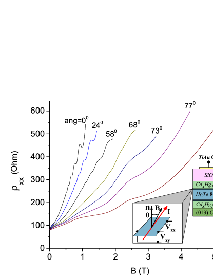
Figure 1: (color online) Dependence of resistivity $\displaystyle\rho_{xx}$ of 2D helical electrons on magnetic field, $\displaystyle B$, applied at different angles $\displaystyle\theta$ with respect to HgTe layers as labeled. Visible at $\displaystyle\theta$=0⁰ oscillating content disappears at $\displaystyle\theta>$ 73⁰. The insert shows the studied structures and geometry of the experiments. Sample TI5. $\displaystyle V_{g}$=2.5V. T=4.2K.

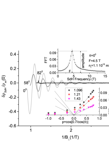
Figure 2: (color online) Dependence of normalized resistance oscillations $\displaystyle\delta\rho_{SdH}/\rho_{xx}(0)$ of 2D helical electrons on reciprocal perpendicular magnetic field, $\displaystyle B_{\perp}^{-1}$, at different angles $\displaystyle\theta$ as labeled. The amplitude of the SdH oscillations reduces with the angle and is zero at $\displaystyle\theta$=82⁰. Upper insert shows FFT spectrum of the oscillations started at $\displaystyle(B_{\perp}^{-1})^{L}$=1.09(1/T) at $\displaystyle\theta$=0⁰. Lower insert shows an angular dependence of FFT amplitude indicating significant disagreement with the one expected for ordinary degenerate 2D electrons and shown by solid straight lines. Sample TI5. $\displaystyle V_{g}$=2.5V. T=4.2K.

Studied, 80 nm wide, strained HgTe films are grown by molecular beam epitaxy on (0,1,3) CdTe substrate. Since HgTe films grown directly on CdTe suffer from dislocations due to the lattice mismatch, our 80 nm thick HgTe films were separated from the CdTe substrate by a 20 nm thin Cd_0.7Hg_0.3Te buffer layer. This buffer layer significantly increases the electron mobility up to 40 m²/(Vs).¹³ In Fig.1 the insert shows the studied structures. The 2D helical electrons are formed at the top and the bottom surfaces of the HgTe film. The structures are equipped with a TiAu gate providing the possibility to tune the Fermi energy $\displaystyle E_{F}$ inside the insulating gap $\displaystyle\Delta_{g}\approx$15 mV^{13; 20} and to change the density $\displaystyle n=n_{t}+n_{b}$ of 2D helical electrons, where $\displaystyle n_{t}$ ($\displaystyle n_{b}$) is the density of 2D electrons located at the top (bottom) of HgTe film. Magnetotransport experiments indicate that at a positive gate voltage $\displaystyle V_{g}$, $\displaystyle n_{t}>n_{b}$ since the top HgTe surface is closer to the gate.¹³

Samples are etched in the shape of a Hall bar with width $\displaystyle W=50\mu$m. Two samples are studied in magnetic fields up to 8 Tesla applied at different angle $\displaystyle\theta$ relative to the normal $\displaystyle{\bf n}$ to 2D layers and perpendicular to the applied current. The angle $\displaystyle\theta$ is evaluated using Hall resistance $\displaystyle R_{xy}$, which is proportional to the perpendicular component, $\displaystyle B_{\perp}=Bcos(\theta)$, of the total magnetic field $\displaystyle B$. Experiments indicate that 2D helical electrons located at the top of HgTe film provide the dominant contribution to SdH oscillations at small magnetic fields.^{13; 15} The density $\displaystyle n_{t}$ is estimated from the frequency of SdH oscillations taken at $\displaystyle\theta$=0⁰ (see upper insert to Fig.2). An averaged mobility obtained from Hall resistance and the resistivity at zero magnetic field for sample TI1 (TI5) is $\displaystyle\mu$=43 m²/Vs (37m²/Vs). Sample resistance was measured using the four-point probe method. We applied a 133 Hz $\displaystyle ac$ excitation $\displaystyle I_{ac}$=0.5$\displaystyle\mu$A through the current contacts and measured the longitudinal (in the direction of the electric current, $\displaystyle x$-direction) and Hall (along $\displaystyle y$-direction) voltages. The measurements were done in the linear regime in which the voltages are proportional to the applied current.

Figure 1 shows the dissipative magnetoresistivity $\displaystyle\rho_{xx}(B)$ taken at different angles $\displaystyle\theta$ as labeled. Quantum resistance oscillations are visible at $\displaystyle\theta$=0⁰, 24⁰ and 58⁰ and are significantly suppressed at $\displaystyle\theta>$68⁰. To facilitate an analysis of the oscillating content, the monotonic background, obtained by an adjacent point averaging over the period of the oscillations in reciprocal magnetic fields, is removed from the magnetoresistivity $\displaystyle\rho_{xx}(B)$. Figure 2 presents the remaining oscillating content of the magnetoresistivity, $\displaystyle\delta\rho_{SdH}$, normalized by $\displaystyle\rho_{xx}(B=0)$ as a function of the reciprocal perpendicular magnetic field $\displaystyle B_{\perp}^{-1}$.²¹ As expected, the SdH oscillations are periodic in $\displaystyle B_{\perp}^{-1}$.^{22; 19} In agreement with Fig.1, SdH oscillations decrease with the angle $\displaystyle\theta$ and are absent at $\displaystyle\theta$=82⁰. The upper insert shows the Fourier spectrum obtained by Fast Fourier Transformation (FFT) of the oscillations between $\displaystyle 1/B_{\perp}^{L}$=1.09 (1/T) and $\displaystyle 1/B_{\perp}^{R}$=5 (1/T) at $\displaystyle\theta$=0⁰.²³ The SdH frequency $\displaystyle F$=4.5(T) yields the 2D electron density $\displaystyle n_{t}=(e/h)F$=1.1 10¹⁵ m^-2.^{22; 19} The density $\displaystyle n_{t}$ stays the same at different angles $\displaystyle\theta$. A comparison with the Hall coefficient indicates a presence of a second group of 2D electrons with a density $\displaystyle n_{b}$=0.7 10¹⁵ m^-2, which should oscillate at frequency 2.9(T). These oscillations are absent in the spectrum at small $\displaystyle B_{\perp}$, which is consistent with previous experiments.¹³

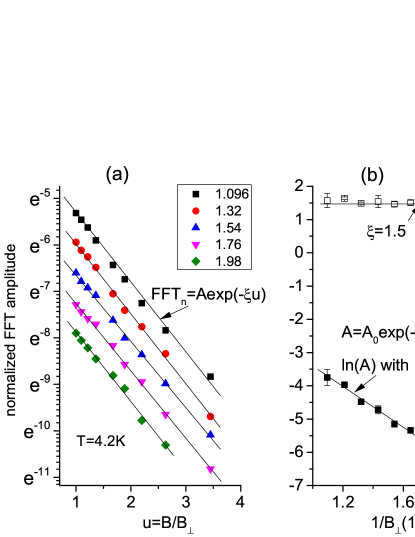
Figure 3: (color online) (a) Dependence of normalized FFT amplitude on $\displaystyle B/B_{\perp}$. FFT amplitude is obtained for SdH oscillations in interval [$\displaystyle B^{-1}_{\perp}$,5] T^-1. Symbols correspond to different $\displaystyle B^{-1}_{\perp}$ as labeled. The dependence is fitted in accordance with Eq.(1). (b) Dependence of parameters $\displaystyle\xi$ and A extracted from the fit on $\displaystyle B^{-1}_{\perp}$. The parameter $\displaystyle\xi$=1.5$\displaystyle\pm$0.15 indicates uniform ($\displaystyle B_{\perp}$-independent) relative decrease of SdH amplitude with angle $\displaystyle\theta$. Sample TI5. $\displaystyle V_{g}$=2.5V. T=4.2K.

The lower insert shows a comparison of the angular dependence of FFT amplitude with the one expected for spin degenerate 2D electron states and shown by the straight solid lines. The Zeeman effect splits the spin degenerate electron quantum levels leading to a variation of the SdH amplitude with the angle^{18; 24}: $\displaystyle A\sim p=\cos(\pi\Delta_{Z}/\Delta_{c})=\cos(\gamma/\cos(\theta))$ since the cyclotron energy $\displaystyle\Delta_{c}\sim B_{\perp}$ and the Zeeman energy $\displaystyle\Delta_{Z}\sim B$. The fitting parameter $\displaystyle\gamma=\pi gm_{c}/m_{0}$=0.7, where $\displaystyle g$ is electron g-factor and $\displaystyle m_{0}$ is free electron mass, is chosen to provide the best fit with the experiment. The comparison yields g-factor $\displaystyle g\approx$12 at cyclotron mass $\displaystyle m_{c}\approx$0.02$\displaystyle m_{0}$ determined from temperature experiments presented below. The discrepancy between the experiment and the behavior of the spin degenerate 2D electrons is seen at $\displaystyle p<$0.4, when the experimental data deviates from the straight lines. At $\displaystyle p<$0, the SdH amplitude continues to decrease in contrast to the spin degenerate case.

To analyze the observed decrease of the amplitude of SdH oscillations in a spin non-degenerate electron system, such as 2D helical electrons in the strained HgTe films,^{5; 12; 13; 14; 15; 16} one should assume that some physical parameters, controlling the SdH amplitude in Lifshits-Kosevich formula^{22; 19}, change with the magnetic field. The following relations of the quantum mean free path $\displaystyle l_{q}$ and Fermi velocity $\displaystyle v_{F}$ with the magnetic field B: $\displaystyle l_{q}^{-1}=l_{0}^{-1}(1+\alpha B)$ and $\displaystyle v_{F}^{-1}=v_{0}^{-1}(1+\beta B)$, where $\displaystyle l_{0},v_{0},\alpha,\beta$ are constants, reproduce the observed results. A substitution of these relations into Lifshits-Kosevich formula at small magnetic fields^{19; 24} yields a normalized FFT amplitude²⁵:

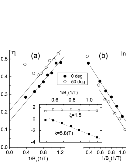
Figure 4: (a) Dependence of parameter $\displaystyle\eta=\beta au+a/B_{\perp}$ on $\displaystyle B^{-1}_{\perp}$. The parameter is extracted from FFT_n(T,u=const) set obtained at different temperatures T in the interval 5.5 to 12.5 K at a fixed angle similar to the parameter $\displaystyle\xi$ extracted from the FFT_n(u,T=const) set obtained at fixed temperature and shown in Fig.3; (b) Dependence of amplitude $\displaystyle A_{T}$ on $\displaystyle B^{-1}_{\perp}$. Different symbols correspond to different angles $\displaystyle\theta$ as labeled. Insert shows result of the rotation experiment at fixed temperature T=5.5K for the same sample. Sample TI1. $\displaystyle V_{g}$=1.7V. $\displaystyle n_{t}$=1.2 10¹⁵ m^-2.

$$FFT_{n}(u,T,B_{\perp})=A_{0}\exp(-\xi u)\exp(-\frac{k}{B_{\perp}})$$ (1)

Here $\displaystyle\xi=\alpha d+\beta aT$, $\displaystyle k=d+aT$, $\displaystyle d=\pi\hbar k_{F}/(el_{0})$, $\displaystyle a=2\pi^{2}k_{B}k_{F}/(ev_{0})$, $\displaystyle u$=$\displaystyle B/B_{\perp}$=$\displaystyle 1/\cos(\theta)$, $\displaystyle k_{F}$ is the electron wave number at $\displaystyle E_{F}$, $\displaystyle k_{B}$ is Boltzmann constant, $\displaystyle e$ is electron charge and $\displaystyle A_{0}$ is a constant. Parameters $\displaystyle d$ and $\displaystyle a$ are coming from the Dingle and temperature damping factors of the SdH amplitude.^{19; 24} A relation $\displaystyle\omega_{c}=ev_{F}B_{\perp}/(\hbar k_{F})$ is used for the cyclotron frequency.

Figure 3(a) shows a dependence of the normalized amplitude FFT_n on $\displaystyle u=B/B_{\perp}$ at different $\displaystyle B_{\perp}$ as labeled. In a broad range of $\displaystyle B_{\perp}$, the SdH amplitude decreases exponentially with $\displaystyle u$. Figure 3(b) shows that the parameter $\displaystyle\xi$ is nearly independent on $\displaystyle B_{\perp}$, while the SdH magnitude $\displaystyle A$ drops exponentially with $\displaystyle 1/B_{\perp}$. Similar results are obtained at different densities $\displaystyle n_{t}$ on both samples.

Measurements at different temperatures indicate presence of a temperature dependent contribution to $\displaystyle\xi$.²⁶ Figure 4(a) shows a dependence of the parameter $\displaystyle\eta=\beta au+a/B_{\perp}$ on $\displaystyle 1/B_{\perp}$. This parameter controls the exponential temperature variations of FFT_n in Eq.(1). The presented parameter $\displaystyle\eta$ is obtained from the T dependence of FFT_n(T,u=const) similar to the parameter $\displaystyle\xi$ found from FFT_n(u,T=const) shown in Fig.3. Fig.4(a) demonstrates that the parameter $\displaystyle\eta$ decreases linearly with decreasing $\displaystyle 1/B_{\perp}$ as expected¹⁹ yielding $\displaystyle a$=0.28$\displaystyle\pm$0.03(T/K) and the velocity $\displaystyle v_{0}$= 7.5($\displaystyle\pm 0.8$)10⁵m/s. However, in contrast to the ordinary 2D electrons, the parameter $\displaystyle\eta$ does not extrapolate to zero at $\displaystyle 1/B_{\perp}$$\displaystyle\rightarrow$0, indicating a non-zero term $\displaystyle\eta_{0}=\beta au$=0.15$\displaystyle\pm 0.03$, yielding $\displaystyle\beta$=0.5$\displaystyle\pm$0.15 at u=1 ($\displaystyle\theta$=0⁰). Taken at different angle $\displaystyle\theta$=50⁰ measurements show a consistent increase of the $\displaystyle\eta_{0}$ with the angle: $\displaystyle\eta_{0}(u=1.54)$=0.21$\displaystyle\pm$0.03.²⁷

Figure 4(b) presents a behavior of FFT amplitude $\displaystyle A_{T}=\exp[-(\alpha du+d/B_{\perp})]$ obtained from the same T-dependence of FFT_n(T,u=const) (similar to A in Fig.3(b)). The slope of the linear dependence $\displaystyle\ln(A_{T})$ vs. $\displaystyle 1/B_{\perp}$ yields $\displaystyle d$=3.5$\displaystyle\pm 0.3$. Thus at density $\displaystyle n_{t}$=1.2 10¹⁵ m^-2 the quantum mean free path is $\displaystyle l_{0}$=73 nm in the studied sample. At $\displaystyle\theta$=50⁰(u=1.54), the dependence shifts down yielding $\displaystyle\xi_{1}$=$\displaystyle\alpha d$=0.76$\displaystyle\pm$0.15 and $\displaystyle\alpha$=0.22$\displaystyle\pm$0.05. Using the obtained parameters $\displaystyle a,d,\alpha,\beta$ we evaluate the parameters $\displaystyle\xi_{ev}$=1.58$\displaystyle\pm$0.35 and $\displaystyle k_{ev}$=5$\displaystyle\pm$0.8. The estimated parameters are close to the ones obtained in the rotation experiments: $\displaystyle\xi$=1.5$\displaystyle\pm$0.1 and $\displaystyle k$=5.8$\displaystyle\pm$0.3, and shown in the insert to Fig.4. Thus, the cross examination indicates a consistency of the obtained results. A similar outcome is found at different electron density $\displaystyle n_{t}$=1.6 10¹⁵ m^-2 (not shown).

Figure 5: (a) counted from $\displaystyle C$ energy dispersion $\displaystyle\epsilon({\bf k})$ of 2D helical electrons at different values of Zeeman energy $\displaystyle\Delta$ as labeled; (b) variations of reciprocal Fermi velocity with Zeeman energy; (c) variations of normalized probability $\displaystyle P$ of electron backscattering with Zeeman energy. $\displaystyle k_{F}$=2. All parameters are in relative units.

Fig.3 and Fig.4 show good agreement between the experiements and Eq.(1) revealing unexpected and strong suppression of SdH oscillations of 2D helical electrons with the magnetic field $\displaystyle B$. At a fixed $\displaystyle B_{\perp}$ the amplitude of SdH oscillations decreases exponentially with $\displaystyle B$: $\displaystyle A_{SdH}\sim\exp[-(\xi/B_{\perp})B]$ indicating possible relevance of a spin effect, which is proportional to $\displaystyle B$.

In response to the Lorentz force, $\displaystyle{\bf F}_{L}=e{\bf v}\times{\bf B}$, electrons in a single band move in accordance with the quasi-classical theory, considering effects of the Lorentz force on the band structure to be negligibly small.³⁰ In the systems with no spin-orbit interaction the $\displaystyle{\bf k}$-space and spin $\displaystyle{\bf s}$-space are disentangled. A change of the electron energy via Zeeman effect repopulates the spin-up and spin-down subbands in the $\displaystyle{\bf k}$-space keeping the energy dispersion of electrons intact: $\displaystyle\epsilon_{\uparrow}({\bf k})$=$\displaystyle\epsilon_{\downarrow}({\bf k})$. Thus at a fixed $\displaystyle k_{F}$ (electron density) both the Lorentz force and Zeeman effect should not change the Fermi velocity $\displaystyle v_{F}$. In systems with a spin-orbit coupling a variation in the $\displaystyle{\bf s}$-space via the Zeeman term, may change the electron dispersion in the $\displaystyle{\bf k}$-space and lead to a variation of the electron velocity $\displaystyle v_{F}$. To illustrate this effect we consider a simple model of 2D helical electrons affected by the Zeeman term $\displaystyle\Delta\sim{\bf B}=(0,0,B_{z})$ . The following Hamiltonian describes 2D helical states of a 3D topological insulator (see Eq.(34) in Ref.[9])²⁸:

$$H=C+A(\sigma^{x}k_{y}-\sigma^{y}k_{x})+\Delta\sigma^{z}$$ (2)

where C and A material constants, $\displaystyle\sigma^{x,y,z}$ are Pauli matrices and $\displaystyle{\bf k}=(k_{x},k_{y})$ in the 2D electron wave vector. The Zeeman term $\displaystyle\Delta\sigma^{z}$ changes the electron spectrum leading to a spectral gap:

$$\epsilon(k)=C\pm(\Delta^{2}+A^{2}k^{2})^{1/2}$$ (3)

Fig.5(a) presents the electron spectrum at different strengths of the Zeeman term as labeled. The vertical thin line indicates the electron wave number $\displaystyle k_{F}$ at Fermi energy. Fig.5(b) shows the increase of the reciprocal Fermi velocity $\displaystyle v_{F}^{-1}=(\partial\epsilon/\partial k)^{-1}$($\displaystyle k$=$\displaystyle k_{F}$) with $\displaystyle\Delta$, following from Eq.(3). The increase is proportional to $\displaystyle B$ at a large $\displaystyle\Delta$. The model also shows an increase of the electron scattering in magnetic fields. By polarizing electron spins in the $\displaystyle z$-direction the magnetic field increases the spin overlap between incident $\displaystyle{\bf k}_{F}(\theta_{in})$ and scattered $\displaystyle{\bf k}_{F}(\theta_{fin})$ electron states. Fig.5(c) presents the dependence of a normalized rate of the electron backscattering ($\displaystyle\theta_{fin}-\theta_{in}=\pi)$ on the Zeeman term $\displaystyle\Delta\sim B$.²⁹ At $\displaystyle\Delta=0$ the rate is zero indicating the topological protection of the backscattering. With increasing $\displaystyle\Delta$ the rate increases imitating a linear dependence on $\displaystyle\Delta$ in the interval from 0.5 to 2. At high $\displaystyle\Delta$ the rate approaches 1 indicating that at high magnetic fields there are no spin restrictions on the impurity scattering since all electron spins are polarized along $\displaystyle{\bf B}$.

Despite the similarity with the experiment the model is not directly applicable to the presented data. The studied 2D helical electrons are a result of a linear superposition of electron states from several subbands and additional terms may affect the spectrum.³¹ Further investigations are required to explain the presented findings quantitatively and reveal the dominant mechanism (s) leading to the anomalous angular decay of quantum resistance oscillations of 2D helical electrons.

In summary, the angular dependence of quantum resistance oscillations of 2D helical electrons in 3D topological insulators based on strained HgTe films demonstrates exponentially strong reduction of the oscillation amplitude $\displaystyle A$ with the magnetic field $\displaystyle B$: $\displaystyle A\sim\exp[-(\xi/B_{\perp})B]$. The temperature dependence of the amplitude $\displaystyle A$ exhibits two terms contributing to the parameter $\displaystyle\xi$: $\displaystyle\xi=\xi_{1}+\xi_{2}T$. The temperature independent term, $\displaystyle\xi_{1}$ indicates considerable reduction of the quantum mean free path $\displaystyle l_{q}$ in the magnetic field $\displaystyle B$. The reduction is consistent with the form: $\displaystyle[\delta(l_{q}^{-1})]/l_{0}^{-1}$=$\displaystyle\alpha B$, where $\displaystyle\alpha$=0.22$\displaystyle\pm$0.03(T^-1) at electron density $\displaystyle n_{t}$=1.2 10¹⁵ m^-2. The $\displaystyle l_{q}$ decrease is related to the suppression of the topological protection of the helical electron states against the impurity scattering in magnetic fields. The temperature dependent term, $\displaystyle\xi_{2}T$, indicates significant increase of the reciprocal velocity $\displaystyle v_{F}^{-1}$ of 2D helical electrons in the magnetic field, which is consistent with the form: $\displaystyle[\delta v_{F}^{-1}]/v_{0}^{-1}=\beta B$, where $\displaystyle\beta$=0.5$\displaystyle\pm$0.15(T^-1) at $\displaystyle n_{t}$=1.2 10¹⁵ m^-2. This increase suggests that the magnetic field considerably modifies the dynamics of 2D helical electrons.

S. V. thanks Prof. I. Aleiner for useful discussion.This work was supported by the National Science Foundation (Division of Material Research -1702594). Novosibirsk team is supported by Russian Science Foundation (Grant No. 16-12-10041).

References

- (1) C. L. Kane and E. J. Mele, Phys.Rev.Lett. 95, 146802 (2005).
- (2) C. L. Kane and E. J. Mele, Phys. Rev. Lett. 95, 226801 (2005).
- (3) B. A. Bernevig and S. -C. Zhang, Phys. Rev. Lett. 96, 106802 (2006).
- (4) B. A. Bernevig, T. L. Hughes, and S.-C. Zhang, Science 314, 1757 (2006).
- (5) Liang Fu and C. L. Kane, Phys. Rev. B 76, 045302 (2007).
- (6) L. Fu, C. L. Kane, and E. J. Mele, Phys. Rev. Lett. 98, 106803 (2007).
- (7) D. Hsieh, D. Qian, L. Wray, Y. Xia, Y. S. Hor, R. J. Cava, and M. Z. Hasan, Nature (London) 452, 970 (2008).
- (8) M. Z. Hasan and C. L. Kane, Rev. Mod. Phys. 82, 3045 (2010).
- (9) X. -L. Qi and S.-C. Zhang, Rev. Mod. Phys. 83, 1057 (2011).
- (10) Y. Ando, J. Phys. Soc. Jpn. 82, 102001 (2013).
- (11) J. E. Moore, Nature (London) 464, 194 (2010).
- (12) C. Brune, C.X. Liu, E.G. Novik, E.M. Hankiewicz, H. Buhmann, Y.L. Chen, X.L. Qi, Z.X. Shen, S.C. Zhang, and L.W. Molenkamp, Phys. Rev. Lett. 106, 126803 (2011).
- (13) D. A. Kozlov, Z. D. Kvon, E. B. Olshanetsky, N. N. Mikhailov, S. A. Dvoretsky, and D. Weiss, Phys. Rev. Lett. 112, 196801 (2014).
- (14) C. Brune, C. Thienel, M. Stuiber, J. Bottcher, H. Buhmann, E. G. Novik, C.-X. Liu, E. M. Hankiewicz, and L.W. Molenkamp, Phys. Rev. X 4, 041045 (2014).
- (15) D. A. Kozlov, D. Bauer, J. Ziegler, R. Fischer, M. L. Savchenko, Z. D. Kvon, N. N. Mikhailov, S. A. Dvoretsky, and D. Weiss, Phys. Rev. Lett. 116, 166802 (2016).
- (16) Hubert Maier, Johannes Ziegler, Ralf Fischer, Dmitriy Kozlov, Ze Don Kvon, Nikolay Mikhailov,Sergey A. Dvoretsky and Dieter Weiss, Nature Comm. 8, 2023, (2017)
- (17) A. A. Taskin, Satoshi Sasaki, Kouji Segawa, and Yoichi Ando, Phys. Rev. Lett. 109, 066803 (2012).
- (18) F. F. Fang, and P. J. Stiles, Phys. Rev. 174, 823 (1968).
- (19) T. Ando, A. B. Fowler, and F. Stern, Rev. of Mod. Phys. B 54, 437 (1982).
- (20) Reported in this paper measurements are done, when Fermi energy is inside the gap .
- (21) The presented data are obtained when . In this regime and the amplitude of quantum oscillations in the resistivity is proportional to the one in the conductivity with an accuracy better than 3 percent in the experiemts. Here is Drude conductivity.
- (22) D. Shoenberg Magnetic oscillations in metals, (Cambridge University Press, New York, 1984).
- (23) FFT analysis enhances the separation of the SdH oscillations of 2D electrons located at the top surface from the SdH response of the bottom conducting surface oscillating at a different frequency.
- (24) William Mayer, Areg Ghazaryan, Pouyan Ghaemi, Sergey Vitkalov A. A. Bykov, Phys. Rev. B 94, 195312 (2016).
- (25) , where the factor . In practice the polynomial factor uses parameters obtained self-consistently with the exponential fits shown in Fig.(4) via several iterations.
- (26) Estimations indicate that contributions of the inelastic processes (such as electron-electron , electron-phonon scattering) to the observed temperature dependence of parameter are small. These processes are ignored in the paper.
- (27) In Fig.4(a) deviations from the straight lines at 0.5 T-1 are related to an interference between SdH oscillations of 2D electrons located at the top and bottom surfaces of HgTe film. Contributions from the bottom 2D layer oscillate at frequency 3 T and are visible in the FFT spectrum at small in agreement with the previous study.13
- (28) Liu, C.-X., X.-L. Qi, H. Zhang, X. Dai, Z. Fang, and S.-C. Zhang, Phys. Rev. B 82, 045122 (2010).
- (29) The presented probability is a square of the magnitude of the scalar product of two eigenvectors of Hamiltonian (2) corresponding to incident and scattered electron states.
- (30) J. M. Ziman Principles of the theory of solids, (Cambridge at the University Press, 1972).
- (31) O. E. Raichev, Phys. Rev. B 85, 045310 (2012).