Shear viscosity of pseudo hard-spheres

Abstract

We present molecular dynamics simulations of pseudo hard sphere fluid (generalized WCA potential with exponents (50, 49) proposed by Jover et al. J. Chem. Phys 137, (2012)) using GROMACS package. The equation of state and radial distribution functions at contact are obtained from simulations and compared to the available theory of true hard spheres (HS) and available data on pseudo hard spheres. The comparison shows agreements with data by Jover et al. and the Carnahan-Starling equation of HS. The shear viscosity is obtained from the simulations and compared to the Enskog expression and previous HS simulations. It is demonstrated that the PHS potential reproduces the HS shear viscosity accurately.

I Introduction

Hard Sphere (HS) models have been widely used as a basic approximation of a spherical atom or molecule (See, for example  pippo ), because of the simplicity of the interaction potential and the instantaneous elastic collision dynamics. Although the HS model is an idealized model, it still captures the essential physics of macroscopic behavior of real fluids, both in and out of equilibrium. Consequenly, HS-based models are often used to study and understand the thermodynamics and transport properties of liquids. Nevertheless, because HS models are highly idealised, it is difficult to make quantitative predictions for more complex molecules based on purely theoretical calculations. This is why theory based hard sphere models are often used as a basis for empirical approaches to fluid properties that go far beyond spherical molecules VW ; viscvogelmethane . This type of approach, however, requires analytical theory that can be challenging to develop, especially for more complicated models.

Because of the simple instantaneous dynamics, there are a great deal of analytical results for HS models for properties of liquids, such as equations of state carnahanstarling and transport coefficients pippo ; Chapman:52:0 . These kinds of results can still be challenging to obtain, but they provide a powerful basis for continuing development of fluid theory safths . There are also a number of extensions of HS model that still retain the instantaneous collision dynamics and therefore are still somewhat tractable when it comes to analytical approaches. Examples are sperocylinders spherocylinders , rough hard spheres Chapman:52:0 , loaded hard spheres loadedspheres , and dipolar hard spheres dhsshear ; dhsrelaxation .

In supporting this development molecular dynamics (MD) simulations are tools that have become much more commonplace, for example as numerical experiments to verify the theoretical results. Although there are available MD studies on transport coefficients of HS fluids, for example a comprehensive one by Sigurgeirsson et al.  heyes:09:0 , it is not possible to directly use the state of art simulations packages like LAMMPS, GROMACS or NAMD which provide high-speed simulations of complex and large systems Plimpton:95:0 ; Spoel:05:0 ; Phillips:05:0 . These simulation packages rely on approximately smooth dynamics, and thus do not support the HS model’s instantaneous collision dynamics.

To get around this, Jover et al. proposed a pseudo hard sphere (PHS) model which is a cut and shifted version of a Mie potential with exponents (50,49) jover:12:0 . Using this nearly hard, but smooth potential, Jover et al. have been able to reproduce structural and thermodynamic properties accurately compared with available simulation data for the original HS system. It has also been shown to provide reliable results for studying liquid-solid coexistence vega:13:0 .

The focus of the PHS research mentioned above has been primarily on equilibrium properties. However, non-equilibrium properties such as transport coefficients are much more sensitive to changes in the dynamics than equilibrium properties. Because of this, a good reproduction of equilibrium properties does not directly imply that non-equilibrium properties would be described as well. So far, only the self-diffusion was briefly tested in jover:12:0 . The performance of the PHS potential for non-equilibrium properties has therefore not been sufficiently established.

In this work, we test in detail the reliability of the (50,49) PHS potential for calculating the viscosity. We investigate the density dependence of the viscosity, and compare it to both analytical results for HS and previous MD simulations of true HS heyes:09:0 .

II Simulation setup

The Mie ($\lambda_{r},\lambda_{a}$) potential (the generalized Lennard-Jones) can be changed to a repulsive potential by shifting it by its well-depth value and equating the larger distances interactions to zero. WCA potential is one of this cut-and-shift potential which has the form

$$U_{WCA}(r)=\begin{cases}4\epsilon\big{[}\big{(}\frac{\sigma}{r}\big{)}^{12}-\big{(}\frac{\sigma}{r}\big{)}^{6}\big{]}+\epsilon;\hskip 56.9055ptr<2^{1/6}\sigma\\ \hskip 99.58464pt0;\hskip 56.9055ptr\geq 2^{1/6}\sigma\end{cases}.$$

(1)

The WCA potential can be used to present a HS system in an approximate manner. However, the reliability of the approximation depends on ($\lambda_{r},\lambda_{a}$) and on the temperature of the system. Jover et al. jover:12:0 have studied the effect of exponents $\lambda_{r}$ and $\lambda_{a}$ on the steepness and the shape of the potential. They have chosen the pair (50,49) as a compromise between fidelity of the representation of the HS and the size of the time step in MD simulations. The steeper the potential the greater the fidelity, but the smaller the time step that is required. The PHS potential proposed by Jover et al. jover:12:0 has the following form

$$U_{50,49}(r)=\begin{cases}50~{}(\frac{50}{49})^{49}\epsilon\big{[}\big{(}\frac{\sigma}{r}\big{)}^{50}-\big{(}\frac{\sigma}{r}\big{)}^{49}\big{]}+\epsilon;\hskip 56.9055ptr<\frac{50}{49}\sigma\\ \hskip 142.26378pt0;\hskip 56.9055ptr\geq\frac{50}{49}\sigma\end{cases}.$$

(2)

In addition the effect of temperature on $U_{50,49}(r)$ potential is studied in ref. jover:12:0 and is concluded that at a reduced temperature of $T^{*}=\frac{\epsilon}{k_{B}T}=2/3$ the potential produces better agreement with the true HS. They have examined this in terms of thermodynamics and structural properties.

In order to simulate the PHS model, we have used GROMACS version 5. The potential is implemented as a tabular form. The first goal was to obtain the equation of state (pressure versus density). We have simulated a box of $N=1000$ particles with LJ parameters $\sigma$, $\epsilon$ at different pressures corresponding to different densities, at reduced temperature $T^{*}=2/3$. We limit ourselves to this temperature because according to Refs. vega:13:0 ; jover:12:0 the equilibrium properties of the PHS and HS models are similar at this temperature. In what follows, all quantities are given in reduced units: $t^{*}=t\sqrt{\frac{k_{B}T}{\sigma^{2}m}}$, $r^{*}=\frac{r}{\sigma}$, $\rho^{*}=\rho\sigma^{3}$ and $P^{*}=\frac{P\sigma^{3}}{k_{B}T}$, $\eta^{*}=\eta(\frac{\sigma^{2}}{\sqrt{mk_{B}T}})$, where $\rho$, $P$ and $\eta$ denote the number density, the pressure, and the viscosity respectively. The equilibrated systems are simulated in NPT ensemble for $t^{*}=20000$ with time-step of $\delta t^{*}=0.0011$ using a Parrinello-Rahman barostat and a velocity-rescale thermostat.

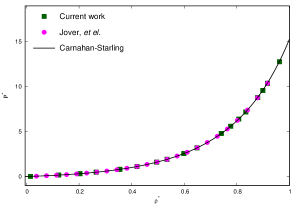
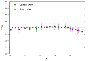
Figure 1: (Left) Reduced pressure versus reduced number density from MD simulation of PHS in this work (squares) is compared to earlier work by Jover et al.  jover:12:0 (circles) and theoretical Carnahan-Starling equation of state (solid line). (Right) The same as left plot, but rescaled with the Carnahan-Starling pressure, in order to enhance details. The errors in the current work data of $P^{*}$ are less than 4%, so are not well visible.

Simulation results for the equation of state are shown in Fig. 1. The relative errors in the pressure $P^{*}$ are less than 4%. The results agree with the results by Jover et al. jover:12:0 . They are also in good agreement with the Carnahan-Starling equation of state (solid line) Carnahan:69:00

$$P^{*}=(6/\pi)\frac{\xi(1+\xi^{*}+\xi^{*2}-\xi^{*3})}{(1-\xi^{*})^{3}},$$ (3)

$$\xi^{*}=(\pi/6)\rho^{*}.\hskip 42.67912pt$$ (4)

Ref. vega:13:0 also reports similar results using GROMACS package.

II.1 Shear viscosity

The shear viscosity can be determined both by equilibrium molecular-dynamics (EMD) or non-equilibrium molecular-dynamics (NEMD) simulations. EMD methods are based on pressure or momentum fluctuations, for example the Transverse-Current Autocorrelation Function (TCAF) method or Green-kubo method. The TCAF method is the easiest to implement and has several advantages over the Green-kubo relation. The first advantage is that any non-hydrodynamic behavior is easy to identify in the TCAF. The second advantage of the TCAF method is that it provides a natural way to estimate the magnitude of finite-size effects. This can be done in a single simulation and the results extrapolated to the infinite system limit in a straightforward calculation, (see palmer:94:0 and reference therein). In NEMD methods such as periodic perturbation (PP) method, instead of measuring intrinsic fluctuations an external force is applied to the system. The magnitude of this force is chosen such that the effects are much easier to detect than the internal fluctuations zhao:08:00 ; hess:02:0 ; Gregori:12:0 ; Gaskell:74:00 .

There are many works studying shear viscosity using MD simulations, both EMD and NEMD methods zhao:08:00 ; Gaskell:74:00 ; palmer:94:0 ; plathe:02:00 ; sunda:13:00 ; Gezeltr:10:0 ; Rowley:07:0 ; Sun:08:0 ; hess:02:0 . Here we follow the work by B. Hess hess:02:0 which studies shear viscosity determination using GROMACS. We obtain shear viscosities of PHS model from two methods: TCAF and PP. We explain both methods shortly below.

II.1.1 Transverse-current autocorrelation function

Consider an incompressible liquid with an initial velocity field generated for example by equilibrium thermal fluctuations. The velocity field can be decomposed into plane waves of the form ${\mathbb{u}}(x,0,0)=u_{0}\cos(kz)$. The solution to the Navier-Stokes equation for these components is then of the form

$$u_{x}(z,t)=u_{0}e^{-t/\tau_{r}}\cos(kz);\hskip 56.9055pt\tau_{r}=\frac{\rho}{\eta k^{2}}.$$ (5)

The solution indicates that the plane waves decay exponentially with a time constant which is inversely proportional to the viscosity $\eta$. However, at microscopic level and short time scales the behavior is not purely exponential. To account for this, a phenomenological correction can be applied by incorporating a relaxation time, leading to different solution to Eq. 5 (for details see ref. hess:02:0 );

$$u_{x}(z,t)=u_{0}e^{-t/(2\tau_{m})}\big{(}\cosh(\Omega t/(2\tau_{m}))+\frac{1}{\Omega}\sinh(\Omega t/(2\tau_{m}))\big{)}\cos(kz),$$ (6)

where

$$\Omega=\sqrt{1-4\tau_{m}\frac{\eta}{\rho}k^{2}}.$$ (7)

For large $k$ equation (6) leads to a similar solution as equation (5). The viscosity from this method is given by (palmer:94:0, )

$$\eta(k)=\eta(0)(1-ak^{2})+O(k^{4}).$$ (8)

II.1.2 The periodic perturbation method

As mentioned earlier, in PP method an external force is applied to the system. The external field leads to development of a velocity field $\mathbb{u}$ throughout the system according to the Navier-Stokes equation. For a force only in the $x$ direction, the applied acceleration $a_{x}$ for a periodic system is given as

$$a_{x}(z)=\alpha\cos(kz);\hskip 56.9055ptk=\frac{2\pi}{l_{z}},$$ (9)

where, $l_{z}$ is the height of the box and $\alpha$ is the amplitude of the acceleration. With the initial value of $u_{z}(x)=0$, the resulting velocity profile has amplitude

$$\nu(1-e^{-t/\tau_{r}}),$$ (10)

where

$$\nu=\alpha\frac{\rho}{\eta k^{2}}.$$ (11)

Thus, at each time step the average velocity can be measured and viscosity can be obtained from Eq. 11. In order to obtain accurate results efficiently, the parameters of the periodic external force must be chosen carefully. If the velocity profile does not have large fluctuations, less statistics needs to be collected, and thus the simulation time is shorter. This can be achieved with a large amplitude. However, the shear rate should also not be so high that the system moves too far from equilibrium. For more details about the method and estimation of parameters see ref. hess:02:0 .

III Shear viscosity from simulations

We first discuss the TCAF method. We take the final configurations of the NPT simulations explained in previous section and simulate the system in NVT ensemble for $t^{*}=3000$ with $\delta t^{*}=0.0011$ time step. In the TCAF method the correct values of viscosity are obtained when the velocity profile is not coupled to a heat bath. Therefore, a Berendsen thermostat with a long coupling time of $t^{*}=11$ is used in order to minimize the influence of the thermostat, see details in ref. hess:02:0 . The velocity and coordinates are stored every $\delta t^{*}=0.011$. The neighbor list was updated every $\delta t^{*}=0.005$. The resulting k-dependent viscosities from the simulations are fitted to Eq. 8 to obtain the viscosities. Fig. 2 shows an example of simulation result at density $\rho^{*}=0.8$. The resulting viscosity from the fit gives $\eta^{*}=2.11\pm.043$ in reduced unit, $\eta^{*}=\eta(\frac{\sigma^{2}}{\sqrt{mk_{B}T}})$. The obtained values of $\eta^{*}$ from this method are given in Table. 1 for various pressures/densities (the last two columns), and are shown in Figure. 3 as crosses. The errors in the given viscosities from this method are obtained from block averaging over k-dependent viscosities plus uncertainty of the fittings to Eq. 8.

Figure 2: Shear viscosity of PHS obtained from simulation at $\rho^{*}=0.80$ (data). The solid line shows the fit to Eq. 8 (TCAF method). $k^{*}=k\sigma$.

For the PP method, we simulate the system in NVT ensemble for $t^{*}=3000$ with an addition of an externally imposed acceleration hess:02:0 . The coupling time of the Berendsen thermostat is set to $t^{*}=2.84$ in oder to remove the energy introduced in the system by the external force more rapidly. The optimal acceleration amplitude was estimated (see Eqs. 22, 26, 27 in ref. hess:02:0 ) to be around $\alpha^{*}=0.054$, which is big enough to develop sufficient shear, but also not so big that the system moves too far from equilibrium. One disadvantage of this method is that the obtained viscosities depend on the chosen amplitude $\alpha$ hess:02:0 , moreover, the chosen amplitude should be changed with the density in the systems. We have started the analysis at time $300$ reduced units after the start of applying the force, so that there is enough time to develop a steady shear amplitude. The obtained values of $\eta^{*}$ from this method are given in Table. 1 (the fifth and sixth columns). The errors in the viscosities are obtained from block averaging. The results are included in Figure. 3, along with the results of the TCAF methods and the MD results of the true HS model reported by Sigurgeirsson et al. heyes:09:0 . We give the simulation results for $\rho^{*}>0.1$, because when the system is dilute the mean-free-path of the particles becomes large and the simulation box should be large enough to make the collisions to occur enough. That is computationally expensive.
The results from to the TCAF method show better agreement than the PP method. The reason is that the chosen amplitude $\alpha$ has effect on the viscosity, as studied comprehensively in ref. hess:02:0 and in order to obtain more accurate estimations from this method one should try several amplitudes for each density, which is time-consuming.

$P^{*}$	error in $P^{*}$	$\rho^{*}$	error in $\rho^{*}$	$\eta^{*}$ (PP)	error in $\eta^{*}$ (PP)	$\eta^{*}$ (TCAF)	error in $\eta^{*}$ (TCAF)
0.15978	0.00069	0.12286	0.00014	0.19115	0.01286	0.15894	0.00080
0.31944	0.00182	0.20395	0.00028	0.21134	0.01275	0.20263	0.00158
0.47930	0.00284	0.26531	0.00025	0.26418	0.01572	0.24035	0.00203
0.79872	0.00378	0.35532	0.00026	0.34591	0.01497	0.30003	0.00234
1.11829	0.00517	0.42067	0.00035	0.42858	0.01868	0.37814	0.00368
1.59719	0.00750	0.49526	0.00029	0.52196	0.02760	0.48749	0.00539
1.91703	0.00988	0.53465	0.00030	0.57531	0.02666	0.58406	0.00673
2.55643	0.01294	0.59829	0.00032	0.75286	0.02338	0.72918	0.00862
3.19444	0.01563	0.64875	0.00028	0.97986	0.03616	0.91150	0.01233
4.79239	0.02033	0.74088	0.00033	1.51894	0.05567	1.46623	0.02304
5.59744	0.03030	0.77666	0.00164	1.83790	0.04855	1.71697	0.03116
6.38936	0.02893	0.80720	0.00027	2.12458	0.04511	2.11137	0.04336
7.18685	0.02710	0.83400	0.00021	2.41335	0.07214	2.32994	0.05179
8.78463	0.03660	0.87911	0.00034	3.52977	0.09911	3.36685	0.08977
9.58201	0.04701	0.89880	0.00030	4.02040	0.09138	4.02834	0.12877
10.37838	0.04053	0.91643	0.00026	4.67897	0.09505	4.62323	0.15965
12.77719	0.04276	0.96250	0.00020	7.13797	0.11703	6.86586	0.30399

Table 1: Shear viscosity obtained from the simulations from the two different methods, PP and TCAF. The given shear viscosities are dimensionless; $\eta^{*}=\eta(\frac{\sigma^{2}}{\sqrt{mk_{B}T}})$.

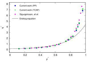
Figure 3: (Left) Shear viscosity of PHS model from TCAF method (crosses) and from PP method (squares). The red circles are results of Sigurgeirsson et al. heyes:09:0 and the solid line is the Enskog expression, Eq. 12. (Right) The same as the left plot with the Enskog equation as a base function.

IV Comparison with theory

The Enskog expression for the viscosity of a fluid of hard spheres is Chapman:52:0 ; Santos:16:0 ; Viswanath:07:0 ; Sengers:00:0 ; Lucas:79:0

$$\eta=\eta_{0}\bigg{[}g^{-1}(\sigma)+0.8~{}V_{excl}~{}\rho+0.776~{}V^{2}_{excl}~{}\rho^{2}~{}g(\sigma)\bigg{]},$$ (12)

where

$$\hskip 56.9055pt\eta_{0}=\frac{5}{16\sigma^{2}}\sqrt{\frac{mk_{B}T}{\pi}},$$ (13)

and $V_{excl}$ is the excluded volume of HS, $V_{excl}=\frac{2\pi\sigma^{3}}{3}$, and $g(\sigma)$ is the radial distribution function (rdf) at contact. $\eta_{0}$ is the zero-density viscosity. The rdf at contact can be obtained directly from the Carnahan-Starling equation of state, which yields,

$$g(\sigma)=\frac{1-\xi/2}{(1-\xi)^{3}},$$ (14)

where $\xi=\frac{\pi\rho}{6}$ is the volume fraction. It can also be found from the Percus-Yevick approximation, yelash:01:00 ; yevick:58:00 .

$$g(\sigma)=\frac{1+\xi/2}{(1-\xi)^{2}}.$$ (15)

The latter is more accurate at high density metastable fluid region heyes:09:0 .

In Figure. 3 we compare the simulation results to the Enskog theory and to the previous MD simulations of true HS simulations by Sigurgeirsson et al. heyes:09:0 . The figures present a qualitative agreement with both. Similar to the ref. heyes:09:0 the Enskog theory produces good agreements only for low- to mid-density ranges and fails at high densities, since it does not take into account correlated collisions. That is the reason for deviations at high densities in Fig. 3 Santos:16:0 ; Viswanath:07:0 ; Sengers:00:0 ; Lucas:79:0 .

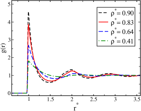
Figure 4: Radial distribution functions of PHS obtained from the simulations at several densities.

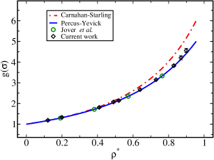
Figure 5: Radial distribution functions of PHS at contact obtained from the simulations (diamonds) along with the theoretical expressions of Carnahan-Starling (dot-dashed line) and Percus-Yevick (solid line). The circles are MD simulations by Jover et al..

We also compare the radial distribution function at contact obtained from simulations (only for several densities) to the theoretical prediction from using the Carnahan-Starling equation of state and the Percus-Yevick approximation. In order to obtain the contact values of the radial distribution functions from simulations, we first obtain the rdf profiles for each density, see Figure. 4 (the results are taken from the simulations explained in Section. II). The contact values then are collected at $r^{*}=1$. The values of the rdf at contacts are given in black diamonds in Fig. 5. Simulation results from ref. jover:12:0 are also included as circles. Eqs. 14-15 are represented in this figure by dot-dashed and solid lines, respectively. As seen in the figure, the simulation results agree well with the Percus-Yevick expression and with results produced by Jover et al. jover:12:0 . As expected Carnahan-Starling’s expression deviates at higher densities, because it does not accurately capture higher virial coefficients.

V Conclusions

We have tested the reliability of the pseudo hard sphere (PHS) potential for calculating the shear viscosity of hard spheres. We have used molecular-dynamics simulations (with GROMACS) for this purpose and obtained shear viscosities of PHS from two different methods; transverse-current autocorrelation function and the periodic perturbation method.

We have run simulations under the same conditions that have previously been confirmed to represents the hard-sphere equilibrium properties as demonstrated by Jover et al. jover:12:0 . We have compared the shear viscosities from simulations to the Enskog theory and to available MD simulation data  heyes:09:0 . Similar to  heyes:09:0 , the comparison with Enskog equation shows a good agreement for densities up to $\rho\sigma^{3}\leq 0.65$. In addition, contact values of the radial distribution functions agree with both Carnahan-Starling (at low densities) and Percus-Yevick expression (up to $\rho\sigma^{3}\approx 0.85$).

The validation of shear viscosity of PHS model helps to use it directly into the state of art simulations packages like LAMMPS, GROMACS or NAMD (which provide high-speed simulations) in order to study complex and large systems. This in turn greatly simplifies its use to support development of analytical theory for similar models based on hard spheres, such as dipolar hard spheres, which will aid the development of transport theory as well as empirical approaches to more complex liquids.

VI Acknowledgments

The work has been supported by National Infrastructure for Computational Science in Norway (UNINETT Sigma2) with computer timed for the Center for High Performance Computing (NN9573K and NN9572K). The authors acknowledge The Research Council of Norway for NFR project number 275507 and The Faculty of Engineering, Norwegian University of Science and Technology (NTNU), for financial support. FP acknowledges Prof. Erich Müller for providing data for radial distribution of PHS.

References

- (1) R. di Pippo, J. R. Dorfman, J. Kestin, H. E. Khalifa, and E. A. Mason Physica, vol. 86A, pp. 205–223, 1977.
- (2) D. D. Royal, V. Vesovic, J. P. M. Trusler, and W. A. Wakeham Mol. Phys., vol. 101, pp. 339–352, 2003.
- (3) E. Vogel, J. Wilhelm, C. Kuchenmeister, and M. Jaeschke High Temp.-High Press., vol. 32, pp. 73–81, 2000.
- (4) N. F. Carnahan and K. E. Starling J. Chem. Phys., vol. 51, p. 635, 1969.
- (5) S. Chapman and T. G. Cowling, The Mathematicaltheory of non-uniform gases. Cambridge university press, 1952.
- (6) G. Jackson and K. E. Gubbins Pure Applied Chem., vol. 61, pp. 1021–1026, 1989.
- (7) C. F. Curtiss and C. Muckenfuss, “Kinetic theory of nonspherical molecules. ii,” The Journal of Chemical Physics, vol. 26, no. 6, pp. 1619–1636, 1957.
- (8) S. I. Sandler and J. S. Dahler, “Kinetic theory of loaded spheres. ii,” The Journal of Chemical Physics, vol. 43, no. 5, pp. 1750–1759, 1965.
- (9) L. Monchick and E. A. Mason, “Transport properties of polar gases,” The Journal of Chemical Physics, vol. 35, no. 5, pp. 1676–1697, 1961.
- (10) R. D. Olmsted and C. F. Curtiss, “Transport properties of a gas of diatomic molecules. iii. rdw approximation to the rotational relaxation time,” The Journal of Chemical Physics, vol. 55, no. 7, pp. 3276–3283, 1971.
- (11) H. Sigurgeirsson and D. M. Heyes Mol. Phys, vol. 101, pp. 469–482, 2009.
- (12) S. Plimpton J. Comp. Phys., vol. 117, pp. 1–19, 1995.
- (13) D. van der Spoel, E. Lindahl, B. Hess, G. Groenhof, A. E. Mark, and H. J. Berendsen J. Comput. Chem., vol. 26, pp. 1701–1718, 2005.
- (14) J. C. Phillips, R. Braun, W. Wang, J. Gumbart, E. Tajkhorshid, E. Villa, C. Chipot, R. D. Skeel, L. Kale, and K. Schulten J. Comput. Chem., vol. 26, p. 1781, 2005.
- (15) J. Jover, A. J. Haslam, A. Galindo, G. Jackson, and E. A. Müller J. Chem. Phys, vol. 137, p. 144505, 2012.
- (16) J. R. Espinosa, E. Sanz, C. Valeriani, and C. Vega J. Chem. Phys, vol. 139, p. 144505, 2013.
- (17) N. F. Carnahan and K. E. Starling J. Chem. Phys, vol. 51, p. 635–636, 1969.
- (18) B. J. Palmer Phys. Rev. E, vol. 49, p. 1, 1994.
- (19) L. Zhao, T. Cheng, and H. Sun J. Chem. Phys, vol. 129, p. 144501, 2008.
- (20) B. Hess J. Chem. Phys, vol. 116, p. 209, 2002.
- (21) J. P. Mithen, J. Daligault, and G. Gregori Contrib. Plasma Phys., vol. 52, pp. 58–61, 2012.
- (22) T. Gaskell J. Phys. C: Solid State Phys., vol. 7, p. 1631, 1974.
- (23) P. Borat and F. müller-Plathe J. Chem. Phys, vol. 116, pp. 3362–3369, 2002.
- (24) A. P. Sunda and A. Venkatnathan Mol. Simul., vol. 39, pp. 728–733, 2013.
- (25) S. Kuang and J. D. Gezeltr J. Chem. Phys, vol. 133, p. 164101, 2010.
- (26) J. C. Thomas and R. L. Rowley J. Chem. Phys, vol. 127, p. 174510, 2007.
- (27) L. Zhao, T. Cheng, and H. Sun J. Chem. Phys, vol. 129, p. 144501, 2008.
- (28) A. Santos, A Concise Course on the Theory of Classical Liquids, Basic and Selected Topics. Springer, 2016.
- (29) D. S. Viswanath, T. K. Ghosh, D. H. L. Prasad, N. V. K. Dutt, and K. Y. Rani, Viscosity of Liquids; Theory, Estimaation, Experiment, and Data. Springer, 2007.
- (30) J. V. Sengers, R. F. Kayser, C. J. Peters, and H. J. White, Equations of State for Fluids and Fluid Mixtures. Elsevier, 2000.
- (31) K. Stephan and K. Lucas, Viscosity of Dense Fluids. Springer, 1979.
- (32) L. V. Yelash and T. Kraska vol. 3, p. 3114, 2001.
- (33) J. K. Percus and G. J. Yevick Phys. Rep, vol. 110, p. 1–13, 1958.