Impact of temporal connectivity patterns on epidemic process

Abstract

To provide a comprehensive view for dynamics of and on many real-world temporal networks, we investigate the interplay of temporal connectivity patterns and spreading phenomena, in terms of the susceptible-infected-removed (SIR) model on the modified activity-driven temporal network (ADTN) with memory. In particular, we focus on how the epidemic threshold of the SIR model is affected by the heterogeneity of nodal activities and the memory strength in temporal and static regimes, respectively. While strong ties (memory) between nodes inhibit the spread of epidemic to be localized, the heterogeneity of nodal activities enhances it to be globalized initially. Since the epidemic threshold of the SIR model is very sensitive to the degree distribution of nodes in static networks, we test the SIR model on the modified ADTNs with the possible set of the activity exponents and the memory exponents that generates the same degree distributions in temporal networks. We also discuss the role of spatiotemporal scaling properties of the largest cluster and the maximum degree in the epidemic threshold. It is observed that the presence of highly active nodes enables to trigger the initial spread of epidemic in a short period of time, but it also limits its final spread to the entire network. This implies that there is the trade-off between the spreading time of epidemic and its outbreak size. Finally, we suggest the phase diagram of the SIR model on ADTNs and the optimal condition for the spread of epidemic under the circumstances.

1 Introduction

Epidemic processes on networks have been widely used to understand the influence of network features, such as hubs and community structures, on spreading phenomena. In the past, most studies focused on static networks, where network topologies are fixed in time. However, real-world networks are highly dynamic in time, so-called temporal networks, where both nodes and links appear or disappear over time Holme2012 ; Holme2015 . The availability of high-resolution data on time-ordered interactions provides a wealth of information for the interaction patterns of nodes Cattuto2010 ; Stehle2011 ; Barrat2013 ; Fournet2014 .

Among temporal network models proposed to explain the heterogeneity of connectivity patterns, the activity-driven temporal network (ADTN) model Perra2012 , in which each node has its own activity, was successful to generate the variety of temporal networks, distinct from static ones. In the ADTN model, at each time step, nodes are activated according to pre-assigned activities, and the active nodes generate links to randomly selected nodes. Since in real networks, nodal connections are not completely random but rather the results of a non-Markovian process with memory Granovetter1973 ; Onnela2007 ; Miritello2011 ; Vestergaard2014 ; Saramaki2014 ; Rocha2016 ; Kobayashi2019 , the effect of memory was also widely considered as well as attributes: social ties, burstiness, and communities Karsai2014 ; Medus2014 ; Kim2015 ; Sun2015 ; Ubaldi2016 ; Kim2018 . Memory induces heterogeneous temporal connectivity patterns with non-trivial correlations. Based on the earlier studies of epidemic processes Rocha2011 ; Karsai2011 ; Castellano2012 ; Scholtes2014 ; Rosvall2014 ; Gleeson2016 , non-trivial connectivity patterns enable to either speed up or slow down the spread of epidemic. Such impacts of connectivity patterns were studied on a variety of temporal networks Rizzo2014 ; Liu2014 ; Tizzani2018 ; Nadini2018 ; Valdano2018 ; Moinet2018 ; Williams2018 ; Petri2018 ; Li2019 , which mostly focused on the effect of non-Markovian dynamics on the spread of epidemic, and discussed changes in outcomes.

Regarding the contrasting effects of strong ties, Sun and coworkers Sun2015 studied the role of memory in epidemic processes on ADTN models with the comparison of empirical data analyses, where memory can decrease or increase the epidemic threshold. Most recently, Tizzani and coworkers Tizzani2018 has extended the study with the elaborated memory that is tunable as the aging effect. Based on the activity-based mean-field (ABMF) approximation as well as numerical simulations, they claimed that memory are related to the reinforcement of activity-fluctuation effects. As a result, the epidemic threshold can be either decreased or increased, compared to the ABMF asymptotic value depending on the initial setup. However, there is still a lack of comprehensive understanding of the interplay between the epidemic outcomes and the topological features of ADTNs with memory.

In this paper, we investigate the role of temporal connectivity patterns in spreading phenomena as well as the optimal condition for the spread of epidemic, in terms of the susceptible-infected-recovered (SIR) model on the modified ADTN model Kim2015 with memory. In particular, we focus on how temporal connectivity patterns affect the epidemic threshold and the outbreak size in the SIR model. We find that it is crucial to consider the effective size of temporal networks, such as the spatiotemporal properties of the largest cluster size and the maximum degree. In the presence of memory, the spread of epidemic becomes slowing down and the epidemic threshold gets larger than the memoryless case. The heterogeneity of nodal activities may enhance the spread of epidemic at the initial spreading time of the epidemic, but may inhibit it later due to no reinfection. The trade-off exists between the spreading time and the outbreak size, which depends on the topological condition to reach its best prevalence.

The rest of the paper is organized as follows. In Sec. 2, we briefly describe the modified ADTN model with memory, and show time-varying network topologies. In Sec. 3, the SIR model is tested on the modified ADTN model. Based on numerical results, we propose the phase diagram of the SIR model on ADTNs. We also discuss the optimal condition to achieve both the early onset and wide prevalence of the epidemic under the circumstances. Finally, we summarize our results and provide some remarks in Sec. 4.

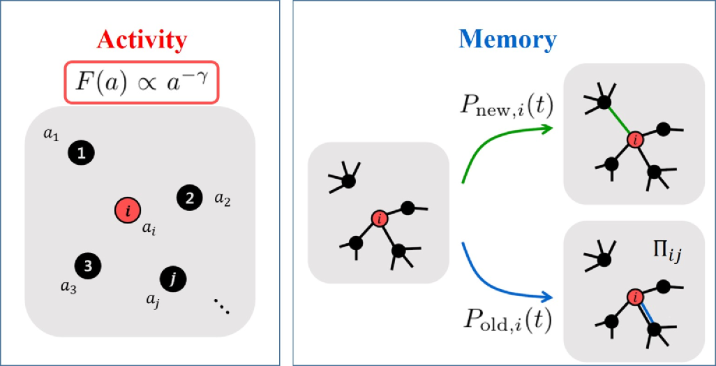
Figure 1: The modified ADTN model dynamics was illustrated as two panels: The left one represents how to activate a node, while the right one represents how for the activated node to be connected to another node. Here $F(a)$ is the distribution of nodel activitites, $P_{{\rm new(old)},i}$ is the probability that the activated node $i$ is connected to a new (old) neighbor, and $\Pi_{ij}$ is the preference probability between node $i$ and node $j$, see Eq. (1) for detailed mathematical expressions. The background links shown in the memory panel, correspond to the time-aggregated version, which are not shown at time $t$.

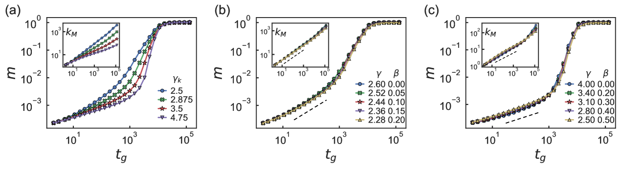
Figure 2: The fraction of the largest cluster (giant connected component, GCC), $m(t_{g})=M(t_{g})/N$, is plotted as a function of the growth time, $t_{g}$ in the modified ADTN model, where the total number of nodes is $N=10^{4}$: (a) $\beta=0,0.2,0.4,$ and $0.6$ (from top to bottom) with $\gamma=2.5$. From $\gamma_{k}=(\gamma-\beta)/(1-\beta)$, (b) $\gamma_{k}=2.60$ and (c) $\gamma_{k}=4.00$, respectively. The insets show the maximum degree, $k_{M}$, as a function of $t_{g}$. The dashed lines are guide for the eye, whose slopes represent the values of the growth exponent $\eta=1/(\gamma_{k}-1)$, so (a) $\eta=5/8$ and (b) $\eta=1/3$. Numerical data are averaged over $500$ network samples.

2 Modified ADTN model

The modified activity-driven temporal network (ADTN) model Kim2015 is a simple variant of the ADTN model Perra2012 , which allows to control the memory strength with the memory exponent $\beta$, provided that the heterogeneity of nodal activities is controlled by the activity exponent $\gamma$ in the original ADTN model. In this section, we briefly describe how to generate an ADTN with memory and discuss relevant physical properties, compared to the static case.

2.1 How to generate an ADTN with memory

We start with $N$ disconnected nodes, which have the pre-assigned own activities, $a_{i}$ ($i\in\mathcal{N}=\{1,...,N\}$) from the activity distribution $F(a)$, where $i$ is the nodal index. For the heterogeneity of nodal activities, we consider a power-law activity distribution with the activity exponent $\gamma$, so that $F(a)\sim a^{-\gamma}$.

As shown in Fig. 1, at each time step $t$, we choose node $i$ to be activated with the probability $p_{i}=a_{i}/a_{\text{max}}$, where $a_{\text{max}}=\max_{j=1}^{N}\{a_{j}\}$. The activated node $i$ can generate either a new link to a node among the nodes that have never had a link to node $i$ or an old one among the nodes that have ever had a link to node $i$ until time $t$. For the former, with probability $P_{{\rm new},i}(t)$, node $i$ connects to a randomly selected one among new nodes. For the latter, with probability $P_{{\rm old},i}(t)=1-P_{{\rm new},i}(t)$, it connects to an old node $j(\neq i)$ with the preference probability $\Pi_{ij}(t)$.

We define $P_{{\rm new},i}(t)$ and $\Pi_{ij}$ as follows:

$$P_{{\rm new},i}(t)=As_{i}(t)^{-\beta}~{}~{}\mbox{and}~{}~{}\Pi_{ij}(t)= \frac{w_{ij}(t)}{\sum_{l\in\mathcal{N}}w_{il}(t)},$$ (1)

where $\beta$, $s_{i}(t)$, and $w_{ij}(t)$ are the memory exponent from 0 (memoryless) to 1, the accumulated strength of node $i$, and the accumulated link-weight between nodes $i$ and $j$ up to time $t$, respectively. For the simplicity, we set $A=1$ without loss of generality. For the case of $\beta=0$ (memoryless), $P_{{\rm new},i}(t)$ becomes time-independent, while for the case of $\beta\neq 0$, the activated node $i$ prefers to choose an old link rather than to make a new one. Thus, the larger $\beta$, the stronger tie (the larger link-weight) between already connected nodes. In the time-accumulated network representation of the modified ADTN model with $\gamma$ and $\beta$, the generated temporal network becomes the weighted scale-free network that has the following statistics of network properties: $P(s)\sim s^{-\gamma_{s}}$ with $\gamma_{s}=\gamma$, $P(k)\sim k^{-\gamma_{k}}$ with $\gamma_{k}=\frac{(\gamma-\beta)}{(1-\beta)}$, and $P(w)\sim w^{-\gamma_{w}}$ with $\gamma_{w}=\gamma$ as $\beta\rightarrow 1$ (see the detailed derivation can be found in Ref. Kim2018 ).

2.2 Growth of largest cluster and maximum degree

The largest cluster size, $M$, and the maximum degree $k_{M}$, (i.e., the effective size of connections) are important features that compose the network properties of a ADTN. In order to reveal the effects of connectivity patterns on time-varying topologies, we revisit the growth pattern of the network structure discussed in our previous study Kim2018 for dynamic topologies as a function of sequence $t$, defined as the number of the events (links).

In Fig. 2, the main plots show the growth patterns of the fraction of the largest cluster size (giant connect component, GCC), $m=M/N$, up to the accumulated time $t_{g}$, i.e. for various $\gamma$ and $\beta$ against $t_{g}$. There are three regimes in the growth of GCC: In the dynamic regime, it grows depending on connectivity patterns of the corresponding network properties. In the intermediate-time regime, the finite-size effect comes in, and, it eventually saturates to $1$ in the static regime. Based on the dynamic scaling of the GCC in our early study Kim2018 , we readdress the growth pattern of the GCC in the dynamic regime is related to the nature of the temporal network, and plays a crucial role in network analyses. In Fig. 2 (a), we test the role of $\beta$ in the growth of the GCC at $\gamma=2.5$, which represents $\gamma_{k}=2.5~{}(\beta=0),~{}2.875~{}(0.2),3.5~{}(0.4),~{}\mbox{and}~{}4.75~{}(0.6)$. As $\beta$ (the strength of memory) increases, the GCC grows slowly because nodes prefer to contact with already connected (old) nodes. For this case, the growth pattern of the GCC depends on the degree distribution obtained from temporal connectivity patterns between nodes.

As shown in (b) and (c) of Fig. 2, the temporal growth pattern of the GCC can be categorized by the degree exponent $\gamma_{k}=(\gamma-\beta)/(1-\beta)$ among different connectivity patterns with a variety of settings with $\gamma$ and $\beta$. In the dynamic regime, the GCC exhibits the same scaling behavior as $M\sim k_{M}$, so that

$$M(t)\sim k_{M}(t)\sim t^{\eta}$$ (2)

with the natural cutoff degree scaling $\eta=1/(\gamma_{k}-1)$.

For the small values of $\gamma$, the GCC is created by a few highly active nodes, resulting in $M(t)$ growing quickly, while for the large values of $\beta$, the growth of the GCC is delayed due to the establishment of strong ties related to memory. As a result, the growth pattern of the GCC for small $\gamma$ and large $\beta$ is effectively the same as that for large $\gamma$ and small $\beta$. The growth of the maximum degree in the time-accumulated network is shown in the insets of Fig. 2, which implies that the effective size of nodal connections with different activities and memory strengths can be the same if networks have the same degree exponent.

Since temporal connectivity patterns may affect not only network topologies but also dynamic processes on them, it is interesting to discuss the effect of temporal connectivity patterns on spreading phenomena. In the next section, we revisit the susceptible-infected-recovered (SIR) model on temporal networks Sun2015 ; Tizzani2018 , in terms of ADTNs with memory, and provide a comprehensive view for the epidemic threshold in temporal networks, compared to that in static one.

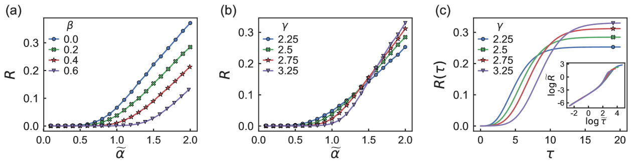
Figure 3: In the steady-state limit, the fraction of final recovered nodes (outbreak size), $R$, is plotted as a function of $\widetilde{\alpha}$: (a) the memory effect is tested on the SIR model with $\gamma=2.5$ for $\beta=0,0.2,0.4,$ and $0.6$, and (b) the role of the activity heterogeneity is tested in the SIR model with $\beta=0.2$ for $\gamma=2.25,2.5,2.75,$ and $3.25$ in the presence of memory. (c) The temporal behavior of $R$ at $\widetilde{\alpha}\approx 2.0$ of (b) is drawn against $\tau=t/N$, where the inset shows the best collapse until the first kink part of the each curve from the scaling ansatz from Eq. (4), where $\widetilde{R}=Rk_{M}$, $\widetilde{\tau}=\tau k_{M}$, and $k_{M}(t)\sim t^{\eta}$ with $\eta=1/(\gamma_{k}-1)$. Here $N=10^{4}$ and numerical data are averaged over 100 network samples with 500 samples of different initial conditions.

3 Epidemics on ADTN with memory

3.1 SIR dynamics

The modified ADTN in which an epidemic spreads can be represented as a set of time-ordered subnetworks $G_{n}$ ($n=1,2,...$). Each subnetwork $G_{n}$ represents a network accumulated during the interval $[(n-1)\Delta t,n\Delta t)$. In this paper, we set $\Delta t=10$ to investigate the effect of temporal connectivity patterns on epidemics.

We consider the classic SIR model, where a node can be one of three states: Susceptible (S) nodes are uninfected (healthy) that can be infected at a rate of $\alpha$ if they are in contact with infected neighboring nodes at time $t$. Infected (I) nodes spread the epidemic to susceptible nodes that also recover themselves at a rate of $\mu$. Then I nodes become recovered (R) ones are permanently immune that are not further involved in dynamic. In this sense, R nodes are also often called removed ones. The dynamics of the SIR model is as follows:

$${\rm\bf S}+{\rm\bf I} \xrightarrow{~{}\alpha~{}}2{\rm\bf I},$$

$$~{}{\rm\bf I} \xrightarrow{~{}\mu~{}}{\rm\bf R}.$$ (3)

In the SIR model, the initial states of all nodes are S, except for one seed I node that is selected at random. At each network step $n$, the epidemic spreads in the network $G_{n}$. Each S node in $G_{n}$ is infected with probability $p_{\alpha}$ if it contacts with an I node. At the same time, all I nodes change to R nodes with probability $p_{\mu}$. At the next network step $n+1$, the network $G_{n}$ is changed to $G_{n+1}$, and the dynamic process is repeated in $G_{n+1}$. This procedure repeats until the last subnetwork. Note that $p_{\alpha}$ is the probability per contact, so $p_{\alpha}=\alpha/\langle k\rangle$, where $\langle k\rangle$ is the average degree per unit step. Here we use $N=10^{4}$ in the modified ADTN model and $\mu=10^{-3}$ in the SIR model. Numerical data are averaged over $100$ network configurations with $500$ independent simulations of initial conditions.

3.2 Epidemic threshold and outbreak size

In the SIR model, the outbreak size and the epidemic threshold are the most interesting physical quantities. The outbreak size $R$ can be measured as the fraction of R nodes and the epidemic threshold $\widetilde{\alpha}=\alpha/\mu$ indicates the ordinary bond percolation transition Cohen2002 , which separates the epidemic phase from the infection-free phase. Below $\widetilde{\alpha}_{c}$, $R\to 0$ in the thermodynamic limit ($N\to\infty$).

In modified ADTNs as $\gamma$ and $\beta$ vary, we discuss how temporal connectivity patterns affect $R$ and $\widetilde{\alpha}_{c}$ as shown in Fig. 3 and Fig. 4. In Fig. 3, we test (a) the role of memory in the final outbreak and (b) the heterogeneity of nodal activities in the presence of memory, respectively. Moreover, we investigate temporal behaviors of (b) at $\widetilde{\alpha}\approx 2.0$ in the supercritical regime as (c), where we observe some trade-off between the spreading time and the outbreak size according to the activity exponent. Based on the detailed analysis, we find that the early-time growth of $R$ is governed by the growth of the GCC (or the maximum degree), so that we can collapse temporal data of $R$ by using the following scaling ansatz:

$$R(\tau)=k_{M}f(\tau k_{M}),$$ (4)

where $\tau$ is the rescaled time by $N$, and $k_{M}\sim t^{\eta}$ with $\eta=1/(\gamma_{k}-1)=(\gamma-1)/(1-\beta)$ in the modified ADTN model Kim2015 ; Kim2018 . The numerical confirmation is provided as the inset of (c) in Fig. 3.

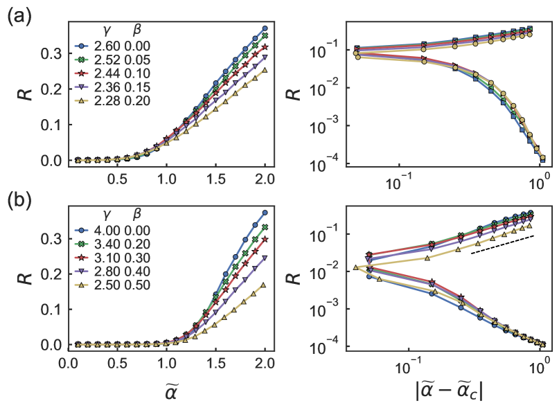
Figure 4: For the proper combinations of $\beta$ and $\gamma$ to generate the same degree exponent $\gamma_{k}$, $R$ is plotted in the left panel as the format of real scales against $\widetilde{\alpha}$ and in the right panel as the format of double-logarithmic scales against $|\widetilde{\alpha}-\widetilde{\alpha}_{c}|$, where $\widetilde{\alpha}_{c}$ depends on $\gamma_{k}$: (a) $\gamma_{k}=2.6$ and (b) $\gamma_{k}=4.0$, where $N=10^{4}$ and $\widetilde{\alpha}_{c}$ is numerically obtained. The dashed line in the right panel of (b) is guide for the eye, whose slope is $\beta_{{}_{\rm SIR}}=1/(\gamma_{k}-3)$ for $\gamma_{k}>3$.

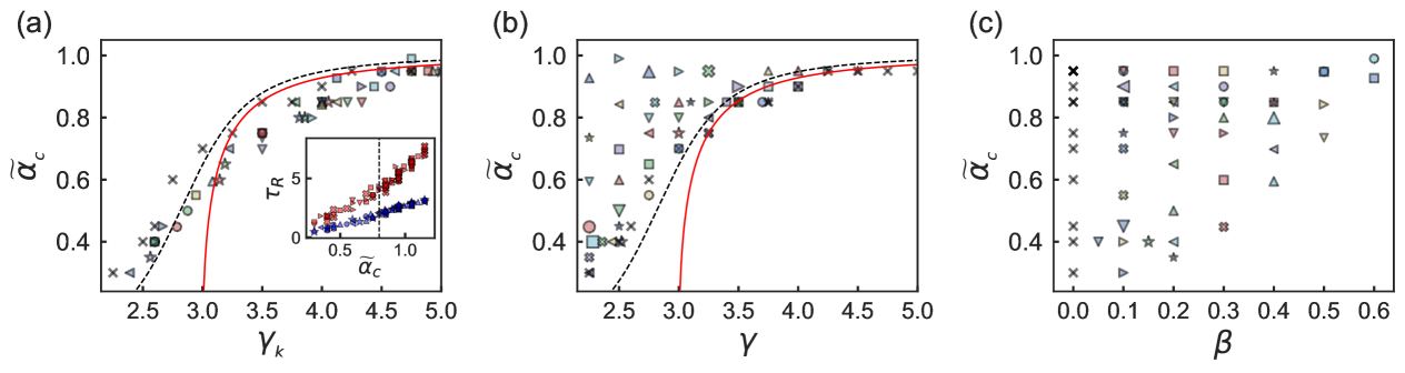
Figure 5: The phase diagram of the SIR model is drawn on the modified ADTN model: the epidemic threshold, $\widetilde{\alpha}_{c}$, is plotted against (a) the degree exponent, $\gamma_{k}$, (b) the activity exponent, $\gamma$, and (c) the memory exponent, $\beta$. In (a), the dashed (black) and solid (red) lines are guide for the eye, which are the ABMF results for $N=10^{4}$ and the thermodynamic limit, respectively (see Eq. (5) for detailed analytic expressions), the inset of which represent the plots of the rescaled access time, $\tau_{R}$, when $R=10^{-3}~{}(\mbox{bottom, blue})$ and $R=10^{-2}~{}(\mbox{top, red})$ against $\widetilde{\alpha}_{c}$ of each dataset. The values of $\tau_{R}$ are taken from the main plot of (c) in Fig. 3. The vertical dotted line of the inset in (a) corresponds to the data at $(\gamma_{k},\widetilde{\alpha}_{c})\approx(3.85,0.80)$ in the main plot. Here numerical data are averaged over 100 network samples and 500 samples of different initial conditions for $N=10^{4}$.

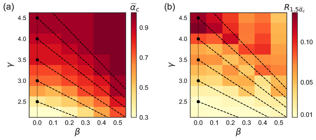
Figure 6: The optimization conditions of the epidemic threshold, $\widetilde{\alpha}_{c}$, and the outbreak size, $R_{1.5\widetilde{\alpha}_{c}}$ at $\widetilde{\alpha}=1.5\widetilde{\alpha}_{c}$, of the SIR model on ADTNs with and without memory in the plane of $\gamma$ and $\beta$: (a) the heatmap of $\widetilde{\alpha}_{c}$ and (b) that of $R_{1.5\widetilde{\alpha}_{c}}$. The dashed lines are guide for the eye, which represent the same values of $\gamma_{k}=(\gamma-\beta)/(1-\beta)$.

Based on numerical simulations, we find that $R$ and $\widetilde{\alpha}_{c}$ depend on not only temporal connectivity patterns but also network degree structures. Thus, we suggest the same analysis in static networks for the data obtained from the same degree exponent $\gamma_{k}$, consisting of different $\gamma$ and $\beta$. In Fig. 4, we test (a) $\gamma_{k}=2.60$ and (b) $\gamma_{k}=4.00$. As expected, the epidemic threshold $\widetilde{\alpha}_{c}$ is still the same even if temporal connectivity patterns are different, while the value of the outbreak size $R$ in the supercritical regime is memory-dependent. The strong the strength of memory (the larger $\beta$), the smaller the outbreak size.

To numerically estimate $\alpha_{c}$ in finite systems, we propose the criterion for the criticality in ADTNs: At the criticality of the SIR model, we assume $R_{c}=cN^{-\eta}$ from Eq. (4), where we set $c=10^{-1}$. Using the numerical estimation for the value of $\widetilde{\alpha}_{c}$ at $R=R_{c}$, we replot $R$ against $|\widetilde{\alpha}-\widetilde{\alpha}_{c}|$ in the right panels of Fig. 4 (a) and (b), respectively. The dashed line in (a) is a guide for the eye, whose slope corresponds to $\beta_{\rm{}_{SIR}}=1/(\gamma_{k}-1)$ for $\gamma_{k}>3$ from $R\sim(\widetilde{\alpha}-\widetilde{\alpha}_{c})^{\beta_{{}_{\rm SIR}}}$ in the supercritical regime.

Our numerical estimates of the epidemic threshold for various cases are shown in Fig. 5, where they are is plotted against (a) $\gamma_{k}$, (b) $\gamma$, and $\beta$, respectively. In Fig. 5 (a) and (b), we also provide the analytic curve obtained from the activity-based MF (ABMF) approximation Perra2012 ; Sun2015 ; Tizzani2018 for the memoryless case, which is as follows:

$$\widetilde{\alpha}_{c,{\rm ABMF}}=\frac{2\langle a\rangle}{\langle a\rangle+\sqrt{\langle a^{2}\rangle}},$$ (5)

where $a$ is the nodal activity.

Interestingly, we find that the epidemic threshold seems to be well described by $\gamma_{k}$. Moreover, for $\gamma<4.0$, the memory effect becomes relevant to increase the epidemic threshold, compared to that for the memoryless case, which is consistent with the result of the most recent study Tizzani2018 .

3.3 Optimal conditions for the spread of epidemic

Figure 5 (a) shows the phase diagram of the SIR model on ADTNs with memory as $\gamma_{k}$ varies. For the same $\gamma$, the epidemic threshold $\widetilde{\alpha}_{c}$ increase as $\beta$ increases, which is shown in Fig. 5 (b). For the same $\beta$, it increases as $\gamma$ increases, which is shown in Fig. 5 (c). Regarding the spreading time (speed) that is shown in the inset of Fig. 5, the smaller the epidemic threshold, the faster the spreading speed. However, it is not always guaranteed that the outbreak size is also large.

To discuss the optimal conditions for the spread of epidemic, we present the epidemic threshold and the outbreak size as the format of heatmap in the plane of the activity exponent ($\gamma$) and the memory exponent ($\beta$), see Fig. 6. As shown in Fig. 6 (a), the smaller the strength of memory ($\beta\to 0$) and the larger the activity heterogeneity ($\gamma\to 2$), the smaller the epidemic threshold ($\widetilde{\alpha}_{c}\to 0$). In the supercritical regime, $\widetilde{\alpha}>\widetilde{\alpha}_{c}$, see Fig. 6 (b), the smaller the strength of memory ($\beta\to 0$) and the larger the heterogeneity of nodal activities ($\gamma\to 4.5$), the larger the outbreak size. This is due to the trade-off between the initial spreading speed and the final outbreak size.

In other words, for both the early onset and the final prevalence, the memory effect in temporal connectivity patterns diminishes the efficiency of $\widetilde{\alpha}$. For the same $\beta$, the heterogeneity of nodal activities enhances the efficiency of $\widetilde{\alpha}$ for the early onset, but it eventually diminishes the efficiency of $\widetilde{\alpha}$ for the final prevalence. This is because highly active nodes trigger the early onset but eventually suppress the final prevalence to the entire network.

It is found that optimal conditions for the temporal spread of epidemic are sensitive to connectivity patterns. However, the epidemic threshold and the final prevalence are governed by the degree distribution that is generated by temporal connectivity patterns with the heterogeneity of nodal activities $\gamma$ and the strength of memory $\beta$. The dashed lines in Fig. 6 are drawn by the degree exponent $\gamma_{k}=(\gamma-\beta)/(1-\beta)$ of network structures.

4 Summary and remarks

To sum up, we revisited the effect of temporal connectivity patterns on epidemic process, in terms of the susceptible-infected-recovered (SIR) model on our modified activity-driven temporal networks (ADTNs) with memory, where we focused on how the epidemic threshold and the outbreaks are affected by temporal connectivity patterns with the activity heterogeneity and the strength of memory. The epidemic threshold was found to be directly related to the degree exponent of accumulated connectivity patterns in ADTNs, even though the networks were generated with different connectivity patterns. We also found that the initial spreading speed of epidemic is inversely proportional to the value of the epidemic threshold. Despite this, the case where the epidemic threshold is small cannot lead to a large outbreak size. Such behaviors are caused by memory and the activity heterogeneity in modified ADTNs. Memory that often establishes strong ties makes the spread of epidemic slow, which implies that the epidemic threshold increases and the outbreak size decreases as the strength of memory becomes stronger. The heterogeneity of nodal activities reduces the epidemic threshold, while the dominance of a few highly active nodes inhibits the propagation of epidemic to the entire network.

Based on our results, we presented the optimal strategies for the spread of epidemic in temporal networks: To successful propagate an epidemic in a short period of time, the presence of highly active nodes (in time-accumulated network representation, hubs with larger degrees), is important because it may be a good strategy to focus on a few highly active nodes and support the activation of such nodes. Otherwise, to propagate the epidemic throughout the whole network, it is better to give equal opportunities to all nodes rather than to focus on a few of active one. Ultimately, we enable to maximize the efficiency of the spread using both strategies by controlling the characteristics of temporal connectivity patterns as well as network structures according to the temporal stages of the epidemic. Therefore, the optimal conditions for each stage can be suggested by considering the trade-off between the time cost and the infection rate.

There are still important tasks remaining, such as the numerical confirmation of the activity-based mean-field approximation with memory Tizzani2018 , the finite-size scaling analysis of the SIR model with the comparison of that in static networks, and dynamic properties of connectivity patterns according to the time resolution of ADTNs, similar to Kim2018 . However, these are out of our scope in this paper since we here like to focus on the validity check for our scenario that the degree distribution determines the epidemic threshold even in ADTNs, while temporal connectivity patterns control the final prevalence and the optimal condition for the spread of epidemic. This is related to spreading phenomena that arise from the monopoly of minority groups in the real world, for example, in the development of technology and the expansion of business. Our study might highlight the importance of the balance of activities between a small number of leader groups and other groups for the early growth and overall development. As a possible future work, it would be interesting to apply our study to real-world data or to find the optimal condition in other types of connectivity patterns, such as triadic-closure connections.

Authors contribution statement

All authors designed the research and wrote the manuscript equally. Particularly, numerical simulations were performed by H.K. and analytic results with intuitive arguments were developed by M.H., and the validity check of main results were confirmed by all authors.

This research was supported by Basic Science Research Program through the National Research Foundation of Korea (NRF) (KR) [Grants No. NRF-2017R1A2B3006930 (H.K., H.J.) and NRF-2017R1D1A3A03000578 (M.H.)].

References

- (1) P. Holme and J. Saramäki, “Temporal networks,” Phys. Rep., vol. 519, no. 3, pp. 97–125, 2012.
- (2) P. Holme, “Modern temporal network theory: a colloquium,” Eur. Phys. J. B, vol. 88, no. 9, p. 234, 2015.
- (3) C. Cattuto, W. Van den Broeck, A. Barrat, V. Colizza, J.-F. Pinton, and A. Vespignani, “Dynamics of Person-to-Person Interactions from Distributed RFID Sensor Networks,” PLoS One, vol. 5, p. e11596, 07 2010.
- (4) J. Stehlé, N. Voirin, A. Barrat, C. Cattuto, L. Isella, J.-F. Pinton, M. Quaggiotto, W. Van den Broeck, C. Régis, B. Lina, and P. Vanhems, “High-Resolution Measurements of Face-to-Face Contact Patterns in a Primary School,” PLoS One, vol. 6, p. e23176, 08 2011.
- (5) A. Barrat, C. Cattuto, V. Colizza, F. Gesualdo, L. Isella, E. Pandolfi, J. F. Pinton, L. Ravà, C. Rizzo, M. Romano, J. Stehlé, A. E. Tozzi, and W. Van den Broeck, “Empirical temporal networks of face-to-face human interactions,” Eur. Phys. J. Spec. Top., vol. 222, pp. 1295–1309, Sep 2013.
- (6) J. Fournet and A. Barrat, “Contact Patterns among High School Students,” PLoS One, vol. 9, p. e107878, 09 2014.
- (7) N. Perra, B. Gonçalves, R. Pastor-Satorras, and A. Vespignani, “Activity driven modeling of time varying networks,” Sci. Rep., vol. 2, p. 469, 2012.
- (8) M. S. Granovetter, “The Strength of Weak Ties,” Am. J. Sociol., vol. 78, no. 6, pp. 1360–1380, 1973.
- (9) J.-P. Onnela, J. Saramäki, J. Hyvönen, G. Szabó, D. Lazer, K. Kaski, J. Kertész, and A.-L. Barabási, “Structure and tie strengths in mobile communication networks,” Proc. Natl. Acad. Sci. USA, vol. 104, pp. 7332–7336, 2007.
- (10) G. Miritello, E. Moro, and R. Lara, “Dynamical strength of social ties in information spreading,” Phys. Rev. E, vol. 83, p. 045102, Apr 2011.
- (11) C. L. Vestergaard, M. Génois, and A. Barrat, “How memory generates heterogeneous dynamics in temporal networks,” Phys. Rev. E, vol. 90, p. 042805, 2014.
- (12) J. Saramäki, E. A. Leicht, E. López, S. G. B. Roberts, F. Reed-Tsochas, and R. I. M. Dunbar, “Persistence of social signatures in human communication,” Proc. Natl. Acad. Sci. USA, vol. 111, no. 3, pp. 942–947, 2014.
- (13) L. E. C. Rocha and N. Masuda, “Individual-based approach to epidemic processes on arbitrary dynamic contact networks,” Sci. Rep., vol. 6, p. 31456, 2016.
- (14) T. Kobayashi, T. Takaguchi, and A. Barrat, “The structured backbone of temporal social ties,” Nat. Commun., vol. 10, p. 220, 2019.
- (15) M. Karsai, N. Perra, and A. Vespignani, “Time varying networks and the weakness of strong ties,” Sci. Rep., vol. 4, p. 4001, 2014.
- (16) A. D. Medus and C. O. Dorso, “Memory effects induce structure in social networks with activity-driven agents,” J. Stat. Mech.: Theo. Exp., vol. 2014, no. 9, p. P09009, 2014.
- (17) H. Kim, M. Ha, and H. Jeong, “Scaling properties in time-varying networks with memory,” Eur. Phys. J. B, vol. 88, p. 315, 2015.
- (18) K. Sun, A. Baronchelli, and N. Perra, “Contrasting effects of strong ties on SIR and SIS processes in temporal networks,” Eur. Phys. J. B, vol. 88, no. 12, p. 326, 2015.
- (19) E. Ubaldi, N. Perra, M. Karsai, A. Vezzani, R. Burioni, and A. Vespignani, “Asymptotic theory of time-varying social networks with heterogeneous activity and tie allocation,” Sci. Rep., vol. 6, p. 35724, 2016.
- (20) H. Kim, M. Ha, and H. Jeong, “Dynamic topologies of activity-driven temporal networks with memory,” Phys. Rev. E, vol. 97, p. 062148, 2018.
- (21) L. E. C. Rocha, F. Liljeros, and P. Holme, “Simulated Epidemics in an Empirical Spatiotemporal Network of 50,185 Sexual Contacts,” PLoS One, vol. 7, p. e1001109, 2011.
- (22) M. Karsai, M. Kivelä, R. K. Pan, K. Kaski, J. Kertész, A.-L. Barabási, and J. Saramäki, “Small but slow world: How network topology and burstiness slow down spreading,” Phys. Rev. E, vol. 83, p. 025102, Feb 2011.
- (23) C. Castellano and R. Pastor-Satorras, “Competing activation mechanisms in epidemics on networks,” Sci. Rep., vol. 2, p. 371, 2012.
- (24) I. Scholtes, N. Wider, R. Pfitzner, A. Garas, C. J. Tessone, and F. Schweitzer, “Causality-driven slow-down and speed-up of diffusion in non-Markovian temporal networks,” Nat. Commun., vol. 5, p. 6024, 2014.
- (25) M. Rosvall, A. V. Esquivel, A. Lancichinetti, J. D. West, and R. Lambiotte, “Memory in network flows and its effects on spreading dynamics and community detection,” Nat. Commun., vol. 5, p. 4630, Dec 2014.
- (26) J. P. Gleeson, K. P. O’Sullivan, R. A. Baños, and Y. Moreno, “Effects of Network Structure, Competition and Memory Time on Social Spreading Phenomena,” Phys. Rev. X, vol. 6, p. 021019, May 2016.
- (27) A. Rizzo, M. Frasca, and M. Porfiri, “Effect of individual behavior on epidemic spreading in activity-driven networks,” Phys. Rev. E, vol. 90, p. 042801, Oct 2014.
- (28) S. Liu, N. Perra, M. Karsai, and A. Vespignani, “Controlling Contagion Processes in Activity Driven Networks,” Phys. Rev. Lett., vol. 112, p. 118702, Mar 2014.
- (29) M. Tizzani, S. Lenti, E. Ubaldi, A. Vezzani, C. Castellano, and R. Burioni, “Epidemic spreading and aging in temporal networks with memory,” Phys. Rev. E, vol. 98, p. 062315, Dec 2018.
- (30) M. Nadini, K. Sun, E. Ubaldi, M. Starnini, A. Rizzo, and N. Perra, “Epidemic spreading in modular time-varying networks,” Sci. Rep., vol. 8, p. 2352, February 2018.
- (31) E. Valdano, M. R. Fiorentin, C. Poletto, and V. Colizza, “Epidemic Threshold in Continuous-Time Evolving Networks,” Phys. Rev. Lett., vol. 120, p. 068302, Feb 2018.
- (32) A. Moinet, R. Pastor-Satorras, and A. Barrat, “Effect of risk perception on epidemic spreading in temporal networks,” Phys. Rev. E, vol. 97, p. 012313, Jan 2018.
- (33) O. E. Williams, F. Lillo, and V. Latora, “Effects of memory on spreading processes in non-Markovian temporal networks,” New. J. Phys., vol. 21, no. 4, p. 043028, 2019.
- (34) G. Petri and A. Barrat, “Simplicial Activity Driven Model,” Phys. Rev. Lett., vol. 121, p. 228301, Nov 2018.
- (35) C. Li, J. Li, and X. Li, “Evolving nature of human contact networks with its impact on epidemic processes,” arXiv:1905.08525, 2019.
- (36) R. Cohen, D. ben Avraham, and S. Havlin, “Percolation critical exponents in scale-free networks,” Phys. Rev. E, vol. 66, p. 036113, Sep 2002.