GSI: GPU-friendly Subgraph Isomorphism

Abstract

Subgraph isomorphism is a well-known NP-hard problem that is widely used in many applications, such as social network analysis and querying over the knowledge graph. Due to the inherent hardness, its performance is often a bottleneck in various real-world applications. We address this by designing an efficient subgraph isomorphism algorithm leveraging features of GPU architecture, such as massive parallelism and memory hierarchy. Existing GPU-based solutions adopt two-step output scheme, performing the same join twice in order to write intermediate results concurrently. They also lack GPU architecture-aware optimizations that allow scaling to large graphs. In this paper, we propose a GPU-friendly subgraph isomorphism algorithm, GSI. Different from existing edge join-based GPU solutions, we propose a Prealloc-Combine strategy based on the vertex-oriented framework, which avoids joining-twice in existing solutions. Also, a GPU-friendly data structure (called PCSR) is proposed to represent an edge-labeled graph. Extensive experiments on both synthetic and real graphs show that GSI outperforms the state-of-the-art algorithms by up to several orders of magnitude and has good scalability with graph size scaling to hundreds of millions of edges.

I Introduction

Graphs have become increasingly important in modeling complicated structures and schema-less data such as chemical compounds, social networks and RDF datasets. The growing popularity of graphs has generated many interesting data management problems. Among these, subgraph search is a fundamental problem: how to efficiently enumerate all subgraph isomorphism-based matches of a query graph over a data graph. This is the focus of this work. Subgraph search has many applications, e.g., chemical compound search [1] and search over a knowledge graph [2, 3, 4]. A running example (query graph $Q$ and data graph $G$) is given in Figure 1 and Figure 1(c) illustrates the matches of $Q$ over $G$.

Subgraph isomorphism is a well-known NP-hard problem [5] and most solutions follow some form of tree search with backtracking [6]. Figure 2 illustrates the search space for $Q$ over $G$ of Figure 1. Although existing algorithms propose many pruning techniques to filter out unpromising search paths [7, 8], due to the inherent NP-hardness, the search space is still exponential. Therefore, scaling to large graphs with millions of nodes is challenging. One way to address this challenge is to employ hardware assist.

In this paper, we propose an efficient GPU-based subgraph isomorphism algorithm to speed up subgraph search by leveraging massively parallel processing capability of GPU to explore the search space in parallel. Note that our proposed accelerative solution is orthogonal to pruning techniques in existing algorithms [9, 10, 11, 7, 12, 8, 13, 14].

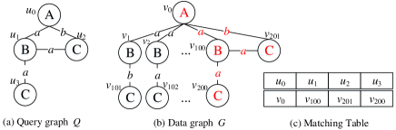
Figure 1: An example of Query Graph and Data Graph

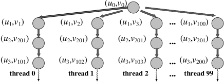
Figure 2: An example of searching tree of $Q$ in $G$

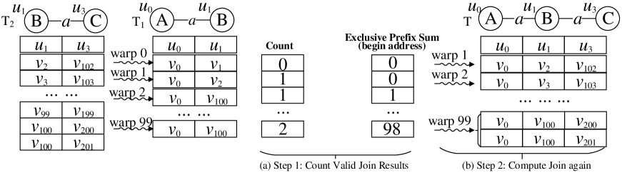
Figure 3: An example of “two-step output scheme”

To the best of our knowledge, two state-of-the-art GPU-based subgraph isomorphism algorithms exist in the literature: GpSM [15] and GunrockSM [16]. In order to avoid the bottlenecks of backtracking [17], they both adopt the breadth-first exploration strategy. They perform edge-oriented computation, where they collect candidates for each edge of $Q$ and join them to find all matches. The edge-based join strategy suffers from high volume of work when implemented on GPU. A key issue is how to write join results to GPU memory in a massively parallel manner. GpSM and GunrockSM employ the “two-step output scheme” [18], as illustrated in Example 1.

Example 1.

Consider $Q$ and $G$ in Figure 1. Tables $T_{1}$ and $T_{2}$ in Figure 3 show the matching edges of $\overline{u_{0}u_{1}}$ and $\overline{u_{1}u_{3}}$, respectively. In order to obtain matches of the subgraph induced by vertices $u_{0}$, $u_{1}$ and $u_{3}$, GpSM performs the edge join $T_{1}\Join T_{2}$. Assume that each processor handles one row in $T_{1}$ for joining. Writing the join results to memory in parallel may lead to a conflict, since different processors may write to the same address.

To avoid this, the naive solution is locking, but that reduces the parallelism. GpSM and GunrockSM use “two-step output scheme” instead. In the first step, each processor joins one row in $T_{1}$ with the entire table $T_{2}$ and counts valid matches (Figure 3(a)). Then, based on the prefix-sum, the output addresses for each processor are calculated. In the second step, each processor performs the same join again and writes the join results to the calculated memory address in parallel (Figure 3(b)).

The two-step output scheme performs the same join twice, doubling the amount of work, and thus suffers performance issues when GPU is short of threads on large graphs. In order to avoid joining twice, we propose a Prealloc-Combine approach, which is based on joining candidate vertices instead of edges. During each iteration, we always join the intermediate results with a candidate vertex set. To write the join results to memory in parallel, we pre-allocate enough memory space for each row of $M$ and perform the vertex join only once. We use vertex rather than edge as the basic join unit, because we cannot estimate memory space for edge join results, which is easy for vertex join. More details are given in Section V.

Vertex join has two important primitive operations: accessing one vertex’s neighbors and set operations. To gain high performance, we propose an efficient data structure (called PCSR, in Section IV) to retrieve a vertex’s neighbors, especially for an edge-labeled graph. Also, adapting to GPU architecture, we design an efficient GPU-based algorithm for set operations.

Putting all these together, we obtain an efficient GPU-friendly subgraph isomorphism solution (called GSI). Our primary contributions are the following:

• We propose an efficient data structure (PCSR) to represent edge-labeled graphs, which helps reduce memory latency.

• Using vertex-oriented join, we propose Prealloc-Combine strategy instead of two-step output scheme, which is significantly more performant.

• Leveraging GPU features, we discuss efficient implementation of set operations, as well as optimizations including load balance and duplicate removal.

• Experiments on both synthetic and real large graph datasets show that GSI outperforms the state-of-the-art approaches (both CPU-based and GPU-based) by several orders of magnitude. Also, GSI has good scalability with graph size scaling to hundreds of millions of edges.

The rest of the paper is organized as follows. Section II gives formal definitions of subgraph isomorphism and background knowledge. In Section III, we introduce the framework of GSI, which consists of filtering phase and joining phase. The optimizations of GSI are discussed in Section VI. Our method can also support other graph pattern semantics, such as homomophism and edge isomorphism; and can process multi-labeled graphs as well. Section VII gives the details of these extensions. Section VIII shows all experiment results and Related works are presented in Section IX. Finally, Section X concludes the paper.

II Preliminaries

TABLE I: Notations

$G,Q$	Data graph and query graph, respectively
$v,u$	Vertex in $G$ and $Q$, respectively
$S(v),S(u)$	Encoding of vertex $v$ or $u$
$N(v),N(u)$	All neighbors of vertex $v$ or $u$
$N(v,l)$	Neighbors of vertex $v$ with edge label $l$
$freq(l)$	Frequency of label $l$ in $G$
$C(u)$	The candidate set of query vertex $u$ in $G$
$M$,$M^{\prime}$	The old and new intermediate result table, each row represents a partial answer, each column correspondings to a query variable
$num(L)$	The number of (valid) elements in $L$
$D=P(G,l)$	Edge label $l$-partitioned subgraph of $G$

In this section, we formally define our problem and review the terminology used throughout this paper. We also introduce GPU background and discuss the challenges for GPU-based subgraph isomorphism computation. Table I lists the frequently-used notations in this paper.

II-A Problem Definition

Definition 1.

(Graph) A graph is denoted as $G=\{V,$ $E,$ $L_{V}$ $L_{E}\}$, where $V$ is a set of vertices; $E\subseteq V\times V$ is a set of undirected edges in $G$; $L_{V}$ and $L_{E}$ are two functions that assign labels for each vertex in $V(G)$ and each edge in $E(G)$, respectively.

Definition 2.

(Graph Isomorphism) Given two graphs $H$ and $G$, $H$ is isomorphic to $G$ if and only if there exists a bijective function $f$ between the vertex sets of $G$ and $H$ (denoted as $f:V(H)\longrightarrow V(G))$, such that

• $\forall u\in V(H),f(u)\in V(G)$ and $L_{V}(u)=L_{V}(f(u))$, where $V(H)$ and $V(G)$ denote all vertices in graphs $H$ and $G$, respectively.

• $\forall\overline{u_{1}u_{2}}\in E(H)$, $\overline{f(u_{1})f(u_{2})}\in E(G)$ and $L_{E}(\overline{f(u_{1})f(u_{2})})$ $=L_{E}(\overline{u_{1}u_{2}})$, where $E(H)$ and $E(G)$ denote all edges in graphs $H$ and $G$, respectively.

• $\forall\overline{u_{1}u_{2}}\in E(G)$, $\overline{f^{-1}(u_{1})f^{-1}(u_{2})}\in E(H)$ and $L_{E}(\overline{f^{-1}(u_{1})f^{-1}(u_{2})})$ $=L_{E}(\overline{u_{1}u_{2}})$

Definition 3.

(Subgraph Isomorphism Search) Given query graph $Q$ and data graph $G$, the subgraph isomorphism search problem is to find all subgraphs $G^{\prime}$ of $G$ such that $G^{\prime}$ is isomorphic to $Q$. $G^{\prime}$ is called a match of $Q$.

This paper proposes an efficient GPU-based solution for subgraph isomorphism search. Without loss of generality, we assume $Q$ is connected and use $v$, $u$, $N(v)$, $N(v,l)$, $num(L)$, and $|A|$ to denote a data vertex, a query vertex, all neighbors of $v$, $\{v^{\prime}|\overline{vv^{\prime}}\in E(G)\wedge L_{E}(\overline{vv^{\prime}})=l\}$, the number of currently valid elements in set $L$, and the size of set $A$, respectively.

II-B GPU Architecture

GPU is a discrete device that contains dozens of streaming multiprocessors (SM) and its own memory hierarchy. Each SM contains hundreds of cores and CUDA (Compute Unified Device Architecture) programming model provides several thread mapping abstractions, i.e., a thread hierarchy.

Thread Hierarchy. Each core is mapped to a thread and a warp contains 32 consecutive threads running in Single Instruction Multiple Data (SIMD) fashion. When a warp executes a branch, it has to wait though only a portion of the threads take a particular branch; this is termed as warp divergence. A block consists of several consecutive warps and each block resides in one SM. Each process launched on GPU (called a kernel function) occupies a unique grid, which includes several equal-sized blocks.

Memory Hierarchy. In Figure 4, global memory is the slowest and largest layer. Each SM owns a private programmable high-speed cache, shared memory, that is accessible by all threads in one block. Although the size of shared memory is quite limited (Taking Titan XP as example, only 48KB per SM), accessing shared memory is nearly as fast as thread-private registers. Access to global memory is done through 128B-size transactions and the latency of each transaction is hundreds of times longer than access to shared memory. If threads in a warp access the global memory in a consecutive and aligned manner, fewer transactions are needed. For example, only 1 transaction is used in coalesced memory access (Figure 5) as opposed to 3 in uncoalesced memory access (Figure 6).

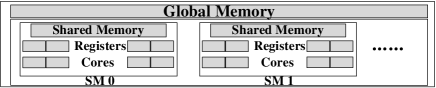
Figure 4: Memory Hierarchy of GPU

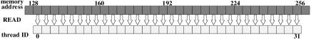
Figure 5: An example of coalesced memory access

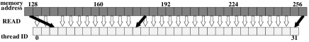
Figure 6: An example of uncoalesced memory access

II-C Challenges of GPU-based Subgraph Isomorphism

Although GPU is massively parallel, a naive use of GPU may yield worse performance than highly-tuned CPU algorithms. There are three challenges in designing GPU algorithms for subgraph isomorphism that we discuss below.

Amount of Work. Let $n$ and $n^{\prime}$ be the number of vertices of $G$ and $Q$, the amount of work is $n^{n^{\prime}}$ in Figure 2. If there are sufficient number of threads, all paths can be fully parallelized. But that is not always possible and too much redundant work will degrade the performance. GpSM’s strategy (filtering candidates and joining them) is better as it prunes invalid matches early. However, Example 1 shows that the two-step output scheme used in GpSM doubles the amount of work in join processing, which is a key issue that must be overcome.

Memory Latency. Large graphs can only be placed in global memory. In subgraph isomorphism, we need to perform $N(v,l)$ extractions many times, and they are totally scattered due to inherent irregularity of graphs [19]. It is hard to coalesce memory access in this case, which aggravates latency.

Load Imbalance. GPU performs best when each processor is assigned the same amount of work. However, neighbor lists vary sharply in size, causing severe imbalance between blocks, warps and threads. Balanced workload is better, because the overall performance is limited by the longest workload.

III Solution Overview

The framework of GSI is given in Figure 7, which consists of filtering and joining phases. Our solution consists of filtering and joining phases. In the filtering phase, a set of candidate vertices in data graph $G$ are collected for each query node $u\in V(Q)$ (denoted as $C(u)$); while, in the joining phase, these candidate sets are joined according to the constraints of subgraph isomorphism (see Definition 3). We discuss how to use GPU to accelerate both phases in the following sections.

Figure 7: Framework of GSI algorithm

III-A Filtering Phase

Generally, a lightweight filtering method with high pruning power is desirable. Since GSI adopts a vertex-oriented strategy, we select candidate vertices $C(u)$ for each query node $u$ in query graph $Q$. More powerful pruning means fewer candidates. Many pruning techniques have been proposed, such as [4]. The basic pruning strategy is based on “neighborhood structure-preservation”: if a vertex $v$ in $G$ can match $u$ in $Q$, the neighborhood structure around $u$ should be preserved in the neighborhood around $v$. In this work, we propose a suitable data structure that fits GPU architecture to implement pruning.

We encode the neighborhood structure around a vertex $v$ in $G$ as a length-$N$ bitvector signature $S(v)$. Generally, it has two parts. The first part is called vertex label encoding that hashes a vertex label into $K$ bits. The second part encodes the adjacent edge labels together with the corresponding neighbor vertex. We divide the $(N-K)$ bits into $\frac{{N-K}}{2}$ groups with 2 bits per group. For each (edge, neighbor) pair $(e,v^{\prime})$ of a vertex $v$, we combine $L_{e}$ and $L_{v^{\prime}}$ (i.e., the labels of edge $e$ and $v^{\prime}$) into a key and hash it to some group. Each group has three states: “00”– no pair is hashed to this group; “01”–only a single pair is hashed to this group; and “11”–more than one pair is hashed to this group. Figure 8(a) illustrates vertex signature $S(v_{0})$ of $G$ in Figure 1. We offline compute all vertex signatures in $G$ and record them in a signature table (see Figure 8(b)). We have the same encoding strategy for each vertex $u$ in $Q$. It is easy to prove that if $S(v)\&S(u)\neq S(u)$, $v$ is definitely not a candidate for $u$ (“&” means “bitwise AND operation”).

Given a query graph $Q$, we compute online vertex signatures for $Q$. For each query vertex $u$, we have to check all vertex signatures in the table (such as Figure 8(b)) to fix candidates. We can perform the filtering in a massively parallel fashion. Furthermore, the natural load balance of accessing fixed-length signatures is suitable for GPU. To further improve the performance, we organize the vertex signature table in column-first instead of row-first. Recall that all threads in a warp read the first element of different signatures in the table, the row-first layout leads to gaps between memory accesses (see Figure 8(c)), i.e., these memory accesses cannot be coalesced. Instead, the column-first layout provides opportunities to coalesce memory accesses (see Figure 8(d)).

Figure 8: Encoding table of data vertices

Figure 9: Vertex-oriented Join Strategy

III-B Joining Phase

The outcome of filtering are candidate sets for all query vertices. In Figure 1, candidate sets are $C(u_{0})=\{v_{0}\}$, $C(u_{1})=\{v_{1},v_{2},...,v_{100}\}$, and $C(u_{2})=C(u_{3})=\{v_{101},v_{102},...,v_{201}\}$. Figure 9 demonstrates our vertex-oriented join strategy. Assume that we have matches of edge $\overline{u_{0}u_{1}}$ in table $M$ and candidate vertices $C(u_{2})$. In $Q$, $u_{2}$ is linked to $u_{0}$ and $u_{1}$ according to the edge labels $b$ and $a$, respectively. Thus, for each record $(v_{i},v_{j})$ in $M$, we read $N(v_{i},b)$ and $N(v_{j},a)$ and do the set operation $N(v_{i},b)\cap N(v_{j},a)\cap C(u_{2})\setminus\{v_{i},v_{j}\}$, where $N(v_{i},b)$ and $N(v_{j},a)$ denote neighbors of $v_{i}$ with edge label $b$ and $v_{j}$ with edge label $a$, respectively. If the result is not empty, new partial answers can be generated, as shown in Figure 9.

Notice that there are two primitive operations: accessing one vertex’s neighbors based on the edge label (i.e., $N(v,l)$ extraction) and set operations. We first present a novel data structure for graph storage on GPU (Section IV). Then, the parallel join algorithm (including the implementation of set operations) is detailed in Section V.

IV Data Structure of Graph: PCSR

Compressed Sparse Row (CSR) [20] is widely used in existing algorithms (e.g., GunrockSM and GpSM) on sparse matrices or graphs, and it allows locating one vertex’s neighbors in $O(1)$ time. Figure 10 shows an example: the 3-layer CSR structure of $G$ in Figure 1. The first layer is “row offset” array, recording the address of each vertex’s neighbors. The second layer is “column index” array, which stores all neighbor sets consecutively. The corresponding weight/label of each edge is stored in “edge value” array. If no edge weight/label exists, we can remove “edge value” array and yield 2-layer CSR structure. To extract $N(v,l)$ in CSR, all neighbors of $v$ must be accessed and checked whether or not corresponding edge label is $l$. Obviously, the memory access latency is very high and it suffers from severe thread underutilization because threads extracting wrong labels are inactive thus wasted. We carefully design a GPU-friendly CSR variant to support accessing $N(v,l)$ efficiently. The complexity of $N(v,l)$ extraction consists of locating and enumerating. In our structures, $N(v,l)$ is stored consecutively, i.e., the complexity of enumerating is the same: $O(|N(v,l)|)$. Thus, we use the time complexity of locating $N(v,l)$ as metric.

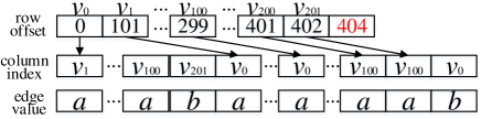
Figure 10: Traditional CSR structure

To speed up memory access, we divide $G$ into different edge label-partitioned graphs (for each edge label $l$, the edge $l$-partitioned $P(G,l)$ is the subgraph $G^{\prime}$ (of $G$) induced by all edges with label $l$). These partitioned graphs are stored independently and edge labels are removed after partitioning. The straightforward way is to store each one using traditional CSR. However, it cannot work well, since vertex IDs in a partitioned graph are not consecutive. For example, the edge partitioned graph $P(G,b)$ only has two edges and four vertices ($v_{0}$,$v_{1}$,$v_{101}$,$v_{201}$). The non-consecutive vertex IDs disable accessing the corresponding vertex in the row offest in $O(1)$ time (by vertex ID). There are two simple solutions:

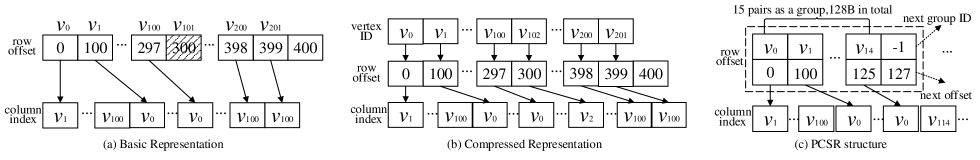
Figure 11: Three Representations of edge $a$-partitioned graph

(1) Basic Representation. The entire vertex set $V(G)$ is maintained in the row offset for each edge partitioned graph CSR, regardless of whether or not a vertex $v$ is in the partitioned graph (see Figure 11(a)). Clearly, this approach can locate a vertex’s neighbors in $O(1)$ time using the vertex ID directly, but it has high space cost: $O(|E(G)|+|L_{E(G)}|\times|V(G)|)$, where $|L_{E(G)}|$ is the number of distinct edge labels. In complex graphs such as DBpedia, there are tens of thousands of different edge labels and this solution is not scalable.

(2) Compressed Representation. A layer called “vertex ID” is added, and binary search is performed over this layer to find corresponding offset (see Figure 11(b)). Obviously, the overall space cost is lowered, which can be formulated as $O(|E(G)|)$. However, this leads to more memory latency. Theoretically, we require $\lceil\log{(|V(G,l)|+1)}\rceil+2$ memory transactions to locate $N(v,l)$, where $|V(G,l)|$ denotes the number of vertices in the edge $l$-partitioned graph $P(G,l)$.

Therefore, neither of the above methods work for a large data graph $G$. In the following we propose a new GPU-friendly data structure to access $N(v,l)$ efficiently, called PCSR (Definition 4). We reorganize the row offset layer using hashing. The row offset layer is an array of hash buckets, called group. Each item hashed to the group is a pair $(v,o_{v})$, where $v$ is a vertex ID and $o_{v}$ is the offset of $v$’s neighbors in column index $ci$. Let $GPN$ be a constant to denote the maximum number of pairs in each group. The last pair is an end flag to deal with the overflow. We require that $2\leq GPN\leq 16$, then one group can be read concurrently by a single memory transaction using one warp.

Definition 4.

PCSR structure. Given an edge $l$-partitioned graph $P(G,l)$, the Partitioned Compressed Sparse Row (PCSR for short) $PCSR(G,l)=\{gl,ci\}$ is defined as follows:

• $ci$ is the column index layer that holds the neighbors.

• $gl=\{g_{i}\}$ is an array of groups and each group is a collection of pairs (no more than $GPN$ pairs).

• Each pair in $g_{i}$ is denoted as $(v,o_{v})$ except for the last pair, where $v$ is a vertex ID and $o_{v}$ is the offset of $v$’s neighbors in $ci$, i.e., a prefix sum of the number of neighbors for vertices. Let $n_{v}$ be the offset of next pair. $v$’s neighbors start at $ci[o_{v}]$ and end before $ci[n_{v}]$. All vertices in one group have the same hash value.

• The last pair $(GID,END)$ is the overflow flag. If $GID$ is -1, it means no overflow; otherwise, overflowed vertices are stored in the $GID$-th group. Note that $g_{i}.END$ is the end position of previous vertex’s neighbors in $ci$, i.e., the first $o_{v}$ in group $g_{i+1}$.

Figure 11(c) is an example of PCSR corresponding to edge $a$-partitioned graph. Let $D$ denote $P(G,l)$, the edge label $l$-partitioned graph. Algorithm 1 builds PCSR for $D$. We allocate $|V(D)|$ groups (i.e. hash buckets) for $gl$ and $|E(D)|$ elements for $ci$ (Line 1). For each node $v$, we hash $v$ to one group using a hash function $f$ (Lines 1-1). If some group $g_{i}$ overflows (i.e., more than $GPN-1$ vertices are hashed to this group), we find another empty group $g_{j}$ and record group ID of $g_{j}$ in the last pair in $g_{i}$ to form a linked list (Lines 1-1). Claim 1 confirms that we can always find empty groups to store these overflowed vertices. Finally, we put neighbors of each vertex in $ci$ consecutively and record their offsets in $gl$ (Lines 1-1).

Claim 1.

When the overflow happens in Line 1 of Algorithm 1, we can always find enough empty groups to store all overflowed vertices.

Proof:

Firstly, once there is a hash conflict of keys, one more empty group arises. Otherwise, let $x$ be the total number of conflicts and $y$ be the number of empty groups, we have $x\neq y$. But it causes a paradox: $|V|-y$ is the number of non-empty groups and the number of all nodes should be equal to $|V|-y+x$, which means $y=x$. Secondly, $\forall g_{i}$, if group $g_{i}$ overflows, it needs to find $\lceil\frac{z}{GPN-1}\rceil-1$ empty groups where $z$ is the number of keys mapped to $g_{i}$. The number of conflicts within group $g_{i}$ is $z-1$ and $g_{i}$ produces $z-1$ empty groups. Obviously, $z-1\geq\lceil\frac{z}{GPN-1}\rceil-1$, so there are enough empty groups for each group’s overflow. These groups do not influence each other, thus the overall empty groups are enough.

Based on PCSR, we compute one vertex’s neighbors according to edge label. An example of computing $N(v_{0},a)$ in Figure 11(c) is given as follows.

1. use the same hash function $f$ to compute the group ID $idx$ that $v_{0}$ maps to, here $idx=0$;

2. read the entire $0$-th group (i.e., $g_{0}$) to shared memory concurrently using one warp in one memory transaction;

3. probe all pairs $(v^{\prime},o_{v^{\prime}})$ in this group ($g_{0}$) concurrently using one warp;

4. we find the first pair (in group $g_{0}$) that contains $v_{0}$. The corresponding offset is 0 and the next offset 100. It means that $ci[0,...,99]$ in the column index layer are $v_{0}$’s neighbors.

Assume that vertex $v$ is hashed to the $i$-th group $g_{i}$. Due to the hash conflict, $v$ may not be in group $g_{i}$. In this case, according to the last pair, we can read another group whose ID is $g_{i}.GID$ and then try to find $v$ in that group. We iterate the above steps until $v$ is found in some group or a group is found whose $g_{i}.GID$ is “-1” (i.e., $v$ does not exist in $D$).

Parameter Setting. The choice of $GPN$ is critical to the performance of PCSR, affecting both time and space. With smaller $GPN$, the space complexity is lower while the probability of group overflow is higher. Once a group overflows, we may need to read more than one group when locating $N(v,l)$, which is more time consuming. With larger $GPN$, the probability of group overflows is reduced, though the space cost rises. Recall that the width of global memory transaction is exactly 128B, so in GSI we set $GPN=16$ to fully utilize transactions. Under this setting, there can be at most 15 keys within a group. The space complexity is a bit high, which can be quantified as $32\times|V(D)|+|E(D)|$. However, it is worthwhile and affordable because at any moment at most one partition is placed on GPU. In addition, under this setting no group overflow occurs in any experiment of Section VIII.

Analysis. Within PCSR, $|V(D)|$ keys are hashed into $|V(D)|$ groups, which is called one-to-one hash [22]. Under this condition, the time complexity of locating $N(v,l)$ can be analyzed by counting memory transactions. It is easy to conclude that the number of memory transactions is decided by the longest conflict list of one-to-one hash function. According to [22], the expectation of longest conflict list’s length is upper bounded by $1+\frac{5\log{|V(D)|}}{\log{\log{|V(D)|}}}$. If $|V(D)|<2^{32}$, the expectation of the maximum length of conflict list is smaller than 45. It means that at most $\left\lceil{\frac{{45}}{{GPN-1}}}\right\rceil=\left\lceil{\frac{{45}}{{15}}}\right\rceil=3$ memory transactions are needed, since one transaction accesses one group and each group contain $GPN$ (=16) valid vertices. This is quite a large data graph. In our experiments, even for graphs with tens of millions of nodes, the longest conflict list’s length is no larger than 13, which means that only one memory transaction is needed to locate $N(v,l)$. In other words, locating $N(v,l)$ is $O(1)$. Furthermore, for each edge label $l$, the space cost of the corresponding PCSR is linear to $P(G,l)$. Thus, we can conclude that the total space of all PCSRs for $G$ is $O(|E(G)|)$. Table II summarizes the comparison, where the time complexity counts both locating and enumerating $N(v,l)$ together.

TABLE II: Efficiency of different data structures

Structure	Time Complexity	Space Complexity
CSR	$O(|N(v)|)$	$O(|E|)$
BR	$O(|N(v,l)|)$	$O(|E|+|L_{E}|\times|V|)$
CR	$O(\log{|V(G,l)|+|N(v,l)|})$	$O(|E|)$
PCSR	$O(|N(v,l)|)$	$O(|E|)$

• BR and CR denote “Basic Representation” and “Compressed Representation”, respectively.

Input: partitioned graph $D=P(G,l)$

Output: PCSR structure of $D$

1 allocate $gl$ array (containing $|V(D)$ groups) and $ci$ array (containing $|E(D)|$ elements);

2 select a hash function $f$, set $pos=0$;

3 foreach node $v$ in $D$ do

4       use $f$ to map $v$ to a group ID $i$;

5      

6foreach group $g_{i}$ in $gl$ do

7       if $g_{i}$ overflows then

8             find enough empty groups $g_{j}$ to store keys of $g_{i}$;

9             set their $GID$s to form a linked list;

10            

11foreach group $g_{i}$ in $gl$ do

12       foreach pair $T_{j}=\{v,o_{v}\}$ in $g_{i}$ do

13             set $o_{v}=pos$ in $T_{j}$;

14             add $N(v)$ to $ci$ from $pos$ on and set $pos=pos+num(N(v))$;

15            

16      set $END=pos$ in $g_{i}$;

17      

18let $gl=\{g_{i}\}$ and return $\{gl,ci\}$ as data structure;

Algorithm 1 Build PCSR structure

V Parallel Join Algorithm

Algorithm 2 outlines the whole join algorithm, where the intermediate table $M$ stores all matches of partial query graph $Q^{\prime}$. In each iteration, we consider one query vertex $u$ and join intermediate table $M$ with candidate set $C(u)$ (Lines 9-11). Heuristically, the first selected vertex has the minimum score $score(u^{\prime})=\frac{C(u^{\prime})}{deg(u^{\prime})}$ (Lines 5-7). In later iterations, we consider the adjacent edge label frequency ($freq(l)$) when selecting the next query vertex to be joined (Lines 12-13).

Input: query graph $Q$, data graph $G$

Output: the final matches of $Q$ in $G$

1 Let $Q^{\prime}$ be the partial query graph, set $Q^{\prime}=\phi$;

2 foreach node $u^{\prime}$ in $Q$ do

3       $score(u^{\prime})=\frac{C(u^{\prime})}{deg(u^{\prime})}$;

4      

5for $i=1$ to $|V(Q)|$ do

6       if $i==1$ then

7             $u_{c}=argmin_{u^{\prime}}{score(u^{\prime})}$;

8             set intermediate table $M=C(u_{c})$ and add $u_{c}$ to $Q^{\prime}$;

9            

10      else

11             $u=argmin_{u^{\prime}\notin Q^{\prime}}\{score(u^{\prime})|u^{\prime}$ is connected to $Q^{\prime}\}$;

12             Call Algorithm 3 to join $M$ with $C(u)$ (generating new intermediate table $M^{\prime}$);

13             set $M=M^{\prime}$, $u_{c}=u$ and add $u$ to $Q^{\prime}$;

14            

15      foreach edge $\overline{u_{c}u^{\prime}}$ in $Q$ do

16             $score(u^{\prime})=score(u^{\prime})\times freq(L_{E}(\overline{u_{c}u^{\prime}}))$;

17            

18return $M$ as final result;

Algorithm 2 The whole join process

Algorithm 3 lists how to process each join iteration (i.e., Line 2 in Algorithm 2). Before discussing the algorithm, we first study some of its key components. Each warp in GPU joins one row of $M$ with candidate set $C(u)$: acquires neighbors of vertices in this row leveraging restrictions on edge labels, and intersects them with $C(u)$ (set intersection). The result of the intersection should remove the vertices in this row (set subtraction), to satisfy the definition of isomorphism.

Let $Q^{\prime}$ be the partial query graph induced by query vertices $u_{0}$ and $u_{1}$. Figure 9 shows the intermediate table $M$, in which each row $m_{i}$ represents a partial match of $Q^{\prime}$. Let $L_{i}^{a}$ and $L_{i}^{b}$ be the neighbor lists of $m_{i}$, e.g., $L_{99}^{a}$ and $L_{99}^{b}$ represents $N(v_{0},a)$ and $N(v_{100},b)$ respectively. For each row $m_{i}$, we assign a buffer ($buf_{i}$) to store temporary results. Assuming that the next query vertex to be joined is $u_{2}$, let us consider the last warp $w_{99}$ that deals with the last row $m_{99}=\{v_{0},v_{100}\}$. There are two linking edges $\overline{u_{0}u_{2}}$ and $\overline{u_{1}u_{2}}$ with edge labels $a$ and $b$, respectively. Warp $w_{99}$ works as follows:

1. Read $v_{0}$’s neighbors with edge label $a$, i.e., $N(v_{0},a)$;

2. Write $buf_{99}=(N(v_{0},a)\setminus\{v_{0},v_{100}\})\wedge C(u_{2})$;

3. Read $v_{100}$’s neighbors with edge label $b$, i.e., $N(v_{100},b)$;

4. Update $buf_{99}=buf_{99}\wedge N(v_{100},b)$.

5. If $buf_{99}\neq\phi$, each item in $buf_{99}$ can be linked to the partial match $m_{99}$ to form a new match of $Q^{\prime}\cup u_{2}$. We write these matches to a new intermediate table $M^{\prime}$.

All warps execute the exact same steps as above in a massively parallel fashion on GPU, which will lead to some conflicts when accessing memory.

Problem of Parallelism. When all warps write their corresponding results to global memory concurrently, conflicts may occur. To enable concurrently outputting results, existing solutions use two-step output scheme, which means the join is done twice. In the first round, the valid join results for each warp are counted. Based on prefix-sum of these counts, each warp is assigned an offset. In the second round, the join process is repeated and join results are written to the corresponding addresses based on the allocated offsets. An example has been discussed in Example 1. Obviously, this approach doubles the amount of work.

Prealloc-Combine. Our solution (Algorithm 3) performs the join only once, which is called “Prealloc-Combine”. Each warp $w_{i}$ joins one row ($m_{i}$) in $M$ with candidate set $C(u)$. Different from existing solutions, we propose “Prealloc-Combine” strategy. Before join processing, for each warp $w_{i}$, we allocate memory for $buf_{i}$ to store all valid vertices that can be joined with row $m_{i}$ (Line 3 in Algorithm 3). A question is how large this allocation should be. Let $Q^{\prime}$ be the partial query graph that has been matched. We select one linking edge $e_{0}=\overline{u_{0}^{\prime}u}$ in query graph $Q$ ($u_{0}^{\prime}\in V(Q^{\prime})$), and $u$ ($\notin V(Q^{\prime})$) is the query vertex to be joined. Assume that the edge label is “$l_{0}$”. As noted above, $m_{i}$ denotes one partial match of query graph $Q^{\prime}$. Assume that vertex $v^{\prime}_{i}$ matches $u_{0}^{\prime}$ in $m_{i}$. It is easy to prove that the capacity of $buf_{i}$ is upper bounded by the size of $N(v^{\prime}_{i},l_{0})$. Based on this observation, we can pre-allocate memory of size $|N(v^{\prime}_{i},l_{0})|$ for each row. Note that this pre-allocation strategy can only work for “vertex-oriented” join, since we cannot estimate the join result size for each row in the “edge-oriented” strategy. During each iteration, the selected edge $e_{0}$ is called the first edge and it should be considered first in Line 3 of Algorithm 3. For example, in Figure 9, $\overline{u_{1}u_{2}}$ is selected as $e_{0}$, thus the allocated size of $buf_{99}$ should be $|N(v_{100},a)|=3$.

Though buffers can be pre-allocated separately for each row (i.e., each row issues a new memory allocation request), it is better to combine all buffers into a big array and assign consecutive memory space (denoted as $GBA$) for them (only one memory allocation request needed). Each warp only needs to record the offset within $GBA$, rather than the pointer to $buf_{i}$. The benefits are two-fold:

(1) Space Cost. Memory is organized as pages and some pages may contain a small amount of data. In addition, pointers to $buf_{i}$ need an array for storage (each pointer needs 8B). Combining buffers together helps reduce the space cost because it does not waste pages and only needs to record one pointer (8B) and an offset array (each offset only needs 4B).

(2) Time Cost. Combined preallocation has lower time overhead due to the reduction in the number of memory allocation requests. Furthermore, the single pointer of $GBA$ can be well cached by GPU and the number of global memory load transactions decreases thanks to the reduction in the space cost of pointer array.

Input: query graph $Q$, current intermediate table $M$ corresponding to the partial matched query $Q^{\prime}$, candidate set $C(u)$ ($u$ is the vertex to be joined), and linking edges $ES$ between $Q^{\prime}$ and $u$.

Output: updated intermediate table $M^{\prime}$

1 Call Algorithm 4 to select the first edge $e_{0}$, and pre-allocate memory $GBA$ and offset array $F$.

2 foreach linking edge $e=\overline{u^{\prime}u}$ in $ES$ do

3       let $l$ be the label of edge $e$ in $Q$;

4       launch a GPU kernel function to join $M$ with $C(u)$ ;

5       forall each row $m_{i}$ (partial match) in $M$ do

6             let $buf_{i}$ be the segment $F_{i}$~$F_{i+1}$ in $GBA$;

7             assign a unique warp $w_{i}$ to deal with $m_{i}$;

8             assume that $v_{i}^{\prime}$ match $u^{\prime}$ in $m_{i}$;

9             if $e$ is the first edge $e_{0}$ then

10                   do set subtraction $buf_{i}=N(v_{i}^{\prime},l)\setminus m_{i}$ ;

11                   do set intersection $buf_{i}=buf_{i}\cap C(u)$ ;

12                  

13            else

14                   do set intersection $buf_{i}=buf_{i}\cap N(v_{i}^{\prime},l)$ ;

15                  

16do prefix-sum scan on $\{num(buf_{i})\}$;

17 allocate memory for new intermediate table $M^{\prime}$;

18 launch a GPU kernel function to link $M$ and $buf_{0,...|M|-1}$ to generate $M^{\prime}$ ;

19 forall partial answer $m_{i}$ in $M$ do

20       read $m_{i}$ into shared memory;

21       assign a unique warp $w_{i}$ to deal with $m_{i}$;

22       forall $z$ in $buf_{i}$ do

23             copy $m_{i}$ and $z$ to the corresponding address of $M^{\prime}$ as a new row;

24            

25return $M^{\prime}$ as the result;

Algorithm 3 Join a new candidate set

Algorithm 4 shows how to allocate buffers $buf_{i}$ for each row $m_{i}$. Assume that there exist multiple linking edges between $Q^{\prime}$ (the matched partial query graph) and vertex $u$ (to be joined). To reduce the size of $|GBA|$, among all linking edges, we select the linking edge $\overline{u_{0}^{\prime}u}$ whose edge label $l_{0}$ has the minimum frequency in $G$ (Line 4). We perform a parallel exclusive prefix-sum scan on each row’s upper bound $|N(v_{i}^{\prime},l_{0})|$ (Lines 4-4), later the offsets ($F[i]$, $\forall 0\leq i<|M|$) and capacity of $GBA$ ($F[|M|]$) are acquired immediately. With the computed capacity, we pre-allocate the $GBA$ and offset array $F[0,...,|M|-1]$ (Line 4). Each buffer $buf_{i}$ begins with the offset $F[i]$.

Let us recall Figure 9, where Figure 9(a) is the process of $GBA$ allocation. First, a parallel exclusive prefix sum is done on $num(L_{i}^{a})$ and the size of $GBA$ is computed (200). Then $GBA$ is allocated in global memory and the address of $buf_{i}$ is acquired. For example, the final row $m_{99}$ has three edges labeled by $a$, thus $num(L_{99}^{a})$ is 3 and the beginning address of $buf_{99}$ in $GBA$ is 197. However, if $\overline{u_{0}u_{2}}$ is selected as the first edge $e_{0}$, we can yield smaller $|GBA|$ (100). The label $b$ of $\overline{u_{0}u_{2}}$ is more infrequent than $a$, thus heuristically it is superior, as illustrated in Algorithm 4. For ease of presentation, we still assume that $\overline{u_{1}u_{2}}$ is selected as $e_{0}$ in Figure 9.

In each join iteration, Algorithm 3 handles all linking edges between $Q^{\prime}$ and $u$. It allocates $GBA$ (Line 3), processes linking edges one by one (Lines 3-3), and finally generates a new intermediate table $M^{\prime}$(Lines 3-3). Obviously, $GBA$ is allocated only once in Algorithm 3 and no new temporary buffer is needed. Figure 9(a) performs the $GBA$ allocation by edge $\overline{u_{1}u_{2}}$ and Figure 9(b) finishes set operations. Correspondingly, edge $\overline{u_{1}u_{2}}$ is joined first. For example, $L_{99}^{a}$ subtracts $m_{99}$ and the result is $\{v_{200},v_{201}\}$, which are stored in $buf_{99}$ (Line 3). Next, for each valid element $x$ in $buf_{99}$, we check its existence in candidate set of $u_{2}$ (Line 3). The second edge is $\overline{u_{0}u_{2}}$ and it is processed by Line 3, where $buf_{99}$ is further intersected with $L_{99}^{b}$ and the result is $\{v_{201}\}$, i.e., $num(buf_{99})=1$. We acquire the matching vertices of each row $m_{i}$ in $buf_{i}$, then a new prefix sum is performed to obtain size and offsets of $M^{\prime}$ (Line 3). After $M^{\prime}$ is allocated, $w_{i}$ copies extensions of $m_{i}$ to $M^{\prime}$ (Lines 3-3).

Input: query graph $Q$, current intermediate table $M$ corresponding to the partial matched query $Q^{\prime}$, candidate set $C(u)$ ($u$ is the query vertex to be joined), and linking edges $ES$ between $Q^{\prime}$ and $u$.

Output: Allocated memory $GBA$ and Offset arrary $F$.

1 Among all edges in $ES$, select edge $e_{0}=\overline{u_{0}^{\prime}u}$, whose edge label $l_{0}$ has the minimum frequency in $G$.

2 Set offset $F[0]$=0;

3 foreach row $m_{i}$ in $M$, $i=0,...,|M|-1$ do

4       Assume vertex $v_{i}^{\prime}$ matches query vertex $u_{0}^{\prime}$ in row $m_{i}$.

5       $F[i+1]$=$F(i)$+$|N(v_{i}^{\prime},l_{0})|$. // Do exclusive prefix-sum scan.

6      

7Let $|GBA|=F[|M|]$;

8 Allocate consecutive memory with size $|GBA|$ and let $GBA$ record the beginning address.

Return $GBA$ and offset array $F[0,...,|M|-1]$.

Algorithm 4 Function: Pre-allocate Memory

GPU-friendly Set Operation. In Algorithm 3, set operations (Lines 3,3,3) are in the innermost loop, thus frequently performed. Traditional methods (e.g., [23]) all target the intersection of two lists. However, in our case there are many lists of different granularity for set operations. A naive implementation launches a new kernel function for each set operation and uses traditional methods to solve it. This method performs bad, so we propose a new GPU-friendly solution.

There are three granularities: small (partial match $M_{i}$), medium (neighbor list $N(v,l)$) and large (candidate set $C(u)$). We use one warp for each row and design different strategies for these lists:

• For small list $M_{i}$, we cache it on shared memory until the subtraction finishes.

• For medium list $N(v,l)$, we read it batch-by-batch (each batch is 128B) and cache it in shared memory, to minimize memory transactions.

• For large list $C(u)$, we first transform it into a bitset, then use exactly one memory transaction to check if vertex $v$ belongs to $C(u)$.

Lines 3 and 3 can be combined together. After subtraction, the check in Line 3 is performed on the fly.

We also add a write cache to save write transactions, as there are enormous invalid intermediate results which do not need to be written back to $buf_{i}$. It is exactly 128B for each warp and implemented by shared memory. Valid elements are added to cache first instead of written to global memory directly. Only when it is full, the warp flushes its cached content to global memory using exactly one memory transaction.

VI Optimizations

There are two more optimizations in Algorithm 3: improving workload balance and elimination of duplicate vertices. We discuss these below.

VI-A Load Balance

In Algorithm 3, load imbalance mainly occurs in Lines 3 and 3, where neighbor set sizes of all rows are distributed without attention to balance. We propose to balance the workload using the following method (4-layer balance scheme): (1) Extract workloads that exceed $W_{1}$, and dynamically launch a new kernel function to handle each one; (2) Control the entire block to deal with all workloads larger than $W_{2}$; (3) In each block, all warps add their tasks exceeding $W_{3}$ to shared memory and then divide them equally; and (4) Each warp finishes remaining tasks of the corresponding row.

The first strategy limits inter-block imbalance; the next two limit imbalance between warps. $W_{2}$ should be set as the block size of CUDA, while $W_{1}$ and $W_{3}$ are parameters that should be tuned ($W_{1}>W_{2}>W_{3}>32$). This method is superior to merging all tasks and dividing them equally [24], because it avoids the overhead of merging tasks into work pool.

VI-B Duplicate Removal

In Figure 9, the first elements of all rows are all $v_{0}$ and each row does the same operation: extracting $N(v_{0},a)$. To reduce redundant memory access, we propose a heuristic method to remove duplicates within a block. If rows $x$ and $y$ have a common vertex $v$ in the same column, we let the two warps of $x$ and $y$ ($wx$ and $wy$) share the input buffer (placed in shared memory) of $N(v,l)$. For the shared input buffer, only a single warp (e.g., warp $wx$) reads neighbors into buffer. Other warps wait for the input operation to finish and then all warps perform their own operations. Algorithm 5 gives implementation details.

Input: vertex $v_{i}$ and input buffer $buf_{i}$ for each warp $w_{i}$

1 foreach warp $w_{i}$ in the block do

2       $id[i]$ = $v_{i}$;

3       synchronize all warps within the block;

4       use $w_{i}$ to find the first occurrence $j$ of $v_{i}$ in $id[]$;

5       $addr[i]=j$;

6      

7foreach batch $b_{i}$ of $buf_{i}$ do

8       if $addr[i]==i$ then

9             use $w_{i}$ to read batch $b_{i}$ into buffer $buf_{i}$;

10            

11      synchronize all warps within the block;

12       each warp $w_{i}$ processes the batch located in $buf_{addr[i]}$;

13      

Algorithm 5 Duplicate removal within each block

VII Extensions

VII-A Homomorphism and edge isomorphism

Our method can be generalized to support homomorphism and edge isomorphism subgraph query semantics. Both of these semantics are equally important as vertex isomorphism and to all foresight will be supported by upcoming query languages standards. We briefly discuss them below.

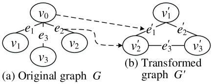
Figure 12: Example of edge isomorphism

According to [6], homomorphism semantics drops the constraint in subgraph isomorphism that two different query vertices in $Q$ should be matched to two distinct vertices in the data graph $G$. Therefore, to support homomorphism, we only need to eliminate the set subtraction operation (Line 10 in Algorithm 3) in our joining phase.

According to [25], the semantics of edge isomorphism requires that two edges (in $Q$) share a common vertex of $Q$ if and only if the mapping edges (in $G$) share a common vertex of $G$. To support it, we can transform the original graph $G$ into a new graph $G^{\prime}$. Each edge $e$ of $G$ is transformed into a vertex $v^{\prime}$ of $G^{\prime}$, and each vertex $v$ is transformed into several edges of $G^{\prime}$. Figure 12 shows an example. Let $e_{1}=\overline{v_{0}v_{1}}$, $e_{2}=\overline{v_{0}v_{2}}$ and $e_{3}=\overline{v_{0}v_{3}}$ be three edges in $G$; we transform $e_{1}$, $e_{2}$ and $e_{3}$ into three vertices $v_{1}^{\prime}$, $v_{2}^{\prime}$ and $v_{3}^{\prime}$ of $G^{\prime}$. Since $e_{1}$ and $e_{2}$ share the common vertex $v_{0}$, we transform $v_{0}$ into an edge $e_{1}^{\prime}=\overline{v_{1}^{\prime}v_{2}^{\prime}}$ of $G^{\prime}$. The same thing happens between $e_{1}$ and $e_{3}$, $e_{2}$ and $e_{3}$, which means $v_{0}$ is transformed into $e_{1}^{\prime}$, $e_{2}^{\prime}$ and $e_{3}^{\prime}$. Such transformation is also performed on query graph $Q$ to generate $Q^{\prime}$. Then, we can perform subgraph isomorphism of $Q^{\prime}$ on $G^{\prime}$ to get results $R^{\prime}$. The final results $R$ of searching $Q$ on $G$ can be acquired via reverse transformation of $R^{\prime}$.

VII-B Process vertex/edge multi-labels

In some situations, a vertex (or an edge) may have multiple labels. For vertex/edge multi-labels, we should first change the definition of subgraph isomorphism. A proper change is: For each vertex $u$/edge $\overline{u_{1}u_{2}}$ in query graph $Q$, assume that the matching vertex/edge is denoted as $f(u)$ and $f(\overline{u_{1}u_{2}})$, respectively and we require that $L_{V}(u)\subseteq L_{V}(f(u))$ and $L_{E}(\overline{u_{1}u_{2}})\subseteq L_{E}(\overline{f(u_{1})f(u_{2})})$.

Under the above definition, the data structures and algorithms in both filtering and join phases in GSI should be adjusted as follows.

(1) For vertices with multiple labels, we only need to modify the filtering phase. In the case of single-label vertex $v$, we use a special strategy to process vertex label, which stores the label directly in the beginning of $v$’s signature (see Section VIII-B. However, if $v$ has multiple labels, this special strategy can not be used, i.e., we need to use hash functions for vertex labels. Given a data vertex $v$ (or query vertex $u$), we can hash all labels of $v$ (or $u$) into its signature, then perform the original filtering phase. The main difference is that candidate sets must be refined by verifying the containment of vertex labels, which can be finished quickly on GPU. Given a query vertex $u$ and its candidate set $C(u)$, each thread can examine each candidate $v$ in $C(u)$, checking if the label set of $v$ contains the label set of $u$. After the refinement, the joining phase can work properly because it does not consider vertex labels.

(2) For edges with multiple labels, we work as follows. Given graphs $Q$ and $G$ with multiple edge labels, we transform them as multiple-edge graphs $Q^{\prime}$ and $G^{\prime}$, respectively, where each edge has a single edge label (as shown in the following Figure 13). The whole GSI algorithm does not need be changed to handle the multiple-edge graph, as GSI always processes one edge at a time (Line 3-13 of Algorithm 3).

Figure 13: Example of multi-labeled edge

VIII Experiments

In this section, we evaluate our method (GSI) against state-of-the-art subgraph matching algorithms, such as CPU-based solutions VF3 [10], CFL-Match [8], CBWJ [26], and GPU-based solutions GpSM and GunrockSM. We also include two state-of-the-art GPU-based RDF systems (MAGiQ [27] and Wukong+G [28]) in the experiments. Note that RDF systems are originally designed for SPARQL queries whose semantic is subgraph homomorphism; we extend them to support subgraph isomorphism. All experiments are carried out on a workstation running CentOS 7 and equipped with Intel Xeon E5-2697 2.30GHz CPU and 188G host memory, NVIDIA Titan XP with 30 SMs (each SM has 128 cores and 48KB shared memory) and 12GB global memory.

VIII-A Datasets and Queries

The experiments are conducted on both real and synthetic datasets. The statistics are listed in Table III. Enron email communication network (enron), the Gowalla location-based social network (gowalla), patent citation network (patent) and the road_central USA road network (road) are downloaded from SNAP [29]. Large RDF graphs, such as DBpedia [30] and WatDiv (a synthetic RDF benchmark [31]), are also used.

TABLE III: Statistics of Datasets

Name	$|V|$	$|E|$	$|L_{V}|$	$|L_{E}|$	MD1	Type2
enron	69K	274K	10	100	1.7K	rs
gowalla	196K	1.9M	100	100	29K	rs
patent	6M	16M	453	1K	793	rs
road	14M	16M	1K	1K	8	rm
DBpedia	22M	170M	1K	57K	2.2M	rs
WatDiv	10M	109M	1K	86	671K	s

• $|L_{V}|$ and $|L_{E}|$ denote the number of vertex label and edge label, respectively.

• Maximum degree of the graph.

• Graph type: r:real-world, s:scale-free, and m:mesh-like.

Since most graphs do not contain vertex/edge labels except for edge labels in RDF datasets and vertex labels in patent dataset, we assign labels following the power-low distribution. The default numbers of vertex/edge labels are given in Table III. To generate a query graph, we perform the random walk over the data graph $G$ starting from a randomly selected vertex until $|V(Q)|$ vertices are visited. All visited vertices and edges (including the labels) form a query graph. The same query graph generation approaches are also used in [32, 33].

For each query size $|V(Q)|$, we generate 100 query graphs and report the average query running time. Note that the default query size $|V(Q)|$ is 12 in the following experiments. In Section VIII-F, we also evaluate GSI with respect to the number of vertex/edge labels and query size.

VIII-B Evaluating Filtering Strategy

Let us recall the encoding technique in Section III-A. The neighborhood structure around each vertex $v$ is encoded into a length-$N$ bitvector signature $S(v)$. Furthermore, $K$ of $N$ bits denote vertex $v$’s label and the left bits correspond to $v$’s adjacent edges and neighbors (an example is given in Figure 8(a)). In our experiments, we set $N$=512 and $K$=32. By varying the encoding length, we can balance the filtering time and the pruning power.

To verify the effectiveness of our encoding, we compare it with the pruning techniques (used in GpSM and GunrockSM) that are based on node label and degree. The metrics include time cost and the size of the minimum candidate set, because the joining phase always begins from the minimum candidate set. Experimental results (Table IV) show that our encoding strategy not only obtains much smaller candidate sizes (reduces 10-100 times) than the filtering in existing algorithms but also consumes less pruning time. The superiority of our filtering method is due to the careful design of signature structure on GPU. Natural load balance is achieved, and the column-first layout of vertex signatures also brings performance improvement due to coalesced memory access.

TABLE IV: Performance of different filtering strategies

Dataset	Minimum $|C(u)|$			Time (ms)
	GpSM	GSM1	GSI	GpSM	GSM	GSI
enron	2,246	2,270	111	24	20	9
gowalla	153	1,072	90	31	24	16
patent	2,298	3,401	25	781	569	354
road	8	2,544	7	259	394	187
WatDiv	871	12,145	604	290	252	201
DBpedia	138	11,405	132	410	494	407

• The filtering strategy of GunrockSM.

TABLE V: Performance of techniques in join phase

Dataset

Global Memory Load Transactions

Query Response Time (ms)

GSI-1

+DS2

drop

+PC3

drop

+SO4

drop

GSI-

+DS

speedup

+PC

speedup

+SO

speedup

enron

3M

2.1M

30%

1.6M

25%

656K

59%

573

274

2.1x

176

1.6x

28

6.3x

gowalla

3.2M

2M

38%

1.3M

33%

848K

39%

353

172

2.1x

88

2.0x

69

1.3x

patent

3.5M

2.4M

31%

1.8M

25%

1.6M

11%

3K

1.4K

2.1x

700

2.0x

524

1.3x

road

3.4M

2.2M

35%

1.7M

22%

1.6M

5%

2.4K

675

3.6x

456

1.5x

456

1.0x

WatDiv

40M

30M

25%

21M

28%

13M

39%

43K

31K

1.4x

25K

1.2x

4.4K

5.7x

DBpedia

53M

31M

42%

24M

21%

14M

43%

85K

48K

1.8x

36K

1.3x

6K

6.0x

• Basic GSI implementation with traditional CSR structure, two-step scheme and naive set operation.

• Add techniques to GSI- one by one: PCSR structure, Prealloc-Combine strategy and GPU-friendly set operation.

VIII-C Evaluating Join Phase

We evaluate three techniques of the join phase in GSI: PCSR structure, the Prealloc-Combine strategy and GPU-friendly set operation. Table V shows the result, where GSI- is the basic implementation with traditional CSR structure, two-step output scheme and naive set operation. Two metrics are compared: (1) the number of transactions for reading data from global memory (GLD); (2) the time cost of answering subgraph search query. We add techniques to GSI- one by one, and compare the performance of each technique with previous implementation. For example, in Table V, the column “+SO” is compared with the column “+PC” to compute GLD drop and speedup. After adding these techniques, we denote the implementation as GSI.

TABLE VI: Comparison of CR and PCSR

Dataset	GLD			Time (ms)
	CR	PCSR	drop	CR	PCSR	speedup
enron	2.4M	2.1M	13%	311	274	1.1x
gowalla	2.5M	2M	20%	212	172	1.2x
patent	3.2M	2.4M	25%	1.8K	1.4K	1.3x
road	3.0M	2.2M	27%	873	675	1.3x
WatDiv	46M	30M	35%	42K	31K	1.4x
DBpedia	37M	31M	16%	56K	48K	1.2x

VIII-C1 Performance of PCSR structure

To verify the efficiency of PCSR in Section IV, we compare it with traditional CSR structure. We set the bucket size as 128B and find that the maximum length of conflict list is below 15, even on the largest dataset. Therefore, with PCSR structure, GSI always finds the address of $N(v,l)$ within one memory transaction, which is a big improvement compared to traditional CSR.

Table V shows that PCSR brings an observable drop of GLD (about 30%), and nearly 2.0x speedup. The least improvement is observed on WatDiv due to small $|L_{E}|$, while on other datasets the power of PCSR is tremendous, achieving more than 1.8x speedup. The superiority of PCSR is two-fold: (1) fewer memory transactions are needed, as presented in Table II; and (2) threads are fully utilized while traditional CSR suffers heavily from thread underutilization.

We also compare PCSR with “Compressed Representation” (CR) in Table VI. On all datasets, at least 13% drop of GLD and 1.1x speedup are achieved. WatDiv delivers the best performance, where CR even has higher GLD than traditional CSR. PCSR has no advantage over CR when enumerating $N(v,l)$, and the only difference is locating. WatDiv has the minimum number of edge labels, thus its edge label-partitioned graphs are very large, leading to high cost of locating for CR. The “Basic Representation” (BR) consumes too much memory to run on large graphs with hundreds of edge labels.

TABLE VII: Performance of Write Cache

Dataset	Global Memory Store Transactions			Query Response Time (ms)
	no cache	write cache	drop	no cache	write cache	drop
enron	25,371	23,056	9%	117	28	76%
gowalla	43,304	37,147	14%	78	69	12%
road	70,430	65,500	7%	456	456	0%
WatDiv	110,744	86,934	22%	8,396	4,425	47%
DBpedia	248,670	90,284	64%	12,194	6,148	50%

VIII-C2 Performance of Parallel Join Algorithm

In our vertex-oriented join strategy, there are two main parts: the Prealloc-Combine strategy (PC) and GPU-friendly set operation (SO).

To evaluate Prealloc-Combine strategy, we implement the two-step output scheme [15] as the baseline. Table V shows that on all datasets, PC obtains more than 21% drop of GLD and 1.2x speedup. The gain originates from the elimination of double work during join, which also helps reduce GLD, thus further boosts the performance. It must be pointed out that PC can reduce the amount of work by at most half, thus there is no speedup larger than 2.0x.

To evaluate our GPU-friendly set operation, we compare with naive solution: finish each set operation with a new kernel function. Table V shows that SO reduces GLD by about 40%; consequently, it leads to more than 1.3x speed up. On patent and road, the improvement is not apparent because their neighbor lists are relatively small. SO also eliminates the cost of launching many kernel functions.

SO performs best on enron, WatDiv and DBpedia, showing >5.7x speedup. The reason is that write cache performs best on these graphs, thus saving lots of global memory store transactions (GST). On other graphs, the gain of write cache is small because they have fewer matches, thus perform fewer write operations.

VIII-D Evaluating Optimization Techniques in GSI

We evaluate the two optimization strategies proposed in Section VI and give the result in Table VIII, where column “+DR” is compared with column “+LB”. After adding the two optimizations, we denote the implementation as GSI-opt.

VIII-D1 Performance of Load Balance scheme

The 4-layer balance scheme (LB) in Section VI-A does not save global memory transactions, or the amount of work. However, it improves the performance by assigning workloads to GPU processors in a more balanced way. We verify its efficiency by comparing it with the strategy used in [24]. $W_{2}$ should be equal to the block size of CUDA (1024), and empirically we set $W_{1}=4W_{2}=16W_{3}=4096$.

On the four smaller datasets, LB does not show much advantage because the time cost is already very low (less than 0.6 seconds) and the load imbalance is slight. But on other datasets, LB brings tremendous performance gain, i.e., more than 2.7x speedup. This demonstrates that our strategy is especially useful on large scale-free graphs, due to the existence of severely skewed workloads. Note that though patent is scale-free, its maximum degree is small, which limits the effect of LB.

TABLE VIII: Performance of optimizations

Dataset$\backslash$Time(ms)	GSI	+LB1	speedup	+DR2	speedup
enron	28	28	1.0x	28	1.0x
gowalla	69	69	1.0x	68	1.0x
patent	524	466	1.1x	465	1.0x
road	456	456	1.0x	456	1.0x
WatDiv	4.4K	1.3K	3.4x	1K	1.3x
DBpedia	6K	2.2K	2.7x	2K	1.1x

• Add load balance techniques to GSI.

• Add duplicate removal method to GSI + LB.

VIII-D2 Performance of Duplicate Removal method

Using the duplicate removal method (DR) in Section VI-B, input is shared within a block so the amount of work should be reduced theorectically. Compared with baseline (no duplicate removal), Table VIII shows 1.3x and 1.1x speedup on WatDiv and DBpedia, respectively. Besides, GLD is also lower with DR, but its comparison is omitted here.

This experiment shows that DR really works, though the improvement is small. The bottleneck is the region size that DR works on, i.e., a block. Even with the block size set to maximum (1024), DR can only remove duplicates within 32 rows since we use a warp for each row.

TABLE IX: Performance of Duplicate Removal method

Dataset	Global Memory Load Transactions			Query Response Time(ms)
	with duplicates	duplicate removal	drop	with duplicates	duplicate removal	drop
enron	656K	630K	4%	28	28	0%
gowalla	848K	824K	3%	69	68	1%
road	1.66M	1.61M	3%	456	456	0%
WatDiv	13M	10M	21%	1.3K	1K	17%
DBpedia	14M	10M	23%	2.2K	2K	9%

VIII-E Comparison of GSI with counterparts

Overall Performance. The results are given in Figure 14, where GSI and GSI-opt represent implementations without and with optimizations (in Section VI), respectively. Note that there is no bar if the corresponding time exceeds the threshold of 100 seconds. In all experiments, GPU solutions beat CPU solutions as expected due to the power of massive parallelism.

Considering existing GPU solutions only, there is no clear winner between four counterparts, but they all fail to compete with GSI. GSI runs very fast on the first four datasets, answering queries within one second. On WatDiv and DBpedia, GSI achieves more than 4x speedup over counterparts.

Focusing on our solution, on the first four datasets, GSI-opt is close to GSI; while on the latter two, GSI-opt shows more than 3x speedup. To sum up, our solution outperforms all counterparts on all datasets by several orders of magnitude.

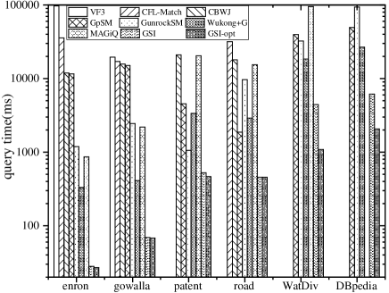
Figure 14: Performance Comparison on all datasets

Scalability. We generate a series of RDF datasets using the WatDiv benchmark. These scale-free graphs are named watdiv10M, watdiv20M,…,watdiv210M, with the number of vertices and edges growing linearly as the number in the name. CPU solutions fail to run even on the smallest watdiv10M dataset, thus, we only compare GPU solutions and draw the curves in Figure 15(a). Note that the curve stops if the memory consumption exceeds GPU capacity or the time exceeds 100s. The curves of four counterparts are above the curves of GSI and GSI-opt. Besides, they rise sharply as the data size grows larger. In contrast, GSI-opt rises much more slowly.

After watdiv210M, all algorithms fail on most queries due to the limitation of GPU memory capacity. The counterparts stop much earlier because they have larger candidate tables and intermediate tables. Due to its efficient filter, GSI occupies less memory, thus scaling to larger graphs. Furthermore, during each join iteration of GSI, only an edge label-partitioned graph is needed on GPU. In summary, GSI not only outperforms others by a significant margin, but also shows good scalability so that graphs with hundreds of millions of edges for subgraph query problem are now tractable.

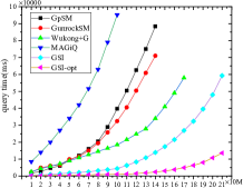
(a) Scalability with the data size

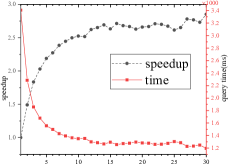
(b) Scalability with the number of SMs

Figure 15: Scalability Test

We also evaluate the scalability of GSI with the number of SMs. In order to control the number of running SMs, we limit the number of blocks launched and withdraw dynamic kernels (see Section VI-A), which may degrade the performance. We choose WatDiv (see Table III) and show the result in Figure 15(b). With the number of SMs increasing from 1 to 30, the response time drops continuously, though with some tiny fluctuations. The time curve drops fast in the beginning, but slows down gradually, corresponding to the sub-linear speedup curve. The maximum speedup is 2.85, and is limited by the irregularity of graphs and GPU memory bandwidth, which cause severe load imbalance and high memory latency.

VIII-F Vary the number of labels and query size

In this section, we explore the influence of number of labels and query size. We use GSI-opt and select gowalla as the benchmark. By default, the number of vertex and edge labels are both 100, and all queries have 12 vertices.

We vary the number of labels and show results in Figure 16(a). As the number of labels increases, run time decreases. The “vertex label num” line shows sharper drop because larger $|L_{V}|$ directly reduces the sizes of candidate sets. However, after $|L_{V}|>100$, the drop quickly slows down to zero as candidate sets are small enough to be fully parallelized. Similarly, larger $|L_{E}|$ also helps reduce $|C(u)|$ due to improved pruning power of labeled edges. In addition, the size of $|N(v,l)|$ is also lowered as $|L_{E}|$ grows. This is the reason that run time keeps dropping, though the speed also changes after $|L_{E}|>100$.

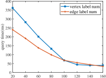
(a) Vary the number of vertex and edge labels

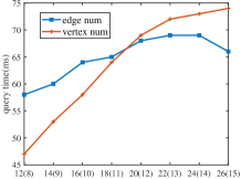
(b) Vary the number of edges and vertices in $Q$

Figure 16: Experiments of label number and query size

As for query size, we first fix $|V(Q)|=12$ and vary the number of edges, then fix $|E(Q)|=2\times|V(Q)|$ and vary the number of vertices. Figure 16(b) shows the result, where unenclosed X-axis numbers denote the number of edges, and the X-axis numbers enclosed in parentheses denote the number of vertices. In the first case, run time rises slowly, because the cost of processing extra edges is marginal. After $|E(Q)|>24$, a small drop occurs as there are enough edges to provide stronger pruning potential. In the second case, an observable increase can be found because in our vertex-oriented join strategy, larger $|V(Q)|$ means more join iterations. However, the rise slows down after $|V(Q)|\geq 13$. Generally, larger query graph results in fewer matches, thus the cost of each join iteration is lower.

VIII-G Distribution of query time and result size

In addition to average time, using GSI-opt, we also show the distribution of query time and result size in Figure 17.

For query time, the relative height of boxes corresponds to the results of average time in Figure 14. Due to the irregularity of graphs, a few outliers exist. On WatDiv and DBpedia, the mean is above the major part (the box area) because the cost of outliers is too high.

For result size, gowalla, patent and road deliver the minimum value, which limits the speedup by write cache. It must be noted that query time is not decided by result size. Besides, the data skew on the latter two graphs are more severe, thus outliers are far above the box.

(a) Box plot of query response time

(b) Box plot of query result size

Figure 17: Distribution of query response time and query result size

VIII-H Additional Experiments

We report the loading time (from host to GPU) of GSI on all datasets: 1ms, 5ms, 106ms, 120ms, 144ms, 178ms. Besides, we record the maximum memory consumption of GPU algorithms in Table X, including host and GPU memories. For CPU algorithms, only host memory consumption is reported in Table XI. Note that “NAN” means an algorithm cannot end in a reasonable time. Besides, CPU solutions all fail on WatDiv and DBpedia. Obviously, backtracking solutions (VF3 and CFL-Match) occupy less memory.

GPU solutions that are based on BFS have larger memory consumption on both host and GPU. Compared to counterparts, GSI consumes more host memory due to the maintainance of signature table and PCSR structures. However, GSI consumes less GPU memory because it has smaller candidate/intermediate tables and in each iteration only an edge label-partitioned graph is needed on GPU.

TABLE X: Memory consumption of GPU algorithms

Dataset	Host Memory					GPU Memory
	GpSM	GunrockSM	Wukong+G	MAGiQ	GSI	GpSM	GunrockSM	Wukong+G	MAGiQ	GSI
enron	154M	181M	174M	284M	160M	1.3G	1.4G	667M	721M	661M
gowalla	592M	712M	599M	367M	466M	2.4G	2.8G	1.8G	725M	685M
patent	1.0G	1.3G	1.3G	1.5G	663M	3.5G	3.7G	2.1G	1.1G	915M
road	1.8G	2.0G	2.1G	2.2G	1.1G	3.6G	3.6G	2.3G	1.3G	1.2G
WatDiv	4.4G	5.7G	4.7G	6.9G	8.5G	7.3G	7.7G	7.5G	5.6G	4.9G
DBpedia	6.9G	8.2G	8G	NAN	14G	9.0G	9.6G	9.6G	NAN	8.1G

TABLE XI: Memory consumption of CPU algorithms

Algorithm$\backslash$Dataset	enron	gowalla	patent	road
VF3	10M	39M	NAN	NAN
CFL-Match	21M	62M	NAN	416M
CBWJ	15M	64M	817M	1.5G

IX Related Work

CPU-based subgraph isomorphism. Ullmann [34] and VF2 [35] are the two early efforts; Ullmann uses depth-first search strategy, while VF2 considers the connectivity as pruning strategy. Most later methods (e.g., [14, 13]) pre-compute some structural indices to reduce the search space and optimize the matching order using various heuristic methods. TurboISO [11] merges similar query nodes and BoostISO [12] extends this idea to data graph. CFL-Match [8] defines a Core-Forest-Leaf decomposition and select the matching order based on minimal growth of intermediate table. VF3 [10] is an improvement of VF2, which leverages more pruning rules (node classification, matching order, etc.) and favors dense queries. EmptyHeaded [36] and CBWJ [26] are based on worst-case optimal join [37]; CBWJ achieves better performance. Unfortunately, these sequential solutions perform terrible on large graphs, due to exponential search space.

GPU-based subgraph isomorphism. The first work is [38], which finds candidates for STwigs [39] first and joins them. However, STwig-based framework may not be suitable for GPU due to large intermediate results. Later, GPUSI [40] transplants TurboISO to GPU. Different candidate regions are searched in parallel, but its performance is limited by depth-first search within each region. All backtracking-based GPU algorithms have problems of warp divergence and uncoalesced memory access, as analyzed in [17].

GpSM [15] and GunrockSM [16] outperform previous works by leveraging breadth-first search, which favors parallelism. Their routines are already introduced in Section I. They both adopt two-step output scheme to write join results, and do not utilize features of GPU architecture. Therefore, they have problems of high volume of work, long latency of memory access and severe workload imbalance. In summary, GpSM and GunrockSM both lack optimizations for challenges presented in Section II-C.

MAGiQ [27] and Wukong+G [28] are two GPU-based RDF systems that supports SPARQL queries. Wukong+G develops efficient swapping mechanism between CPU and GPU, while MAGiQ utilizes existing CUDA libraries of linear algebra for filtering. They have no optimization for table join, which marks them inefficient.

X Conclusions

We introduce an efficient algorithm (GSI), utilizing GPU parallelism for large-scale subgraph isomorphism. GSI is based on filtering-and-joining framework and optimized for the architecture of modern GPUs. Experiments show that GSI outperforms all counterparts by several orders of magnitude. Furthermore, all pattern matching algorithms using $N(v,l)$ extraction can benefit from the PCSR structure. The Prealloc-Combine strategy also sheds new light on join optimization.

References

- [1] X. Yan, P. S. Yu, and J. Han, “Graph indexing: a frequent structure-based approach,” in SIGMOD, 2004.
- [2] J. Pérez, M. Arenas, and C. Gutierrez, “Semantics and complexity of sparql,” ACM Transactions on Database Systems (TODS), 2009.
- [3] O. Lassila, R. R. Swick et al., “Resource description framework (rdf) model and syntax specification,” W3c Recommendation, 1998.
- [4] L. Zeng and L. Zou, “Redesign of the gstore system,” Frontiers Comput. Sci., 2018.
- [5] M. R. Garey and D. S. Johnson, Computers and Intractability: A Guide to the Theory of NP-Completeness. W. H. Freeman, 1979.
- [6] D. Conte, P. Foggia, C. Sansone, and M. Vento, “Thirty years of graph matching in pattern recognition,” IJPRAI, 2004.
- [7] J. Kim, H. Shin, W. Han, S. Hong, and H. Chafi, “Taming Subgraph Isomorphism for RDF Query Processing,” PVLDB, 2015.
- [8] F. Bi, L. Chang, X. Lin, L. Qin, and W. Zhang, “Efficient subgraph matching by postponing cartesian products,” in SIGMOD, 2016.
- [9] M. Qiao, H. Zhang, and H. Cheng, “Subgraph matching: on compression and computation,” PVLDB, 2017.
- [10] V. Carletti et al., “Challenging the time complexity of exact subgraph isomorphism for huge and dense graphs with VF3,” TPAMI, 2018.
- [11] W. Han et al., “Turbo: towards ultrafast and robust subgraph isomorphism search in large graph databases,” in SIGMOD, 2013.
- [12] X. Ren and J. Wang, “Exploiting vertex relationships in speeding up subgraph isomorphism over large graphs,” PVLDB, 2015.
- [13] H. Shang, Y. Zhang, X. Lin, and J. X. Yu, “Taming verification hardness: an efficient algorithm for testing subgraph isomorphism,” PVLDB, 2008.
- [14] P. Zhao and J. Han, “On graph query optimization in large networks,” PVLDB, 2010.
- [15] H. N. Tran, J. Kim, and B. He, “Fast subgraph matching on large graphs using graphics processors,” in DASFAA, 2015.
- [16] L. Wang, Y. Wang, and J. D. Owens, “Fast parallel subgraph matching on the gpu,” HPDC, 2016.
- [17] J. Jenkins et al., “Lessons learned from exploring the backtracking paradigm on the GPU,” in Euro-Par, 2011.
- [18] B. He, W. Fang, Q. Luo, N. K. Govindaraju, and T. Wang, “Mars: a mapreduce framework on graphics processors,” in PACT, 2008.
- [19] M. Burtscher, R. Nasre, and K. Pingali, “A quantitative study of irregular programs on gpus,” in IISWC, 2012.
- [20] A. Ashari et al., “Fast sparse matrix-vector multiplication on gpus for graph applications,” in SC, 2014.
- [21] L. Zeng, L. Zou, M. T. Özsu, L. Hu, and F. Zhang, “Gsi: Gpu-friendly subgraph isomorphism,” https://arxiv.org/abs/1906.03420, 2019.
- [22] R. Orellana, “https://math.dartmouth.edu/archive/m19w03/publichtml/,” Discrete Mathematics in Computer Science, 2003.
- [23] J. Fox, O. Green, K. Gabert, X. An, and D. A. Bader, “Fast and adaptive list intersections on the gpu,” in HPEC, 2018.
- [24] D. Merrill, M. Garland, and A. S. Grimshaw, “Scalable GPU graph traversal,” in PPOPP, 2012.
- [25] J. L. Gross and J. Yellen, Handbook of graph theory. CRC press, 2004.
- [26] A. Mhedhbi and S. Salihoglu, “Optimizing subgraph queries by combining binary and worst-case optimal joins,” VLDB, 2019.
- [27] F. Jamour et al., “Matrix algebra framework for portable, scalable and efficient query engines for rdf graphs,” in EuroSys, 2019.
- [28] S. Wang et al., “Fast and concurrent rdf queries using rdma-assisted gpu graph exploration,” in USENIX ATC, 2018.
- [29] J. Leskovec and A. Krevl, “SNAP Datasets: Stanford large network dataset collection,” http://snap.stanford.edu/data, 2014.
- [30] J. Lehmann et al., “Dbpedia - A large-scale, multilingual knowledge base extracted from wikipedia,” Semantic Web, 2015.
- [31] G. Aluç, O. Hartig, M. T. Özsu, and K. Daudjee, “Diversified stress testing of RDF data management systems,” ISWC, 2014.
- [32] X. Yan, P. S. Yu, and J. Han, “Graph indexing: A frequent structure-based approach.” in SIGMOD, 2004.
- [33] W. Han, J. Lee, M. Pham, and J. X. Yu, “igraph: A framework for comparisons of disk-based graph indexing techniques,” PVLDB, 2010.
- [34] J. R. Ullmann, “An algorithm for subgraph isomorphism,” J. ACM, 1976.
- [35] L. P. Cordella, P. Foggia, C. Sansone, and M. Vento, “A (sub)graph isomorphism algorithm for matching large graphs,” PAMI, 2004.
- [36] C. R. Aberger, S. Tu, K. Olukotun, and C. Ré, “Emptyheaded: A relational engine for graph processing,” in SIGMOD, 2016.
- [37] H. Q. Ngo, E. Porat, C. Ré, and A. Rudra, “Worst-case optimal join algorithms: [extended abstract],” in PODS, 2012.
- [38] X. Lin, R. Zhang, Z. Wen, H. Wang, and J. Qi, “Efficient subgraph matching using gpus,” Australasian Database Conference (ADC), 2014.
- [39] Z. Sun, H. Wang, H. Wang, B. Shao, and J. Li, “Efficient subgraph matching on billion node graphs,” PVLDB, 2012.
- [40] B. Yang et al., “Gpu acceleration of subgraph isomorphism search in large scale graph,” Journal of Central South University, 2015.