A Two-Step Graph Convolutional Decoder
for Molecule Generation

Abstract

We propose a simple auto-encoder framework for molecule generation. The molecular graph is first encoded into a continuous latent representation $z$, which is then decoded back to a molecule. The encoding process is easy, but the decoding process remains challenging. In this work, we introduce a simple two-step decoding process. In a first step, a fully connected neural network uses the latent vector $z$ to produce a molecular formula, for example CO₂ (one carbon and two oxygen atoms). In a second step, a graph convolutional neural network uses the same latent vector $z$ to place bonds between the atoms that were produced in the first step (for example a double bond will be placed between the carbon and each of the oxygens). This two-step process, in which a bag of atoms is first generated, and then assembled, provides a simple framework that allows us to develop an efficient molecule auto-encoder. Numerical experiments on basic tasks such as novelty, uniqueness, validity and optimized chemical property for the 250k ZINC molecules demonstrate the performances of the proposed system. Particularly, we achieve the highest reconstruction rate of 90.5%, improving the previous rate of 76.7%. We also report the best property improvement results when optimization is constrained by the molecular distance between the original and generated molecules.

1 Introduction

A fundamental problem in drug discovery and material science is to design molecules with arbitrary optimized chemical properties. This is a highly challenging mathematical and computational problem. Molecules are intrinsically combinatorial. Any small perturbation in the chemical structure may result in large variation in the desired molecular property. Besides, the space of valid molecules is huge as the number of combinatorial permutations of atoms and bonds grows factorially. A common example is the space of drug-like molecules that is estimated between $10^{23}$ and $10^{60}$ in Polishchuk et al. (2013). Currently, most drugs are hand-crafting by years of trial-and-error by human experts in chemistry and pharmacology. The recent advances of machine learning and deep learning has opened a new research direction, with the promise to learn these molecular spaces for optimized molecule generation without hand-crafting them.

Molecule auto-encoder. In this work we propose a simple auto-encoder for molecule generation. Each molecule is represented by a graph whose vertices correspond to the atoms and whose edges correspond to the bonds. The encoder takes as input a molecule with $N$ atoms ($N$ changes from molecule to molecule) and generates a continuous latent vector $z$ of fixed size $d$. The decoder takes as input the latent vector $z$ and attempts to recreate the molecule.

Molecule encoder with graph neural networks. GNNs Scarselli et al. (2008); Sukhbaatar et al. (2016); Kipf and Welling (2017); Hamilton et al. (2017); Monti et al. (2017) provide a natural way to encode molecules of varying size $N$ into vectors of fixed size $d$. GNNs have been used in Duvenaud et al. (2015); Gilmer et al. (2017) to encode molecules into $z$ and use the latent vector for regression such as the prediction of molecule energies. Designing a good encoder is quite straightforward and can be done in two steps:

$$x_{i} =f_{\textrm{node}}(\{x_{j}\}_{j\in\mathcal{N}(i)}),$$ (1)

$$z =g_{\textrm{graph}}(\{x_{i}\}_{i\in V}),$$ (2)

where $\mathcal{N}(i)$ is the neighborhood of node $i$ and $V$ is the set of nodes. These formula determines respectively a feature representation for all nodes and a latent representation for the molecular graph. Function $f_{\textrm{node}}$ instantiates the type of GNNs such as graph recurrent neural networks Scarselli et al. (2008); Li et al. (2015), graph convolutional neural networks Sukhbaatar et al. (2016); Kipf and Welling (2017); Hamilton et al. (2017); Monti et al. (2017) or graph attention networks Veličković et al. (2017). Function $g_{\textrm{graph}}$ is an aggregation function of all node features, such as the mean, sum or max. As a consequence, designing a good encoder is quite straightforward. Designing the decoder on the other hand is much more challenging.

Molecule decoder. Two approaches have been proposed to generate the molecular graph from a latent vector. Auto-regressive models rely on generating the atoms and the bonds in a sequential way, one after the other. These models have been so far the most successful approach to generate molecules You et al. (2018); Li et al. (2018); Jin et al. (2018); Kusner et al. (2017). Alternatively, one-shot models generate all atoms and and all molecules in a single pass. They have been introduced and developed in Simonovsky and Komodakis (2018); De Cao and Kipf (2018). A challenge with one-shot decoder is to generate molecules of different sizes as it is hard to generate simultaneously the number of atoms and the bond structure between the atoms. Simonovsky and Komodakis (2018); De Cao and Kipf (2018) proposed to generate molecules with a fixed size, the size of the largest molecule in the training set. Molecules with smaller size will use special atom and bond tokens indicating none-atom and none-bond. We propose an alternative by disentangling the problems of finding simultaneously the number of atoms and the bond structure. We introduce a mechanism in which the decoder will first generate all the atoms in one shot, and then will generate all the bonds in one shot. Our one-shot decoder may not produce a chemically valid molecule as the atom valency (maximum number of electrons in the outer shell of the atom that can participate of a chemical bond) may be violated. We use greedy beam search technique to produce a valid molecule. Finally, we will formulate our system as a variational auto-encoder (VAE) for a better latent space representation of molecules.

Numerical experiments. We evaluate the proposed molecular auto-encoder model following the experiments introduced in Jin et al. (2018). First, we will evaluate the reconstruction quality, novelty, uniqueness and novelty of the proposed auto-encoder. Second, we will optimize a targeted molecular property, the constrained solubility of molecules. Third, we will optimize the same chemical target while constraining the distance between the original and the generated molecules.

2 Proposed Method

Figure 1 depicts the proposed auto-encoder. We detail each part of the system in this section.

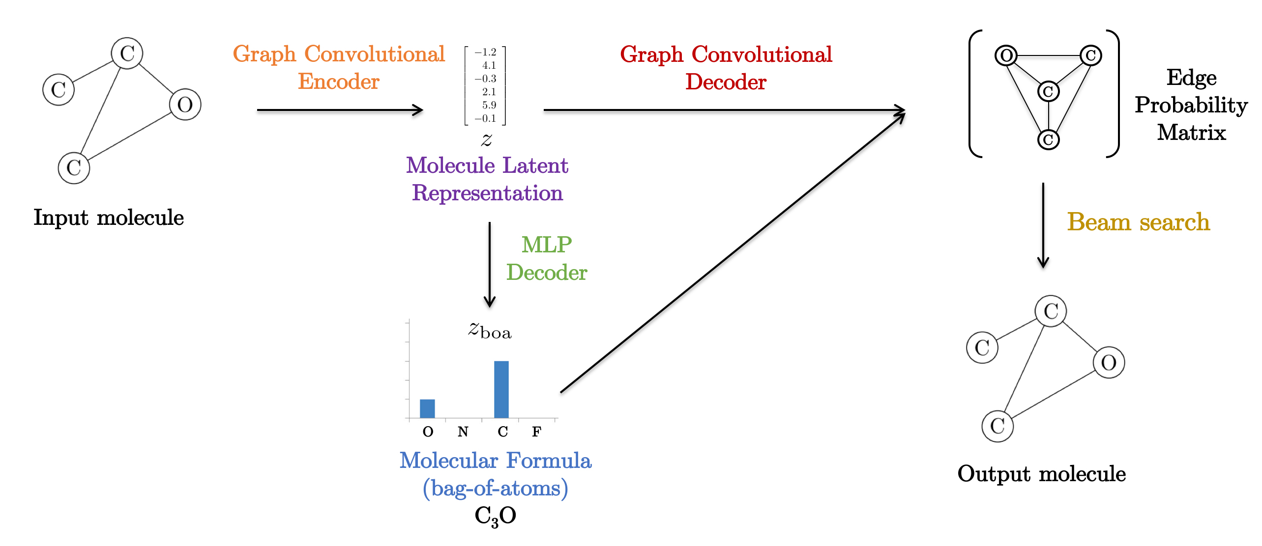
Figure 1: Proposed auto-encoder. The encoder reduces the molecular graph to a latent vector $z$. The decoder uses a MLP to produce a molecular formula and a graph convolutional network classifies each bond between the atoms given by the molecular formula. Finally, a beam search generates a valid molecule.

2.1 Molecule Encoder

For the encoder, each atom type and edge type is first embedded in $\mathbb{R}^{d}$, then these feature are processed by $L$ layers of a graph neural network. We use the graph ConvNet technique introduced in Bresson and Laurent (2018) to compute the hidden node and edge feature representations. Let $h_{i}\in\mathbb{R}^{d}$ and $e_{ij}\in\mathbb{R}^{d}$ denotes the feature vectors on vertex $i$ and edge $(i,j)$ of a graph. If the graph has $N$ vertices, then $h$ is an $N\times d$ matrice, and $e$ is an $N\times N\times d$ tensor. The graph convolutional network will update $h$ and $e$ as follow

$$(h^{\ell+1},e^{\ell+1})=\textrm{GCN}(h^{\ell},e^{\ell})$$ (3)

where

$$h_{i}^{\ell+1} =h_{i}^{\ell}+\textrm{ReLU}\Big{(}\textrm{BN}\Big{(}W_{1}^{\ell}h_{i}^{\ell}+\sum_{j\sim i}\eta_{ij}^{\ell}\odot W_{2}^{\ell}h_{j}^{\ell}\Big{)}\Big{)},$$ (4)

$$e_{ij}^{\ell+1} =e^{\ell}_{ij}+\textrm{ReLU}\Big{(}\textrm{BN}\Big{(}V_{1}^{\ell}e_{ij}^{\ell}+V_{2}^{\ell}h^{\ell}_{i}+V_{3}^{\ell}h^{\ell}_{j}~\Big{)}\Big{)},$$ (5)

and

$$\eta_{ij}^{\ell}=\frac{\sigma(e_{ij}^{\ell})}{\sum_{j^{\prime}\sim i}\sigma(e_{ij^{\prime}}^{\ell})+\varepsilon},$$ (6)

where $\eta_{ij}^{\ell}$ is a dense attention function, $\sigma$ and ReLU denote the standard sigmoid and ReLU non-linearities, and BN stands for batch normalization. We denote by $v\odot w$ the component-wise multiplication between vectors $v$ and $w$. Each layer has a different set of parameters (i.e. the weights are not tied). Finally, a reduction step is applied in order to produces a vector $z$ of fixed size. The graph latent representation is given by the gated sum of edge features:

$$z=\sum_{i,j=1}^{N}\sigma\left(Ae_{ij}^{L}+Bh_{i}^{L}+Ch_{j}^{L}\right)\odot De_{ij}^{L},$$ (7)

where $z\in\mathbb{R}^{k}$ and $k$ is the latent vector dimension. The matrices $A$, $B$, $C$, $D$, $V$ and $W$ are the parameters to be learned.

2.2 Atom generation

The decoder first step is to generate a molecular formula. A molecular formula indicates the numbers of each type of atom in a molecule, with no information on bond structure. For example the molecular formula of carbon dioxide is $\textrm{CO}_{3}$, indicating that this molecule contains one carbon and three oxygens. A molecular formula can be seen as a simple “bag-of-atom” representation of a molecule. Let us assume for the sake of exposition that there are only 3 types of atoms in the set of possible atoms:

$$\mathcal{A}=\{\textrm{C, N, O}\}.$$ (8)

Then the molecular formula of carbon trioxide can be represented by the vector $v=[1,0,3]$ (1 carbon, 0 nitrogen, 3 oxygens). More generally, if we consider molecules with $m$ possible types of atom, the molecular formula can be represented by a vector with $m$ entries that contains the count of each type of atom. Since the molecular formula is represented by a vector of fixed size $m$, it can be easily produced by a fully connected neural network. Hence, the first step of the decoder is to feed the latent vector $z$ to a fully connected neural network, here a one-hidden-layer MLP, to produce a soft molecular formula:

$$z_{\textrm{soft-boa}}=\textrm{MLP}_{\textrm{boa}}(z),$$ (9)

where $z_{\textrm{soft-boa}}$ is a $m\times r$ matrix, where $m$ is the number of atom types and $r$ is the largest possible molecule size in the training set. The molecular formula $z_{\textrm{boa}}\in\mathbb{R}^{m}$ is finally produced by taking the index of the maximum score along the second dimension of $z_{\textrm{soft-boa}}$. Once the molecular formula has been generated, the decoder will decide on how to connect each atom by generating the bonds between the atoms.

2.3 Bond generation

The decoder second step will take the bag-of-atoms vector $z_{\textrm{boa}}$ and the graph latent vector $z$ to assemble the atoms in a single pass. To do this, we start by creating a fully connected graph by connecting each atom in the molecular formula with one another. Each vertex of the fully connected graph receives a feature in $\mathbb{R}^{d}$ corresponding to the atom type via some embedding matrix, and each of the $N^{2}$ edges receives the same embedded feature vector $Uz$, where $z$ is the molecule latent vector, and $U$ is some learnable weight matrix. This fully connected graph is then processed by $L$ layer of the graph convolutional network described by Eq. 3, with new parameters for molecular decoding. The resulting feature vector $e_{ij}^{L}$ of the last convolutional layer can then be used to predict the type of bonds connecting atom $i$ to atom $j$ among possible types in

$$\mathcal{B}=\{\textrm{None, Single, Double, Triple}\},$$ (10)

where a bond type “None” corresponds to a no-bond between atoms. A simple way of predicting the edge type is to use a MLP that classifies each of the vector $e_{ij}^{L}$ independently:

$$s_{ij}=\textrm{MLP}_{\textrm{edge}}(e_{ij}^{L}),$$ (11)

where $s_{ij}\in\mathbb{R}^{n}$ is an edge score and $n$ is the number of bonds in $\mathcal{B}$. The edge type is eventually selected by taking the index of the maximum edge score. We will introduce a more sophisticated beam search strategy for edge type selection that leads to better results.

2.4 Breaking the symmetry

Consider the fully connected graph depicted in the top-right of Figure 1. At initialization, each of the 5 edges of the bond decoder has the exact same feature $Wz$, and each of the 3 carbon atoms has the same feature vector (the embedding vector of the carbon type). When this graph will be processed by the GCN, the features on the carbon atoms will not be able to differentiate from one another (as well as the features on the 3 edges connecting each carbon to the oxygen). In order to remedy to this symmetry problem, we introduce some positional features which allow to embed atoms of the same type into different vectors, and thus differentiate atoms of the same type.

Positional features. Consider the chemical compound dichlorine hexoxide which has molecular formula $\textrm{Cl}_{2}\textrm{O}_{6}$ (2 chlorines and 6 oxygens). Let assume that we have a natural way to order the atoms in the molecule so that the 8 atoms composing dichlorine hexoxide can be written as

$$(\textrm{Cl},1)\;\;\;\;(\textrm{Cl},2)\;\;\;\;(\textrm{O},1)\;\;\;\;(\textrm{O},2)\;\;\;\;(\textrm{O},3)\;\;\;\;(\textrm{O},4)\;\;\;\;(\textrm{O},5)\;\;\;\;(\textrm{O},6)$$ (12)

where $(\textrm{O},3)$, for example, means “$3^{\textrm{rd}}$ oxygen in the molecule". We refer to the number 3 in this example as the “positional feature". It allows us to distinguish this specific oxygen atom from the 5 other oxygen atoms. In order to obtain positional features, we need a consistent way to order the atoms appearing in a molecule (to be more precise, we need a consistent way to rank atoms compared to other atoms of the same type). In this work we simply order the atoms according to the position in which they appear in the canonical SMILES representation of the molecule (a SMILES is a single line text representation of a molecule). To take an example, the notation $(\textrm{O},3)$ in (12), means that this oxygen atom is the third one appearing in the SMILES representation of the dichlorine hexoxide compound. It is important to note that these position features contain some weak structural information about the molecule (this is a consequence of the algorithm that is used to compute a canonical SMILES). For example two carbon atoms $(\textrm{C},4)$ and $(\textrm{C},5)$ are very likely connected to each other. A carbon atom $(\textrm{C},1)$ is very likely at the beginning of a carbon chain.

Using both atom type and positional feature allow us to build better embeddings for the atoms. Let $M$ be an upper bond on the number of atoms contained in the molecule of interest, and let $m$ be the number of different types of atom. To obtain an embedding of $(\textrm{O},3)$, the “$3^{\textrm{rd}}$ oxygen in the molecule", we first concatenate a one-hot-vector in $\mathbb{R}^{m}$ representing O and a one-hot-vector in $\mathbb{R}^{M}$ representing the position feature 3. The resulting vector, which is in $\mathbb{R}^{M+m}$, is then multiplied by a $d$-by-($M+m$) matrix in order to obtain an embedding in $\mathbb{R}^{d}$.

2.5 Variational Auto-Encoder

Finally, we use a VAE formulation in Kingma and Welling (2013) to improve the molecule generation task by “filling” the latent spac. The VAE requires to learn a parametrization of the molecular latent vector $z$ as

$$z=\mu+\sigma\odot\varepsilon,\quad\varepsilon\in\mathcal{N}(0,I),$$ (13)

where $\mu,\sigma$ are learned by the encoder with a reduction layer:

$$f =\sum_{i,j=1}^{N}\sigma\left(A_{f}e_{ij}^{L}+B_{f}h_{i}^{L}+C_{f}h_{j}^{L}\right)\odot D_{f}e_{ij}^{L}\quad\textrm{ for }\quad f=\mu,\sigma.$$ (14)

The total loss is composed of three terms, the cross-entropy loss for edge probability, the cross-entropy loss for bag-of-atoms probability, and the Kullback–Leibler divergence for the VAE Gaussian distribution:

$$L=\lambda_{e}\sum_{ij}\hat{p}_{ij}\log p_{ij}+\lambda_{a}\sum_{i}\hat{q}_{i}\log q_{i}-\lambda_{\textrm{VAE}}\sum_{k}~(1+\log\sigma_{k}^{2}-\mu_{k}^{2}-\sigma_{k}^{2}).$$ (15)

Finally, no matching between input and output molecules is necessary because the same atom ordering is used (with the SMILES representation).

2.6 Beam search

The proposed one-shot decoder may not produce a chemically valid molecule because of a potential violation of atom valency. We use a greedy beam search technique to produce a valid molecule. The beam search is defined as follows. We start with a random edge. We select the next edge that (1) has the largest probability (or by Bernouilli sampling), (2) is connected to the selected edges, and (3) does not violate valency. When the edge selection ends then one molecule is generated. We repeat this process for a number $N_{b}$ of different random initializations, generating $N_{b}$ candidate molecules. Finally, we select the molecule that maximizes the product of edge probabilities or the chemical property to be optimized s.a. druglikeness, constrained solubility, etc.

3 Experiments

Our experimental setup follows the work of Jin et al. (2018).

Molecule dataset. We use the ZINC molecule dataset Irwin et al. (2012), which has 250k drug-like molecules, with up to 38 heavy atoms (excluded Hydrogen). The dataset is originally coded with SMILES. We use the open-source cheminformatics package Rdkit to obtain canonical SMILES representation.

Training. We trained the auto-encoder with mini-batches of 50 molecules of same size. The learning rate is decreased by 1.25 after each epoch if the training loss does not decrease by 1%. The optimization process stops when the learning rate is less than $10^{-6}$. The average training time is 28 hours on one Nvidia 1080Ti GPU.

Molecule reconstruction, novelty and uniqueness. The first task is to reconstruct and sample molecules from the latent space. Table 1 reports the reconstruction and valididty results. We improve the previous state-of-the-art reconstruction accuracy from 76.7% to 90.5% of Jin et al. (2018), with 100% validity (no violation of atom valency) even for the molecules that were not correctly reconstructed. This is an improvement of almost 14% upon previous works. We do not report the reconstruction value for the GAN approach of You et al. (2018), as a GAN is not designed to auto-encode. To evaluate the novelty and uniqueness of the system, we sample 5000 molecules from the latent space from the prior distribution $\mathcal{N}(0,I)$ as in Jin et al. (2018). Table 2 presents the result. Our system does not simply memorize the training set, it is also able to generate 100% of new valid molecules. Besides, all novel molecules are distinct to each other as the novelty measure is 100% (percentage of molecules that are unique in the generated dataset). Figure 2 presents a few generated molecules.

Method	Reconstruction	Validity
CVAE, Gómez-Bombarelli et al. (2018)	44.6%	0.7%
GVAE, Kusner et al. (2017)	53.7%	7.2%
SD-VAE, Dai et al. (2018)	76.2%	43.5%
GraphVAE, Simonovsky and Komodakis (2018)	-	13.5%
JT-VAE, Jin et al. (2018)	76.7%	100.0%
GCPN, You et al. (2018)	-	-
OURS	90.5%	100.0%

Table 1: Encoding and decoding of the 250k ZINC molecules.

Method	Novelty	Uniqueness
JT-VAE, Simonovsky and Komodakis (2018)	100.0%	100.0%
GCPN, You et al. (2018)	-	-
OURS	100.0%	100.0%

Table 2: Sample 5000 molecules from prior distribution.

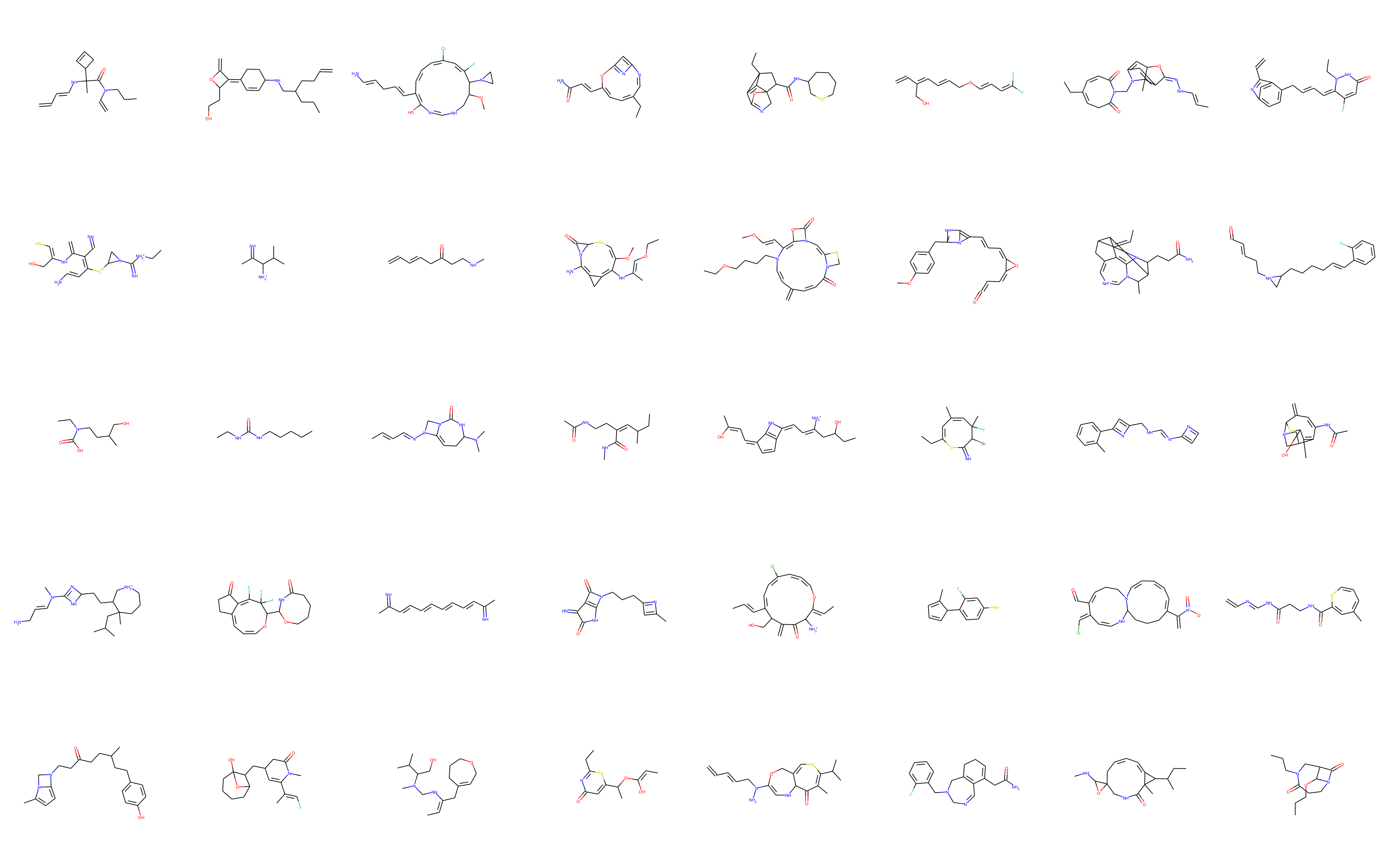
Figure 2: Generated molecules sampled from $\mathcal{N}(0,I)$.

Property Optimization. The second task is to produce new molecules with optimized desired chemical property. We follow the experiment of Jin et al. (2018); Kusner et al. (2017) and select the target property to be the octanol-water partition coefficients (logP) penalized by the synthetic accessibility (SA) score and number of long cycles. To perform the molecular optimization, we train our VAE to simultaneously auto-encode the training molecule and the target chemical property. For this, we add a MLP layer after the graph convolutional encoder to predict the chemical property and a L2 regression loss that penalizes bad property prediction.

We perform gradient ascent w.r.t. the chemical property to optimize in the latent space, then decode the molecule and compute the target property. We optimize the molecules that have the top 100 property values in the training set. Table 3 reports the top-3 molecules from our model and the literature. Our VAE model does slightly better in average, 5.14 vs. 4.90, than the previous state-of-the-art VAE model of Jin et al. (2018). However, the RL model of You et al. (2018) does significantly better than all VAE techniques with a mean value of 7.88. This is expected as RL approaches can extrapolate new data that can be outside the statistics of the training set, whereas VAE approaches can only interpolate data inside the training statistics. Figure 3 presents the top-3 optimized molecules.

Method	1st	2nd	3rd	Mean
ZINC	4.52	4.30	4.23	4.35
CVAE, Gómez-Bombarelli et al. (2018)	1.98	1.42	1.19	1.53
GVAE, Kusner et al. (2017)	2.94	2.89	2.80	2.87
SD-VAE, Dai et al. (2018)	4.04	3.50	2.96	3.50
JT-VAE, Jin et al. (2018)	5.30	4.93	4.49	4.90
OURS (VAE+SL)	5.24	5.10	5.06	5.14
GCPN (GAN+RL), You et al. (2018)	7.98	7.85	7.80	7.88

Table 3: Generative performance of the top three molecules for Penalized logP (logP-SA-Cycle) trained on VAE+SL and GAN+RL.

Figure 3: Generated top-3 molecules. (a) Jin et al. (2018), (b) Ours and (c) You et al. (2018).

Constrained Property Optimization. The third task is to generate novel molecules with optimized chemical property while also constraining molecular similarity between the original molecule and the generated molecule. This is important when we want to optimize the property of a promising molecule in drug discovery and materials science. We follow again the experiment setup of Jin et al. (2018); Kusner et al. (2017). The goal is to maximize the constrained solubility of the 800 test molecules with the lowest property value. We report in Table 4 the property improvements w.r.t. the molecule similarity $\delta$ between the original molecule and the generated molecule. Our model outperform the previous state-of-the-art VAE model of Jin et al. (2018) and the RL model of You et al. (2018) for the property improvement. The RL model outperforms all VAE models for the success rate (a model is successful when it is able to generate a new molecule with the given molecular distance $\delta$). Figure 4 presents constrained optimized molecules w.r.t. the molecular distance.

	JT-VAE, Jin et al. (2018) (VAE+SL)				GCPN, You et al. (2018) (GAN+RL)				OURS (VAE+SL)
$\delta$	Improvement	Similarity	Success		Improvement	Similarity	Success		Improvement	Similarity	Success
0.0	1.91 $\pm$ 2.04	0.28 $\pm$ 0.15	97.5%		4.20 $\pm$ 1.28	0.32 $\pm$ 0.12	100.0%		5.24 $\pm$ 1.55	0.18 $\pm$ 0.12	100.0%
0.2	1.68 $\pm$ 1.85	0.33 $\pm$ 0.13	97.1%		4.12 $\pm$ 1.19	0.34 $\pm$ 0.11	100.0%		4.29 $\pm$ 1.57	0.31 $\pm$ 0.12	98.6%
0.4	0.84 $\pm$ 1.45	0.51 $\pm$ 0.10	83.6%		2.49 $\pm$ 1.30	0.47 $\pm$ 0.08	100.0%		3.05 $\pm$ 1.46	0.51 $\pm$ 0.10	84.0%
0.6	0.21 $\pm$ 0.71	0.69 $\pm$ 0.06	46.4%		0.79 $\pm$ 0.63	0.68 $\pm$ 0.08	100.0%		2.46 $\pm$ 1.27	0.67 $\pm$ 0.05	40.1%

Table 4: Molecular optimization with constrained distances.

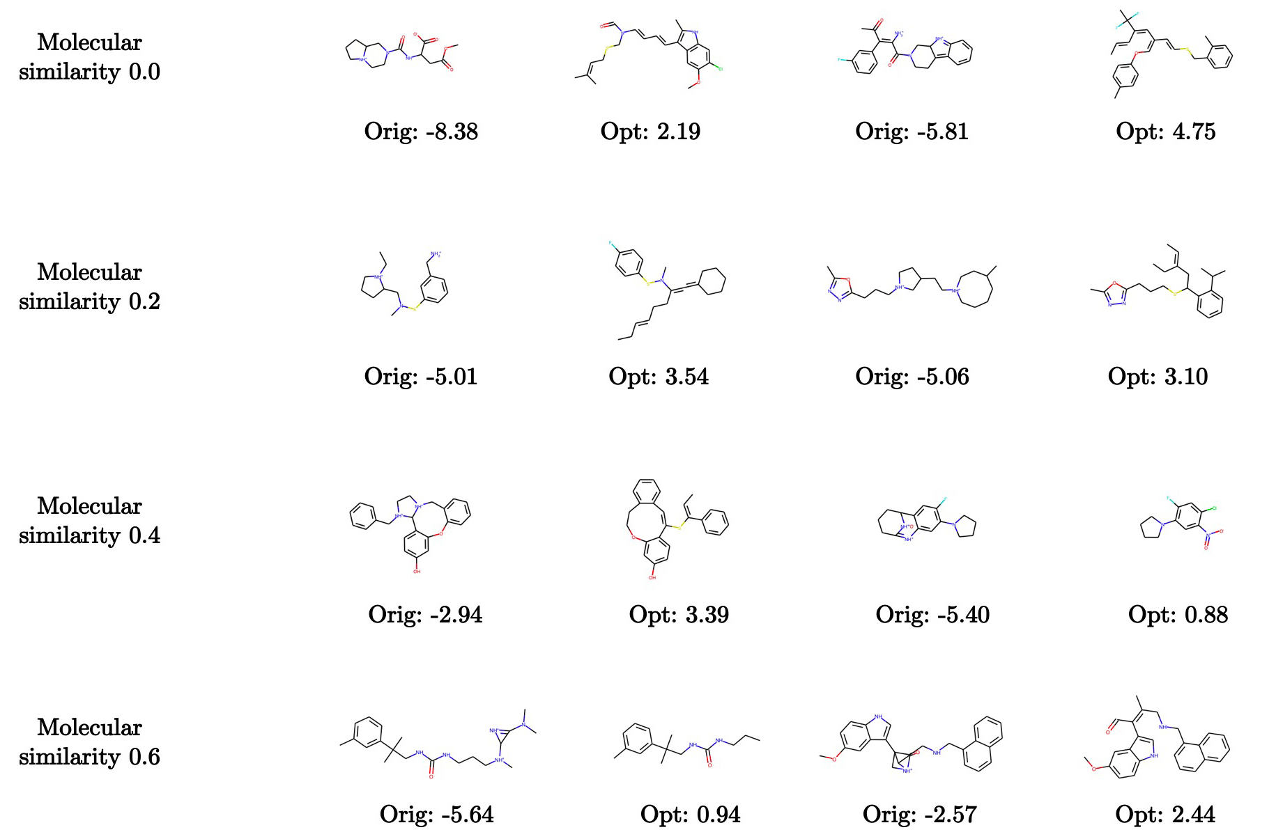
Figure 4: Molecule modification that yields to chemical improvement constrained by molecular similarity. “Orig” means original molecule and “Opt” means optimized molecule.

4 Conclusion

We introduce a simple and efficient VAE model for the molecule generation task. Our decoder generates the molecular formula and the bond structure in one-shot, which can be a faster alternative to autoregressive models. To the best of our knowledge, this is also the first time that beam search is used for improving the molecule generation task. This is also attractive as beam search can be highly parallelized, as for natural language processing systems. Overall, the proposed technique is simpler to implement w.r.t. previous autoregressive VAE techniques such as Jin et al. (2018), which make use of chemical handcrafted features such as ring and tree structure or a molecular grammar in Kusner et al. (2017). We report the highest reconstruction rate for the ZINC dataset. We do not beat the RL technique of You et al. (2018) for optimizing absolute molecular property, but we report the best property improvement results when the optimization is constrained by the distances between the original molecule and the new optimized one. This demonstrates that the proposed VAE is able to learn a good latent space representation of molecules. Future work will explore a RL formulation of the proposed non-autoregressive technique.

5 Acknowledgement

Xavier Bresson is supported in part by NRF Fellowship NRFF2017-10.

References

- Bresson and Laurent [2018] Xavier Bresson and Thomas Laurent. Residual gated graph convnets. International Conference on Learning Representations, 2018.
- Dai et al. [2018] Hanjun Dai, Yingtao Tian, Bo Dai, Steven Skiena, and Le Song. Syntax-directed variational autoencoder for structured data. arXiv preprint arXiv:1802.08786, 2018.
- De Cao and Kipf [2018] Nicola De Cao and Thomas Kipf. Molgan: An implicit generative model for small molecular graphs. arXiv preprint arXiv:1805.11973, 2018.
- Duvenaud et al. [2015] David K Duvenaud, Dougal Maclaurin, Jorge Iparraguirre, Rafael Bombarell, Timothy Hirzel, Alán Aspuru-Guzik, and Ryan P Adams. Convolutional networks on graphs for learning molecular fingerprints. In Advances in neural information processing systems, pages 2224–2232, 2015.
- Gilmer et al. [2017] Justin Gilmer, Samuel S Schoenholz, Patrick F Riley, Oriol Vinyals, and George E Dahl. Neural message passing for quantum chemistry. In International Conference on Machine Learning, 2017.
- Gómez-Bombarelli et al. [2018] Rafael Gómez-Bombarelli, Jennifer N Wei, David Duvenaud, José Miguel Hernández-Lobato, Benjamín Sánchez-Lengeling, Dennis Sheberla, Jorge Aguilera-Iparraguirre, Timothy D Hirzel, Ryan P Adams, and Alán Aspuru-Guzik. Automatic chemical design using a data-driven continuous representation of molecules. ACS central science, 4(2):268–276, 2018.
- Hamilton et al. [2017] Will Hamilton, Zhitao Ying, and Jure Leskovec. Inductive representation learning on large graphs. In Advances in Neural Information Processing Systems, pages 1024–1034, 2017.
- Irwin et al. [2012] John J Irwin, Teague Sterling, Michael M Mysinger, Erin S Bolstad, and Ryan G Coleman. Zinc: a free tool to discover chemistry for biology. Journal of chemical information and modeling, 52(7):1757–1768, 2012.
- Jin et al. [2018] Wengong Jin, Regina Barzilay, and Tommi Jaakkola. Junction tree variational autoencoder for molecular graph generation. arXiv preprint arXiv:1802.04364, 2018.
- Kingma and Welling [2013] Diederik P Kingma and Max Welling. Auto-encoding variational bayes. arXiv preprint arXiv:1312.6114, 2013.
- Kipf and Welling [2017] Thomas N Kipf and Max Welling. Semi-supervised classification with graph convolutional networks. In International conference on Learning Representation, 2017.
- Kusner et al. [2017] Matt J Kusner, Brooks Paige, and José Miguel Hernández-Lobato. Grammar variational autoencoder. In Proceedings of the 34th International Conference on Machine Learning-Volume 70, pages 1945–1954. JMLR, 2017.
- Li et al. [2015] Yujia Li, Daniel Tarlow, Marc Brockschmidt, and Richard Zemel. Gated graph sequence neural networks. arXiv preprint arXiv:1511.05493, 2015.
- Li et al. [2018] Yujia Li, Oriol Vinyals, Chris Dyer, Razvan Pascanu, and Peter Battaglia. Learning deep generative models of graphs. arXiv preprint arXiv:1803.03324, 2018.
- Monti et al. [2017] Federico Monti, Davide Boscaini, Jonathan Masci, Emanuele Rodolà, Jan Svoboda, and Michael M Bronstein. Geometric deep learning on graphs and manifolds using mixture model cnns. In IEEE Conference on Computer Vision and Pattern Recognition (CVPR), pages 5115–5124, 2017.
- Polishchuk et al. [2013] P. G. Polishchuk, T. I. Madzhidov, and A. Varnek. Estimation of the size of drug-like chemical space based on gdb-17 data. Journal of Computer-Aided Molecular Design, 27(8):675–679, 2013.
- Scarselli et al. [2008] F Scarselli, M Gori, AC Tsoi, M Hagenbuchner, and G Monfardini. The graph neural network model. IEEE Transactions on Neural Networks, 20(1):61–80, 2008.
- Simonovsky and Komodakis [2018] Martin Simonovsky and Nikos Komodakis. Graphvae: Towards generation of small graphs using variational autoencoders. In International Conference on Artificial Neural Networks, pages 412–422. Springer, 2018.
- Sukhbaatar et al. [2016] S. Sukhbaatar, A Szlam, and R. Fergus. Learning Multiagent Communication with Backpropagation. Advances in Neural Information Processing Systems (NIPS), pages 2244–2252, 2016.
- Veličković et al. [2017] Petar Veličković, Guillem Cucurull, Arantxa Casanova, Adriana Romero, Pietro Lio, and Yoshua Bengio. Graph attention networks. arXiv preprint arXiv:1710.10903, 2017.
- You et al. [2018] Jiaxuan You, Bowen Liu, Zhitao Ying, Vijay Pande, and Jure Leskovec. Graph convolutional policy network for goal-directed molecular graph generation. In Advances in Neural Information Processing Systems, pages 6412–6422, 2018.