Point interactions with bias potentials

Abstract

We develop an approach on how to define single-point interactions under the application of external fields. The essential feature relies on an asymptotic method based on the one-point approximation of multi-layered heterostructures that are subject to bias potentials. In this approach , the zero-thickness limit of the transmission matrices of specific structures is analyzed and shown to result in matrices connecting the two-sided boundary conditions of the wave function at the origin. The reflection and transmission amplitudes are computed in terms of these matrix elements as well as biased data. Several one-point interaction models of two- and three-terminal devices are elaborated. The typical transistor in the semiconductor physics is modeled in the “squeezed limit” as a $\delta$- and a $\delta^{\prime}$-potential and referred to as a “point” transistor. The basic property of these one-point interaction models is the existence of several extremely sharp peaks as an applied voltage tunes, at which the transmission amplitude is non-zero, while beyond these resonance values, the heterostructure behaves as a fully reflecting wall. The location of these peaks referred to as a “resonance set” is shown to depend on both system parameters and applied voltages. An interesting effect of resonant transmission through a $\delta$-like barrier under the presence of an adjacent well is observed. This transmission occurs at a countable set of the well depth values.

1 Introduction

One-dimensional quantum systems modeled by Schrödinger operators with singular zero-range potentials have been discussed widely in both the physical and mathematical literature (see books [1, 2, 3] for details and references). Additionally, a whole body of literature beginning from the early publications [4, 5, 6, 7, 8, 9, 10, 11] (to mention just a few) has been published, where the one-dimensional stationary Schrödinger equation

$$-\,\psi^{\prime\prime}(x)+V(x)\psi(x)=E\psi(x),$$ (1)

with the potential $V(x)$ given in the form of distributions, where $\psi(x)$ is the wave function and $E$ the energy of an electron, was shown to exhibit a number of peculiar features with possible applications to quantum physics. Currently, because of the rapid progress in fabricating nanoscale quantum devices, of particular importance is the point modeling of different structures like quantum waveguides [12, 13], spectral filters [14, 15] or infinitesimally thin sheets [16, 17].

In the present paper we follow the traditional approach (see the work [7] by Albeverio et al and references therein), according to which there exists a one-to-one correspondence between the full set of self-adjoint extensions of the one-dimensional free Schrödinger operator and the two families of boundary conditions: non-separated and separated. The non-separated extensions describe non-trivial four-parameter point interactions subject to the two-sided at $x=\pm 0$ boundary conditions on the wave function $\psi(x)$ and its derivative $\psi^{\prime}(x)$ given by the connection matrix of the form

$$\left(\begin{array}[]{cc}\psi(+0)\\ \psi^{\prime}(+0)\end{array}\right)=\Lambda\left(\begin{array}[]{cc}\psi(-0)\\ \psi^{\prime}(-0)\end{array}\right),~{}~{}~{}~{}\Lambda={\rm e}^{{\rm i}\chi}\left(\begin{array}[]{cc}\lambda_{11}~{}~{}\lambda_{12}\\ \lambda_{21}~{}~{}\lambda_{22}\end{array}\right),$$ (8)

where $\chi\in[0,\,\pi),~{}\lambda_{ij}\in{\mathbb{R}}$ fulfilling the condition $\lambda_{11}\lambda_{22}-\lambda_{12}\lambda_{21}=1$. The separated point interactions are described by the direct sum of the free Schrödinger operators defined on the half-lines $(-\infty,\,0)$, $(0,\,\infty)$ and subject to the following pair of boundary conditions:

$$\psi^{\prime}(-0)=h^{-}\psi(-0)~{}~{}~{}~{}\mbox{and}~{}~{}~{}~{}\psi^{\prime}(+0)=h^{+}\psi(+0),$$ (9)

where $h^{\pm}\in{\mathbb{R}}\cup\{\infty\}$. For instance, if $\{h^{-},\,h^{+}\}=\{\infty,\,\infty\}$, Equations (9) describe the Dirichlet boundary conditions $\psi(\pm\,0)=0$. In physical terms, a separated self-adjoint extension means that the corresponding point potential is completely opaque for an incident particle. Alternatively, the boundary conditions can be connected using the Asorey-Ibort-Marmo formalism [18] or the Cheon-Fülöp-Tsutsui approach [19, 20]. The advantage of both these connecting representations is that they enable to include all the self-adjoint extensions without treating the particular cases as any parameters tend to infinity. In other words, the relations (9) are excluded from the consideration.

Some particular examples of Equation (1) and the corresponding $\Lambda$-matrix (8) are important in applications. The most simple and widespread potential is Dirac’s delta function $\delta(x)$, i.e., $V(x)=\alpha\delta(x)$ where $\alpha$ is a strength constant (or intensity). The wave function $\psi(x)$ for this interaction (called the $\delta$-interaction or $\delta$-potential) is continuous at the origin $x=0$, whereas its derivative undergoes a jump, so that the boundary conditions read $\psi(-\,0)=\psi(+\,0)=:\psi(0)$ and $\psi^{\prime}(+\,0)-\psi^{\prime}(-\,0)=\alpha\psi(0)$ yielding the $\Lambda$-matrix in the form

$$\Lambda=\left(\begin{array}[]{cc}1~{}~{}~{}0\\ \alpha~{}~{}~{}1\end{array}\right).$$ (10)

In the simplest case, this point potential is constructed from constant functions defined on a squeezed interval.

The dual point interaction for which the derivative $\psi^{\prime}(x)$ is continuous at the origin, but $\psi(x)$ discontinuous, is called a $\delta^{\prime}$-interaction (the notation adopted in the literature [2]). This point interaction with strength $\beta$ defined by the boundary conditions $\psi^{\prime}(-\,0)=\psi^{\prime}(+\,0)=:\psi^{\prime}(0)$ and $\psi(+\,0)=\psi(-\,0)=\beta\psi^{\prime}(0)$ has the $\Lambda$-matrix of the form

$$\Lambda=\left(\begin{array}[]{cc}1~{}~{}~{}\beta\\ 0~{}~{}~{}1\end{array}\right).$$ (11)

As a particular example of the Cheon-Shigehara approach [21], the $\delta^{\prime}$-interaction can be constructed from the spatially symmetric configuration consisting of three separated $\delta$-potentials having the intensities scaled in a nonlinear way as the distances between the potentials tend to zero. Following this approach, Exner, Neidhardt and Zagrebnov [22] have approximated the $\delta$-potentials by regular functions and realized rigorously the similar one-point limit in the norm resolvent topology. In particular, they have proved that the resulting limit takes place if the distances between the peaks of $\delta$-like regularized potentials tend to zero sufficiently slow relative to shrinking these potentials to the origin. The other aspects of the $\delta^{\prime}$-interaction and its approximations by local and nonlocal potentials have been investigated, for instance, by Albeverio and Nizhnik [23, 24, 25, 26], Fassari and Rinaldi [27] (see also references therein). The $\delta^{\prime}$-interaction can be used together with background potentials. Thus, Albeverio, Fassari and Rinaldi [28] have rigorously defined the self-adjoint Hamiltonian of the harmonic oscillator perturbed by an attractive $\delta^{\prime}$-interaction of strength $\beta$ centered at the origin $x=0$ (the bottom of a confining parabolic potential), explicitly providing its resolvent. In a subsequent publication [29], their study has been extended for the perturbation by a triple of attractive $\delta^{\prime}$-interactions using the Cheon-Shigehara approximation. It is worth mentioning the recent publication [30], where Golovaty has constructed a new approximation to the $\delta^{\prime}$-interaction involving two parameters in the boundary conditions. Here the connection matrix

$$\Lambda=\left(\begin{array}[]{cc}\theta~{}~{}~{}~{}\beta\\ 0~{}~{}~{}\theta^{-1}\end{array}\right)$$ (12)

describes the two-parametric family of point interactions being the generalization of the $\delta^{\prime}$-interaction with $\theta=1$.

It should be emphasized that the term “$\delta^{\prime}$-interaction” is somewhat misleading because the point interaction described by the $\Lambda$-matrix (11) does not correspond to Equation (1) in which the potential part is the derivative of the Dirac delta function in the distributional sense, i.e., $V(x)=\gamma\delta^{\prime}(x)$ with strength $\gamma$. Since the term $\delta^{\prime}(x)\psi(x)$ is not defined for discontinuous $\psi(x)$, Kurasov [5] has developed the distribution theory based on the space of discontinuous at $x=0$ test functions. Within this theory, as a particular example, the point interaction that corresponds to the potential $V(x)=\gamma\delta^{\prime}(x)$ is given by the connection matrix

$$\Lambda=\left(\begin{array}[]{cc}\theta~{}~{}~{}~{}0{}\\ 0~{}~{}~{}\theta^{-1}\end{array}\right),$$ (13)

where $\theta=(2+\gamma)/(2-\gamma)$, $\gamma\in{\mathbb{R}}\setminus\{\pm\,2\}$. Since the term “$\delta^{\prime}$-interaction” is reserved for the case with the connection matrix of the type (11), Brasche and Nizhnik [31] suggested to refer the point interactions described by the matrices of the form (13) even if the element $\theta\neq 1$ does not correspond to the delta prime potential. We will follow this terminology in the present paper.

The Kurasov approach has been followed in many applications (see, e.g., [31, 32, 33, 34, 35, 36, 37, 38]) including more general examples. Thus, in the context of this approach, Gadella et al [32] have shown that Equation (1) with the potential $V(x)=a\delta(x)+b\delta^{\prime}(x)$, $a<0$, $b\in{\mathbb{R}}$, has a bound state and calculated the energy of this state in terms of the parameters $a$ and $b$. A new approach based on the integral form of the Schrödinger equation (1) has been developed by Lange [34, 35] with some revision of Kurasov’s theory. The potential $V(x)=a\delta(x)+b\delta^{\prime}(x)$ has also been used by Gadella and coworkers as a perturbation of some background potential, such as a constant electric field and the harmonic oscillator [33] or the infinite square well [36]. The spectrum of a one-dimensional V-shaped quantum well perturbed by three types of a point impurity as well as three solvable two-dimensional systems (the isotropic harmonic oscillator, a square pyramidal potential and their combination) perturbed by a point interaction centered at the origin has been studied by Fassari et al in the recent papers [39, 40, 41].

On the other hand, as derived in the series of publications [42, 43, 44, 45, 46] for some particular cases and proved rigorously by Golovaty with coworkers [47, 48, 49, 50, 51] in a general case, the potential $V(x)=\gamma\delta^{\prime}(x)$ appears to be partially transparent at some discrete values forming a countable set $\{\gamma_{n}\}$ in the $\gamma$-space. The corresponding $\Lambda$-matrix is diagonal, i.e., of the form (13) where the element $\theta=\{\theta_{n}\}$ takes discrete values that depend on the sequence $\{\gamma_{n}\}$. Except the distribution $\delta^{\prime}(x)$, which is obtained as a limit of regular $\delta^{\prime}$-like functions, the diagonal form of the $\Lambda$-matrix can be realized even if the squeezed limit of regular functions does not exist. Beyond the “resonance” set $\{\gamma_{n}\}$, the $\delta^{\prime}$-potential is fully opaque satisfying the boundary conditions of the type (9). However, this resonant-tunneling behavior contradicts with the $\Lambda$-matrix (13) where the element $\theta$ continuously depends on strength $\gamma$. It is remarkable that this controversy can be resolved using the one-dimensional model for the heterostructure consisting of two or three squeezed parallel homogeneous layers approaching to one point [52, 53]. Here a “splitting” effect of one-point interactions has been described.

As for two-point interactions in one dimension, one should mention the recent studies concerning quantum tunneling times and the associated questions such as, for instance, the Hartman effect and its generalized version (see, e.g., [54, 55, 56, 57, 58] and references therein). Another important aspect regarding the application of double-point potentials is the Casimir effect that arises in the behavior of the vacuum energy between two homogeneous parallel plates. For the interpretation of this effect, Muñoz-Castañeda and coworkers [59, 60, 61, 62, 63, 64, 65] reformulated the theory of self-adjoint extensions of symmetric operators over bounded domains in the framework of quantum field theory. Particularly, they have calculated the vacuum energy and identified which boundary conditions generate attractive or repulsive Casimir forces between the plates. Bordag and Muñoz-Castañeda [66] have calculated the quantum vacuum interaction energy between two kinks of the sine-Gordon equation (for a review on nonlinear localized excitations including topological solitons see, e.g., the work [67]) and shown that this interaction induces an attractive force between the kinks in parallel to the Casimir force between conducting mirrors. A rigorous mathematical model of real metamaterials has been suggested in [68]. The resonant tunneling through double-barrier scatters is still an active area of research for the applications to nanotechnology. In the context of the Cheon-Fülöp-Tsutsui approach [19, 20], the conditions for the parameter space under which the perfect resonant transmission occurs through two point interactions, each of which is described by four parameters, have been found by Konno, Nagasawa and Takahashi [69, 70].

The pioneering studies [71, 72, 73] demonstrated that the resonant transmission through quantum multilayer heterostructures of electronic tunnel systems are of considerable general interest. These structures are not only important in micro- and nanodevices, but their study involves a great deal of basic physics. In recent years it has been realized that the study of the electron transmission through heterostructures can be investigated in the zero-thickness limit approximation materialized when their width shrinks to zero. Within such an approximation it is possible to produce various point interaction models, particularly those as described above which admit exact closed analytic solutions. These models are required to provide relatively simple configurations where an appropriate way of squeezing to the zero-width limit must be compatible with the original real structure. Additionally, as a rule, the nanodevices are subject to electric fields applied externally. In this regard, is of great interest to produce point interaction models with bias potentials. So far no models have been elaborated for such devices using one-point approximation methods.

The present paper is devoted to the investigation of planar heterostructures composed of extremely thin layers separated by small distances in the limit where both the layer thickness and the distance between the layers simultaneously tend to zero. The electron motion in the systems of this type is usually confined in the longitudinal direction (say, along the $x$-axis); the latter is perpendicular to the transverse planes where electronic motion is free. The three-dimensional Schrödinger equation of such a structure can be separated into longitudinal and transverse parts, writing the total electron energy as the sum of the longitudinal and transverse energies: $E_{l}+\hbar^{2}{\bf k}_{t}^{2}/2m^{*}$, where $m^{*}$ is an effective electron mass and ${\bf k}_{t}$ the transverse wave vector; for such additive Hamiltonian the wave function is expressed as a product, i.e. $\psi=\psi_{l}\psi_{t}$. As a result, we arrive at the reduced one-dimensional Schrödinger equation with respect to the longitudinal component of the wave function $\psi_{l}(x)$ and the electron energy $E_{l}$. For brevity of notations, in the following we omit the subscript “$l$” at both $\psi_{l}(x)$ and $E_{l}$. Thus, in the units as $\hbar^{2}/2m^{*}=1$, the one-dimensional stationary Schrödinger equation reduces to the form (1) where $V(x)$ is a potential for electrons. Concerning the dimensions of the longitudinal electron position $x$, the potential $V(x)$ and the electron energy $E$, in the system $\hbar^{2}/2m^{*}=1$ we have $[x]$ = nm and $[V,E]$ = nm^-2. For computations we choose $m^{*}=0.1\,m_{e}$ and in this case, 1 eV = 2.62464 nm^-2.

2 Transmission characteristics of multi-layered structures

This introductory section generalizes the approach described in [74]. We consider the Schrödinger equation (1), where the potential $V(x)$ is an arbitrary piecewise function defined on the interval $(x_{0},x_{N})$ with $N$ subsets $(x_{i-1},x_{i})$, $i=\overline{1,N},~{}N=1,2,\ldots$ . Each $V_{i}(x)$ is a real bounded function defined on this interval, so that we have the set of functions: $V_{1}(x),\ldots,V_{N}(x)$. Next, we express the transmission matrix in terms of the interface values of the linearly independent solutions of the Schrödinger equation.

The solution of the Schrödinger equation across the interval $(x_{i-1},x_{i})$, $\psi_{i}(x)$, will be given as

$$\psi_{i}(x)=C_{i}^{(1)}u_{i}(x)+C_{i}^{(2)}v_{i}(x),~{}~{}\overline{1,N},$$ (14)

where $u_{i}(x)$ and $v_{i}(x)$ are linearly independent solutions on the interval $(x_{i-1},x_{i})$. At the interface $x_{i}$, $i=\overline{1,N-1}$, the particle conservation requires the continuity of the wave function $\psi(x)$, while the momentum conservation demands the continuity of the first derivative of the wave function $\psi^{\prime}(x)$ resulting in the equations

$$\psi_{i}(x_{i})=\psi_{i+1}(x_{i}),~{}~{}\psi^{\prime}_{i}(x_{i})=\psi^{\prime}_{i+1}(x_{i}),~{}~{}i=\overline{1,N-1},$$ (15)

where the prime denotes first derivative with respect to $x$.

2.1 Transmission matrix

Using Equation (14), the boundary conditions (15) can be realized as a system of two linear equations with two unknowns such that

$${\bf M}_{i}(x_{i}){\bf C}_{i}={\bf M}_{i+1}(x_{i}){\bf C}_{i+1},~{}~{}~{}i=\overline{1,N-1},~{}~{}N\geq 2,$$ (16)

where

$${\bf C}_{i}:=\mbox{col}\left(C_{i}^{(1)},C_{i}^{(2)}\right)=\left(\begin{array}[]{cc}C_{i}^{(1)}\\ C_{i}^{(2)}\end{array}\right)~{}~{}\mbox{and}~{}~{}{\bf M}_{i}(x):=\left(\begin{array}[]{cc}u_{i}(x)~{}~{}v_{i}(x)\\ u_{i}^{\prime}(x)~{}~{}v^{\prime}_{i}(x)\end{array}\right)$$ (17)

are Wronskian matrices. Next, using Equations (16), one can connect the column vectors ${\bf C}_{1}$ and ${\bf C}_{N}$ as follows

$${\bf C}_{N} = {\bf M}^{-1}_{N}(x_{N-1}){\bf M}_{N-1}(x_{N-1}){\bf M}^{-1}_{N-1}(x_{N-2})\ldots{\bf M}_{2}(x_{2}){\bf M}^{-1}_{2}(x_{1}){\bf M}_{1}(x_{1}){\bf C}_{1}$$ (18)

$$= {\bf M}^{-1}_{N}(x_{N-1})\Lambda_{N-1}(x_{N-2},x_{N-1})\ldots\Lambda_{2}(x_{1},x_{2}){\bf M}_{1}(x_{1}){\bf C}_{1},~{}~{}N\geq 2,$$

where we have introduced the following matrices:

$$\Lambda_{i}(x_{i-1},x_{i}):={\bf M}_{i}(x_{i}){\bf M}^{-1}_{i}(x_{i-1}),~{}~{}~{}i=\overline{2,N-1},~{}~{}N\geq 3.$$ (19)

Here each matrix $\Lambda_{i}(x_{i-1},x_{i})$ connects the boundary values of the corresponding Wronskian matrix ${\bf M}_{i}(x)$ at $x=x_{i-1}$ and $x=x_{i}$. Yet, it is not obvious that the matrices $\Lambda_{i}$’s are transmission matrices connecting the boundary conditions imposed on the wave functions $\psi_{i}(x)$ at $x=x_{i-1}$ and $x=x_{i}$. To prove this fact, we compute the right-hand matrix product of (19) and obtain

$$\Lambda_{i}(x_{i-1},x_{i})=\left(\begin{array}[]{cc}\lambda_{i,11}~{}~{}\lambda_{i,12}\\ \lambda_{i,21}~{}~{}\lambda_{i,22}\end{array}\right),$$ (20)

where

$$\lambda_{i,11}(x_{i-1},x_{i}) = \left[u_{i}(x_{i})v^{\prime}_{i}(x_{i-1})-u^{\prime}_{i}(x_{i-1})v_{i}(x_{i})\right]/W_{i}\,,$$

$$\lambda_{i,12}(x_{i-1},x_{i}) = \left[u_{i}(x_{i-1})v_{i}(x_{i})-u_{i}(x_{i})v_{i}(x_{i-1})\right]/W_{i}\,,$$

$$\lambda_{i,21}(x_{i-1},x_{i}) = \left[u^{\prime}_{i}(x_{i})v^{\prime}_{i}(x_{i-1})-u^{\prime}_{i}(x_{i-1})v^{\prime}_{i}(x_{i})\right]/W_{i}\,,$$

$$\lambda_{i,22}(x_{i-1},x_{i}) = \left[u_{i}(x_{i-1})v^{\prime}_{i}(x_{i})-u^{\prime}_{i}(x_{i})v_{i}(x_{i-1})\right]/W_{i}\,,$$ (21)

with the Wronskian

$$W_{i}=W_{i}(x_{i-1})=u_{i}(x_{i-1})v^{\prime}_{i}(x_{i-1})-u^{\prime}_{i}(x_{i-1})v_{i}(x_{i-1})$$ (22)

computed at $x=x_{i-1}$, which does not depend on $x$ on the interval $(x_{i-1},x_{i})$. Using Equations (21) and (22), one can check that $\det\Lambda_{i}=1.$

There is an infinite number of the linearly independent solutions $u_{i}(x)$ and $v_{i}(x)$. The representation of the $\Lambda_{i}$-matrix elements can be simplified if we choose these solutions satisfying the initial conditions:

$$u_{i}(x_{i-1})=1,~{}~{}u_{i}^{\prime}(x_{i-1})=0,~{}~{}v_{i}(x_{i-1})=0,~{}~{}v_{i}^{\prime}(x_{i-1})=1.$$ (23)

Inserting thus these conditions into Equations (21) and (22), we get that $W_{i}=1$ and, as a result,

$$\Lambda_{i}(x_{i-1},x_{i})=\left(\begin{array}[]{cc}u_{i}(x_{i})~{}~{}~{}~{}v_{i}(x_{i})\\ u^{\prime}_{i}(x_{i})~{}~{}~{}~{}v^{\prime}_{i}(x_{i})\end{array}\right).$$ (24)

The next step is to compute the product $\Lambda_{i}(x_{i-1},x_{i})\mbox{col}\left(\psi_{i}(x_{i-1}),\psi^{\prime}_{i}(x_{i-1})\right)$. This computation immediately results in $\mbox{col}\left(\psi_{i}(x_{i}),\psi^{\prime}_{i}(x_{i})\right)$, so that we have the matrix relation

$$\left(\begin{array}[]{cc}\psi_{i}(x_{i})\\ \psi^{\prime}_{i}(x_{i})\end{array}\right)=\Lambda_{i}(x_{i-1},x_{i})\left(\begin{array}[]{cc}\psi_{i}(x_{i-1})\\ \psi^{\prime}_{i}(x_{i-1})\end{array}\right),$$ (25)

confirming that Equation (19) indeed defines the transmission matrix $\Lambda_{i}(x_{i-1},x_{i})$ expressed in terms of the matrices ${\bf M}_{i}(x_{i-1})$ and ${\bf M}_{i}(x_{i})$. Thus, each transmission matrix $\Lambda_{i}(x_{i-1},x_{i})$ connects the boundary conditions at $x=x_{i-1}$ and $x=x_{i}$.

Equation (18) that connects the column vectors ${\bf C}_{1}$ and ${\bf C}_{N}$ can be transformed to the equation connecting the boundary conditions at $x=x_{0}$ and $x=x_{N}$. To this end, we define the lateral transmission matrices $\Lambda_{i}(x_{i-1},x_{i})$ with $i=0,N$. Thus, on one side, one can write

$${\bf M}_{1}(x_{1}){\bf C}_{1}=\left(\begin{array}[]{cc}\psi_{1}(x_{1})\\ \psi^{\prime}_{1}(x_{1})\end{array}\right)=\Lambda_{1}(x_{0},x_{1})\left(\begin{array}[]{cc}\psi_{1}(x_{0})\\ \psi^{\prime}_{1}(x_{0})\end{array}\right).$$ (26)

On the other hand, multiplying from the left Equation (18) by ${\bf M}_{N}(x_{N})$ and using that

$${\bf M}_{N}(x_{N}){\bf C}_{N}=\left(\begin{array}[]{cc}\psi_{N}(x_{N})\\ \psi^{\prime}_{N}(x_{N})\end{array}\right),$$ (27)

one finds the relation that connects the boundary conditions at $x=x_{0}$ and $x=x_{N}$:

$$\left(\begin{array}[]{cc}\psi_{N}(x_{N})\\ \psi^{\prime}_{N}(x_{N})\end{array}\right)=\Lambda(x_{0},x_{N})\left(\begin{array}[]{cc}\psi_{1}(x_{0})\\ \psi^{\prime}_{1}(x_{0})\end{array}\right)$$ (28)

with

$$\Lambda(x_{0},x_{N})=\Lambda_{N}(x_{N-1},x_{N})\ldots\Lambda_{1}(x_{0},x_{1}).$$ (29)

Thus, the transmission matrix for each layer defined on the interval $(x_{i-1},x_{i})$ can be computed through the solutions $u_{i}(x)$ and $v_{i}(x)$ and their derivatives taken at the boundaries $x=x_{i-1}$ and $x=x_{i}$, resulting in the elements given by Equations (21) and (22).

2.2 Reflection-transmission coefficients

Consider now the solutions outside the interval $(x_{0},x_{N})$. In the region $x<x_{0}$ and $x>x_{N}$ where the potential is a constant, the wave function is the well-known free particle solution of the Schrödinger equation (1) as follows

$$\psi_{0}(x)=A_{1}\exp[ik_{L}(x-x_{0})]+A_{2}\exp[-ik_{L}(x-x_{0})]$$ (30)

for $x<x_{0}$ and

$$\psi_{N+1}(x)=B_{1}\exp[ik_{R}(x-x_{N})]+B_{2}\exp[-ik_{R}(x-x_{N})]$$ (31)

for $x>x_{N}$, where $k_{L}:=\sqrt{E-V_{L}}$ and $k_{R}:=\sqrt{E-V_{R}}\,$. Then the continuity of the boundary conditions at $x=x_{0}$ and $x=x_{N}$ leads to the following equations:

$$\psi_{0}(x_{0})=\psi_{1}(x_{0}),~{}~{}\psi^{\prime}_{0}(x_{0})=\psi^{\prime}_{1}(x_{0}),$$

$$\psi_{N}(x_{N})=\psi_{N+1}(x_{N}),~{}~{}\psi^{\prime}_{N}(x_{N})=\psi^{\prime}_{N+1}(x_{N}),$$ (32)

which can be represented in the matrix form as follows

$${\bf M}_{L}{\bf A}={\bf M}_{1}(x_{0}){\bf C}_{1},~{}~{}~{}{\bf M}_{N}(x_{N}){\bf C}_{N}={\bf M}_{R}{\bf B},$$ (33)

where ${\bf A}:=\mbox{col}(A_{1},A_{2}),$ ${\bf B}:=\mbox{col}(B_{1},B_{2})$ and

$${\bf M}_{L}:=\left(\begin{array}[]{cc}1~{}~{}~{}~{}~{}~{}~{}~{}1\\ ik_{L}~{}-ik_{L}\end{array}\right)\!,~{}~{}~{}{\bf M}_{R}:=\left(\begin{array}[]{cc}1~{}~{}~{}~{}~{}~{}~{}~{}1\\ ik_{R}~{}-ik_{R}\end{array}\right)\!.$$ (34)

Using these matrix equations in Equation (18), we obtain the following basic equation, which allows us to represent the reflection-transmission coefficients through the elements (21) of the transmission matrix $\Lambda(x_{0},x_{N})$:

$$\Lambda(x_{0},x_{N}){\bf M}_{L}{\bf A}={\bf M}_{R}{\bf B}.$$ (35)

Thus, if there is no incidental particle coming from the right, one can set

$$A_{1}=1,~{}~{}A_{2}=R_{L},~{}~{}B_{1}=T_{L},~{}~{}B_{2}=0,$$ (36)

so that in Equation (35) we have ${\bf A}=\mbox{col}(1,R_{L})$ and ${\bf B}=\mbox{col}(T_{L},0)$. Similarly, if there is no incidental particle from the left, we put

$$A_{1}=0,~{}~{}A_{2}=T_{R},~{}~{}B_{1}=R_{R},~{}~{}B_{2}=1,$$ (37)

hence ${\bf A}=\mbox{col}(0,T_{R})$ and ${\bf B}=\mbox{col}(R_{R},1)$ in (35). Then Equation (34) becomes a set of two linear equations with respect to the pair $\{R_{L},T_{L}\}$ or $\{R_{R},T_{R}\}$. Solving these equations and using the relation $\lambda_{11}\lambda_{22}-\lambda_{12}\lambda_{21}=1$, we find

$$R_{L}=-\,{p+{\rm i}q\over D},~{}~{}T_{L}={2k_{L}/k_{R}\over D},~{}~{}R_{R}={p-{\rm i}q\over D},~{}~{}T_{R}={2\over D},$$ (38)

where

$$p:=\lambda_{11}-(k_{L}/k_{R})\lambda_{22}\,,~{}~{}~{}q:=k_{L}\lambda_{12}+k_{R}^{-1}\lambda_{21}$$ (39)

and

$$D:=\lambda_{11}+(k_{L}/k_{R})\lambda_{22}-{\rm i}(k_{L}\lambda_{12}-k_{R}^{-1}\lambda_{21}).$$ (40)

The current $j(x)=({\rm i}/2)(\psi\partial_{x}\psi^{*}-\psi^{*}\partial_{x}\psi)$ has to be conserved across the transition region $x_{0}\leq x\leq x_{N}\,$. Using the definition of the reflection-transmission coefficients given above, we find the left-to-right current $j_{L}(x_{0})=k_{L}(1-|R_{L}|^{2}),$ $j_{L}(x_{N})=k_{R}|T_{L}|^{2}$ and the right-to-left current $j_{R}(x_{0})=-\,k_{L}|T_{R}|^{2},$ $j_{R}(x_{N})=-\,k_{R}(1-|R_{R}|^{2})$. From the equations $j_{L,R}(x_{0})=j_{L,R}(x_{N})$ we obtain the conservation law for both the directions of the current: ${\cal R}_{L,R}+{\cal T}_{L,R}=1$, where

$${\cal R}_{L}:=|R_{L}|^{2},~{}~{}{\cal T}_{L}:=(k_{R}/k_{L})|T_{L}|^{2},~{}~{}{\cal R}_{R}:=|R_{R}|^{2},~{}~{}{\cal T}_{R}:=(k_{L}/k_{R})|T_{R}|^{2}.$$ (41)

One can derive that $|D|^{2}=4k_{L}/k_{R}+p^{2}+q^{2}$ and, as a result, the reflection-transmission amplitudes can be represented in the form

$${\cal R}_{L,R}={p^{2}+q^{2}\over 4k_{L}/k_{R}+p^{2}+q^{2}}\,,~{}~{}~{}{\cal T}_{L,R}={4k_{L}/k_{R}\over 4k_{L}/k_{R}+p^{2}+q^{2}}\,.$$ (42)

In its turn, the scattering matrix can also be represented in terms of the elements of the transmission matrix $\Lambda$. Indeed, due to Equations (38) and (41), this representation reads

$$S=\left(\begin{array}[]{cc}~{}~{}~{}~{}~{}R_{L}~{}~{}~{}~{}~{}~{}~{}~{}~{}\sqrt{k_{L}/k_{R}}\,T_{R}\\ \sqrt{k_{R}/k_{L}}\,T_{L}~{}~{}~{}~{}~{}~{}~{}~{}~{}R_{R}{}{}{}{}{}\end{array}\right)={1\over D}\left(\begin{array}[]{lr}-\,p-{\rm i}q~{}~{}~{}~{}~{}~{}2\sqrt{k_{L}/k_{R}}\\ 2\sqrt{k_{L}/k_{R}}~{}~{}~{}~{}~{}~{}~{}~{}p-{\rm i}q\end{array}\right),$$ (43)

where $p$, $q$ and $D$ are defined by Equations (39) and (40).

3 Schrödinger equation and transmission matrix for the layer with a linear potential profile

Consider now the particular case of a linear potential profile for the layer defined on the interval $(x_{i-1},x_{i})$. In this case the solutions $u_{i}(x)$ and $v_{i}(x)$ and thus the transmission matrix $\Lambda_{i}(x_{i-1},x_{i})$ can be written explicitly. The Schrödinger equation (1) for the $i$th layer, $i=\overline{1,N}$, can be rewritten as

$$-\psi_{i}^{\prime\prime}(x)+V_{i}(x)\psi_{i}(x)=E\psi_{i}(x),$$ (44)

where the potential $V_{i}(x)$ is a linear function defined on the interval $x_{i-1}<x<x_{i}$ of length $l_{i}:=x_{i}-x_{i-i}$, i.e.,

$$V_{i}(x)=\eta_{i}(x-x_{i})+V_{i}(x_{i}),~{}~{}\eta_{i}:={V_{i}(x_{i})-V_{i}(x_{i-1})\over l_{i}}\,.$$ (45)

These equations can be transformed to the Airy equation

$${d^{2}\psi_{i}(z_{i})\over dz_{i}^{2}}-z_{i}\psi_{i}(z_{i})=0,$$ (46)

by setting $z_{i}(x)=\sigma_{i}(x-s_{i})$, where the constants $\sigma_{i}$ and $s_{i}$ are given by

$$\sigma_{i}=\eta_{i}^{1/3},~{}~{}~{}s_{i}=x_{i}+\eta^{-1}_{i}[E-V_{i}(x_{i})].$$ (47)

According to the general expressions (21), we use the Airy functions of the first and the second order as linearly independent solutions to Equation (46), setting $u_{i}(x)=Ai(z_{i}(x))$ and $v_{i}(x)=Bi(z_{i}(x))$. On the interval $-\infty<z_{i}<\infty$, these solutions are real-valued. The interface (boundary) values of the (dimensionless) function $z_{i}(x)$ at the edges of the $i$th layer, to be used in Equations (21) and (22), are

$$z_{i,i-1}:=z_{i}(x)|_{x=x_{i-1}}=-\,\eta_{i}^{-2/3}k^{2}_{i,i-1}\,,~{}~{}~{}z_{i,i}:=z_{i}(x)|_{x=x_{i}}=-\,\eta_{i}^{-2/3}k^{2}_{i,i}\,,$$ (48)

where

$$k_{i,i-1}:=\sqrt{E-V_{i,i-1}}\,,~{}k_{i,i}:=\sqrt{E-V_{i,i}}\,,~{}V_{i,i-1}:=V_{i}(x_{i-1}),~{}V_{i,i}:=V_{i}(x_{i}).\\$$

The Wronskian with respect to the variable $z$ is $W\{Ai(z),Bi(z)\}=1/\pi$, therefore with respect to $x$, it is $W\{Ai(z_{i}(x)),Bi(z_{i}(x))\}=\sigma_{i}/\pi$. Then the elements of the $\Lambda_{i}$-matrix are

$$\lambda_{i,11}(x_{i-1},x_{i}) = \pi\left[Ai(z_{i,i})Bi^{\prime}(z_{i,i-1})-Ai^{\prime}(z_{i,i-1})Bi(z_{i,i})\right],$$

$$\lambda_{i,12}(x_{i-1},x_{i}) = (\pi/\sigma_{i})\left[Ai(z_{i,i-1})Bi(z_{i,i})-Ai(z_{i,i})Bi(z_{i,i-1})\right],$$

$$\lambda_{i,21}(x_{i-1},x_{i}) = \sigma_{i}\pi\left[Ai^{\prime}(z_{i,i})Bi^{\prime}(z_{i,i-1})-Ai^{\prime}(z_{i,i-1})Bi^{\prime}(z_{i,i})\right],$$

$$\lambda_{i,22}(x_{i-1},x_{i}) = \pi\left[Ai(z_{i,i-1})Bi^{\prime}(z_{i,i})-Ai^{\prime}(z_{i,i})Bi(z_{i,i-1})\right],$$ (49)

where the prime denotes the differentiation with respect to $z$.

In the $\eta_{i}\to 0$ limit as $V_{i}(x_{i-1})\to V_{i}(x_{i})$, we obtain

$$z_{i}(x)\to-\,\sigma_{i}s_{i}=\sigma_{i}\left[-x_{i}-{E-V_{i}(x_{i})\over\sigma_{i}^{3}}\right]\to\sigma_{i}^{-2}\left[V_{i}(x_{i})-E\right],$$ (50)

yielding Equation (44) with a constant profile $V_{i}(x)\equiv V_{i}$. In this limit case, one can choose the linearly independent solutions to Equation (44) as

$$u_{i}(x)=\cos[k_{i}(x-x_{i-1})],~{}v_{i}(x)=k_{i}^{-1}\sin[k_{i}(x-x_{i-1})],~{}k_{i}:=\sqrt{k^{2}-V_{i}}\,,$$ (51)

satisfying the initial conditions (23). Therefore, due to Equations (24) and (51), the $\Lambda_{i}$-matrix becomes

$$\Lambda_{i}(x_{i-1},x_{i})=\left(\begin{array}[]{cc}~{}~{}~{}~{}\cos(k_{i}l_{i})~{}~{}~{}~{}k_{i}^{-1}\sin(k_{i}l_{i})\\ -\,k_{i}\sin(k_{i}l_{i})~{}~{}~{}~{}\cos(k_{i}l_{i})\end{array}\right).$$ (52)

4 Asymptotic representations of the single-layer transmission matrix

Similarly to the previous section, here we also focus on one of the layers and for brevity of notations we replace for while in the above expressions the subscripts $\{i,i-1\}$ and $\{i,i\}$ by “0” and “1”, respectively. Then, according to Equations (48) and (3), we write

$$z_{0}=-\left({l\over V_{1}-V_{0}}\right)^{\!\!2/3}k_{0}^{2},~{}z_{1}=-\left({l\over V_{1}-V_{0}}\right)^{\!\!2/3}k_{1}^{2},~{}\sigma=\left({V_{1}-V_{0}\over l}\right)^{\!\!1/3},$$ (53)

where we have replaced $V_{i,i-1}$, $V_{i,i}$, $k_{i,i-1}$, $k_{i,i}$ by $V_{0}$, $V_{1}$, $k_{0}$, $k_{1}$, respectively. Using next the two asymptotic expressions for the Airy functions and their derivatives known in the limit as $z\to 0$ and $z\to\pm\,\infty$, below we will derive the corresponding asymptotic representations of the elements (49) in the two limits as (i) $z_{0},z_{1}\to 0$ and (ii) $z_{0},z_{1}\to\pm\,\infty$. It is reasonable to assume that everywhere $z_{0}$ and $z_{1}$ are of the same sign. We omit for a while the subscript “$i$” for the matrix $\Lambda_{i}$ and its elements.

4.1 Asymptotic representation of the $\Lambda$-matrix in the limit as $z_{0},z_{1}\to 0$

For the $z_{0},z_{1}\to 0$ limit to be carried out in Equations (49), one can use the series representation of the Airy functions and their first derivatives in the neighborhood of the origin $z=0$. It is sufficient to explore only the two first terms:

$$Ai(z) \to {1\over 3^{2/3}\Gamma(2/3)}-{z\over 3^{1/3}\Gamma(1/3)}+\ldots,$$

$$Ai^{\prime}(z) \to -\,{1\over 3^{1/3}\Gamma(1/3)}+{z^{2}\over 2\cdot 3^{2/3}\Gamma(2/3)}+\ldots,$$

$$Bi(z) \to {1\over 3^{1/6}\Gamma(2/3)}+{3^{1/6}z\over\Gamma(1/3)}+\ldots,$$

$$Bi^{\prime}(z) \to {3^{1/6}\over\Gamma(1/3)}+{z^{2}\over 2\cdot 3^{1/6}\Gamma(2/3)}+\ldots.$$ (54)

As a result of applying these expansion formulae to Equations (49) and using Euler’s reflection formula for the gamma function, $\Gamma(1-z)\Gamma(z)=\pi/\sin(\pi z),~{}z\notin{\mathbb{Z}}$, we get the following asymptotic representation of the $\Lambda$-matrix elements:

$$\lambda_{11} \to 1-z_{0}^{2}z_{1}/2,~{}~{}\lambda_{22}\to 1-z_{0}z_{1}^{2}/2,$$

$$\lambda_{12} \to {z_{1}-z_{0}\over\sigma}=l,~{}~{}\lambda_{21}\to{\sigma\over 2}(z_{1}^{2}-z_{0}^{2})=-\,{l\over 2}(k_{0}^{2}+k_{1}^{2})$$ (55)

as $z_{0},z_{1}\to 0$.

4.2 Asymptotic representation of the $\Lambda$-matrix in the limit as $z_{0},z_{1}\to\pm\,\infty$

In the limit as $z\to-\,\infty$, for the Airy functions and their derivatives we have the following asymptotics:

$$Ai(z)\to{\sin\!\left[{2\over 3}(-z)^{3/2}+\pi/4\right]\over\sqrt{\pi}(-z)^{1/4}},~{}~{}Bi(z)\to{\cos\!\left[{2\over 3}(-z)^{3/2}+\pi/4\right]\over\sqrt{\pi}(-z)^{1/4}},$$ (56)

$$Ai^{\prime}(z) \to {\frac{1}{4}(-z)^{-3/4}\sin\!\left[{2\over 3}(-z)^{3/2}+\pi/4\right]-(-z)^{3/4}\cos\!\left[{2\over 3}(-z)^{3/2}+\pi/4\right]\over\sqrt{\pi}(-z)^{1/2}},~{}~{}$$

$$Bi^{\prime}(z) \to {\frac{1}{4}(-z)^{-3/4}\cos\!\left[{2\over 3}(-z)^{3/2}+\pi/4\right]+(-z)^{3/4}\sin\!\left[{2\over 3}(-z)^{3/2}+\pi/4\right]\over\sqrt{\pi}(-z)^{1/2}}.$$

Using this asymptotic representation in Equations (49) as $z_{0},z_{1}\to-\,\infty$, we obtain

$$\lambda_{11} \to (-z_{0})^{1/4}(-z_{1})^{-1/4}\cos\!\chi_{-}-(4z_{0})^{-1}(-z_{0})^{-1/4}(-z_{1})^{-1/4}\sin\!\chi_{-}\,,$$

$$\lambda_{12} \to -\,\sigma^{-1}(-z_{0})^{-1/4}(-z_{1})^{-1/4}\sin\!\chi_{-}\,,$$

$$\lambda_{21} \to \sigma\,(-z_{0})^{-1/2}(-z_{1})^{-1/2}$$

$$\times\left\{\left[(-z_{0})^{3/4}(-z_{1})^{3/4}+4^{-2}(-z_{0})^{-3/4}(-z_{1})^{-3/4}\right]\sin\!\chi_{-}\right.$$

$$+\left.4^{-1}\left[(-z_{0})^{3/4}(-z_{1})^{-3/4}-(-z_{1})^{3/4}(-z_{0})^{-3/4}\right]\cos\!\chi_{-}\right\},$$

$$\lambda_{22} \to (-z_{1})^{1/4}(-z_{0})^{-1/4}\cos\!\chi_{-}+(4z_{1})^{-1}(-z_{0})^{-1/4}(-z_{1})^{-1/4}\sin\!\chi_{-}\,,~{}~{}~{}~{}~{}~{}$$ (58)

where

$$\chi_{-}:=\frac{2}{3}\!\left[(-z_{1})^{3/2}-(-z_{0})^{3/2}\,\right].$$ (59)

One can check that $\det\Lambda=1$. According to Equations (53), this representation corresponds to a well ($V_{j}<0$, $j=0,1$). However, these formulae can be “continued” to positive values of $z_{0}$ and $z_{1}$ that correspond to a barrier with $E<V_{j}$. To prove this, we use the asymptotic representation of the Airy functions and their derivatives in the limit as $z_{0},z_{1}\to+\,\infty$:

$$Ai(z)\to{{\rm e}^{-\,{2\over 3}z^{3/2}}\over~{}~{}~{}2\sqrt{\pi}z^{1/4}}\,,~{}~{}~{}Bi(z)\to{{\rm e}^{{2\over 3}z^{3/2}}\over\sqrt{\pi}z^{1/4}}\,,$$ (60)

$$Ai^{\prime}(z)\to-\,{z^{3/4}+{1\over 4}z^{-3/4}\over 2\sqrt{\pi}z^{1/2}}\,{\rm e}^{-\,{2\over 3}z^{3/2}},~{}~{}Bi^{\prime}(z)\to{z^{3/4}-{1\over 4}z^{-3/4}\over\sqrt{\pi}z^{1/2}}\,{\rm e}^{{2\over 3}z^{3/2}}$$ (61)

and, as a result, we find

$$\lambda_{11} \to (z_{0}/z_{1})^{1/4}\cosh\!\chi_{+}+(4z_{0})^{-1}(z_{0}z_{1})^{-1/4}\sinh\!\chi_{+}\,,$$

$$\lambda_{12} \to \sigma^{-1}(z_{0}z_{1})^{-1/4}\sinh\!\chi_{+}\,,$$

$$\lambda_{21} \to \sigma\,(z_{0}z_{1})^{-1/2}\left\{\left[(z_{0}z_{1})^{3/4}-4^{-2}(z_{0}z_{1})^{-3/4}\right]\sinh\!\chi_{+}\right.$$

$$~{}~{}~{}~{}~{}+\left.4^{-1}\left[(z_{1}/z_{0})^{3/4}-(z_{0}/z_{1})^{3/4}\right]\cosh\!\chi_{+}\right\},$$

$$\lambda_{22} \to (z_{1}/z_{0})^{1/4}\cosh\!\chi_{+}-(4z_{1})^{-1}(z_{0}z_{1})^{-1/4}\sinh\!\chi_{+}\,,$$ (62)

where $z_{0}$ and $z_{1}$ are positive and

$$\chi_{+}:=\frac{2}{3}\!\left(z_{1}^{3/2}-z_{0}^{3/2}\right).$$ (63)

Similarly, for the elements (62) one can also check that $\det\Lambda=1$. In fact, Equations (62) with (63) appear to coincide with Equations (58) and (59) if we assume that in the latter equations $z_{0}$ and $z_{1}$ are positive. To show this, we note that $(-z)^{3/2}={\rm i}^{3}z^{3/2}=-{\rm i}z^{3/2}$ and, as a result, we get the relation $\chi_{-}=-{\rm i}\chi_{+}$ for positive $z_{0}$ and $z_{1}$ in both Equations (59) and (63). Next, the elements (62) are obtained from the representation (58) if we note that $(-z_{0})^{1/4}(-z_{1})^{1/4}={\rm i}(z_{0}z_{1})^{1/4}$, $(-z_{0})^{1/2}(-z_{1})^{1/2}=-(z_{0}z_{1})^{1/2}$ and $(-z_{0})^{3/4}(-z_{1})^{3/4}=-{\rm i}(z_{0}z_{1})^{3/4}$. Therefore in the following it is sufficient to consider only the representation given by Equations (58) and (59), being valid for both negative and positive $z_{0}$ and $z_{1}$.

Using the explicit values for $z_{0}$ and $z_{1}$ given by Equations (53), the expression (59) for $\chi_{-}$ can be transformed to

$$\chi_{-}=\mbox{sgn}(V_{0}-V_{1})\,k_{1,0}\,l,$$ (64)

where

$$k_{1,0}:={2(k_{0}^{2}+k_{1}^{2}+k_{0}k_{1})\over 3(k_{0}+k_{1})},~{}~{}~{}k_{j}:=\sqrt{E-V_{j}}\,~{}~{}j=0,1.$$ (65)

Inserting next the expressions (53) and (64) into Equations (58), one can write the elements of the $\Lambda$-matrix in terms of $k_{0}$ and $k_{1}$ as follows

$$\lambda_{11} \to \left({k_{0}\over k_{1}}\right)^{\!1/2}\!\cos(\kappa l)+{k_{1}^{2}-k_{0}^{2}\over 4l}k_{0}^{-5/2}k_{1}^{-1/2}\sin(k_{1,0}\,l),$$

$$\lambda_{12} \to k_{0}^{-1/2}k_{1}^{-1/2}\sin(k_{1,0}\,l),$$

$$\lambda_{21} \to {3(k_{0}^{2}-k_{1}^{2})^{2}k_{1,0}\over 8lk_{0}^{5/2}k_{1}^{5/2}}\cos(k_{1,0}\,l)$$

$$-\,k_{0}^{1/2}k_{1}^{1/2}\!\left[1+\left({k_{0}^{2}-k_{1}^{2}\over 4l}\right)^{\!\!2}k_{0}^{-3}k_{1}^{-3}\right]\!\sin(k_{1,0}\,l),$$

$$\lambda_{22} \to \left({k_{1}\over k_{0}}\right)^{\!1/2}\!\cos(\kappa l)+{k_{0}^{2}-k_{1}^{2}\over 4l}k_{0}^{-1/2}k_{1}^{-5/2}\sin(k_{1,0}\,l),$$ (66)

where $k_{1,0}$ is defined by Equation (65). One can check that the matrix elements (66) together with the argument (65) satisfy the condition $\det\Lambda=1$. Note that the only restriction for the existence of the representation (66) are the asymptotics $z_{0},z_{1}\to\pm\,\infty$. Both $k_{0}$ and $k_{1}$ are either real-valued or imaginary. In the particular case $V_{1}=V_{0}$ ($k_{1}=k_{0}$), Equations (65) and (66) reduce to the matrix representation (52).

5 Realization of point interactions in the zero-thickness limit for one layer

Keeping in the following the same notations with respect to the subscripts “0” and “1”, let us consider the linear potential (45) rewritten as

$$V(x)=V_{0}+{V_{1}-V_{0}\over l}\,x,~{}~{}V_{0},\,V_{1}\in{\mathbb{R}},$$ (67)

on the interval $0<x<l$, where $V_{0}$ and $V_{1}$ are the potential values at the left and right edges of the layer with width $l$. Consider first the case when this potential is constant, i.e., $V_{0}=V_{1}$. A point interaction can be realized in the limit as the layer thickness $l\to 0$, whereas $V_{0}\to\pm\,\infty$. To this end, one can use the parametrization of the potential $V(x)\equiv V_{0}$ introducing a dimensionless parameter $\varepsilon>0$ that controls the shrinking of the layer to zero width as $\varepsilon\to 0$. It is natural to consider the power parametrization setting

$$V_{0}=a\,\varepsilon^{-\mu},~{}~{}l=\varepsilon d,~{}~{}a\in{\mathbb{R}},~{}~{}\mu,\,d>0.$$ (68)

Figure 1: Schematics of one-layer potential (67) tilted by difference $V_{1}-V_{0}$ (solid line) with notations given in (69) at $\varepsilon=1$: $V_{1}-V_{0}=b=V_{R}$. The dashed line represents potential with $b=0$.

In the squeezed limit (as $\varepsilon\to 0$), a one-parameter family of point interactions at $x=0$ is realized. It is determined by the power $\mu\in(0,\infty)$: the transmission is perfect for $\mu\in(0,1)$, at $\mu=1$ the potential takes the form of Dirac’s delta function $\alpha\delta(x)$ with the transmission matrix (10), where $\alpha=ad$ is the strength of the $\delta$-interaction, and for $\mu\in(1,\infty)$ the interaction acts as a fully reflecting wall satisfying the Dirichlet boundary condition $\psi(\pm 0)=0$ for the wave function $\psi(x)$.

In the case when the difference $V_{1}-V_{0}$ is non-zero, as shown in Figure 1, one deals with two potential values $V_{0}$ and $V_{1}$ at the layer edges that must tend to infinity in the zero-thickness limit. Both the potential values $V_{0}$ and $V_{1}$ are supposed to be of the same sign. In general, the rate of this divergence to infinity can differ and therefore the parametrization of the potential (67) should involve two parameters. We introduce the two powers $\mu$ and $\nu$, where the parameters $\mu$ and $\nu$ describe how rapidly the potential $V_{0}$ at the left layer edge and the difference $V_{1}-V_{0}$ tend (escape) to infinity as $\varepsilon\to 0$, respectively. The particular case when this difference is a constant not depending on $\varepsilon$ can also be included. Thus, we set

$$V_{0}=a\varepsilon^{-\mu},~{}V_{1}=V_{0}+b\,\varepsilon^{-\nu},~{}0<\mu<\infty,~{}0\leq\nu\leq\mu,~{}a,\,b\in{\mathbb{R}},~{}l=\varepsilon\,d,~{}~{}~{}~{}~{}$$ (69)

including the following two situations in the squeezed limit: (i) $V_{1}-V_{0}$ is constant ($\nu=0$) and (ii) the “escaping-to-infinity” rate of $V_{1}-V_{0}$ does not exceed the rate of $V_{0}$ ($\nu\leq\mu$). In the electronics domain the difference $V_{1}-V_{0}$ or $b$ may play the role of a bias voltage.

Due to Equations (48), we have the asymptotics $z_{0},z_{1}\sim\varepsilon^{2(1+\nu)/3-\mu}$. Consequently, the line $L_{0,\infty}:=\{0<\mu\leq 2,\,\nu=3\mu/2-1\}$ separates the asymptotic representations $z_{0},z_{1}\to 0$ and $z_{0},z_{1}\to\pm\,\infty$ on the ($\mu,\nu$)-plane as illustrated by the diagram depicted in Figure 2.

Figure 2: Regions of asymptotic representations $z_{0},z_{1}\to 0$ ($S_{0}$) and $z_{0},z_{1}\to\pm\,\infty$ ($S_{\infty}$) with separating line $L_{0,\infty}$. Three balls indicate characteristic points $P_{1,1}:=\{\mu=\nu=1\}\in S_{0}\,$, $P_{2,0}:=\{\mu=2,\,\nu=0\}\in S_{\infty}$ and $P_{2,1}:=\{\mu=2,\,\nu=1\}\in S_{\infty}$.

Here, we have the two triangle sets:

$$S_{0} := \{0<\mu<2,\,\max\{0,\,3\mu/2-1\}<\nu\leq\mu\}\cup\{0<\mu<2/3,\,\nu=0\},$$

$$S_{\infty} := \{2/3<\mu\leq 2,\,0\leq\nu<3\mu/2-1\},$$ (70)

where the asymptotic representations $z_{0},z_{1}\to 0$ and $z_{0},z_{1}\to\pm\,\infty$ take place, respectively. The corresponding angles are formed by the boundary lines: $S_{0}$ by $L_{0,1}:=\{0<\mu<2/3,\,\nu=0\}$, $L_{0,2}:=\{0<\mu<2,\,\nu=\mu\}$ and $S_{\infty}$ by $L_{\infty,1}:=\{2/3<\mu\leq 2,\,\nu=0\}$, $L_{\infty,2}:=\{\mu=2,\,0<\nu<2\}$.

5.1 Point interactions realized in the limit as $z_{0},z_{1}\to 0$

Let us consider the boundary lines $L_{0,1}$ and $L_{0,2}$ of the angle $S_{0}$. On the line $L_{0,1}$, we find that $z_{0},z_{1}\sim\varepsilon^{2/3-\mu}$, so that the $z_{0},z_{1}\to 0$ limit takes place on the interval $0<\mu<2/3$. Next, we have $k_{0}^{2},k_{1}^{2}\sim\varepsilon^{-\mu}$ and according to Equations (55), $\lambda_{12}\to 0$ and $\lambda_{21}\sim\varepsilon^{1-\mu}\to 0$, so that the $\Lambda$-matrix becomes the identity ($\Lambda=I$) because $\mu<1$.

Similarly, on the line $L_{0,2}\,$, where $z_{0},z_{1}\sim\varepsilon^{(2-\mu)/3}$, from Equations (53) and (55) we get the asymptotics

$$\lambda_{11} \to 1-\,c_{1}\varepsilon^{2-\mu},~{}~{}\lambda_{12}\to\varepsilon d,$$

$$\lambda_{21} \to (a+b/2)d\,\varepsilon^{1-\mu},~{}~{}\lambda_{22}\to 1-c_{2}\,\varepsilon^{2-\mu}$$ (71)

with

$$c_{1}:=(a^{2}/2)(a+b)(d/b)^{2},~{}~{}c_{2}:=(a/2)(a+b)^{2}(d/b)^{2}.$$ (72)

Therefore, on the interval $0<\mu<1$ the transmission matrix is the identity $I$, while on the interval $1<\mu<2$ the transmission matrix does not exist. In this case the point interaction acts as a fully reflecting wall (the boundary conditions for this point interaction are of the Dirichlet type). The value $\mu=1$ describes the intermediate situation with a partial transmission through the system, namely the $\delta$-interaction with bias $b$, which separates both these regimes. The limit transmission matrix (as $\varepsilon\to 0$) corresponds to the $\delta$-interaction described by the connection matrix (10) with the strength constant

$$\alpha=(a+b/2)d.$$ (73)

This result also includes the constant case when $V_{0}=V_{1}$, i.e., $b=0$. This approximation is appropriate for modeling the $\delta$-potential. Note that similar analysis can be done for $\mu$ and $\nu$ belonging to the interior of $S_{0}$. In this case in the above equations we have to set $b=0$.

Using the second formula (42), one can compute the transmission amplitude for this $\delta$-interaction. We get

$${\cal T}={4k\,k_{R}\over(k+k_{R})^{2}+\alpha^{2}},$$ (74)

where $\alpha$ is given by (73). In the unbiased case ($b=0,~{}k_{R}=k$) this formula reduces to ${\cal T}=\left[1+(\alpha/2k)^{2}\right]^{-1}$ with $\alpha=ad$, the well known expression for the constant potential. Equation (74) has been obtained for any $a\in{\mathbb{R}}$. However, for negative values of $a$, i.e., for a $\delta$-like well, it does not describe the oscillating behavior with respect to the constant $\alpha$ that takes place under tunneling across a well with finite thickness $l$.

5.2 Point interactions realized in the limit as $z_{0},z_{1}\to\pm\,\infty$

Consider now the characteristic point $P_{2,1}\in S_{\infty}$ setting in Equations (66) $\mu=2$ and $\nu=1$. Here $k_{0}^{2}-k_{1}^{2}=V_{1}-V_{0}=b\,\varepsilon^{-1}$ and $k_{0},k_{1},k_{1,0}\to\sqrt{-\,a}\,\varepsilon^{-1}$, so that the asymptotic representation of Equations (66) in the limit as $\varepsilon\to 0$ becomes

$$\lambda_{11} \to \cos(\kappa d)-\varepsilon\,g\sin(\kappa d),$$

$$\lambda_{12} \to \varepsilon\,\kappa^{-1}\sin(\kappa d),$$

$$\lambda_{21} \to -\,\varepsilon^{-1}\kappa\sin(\kappa d)+{\cal O}(\varepsilon),$$

$$\lambda_{22} \to \cos(\kappa d)+\varepsilon\,g\sin(\kappa d),$$ (75)

where

$$\kappa:=\sqrt{-\,a},~{}~{}~{}g:=\kappa^{-3}(b/4d).$$ (76)

As follows from these asymptotic expressions derived at the point $P_{2,1}$, in the limit as $\varepsilon\to 0$, the transmission through a barrier is zero, while across a well ($a<0$) it appears to be resonant. The resonance set consists of the roots of the equation $\sin(\kappa d)=0$. At fixed $d>0$, these roots form the countable set $\Sigma=\cup_{n=0}^{\infty}\sigma_{n}$ formed from the points $\sigma_{n}:=-\,(n\pi/d)^{2}$. On this resonance set, the discrete-valued matrix is $\Lambda_{n}:=\Lambda|_{\Sigma}=(-1)^{n}I$. Beyond these resonance values, the $\delta$-like well is opaque and, instead of the identity matrix $I$, the two-sided boundary conditions for the wave function are of the Dirichlet type ($\psi(\pm\,0)=0$).

6 Multi-layered heterostructures with bias

Now we are ready to apply the expressions obtained above for a single layer to the total structure consisting of an arbitrary number $N$ of layers replacing $\mu\to\mu_{i}\,,~{}\nu\to\nu_{i}\,,~{}b\to b_{i}\,,~{}d\to d_{i}\,.$ Taking for account that the left boundary value for the potential of the $i$th layer $a_{i}$ is shifted because of the biases $b_{1}\,,\ldots b_{i-1}$ in the left-hand layers, we need to use the following replacement rule:

$$a\to a_{i}+\sum_{j=1}^{i-1}b_{j}\,,~{}~{}i=\overline{1,N},$$ (77)

where the sum vanishes if $i=1$. Then Equations (69) are transformed to

$$V_{0}\to V_{i,i-1}=\left(a_{i}+\sum_{j=1}^{i-1}b_{j}\right)\!\varepsilon^{-\mu_{i}},~{}~{}V_{1}\to V_{i,i}=V_{i,i-1}+b_{i}\,\varepsilon^{-\,\nu_{i}}.$$ (78)

Next, all the other expressions derived above should be rewritten for the $i$th layer using the following replacement rules:

$$z_{0} \to z_{i,i-1}=\left({d_{i}\over b_{i}}\right)^{\!\!2/3}\left[\left(a_{i}+\sum_{j=1}^{i-1}b_{j}\right)\!\varepsilon^{-\mu_{i}}-E\right]\!\varepsilon^{2(1+\nu_{i})/3},$$

$$z_{1} \to z_{i,i}=\left({d_{i}\over b_{i}}\right)^{\!\!2/3}\left[\left(a_{i}+\sum_{j=1}^{i-1}b_{j}\right)\!\varepsilon^{-\mu_{i}}+b_{i}\,\varepsilon^{-\nu_{i}}-E\right]\!\varepsilon^{2(1+\nu_{i})/3},$$

$$\alpha \to \alpha_{i}=\left(a_{i}+\sum_{j=1}^{i-1}b_{j}+b_{i}/2\right)\!d_{i}\,,~{}~{}\sigma\to\sigma_{i}=\left(b_{i}\over d_{i}\right)^{\!\!\!1/3}\!\!\varepsilon^{-(1+\nu_{i})/3},$$

$$\kappa \to \kappa_{i}=\sqrt{-\left(a_{i}+\sum_{j=1}^{i-1}b_{j}\right)},~{}~{}g\to g_{i}={b_{i}\over 4\kappa_{i}^{3}d_{i}}\,,$$

$$c_{1} \to c_{i,1}=\frac{1}{2}\left(a_{i}+\sum_{j=1}^{i-1}b_{j}\right)^{\!\!\!2}\left(a_{i}+\sum_{j=1}^{i}b_{j}\right)\left({d_{i}\over b_{i}}\right)^{\!\!2},$$

$$c_{2} \to c_{i,2}=\frac{1}{2}\left(a_{i}+\sum_{j=1}^{i-1}b_{j}\right)\left(a_{i}+\sum_{j=1}^{i}b_{j}\right)^{\!\!\!2}\left({d_{i}\over b_{i}}\right)^{\!\!2}.$$ (79)

In the following we will consider some particular examples of multi-layered structures with $N=2,3$. It will be shown that in some cases two- and three-lateral quantum devices can be approximated by one-point interactions.

6.1 Two-layered structures

Consider now the structure consisting of two layers ($N=2$). The piecewise linear potential of a barrier-well form is shown in Figure 3.

Figure 3: Schematics of tilted (solid line) and piecewise constant (dashed line) barrier-well potential, where notations correspond to Equations (77) and (78) for $N=2$ and $\varepsilon=1$. Potential values at layer edges are $V_{1,0}=a_{1}$, $V_{1,1}=a_{1}+b_{1}$ (barrier, $a_{1}>0$) and $V_{2,1}=a_{2}+b_{1}$, $V_{2,2}=a_{2}+b_{1}+b_{2}$ (well, $a_{2}<0$). Polarity is shown positive (left-to-right electron flow, $b_{1}\,,b_{2}<0$). Dashed lines show unbiased potential ($b_{1}=b_{2}=0$).

For an arbitrary two-layered structure, the limit transmission matrix is the product $\Lambda=\Lambda_{2}\Lambda_{1}$, where the matrices $\Lambda_{i}$’s can be constructed from the asymptotic approximations (71) and (75) by applying the replacement rules (77)-(79). Applying these rules in Equations (71), (72) and (75), (76) to the matrices $\Lambda_{1}$ and $\Lambda_{2}$, below we compute their product for two different situations. Note that due to the presence of the factor $\varepsilon^{-1}$ in the expression $\lambda_{21}$ [see Equations (75)], the terms of order ${\cal O}(\varepsilon)$ must be kept in the product $\Lambda_{2}\Lambda_{1}$ because $\lim_{\varepsilon\to 0}\Lambda_{2}\cdot\lim_{\varepsilon\to 0}\Lambda_{1}\neq\lim_{\varepsilon\to 0}(\Lambda_{2}\Lambda_{1})$.

Point interactions of a $\delta^{\prime}$-type: Consider the zero-thickness limit determined by the powers $\mu_{1}=\mu_{2}=2$ and $\nu_{1}=\nu_{2}=1$. Then, the product $\Lambda=\Lambda_{2}\Lambda_{1}$ yields the following asymptotic representation of the $\Lambda$-matrix elements for the total double-layer system:

$$\lambda_{11} \to \cos(\kappa_{1}d_{1})\cos(\kappa_{2}d_{2})-(\kappa_{1}/\kappa_{2})\sin(\kappa_{1}d_{1})\sin(\kappa_{2}d_{2}),$$

$$\lambda_{12} \to 0,$$

$$\lambda_{21} \to \alpha-\,\varepsilon^{-1}\left[\kappa_{1}\sin(\kappa_{1}d_{1})\cos(\kappa_{2}d_{2})+\kappa_{2}\cos(\kappa_{1}d_{1})\sin(\kappa_{2}d_{2})\right],$$

$$\lambda_{22} = \cos(\kappa_{1}d_{1})\cos(\kappa_{2}d_{2})-\,(\kappa_{2}/\kappa_{1})\sin(\kappa_{1}d_{1})\sin(\kappa_{2}d_{2}),$$ (80)

where the $\varepsilon\to 0$ limit has been performed and

$$\alpha=(\kappa_{2}g_{1}-\kappa_{1}g_{2})\sin(\kappa_{1}d_{1})\sin(\kappa_{2}d_{2}).$$ (81)

The second term in the element $\lambda_{21}$ diverges as $\varepsilon\to 0$ and it vanishes if the equation

$$\kappa_{1}\tan(\kappa_{1}d_{1})+\kappa_{2}\tan(\kappa_{2}d_{2})=0$$ (82)

takes place. Using this equation in the elements $\lambda_{11}$ and $\lambda_{22}$ [see Equations (80)], we find the total transmission matrix

$$\Lambda=\left(\begin{array}[]{ll}\cos(\kappa_{1}d_{1})/\cos(\kappa_{2}d_{2})~{}~{}~{}~{}~{}~{}~{}~{}~{}~{}~{}0\\ \alpha~{}~{}~{}~{}~{}~{}~{}~{}~{}~{}~{}~{}\cos(\kappa_{2}d_{2})/\cos(\kappa_{1}d_{1})\end{array}\right).$$ (83)

Equation (82) admits a countable set of solutions if at least one of the layer potential has a well profile. In particular, if $a_{1}>0$ (barrier) and $a_{2}+b_{1}<0$ (well), Equation (82) reduces to

$$\sqrt{a_{1}}\tanh(\sqrt{a_{1}}\,d_{1})=\sqrt{|a_{2}+b_{1}|}\tan(\sqrt{|a_{2}+b_{1}|}\,d_{2}).$$ (84)

It is reasonable to assume that $-\,b_{1}<a_{1}$ (otherwise the right-edge barrier potential becomes negative), so that on the interval $(-\,a_{1},0)$, under appropriate values of the layer parameters, only a finite set of discrete (resonance) values of $b_{1}$ can be found. According to the classification of point interactions given in [31], the interactions described by the connection matrix with diagonal elements $\lambda_{11},\,\lambda_{22}\neq 1$ may be referred to as a family of (resonant) $\delta^{\prime}$-potentials, despite the distribution $\delta^{\prime}(x)$ in general does not exist. Similarly to the single $\delta$-well potential, beyond the resonance set, the two-sided boundary conditions are of the Dirichlet type: $\psi(\pm 0)=0$.

On the resonance set $\Sigma=\cup_{n}\sigma_{n}$, the explicit expressions for the $\Lambda$-matrix (83) and the element (81) become

$$\Lambda|_{\Sigma}=\left(\begin{array}[]{ll}\theta_{n}~{}~{}~{}~{}0\\ \alpha_{n}~{}~{}~{}\theta^{-1}_{n}\end{array}\right),$$ (85)

where

$$\theta_{n} = {\cosh(\sqrt{a_{1}}\,d_{1})\over\cos(\sqrt{|a_{2}+b_{1,n}|}\,d_{2})}\neq\pm\,1,$$

$$\alpha_{n} = \frac{1}{4}\left[{\sqrt{a_{1}}\,b_{2}\over|a_{2}+b_{1,n}|^{3/2}d_{2}}-{\sqrt{|a_{2}+b_{1,n}|}\,b_{1,n}\over a_{1}^{3/2}d_{1}}\right]$$ (86)

$$\times\sinh(\sqrt{a_{1}}\,d_{1})\sin(\sqrt{|a_{2}+b_{1,n}|}\,d_{2}).$$

The transmission amplitude on the resonance set $\Sigma$ is

$${\cal T}_{n}={4k\,k_{R,n}\over(k\theta_{n}^{-1}+k_{R,n}\theta_{n})^{2}+\alpha_{n}^{2}},$$ (87)

where $k_{R,n}=\sqrt{k^{2}-b_{1,n}}\,$.

Resonant transmission through a $\delta$-barrier: Let us consider now the two-layered structure in which the potential of one of the layers in the squeezed limit has a $\delta$-like form. We specify this situation by the power parameters $\mu_{1}=\nu_{1}=1$ (point $P_{1,1}\in S_{0}$) for the barrier, and $\mu_{2}=2$ and $\nu_{2}=1$ (point $P_{2,1}\in S_{\infty}$) for the well. Even in the unbiased case this potential has no distributional limit, however the transmission matrix does exist. Applying the replacement rules (77)-(79) in the asymptotics (71) with $\mu=1$ yielding the $\Lambda_{1}$-matrix, and in the representation (75) creating the $\Lambda_{2}$-matrix, we obtain the $\varepsilon\to 0$ limit for the elements of the total matrix $\Lambda=\Lambda_{2}\Lambda_{1}$ in the form

$$\lambda_{11} \to \cos(\kappa_{2}d_{2}),$$

$$\lambda_{12} \to 0,$$

$$\lambda_{21} \to \alpha_{1}\cos(\kappa_{2}d_{2})+c_{1,1}\kappa_{2}\sin(\kappa_{2}d_{2})-\varepsilon^{-1}\kappa_{2}\sin(\kappa_{2}d_{2}),$$

$$\lambda_{22} \to \cos(\kappa_{2}d_{2})-\kappa_{2}d_{1}\sin(\kappa_{2}d_{2}).$$ (88)

While the first and the second terms in $\lambda_{21}$ are finite, the third one diverges as $\varepsilon\to 0$. However, it vanishes at the values satisfying the equation $\sin(\kappa_{2}d_{2})=0$, i.e., for

$$a_{2}+b_{1,n}=-\,(n\pi/d_{2})^{2},$$ (89)

where the integer $n=n_{0},n_{0}+1,\ldots$ with some $n_{0}$. These values form the countable resonance set $\Sigma$ on which the transmission matrix $\Lambda$ corresponds to the $\delta$-interaction, whereas beyond this set the interaction acts as a fully reflecting wall. The limit transmission matrix is

$$\Lambda|_{\Sigma}=(-1)^{n}\left(\begin{array}[]{ll}1~{}~{}~{}~{}\,0\\ \alpha_{n}~{}~{}~{}1\end{array}\right),$$ (90)

where $\alpha_{n}=\alpha_{1,n}=(a_{1}+b_{1,n})/2)d_{1}\,.$ Note that the effect of the resonant transmission through a $\delta$-barrier keeps to be valid in the unbiased case when $b_{1}=b_{2}=0$.

Thus, we have realized the resonant $\delta$-interaction, due to the presence of an adjacent well with depth $a_{2}<0$. In the case when the system parameters $a_{1},a_{2},d_{1},d_{2}$ are supposed to be fixed, the biased potential $b_{1}$ may be considered as a tunable parameter. The transmission is resonant on the set given by (89). The potential at the right edge of the first layer keeps to be positive for all values of $b_{1}$ satisfying the inequality $-\,b_{1}<a_{1}$. Therefore this is a constraint that limits the resonance set to a finite number of resonances.

The existence of the resonant tunneling through a $\delta$-like barrier can be supported numerically calculating the transmission amplitude ${\cal T}$ according to Equations (42) and (39), where the matrix elements are given by Equations (49). For different values of the squeezing parameter $\varepsilon$, the result of these calculations is illustrated by Figure 4.

Figure 4: Transmission amplitude ${\cal T}$ as a function of bias $-\,b_{1}$ plotted for parameter values: $E=0.1$ eV, $a_{1}=0.5$ eV, $a_{2}=-\,0.1$ eV, $d_{1}=2$ nm, $d_{2}=10$ nm. Computations have been carried out with powers $\mu_{1}=\nu_{1}=1$ (point $P_{1,1}$) and $\mu_{2}=2$, $\nu_{2}=1$ (point $P_{2,1}$). Squeezing scenario is displayed for $\varepsilon=0.5$ (curve 1, black), $0.25$ (curve 2, red) and $0.1$ (curve 3, blue). Location of all three peaks converges to set $\{-\,b_{1,n}\}$ defined by Equation (89) with $n=2,\,3,\,4$.

6.2 Modeling of point transistors

It is of interest to give an interpretation for a semiconductor transistor in the limit as its dimensions are extremely tiny. This is a three-terminal device [75] described by a tilted double-barrier potential profile as illustrated by Figure 5. Here the potential between the barriers is constant depending on the emitter-to-base voltage $V_{EB}$ as a parameter tuned externally. The other external parameter $V_{CB}$ is the collector-to-base voltage being fixed. For the description of this device by a one-point interaction model, we assume that in the zero-thickness limit both the barriers as well as the distance between them tend to the point $x=0$.

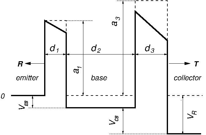
Figure 5: Schematics of typical transistor, where notations correspond to Equations (77) and (78) for $N=3$ and $\varepsilon=1$ with replacement: $b_{1}\to-\,V_{EB}$ (emitter-to-base voltage) and $b_{3}\to-\,V_{CB}$ (collector-to-base voltage). Potential values at layer edges are $V_{1,0}=a_{1}$, $V_{1,1}=a_{1}-V_{EB}$ ($a_{1}>0$), $V_{2,1}=V_{2,2}=-\,V_{EB}$ and $V_{3,2}=a_{3}-V_{EB}$, $V_{3,3}=a_{3}+V_{R}$ ($a_{3}>0$). Polarity is shown to be positive (left-to-right electron flow, $V_{EB}\,,V_{CB}>0$).

Similarly to the double-layer structure [see the general formula (29)], the transmission matrix for the total system is the product $\Lambda=\Lambda_{3}\Lambda_{2}\Lambda_{1}$, where the matrices $\Lambda_{1}$ and $\Lambda_{3}$ correspond to the barriers and the $\Lambda_{2}$-matrix to the space between the barriers. Setting $b_{1}\equiv-\,V_{EB}$, $b_{2}=0$ and $b_{3}\equiv-\,V_{CB}$, according to (77), we replace: $a\to a_{1}$ for $\Lambda_{1}$, $a\to-\,V_{EB}$ ($a_{2}=0$) for $\Lambda_{2}$ and $a\to a_{3}-V_{EB}$ for $\Lambda_{3}$. In the case of positive polarity, as shown in the figure, both the voltages are non-negative parameters. Applying next the replacement rules (79) in the terms (72), (73) and (76), we write the following explicit expressions for the matrices $\Lambda_{1}$ and $\Lambda_{3}$:

$$\kappa_{1} = \sqrt{-\,a_{1}}\,,~{}~{}\kappa_{2}=\sqrt{V_{EB}}\,,~{}~{}\kappa_{3}=\sqrt{V_{EB}-a_{3}}\,,$$

$$\alpha_{1} = (a_{1}-V_{EB}/2)d_{1}\,,~{}~{}\alpha_{3}=(a_{3}-V_{EB}-V_{CB}/2)d_{3}\,,$$

$$c_{1,1} = (a_{1}^{2}/2)(a_{1}-V_{EB})(d_{1}/V_{EB})^{2},$$

$$c_{1,2} = (a_{1}/2)(a_{1}-V_{EB})^{2}(d_{1}/V_{EB})^{2},$$

$$c_{3,1} = [(a_{3}-V_{EB})^{2}/2](a_{3}-V_{EB}-V_{CB})(d_{3}/V_{CB})^{2},$$

$$c_{3,2} = [(a_{3}-V_{EB})/2](a_{3}-V_{EB}-V_{CB})^{2}(d_{3}/V_{CB})^{2},$$

$$g_{1} = -\,\kappa_{1}^{-3}(V_{EB}/4d_{1}),~{}~{}g_{3}=-\,\kappa_{3}^{-3}(V_{CB}/4d_{3}).$$ (91)

The $\Lambda_{2}$-matrix is defined by (52) for $i=2$, where $k_{2}=\kappa_{2}\varepsilon^{-1}$ and $l_{2}=\varepsilon d_{2}$.

Below we examine the following two zero-thickness limits: (i) $\mu_{1}=\mu_{3}=\nu_{1}=\nu_{3}=1$ (points $P_{1,1}$) and (ii) $\mu_{1}=\mu_{3}=2$, $\nu_{1}=\nu_{3}=1$ (points $P_{2,1}$).

(i) $\delta$-potential model: The matrix multiplication yields the asymptotic representation in the limit as $\varepsilon\to 0$:

$$\lambda_{11} \to \cos(\kappa_{2}d_{2})-\kappa_{2}d_{3}\sin(\kappa_{2}d_{2}),$$

$$\lambda_{12} \to 0,$$

$$\lambda_{21} \to (\alpha_{1}+\alpha_{3})\cos(\kappa_{2}d_{2})+(c_{1,1}+c_{3,2})\kappa_{2}\sin(\kappa_{2}d_{2})-\varepsilon^{-1}\kappa_{2}\sin(\kappa_{2}d_{2}),$$

$$\lambda_{22} \to \cos(\kappa_{2}d_{2})-\kappa_{2}d_{1}\sin(\kappa_{2}d_{2}).$$ (92)

Here, the element $\lambda_{21}$ diverges as $\varepsilon\to 0$ and it will be finite if $\sin(\kappa_{2}d_{2})=0$, resulting in the resonance set

$$V_{EB,n}=(n\pi/d_{2})^{2},~{}~{}n=\overline{1,n_{0}}\,,$$ (93)

where the integer $n_{0}$ depends on the interval of admissible values of the bias potential $V_{EB}$. This interval is determined by the requirement that the barrier potential values $V_{1,1}$ and $V_{3,3}$ must be positive, leading to the inequalities $0<V_{EB}<a_{1}$ and $0<V_{EB}+V_{CB}<a_{3}$. Therefore the potential $V_{EB}$ is allowed to tune within the interval $0<V_{EB}<\min\{a_{1},\,a_{3}-V_{CB}\}$.

Thus, the limit transmission matrix is of the form (90) with

$$\alpha_{n}=\alpha_{1,n}+\alpha_{3,n}=(a_{1}-V_{EB,n}/2)d_{1}+(a_{3}-V_{EB,n}-V_{CB}/2)d_{3}>0.$$ (94)

realizing the $\delta$-potential defined on the resonance set described by Equation (93).

According to the general expressions (42) and (39), the transmission amplitude, being non-zero on this resonance set, is given by the formula (87), where $\theta_{n}=1$ and $k_{R,n}=\sqrt{k^{2}+V_{EB,n}+V_{CB}}\,$.

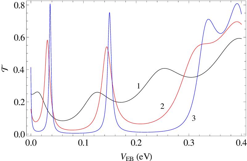
Figure 6: Transmission amplitude ${\cal T}$ as a function of emitter-to-base voltage $V_{EB}$ for parameter values: $E=0.1$ eV, $a_{1}=a_{3}=0.5$ eV, $a_{2}=0$, $V_{CB}=0.2$ eV, $d_{1}=d_{3}=2$ nm, $d_{2}=10$ nm. Computations have been carried out with powers $\mu_{1}=\nu_{1}=\mu_{3}=\nu_{3}=1$ (points $P_{1,1}$) and $\mu_{2}=2$, $\nu_{2}=0$. Squeezing scenario is displayed for $\varepsilon=0.5$ (curve 1, black), $0.25$ (curve 2, red) and $0.1$ (curve 3, blue). Location of all three peaks approaches set $\{V_{EB,n}\}$ given by Equation (93) with $n=1,\,2,\,3$.

The transmission amplitude ${\cal T}$ displayed in Figure 6 illustrates the convergence of the location of the peaks to the roots of Equation (93).

(ii) $\delta^{\prime}$-potential model: The three-lateral device can also be approximated by a $\delta^{\prime}$-interaction with a bias if we choose for the zero-thickness limit the powers $\mu_{1}=\mu_{2}=\mu_{3}=2$ and $\nu_{1}=\nu_{3}=1$. The multiplication of the matrices yields

$$\lambda_{11} \to \cos(\kappa_{1}d_{1})\cos(\kappa_{2}d_{2})\cos(\kappa_{3}d_{3})-(\kappa_{1}/\kappa_{2})\sin(\kappa_{1}d_{1})\sin(\kappa_{2}d_{2})\cos(\kappa_{3}d_{3})$$

$$-\,(\kappa_{1}/\kappa_{3})\sin(\kappa_{1}d_{1})\cos(\kappa_{2}d_{2})\sin(\kappa_{3}d_{3})$$

$$-(\kappa_{2}/\kappa_{3})\cos(\kappa_{1}d_{1})\sin(\kappa_{2}d_{2})\sin(\kappa_{3}d_{3}),$$

$$\lambda_{12} \to 0,$$

$$\lambda_{21} \to \kappa_{2}[g_{1}\sin(\kappa_{1}d_{1})\cos(\kappa_{3}d_{3})-g_{3}\cos(\kappa_{1}d_{1})\sin(\kappa_{3}d_{3})]\sin(\kappa_{2}d_{2})$$

$$+\,(\kappa_{3}g_{1}-\kappa_{1}g_{3})\sin(\kappa_{1}d_{1})\cos(\kappa_{2}d_{2})\sin(\kappa_{3}d_{3})$$

$$-\,\varepsilon^{-1}[\kappa_{1}\sin(\kappa_{1}d_{1})\cos(\kappa_{2}d_{2})\cos(\kappa_{3}d_{3})$$

$$+\,\kappa_{2}\cos(\kappa_{1}d_{1})\sin(\kappa_{2}d_{2})\cos(\kappa_{3}d_{3})+\kappa_{3}\cos(\kappa_{1}d_{1})\cos(\kappa_{2}d_{2})\sin(\kappa_{3}d_{3})$$

$$-\,(\kappa_{1}\kappa_{3}/\kappa_{2})\sin(\kappa_{1}d_{1})\sin(\kappa_{2}d_{2})\sin(\kappa_{3}d_{3})],$$

$$\lambda_{22} \to \cos(\kappa_{1}d_{1})\cos(\kappa_{2}d_{2})\cos(\kappa_{3}d_{3})-(\kappa_{2}/\kappa_{1})\sin(\kappa_{1}d_{1})\sin(\kappa_{2}d_{2})\cos(\kappa_{3}d_{3})$$ (95)

$$-\,(\kappa_{3}/\kappa_{1})\sin(\kappa_{1}d_{1})\cos(\kappa_{2}d_{2})\sin(\kappa_{3}d_{3})$$

$$-\,(\kappa_{3}/\kappa_{2})\cos(\kappa_{1}d_{1})\sin(\kappa_{2}d_{2})\sin(\kappa_{3}d_{3}),$$

where the notations for $\kappa_{1}\,,\kappa_{2}\,,\kappa_{3}$ and $g_{1}\,,g_{3}$ can be found in Equations (91). The arguments of the trigonometric functions are finite and the element $\lambda_{21}$ diverges as $\varepsilon\to 0$ because of the presence of the factor $\varepsilon^{-1}$. Therefore the only opportunity to define properly a point interaction is a full cancellation of all the terms at this factor, so that $\lambda_{21}$ becomes finite. As a result, this cancellation yields the following equation:

$${\kappa_{1}\kappa_{3}\over\kappa_{2}}\prod_{i=1}^{3}\tan(\kappa_{i}d_{i})=\sum_{i=1}^{3}\kappa_{i}\tan(\kappa_{i}d_{i}).$$ (96)

Using the resonance equation (96), we derive that the pair $\{\lambda_{11},\lambda_{22}\}$ admits the following sixteen representations:

$$\{\lambda_{11},\lambda_{22}\}=\{I_{1},I_{2},J_{1}^{-1},J_{2}^{-1}\}\times\{I_{1}^{-1},I_{2}^{-1},J_{1},J_{2}\},$$ (97)

where

$$I_{1} = {\cos(\kappa_{1}d_{1})\cos(\kappa_{2}d_{2})-(\kappa_{1}/\kappa_{2})\sin(\kappa_{1}d_{1})\sin(\kappa_{2}d_{2})\over\cos(\kappa_{3}d_{3})}\,,$$

$$I_{2} = -\,{\kappa_{1}\sin(\kappa_{1}d_{1})\cos(\kappa_{2}d_{2})+\kappa_{2}\cos(\kappa_{1}d_{1})\sin(\kappa_{2}d_{2})\over\kappa_{3}\sin(\kappa_{3}d_{3})}\,,$$

$$J_{1} = {\cos(\kappa_{2}d_{2})\cos(\kappa_{3}d_{3})-(\kappa_{3}/\kappa_{2})\sin(\kappa_{2}d_{2})\sin(\kappa_{3}d_{3})\over\cos(\kappa_{1}d_{1})}\,,$$

$$J_{2} = -\,{\kappa_{2}\sin(\kappa_{2}d_{2})\cos(\kappa_{3}d_{3})+\kappa_{3}\cos(\kappa_{2}d_{2})\sin(\kappa_{3}d_{3})\over\kappa_{1}\sin(\kappa_{1}d_{1})}\,.$$ (98)

These representations follow from the equations $I_{1}=I_{2}$, $J_{1}=J_{2}$ and $I_{1}J_{1}=1$, which can be checked using the condition (96). As a result, we have $\det\Lambda=\lambda_{11}\lambda_{22}=1$ if Equation (96) is fulfilled.

Equation (96) can be rewritten in the explicit form as follows

$$\sqrt{a_{1}/V_{EB}}\,\tanh(\sqrt{a_{1}}\,d_{1})+\sqrt{a_{3}/V_{EB}-1}\,\tanh(\sqrt{a_{3}-V_{EB}}\,d_{3})$$

$$=\left[1-\sqrt{a_{1}/V_{EB}}\,\sqrt{{a_{3}/V_{EB}}-1}\,\tanh(\sqrt{a_{1}}\,d_{1})\tanh(\sqrt{a_{3}-V_{EB}}\,d_{3})\right]$$

$$\times\tan(\sqrt{V_{EB}}\,d_{2}).$$ (99)

This form shows the existence of the roots forming a resonance set $\Sigma=\{V_{EB,n}\}$. Inserting next these roots into Equations (98), one can get the discrete values of the diagonal elements $\lambda_{11,n}$ and $\lambda_{22,n}$ of the matrix set $\Lambda|_{\Sigma}$. One can write then $\theta_{n}:=\lambda_{11,n}=\lambda_{22,n}^{-1}=I_{1,n}=I_{2,n}=J_{1,n}^{-1}=J_{2,n}^{-1}$. Finally, one can represent the off-diagonal element $\lambda_{21,n}=\alpha_{n}$ as

$$\alpha_{n} = a_{1}^{-3/2}(V_{EB,n}/4d_{1})\sinh(\sqrt{a_{1}}\,d_{1})$$ (100)

$$\times [\sqrt{V_{EB,n}}\cosh(\sqrt{a_{3}-V_{EB,n}}\,d_{3})\sin(\sqrt{V_{EB,n}}\,d_{2})$$

$$- \sqrt{a_{3}-V_{EB,n}}\sinh(\sqrt{a_{3}-V_{EB,n}}\,d_{3})\cos(\sqrt{V_{EB,n}}\,d_{2})]$$

$$- (a_{3}-V_{EB,n})^{-3/2}(V_{CB}/4d_{3})\sinh(\sqrt{a_{3}-V_{EB,n}}\,d_{3})$$

$$\times [\sqrt{V_{EB,n}}\cosh(\sqrt{a_{1}}\,d_{1})\sin(\sqrt{V_{EB,n}}\,d_{2})$$

$$- \sqrt{a_{1}}\sinh(\sqrt{a_{1}}\,d_{1})\cos(\sqrt{V_{EB,n}}\,d_{2})].$$

Similarly to the double-layer structure with the limit transmission matrix (85), we refer this one-point interaction to as the $\delta^{\prime}$-potential because $\lambda_{11,n}\,,\,\lambda_{22,n}\neq 1$. The transmission amplitude is given by the same formula (87) in which $\theta_{n}=\lambda_{11,n}$ and $\alpha_{n}=\lambda_{21,n}$ is given by the expression (100).

7 Concluding remarks

In the present work we addressed the family of point interactions as the zero-thickness limit of heterostructures composed of several layers. The latter have energy diagrams stemming from tilted linear potentials that arise as a result of the application of external electric fields. The analysis starts from the solution of the one-dimensional stationary Schrödinger equation for the structure with finite size using the transfer matrix approach. Within this approach, we find the transmission matrices for each layer; their product quantifies the penetration amplitude of electrons through the whole system. In order to realize point interactions we introduce a squeezing parameter $\varepsilon>0$ in the structural parameters of the system (layer width, potentials at layer edges, etc.) leading to shrinking the thickness of the system as $\varepsilon\to 0$. In this limit the potential values at the interfaces of layers must go to infinity if we wish to create a point interaction in the squeezed limit. At $\varepsilon=1$, the structural parameters correspond to realistic values of the device.

One of interesting features discovered in the previous publications [17, 42, 43, 44, 47, 48, 50] is the appearance of electron tunneling through one-point barriers that occurs at some discrete values of system parameters, whereas beyond these values the system behaves as a fully reflecting wall. The origin of this phenomenon is an oscillating behavior of particle transmission. Surprisingly, as the system shrinks to a point, the oscillating regular function that describes the transmission amplitude, converges pointwise to the function with non-zero finite values only at some discrete points in the space of system parameters, whereas beyond this (resonance) set, the system acts a fully reflecting wall (see, e.g., Figure 1 in [17]). In other words, the maxima of the oscillating amplitude correspond in the squeezing limit to the set of extremely sharp peaks. On the other hand, in many devices the oscillating behavior of transmitted particles appears as a function of tuning some controllable (not system) parameters. For instance, in the typical point transistor, an emitter-to-base voltage may be served as such a parameter. Indeed, the electron flow across this device is an oscillating function of this voltage. In this regard, it is of interest to construct the point interactions with a resonance set controllable by parameters applied externally and this is the main goal of the present paper.

In conclusion, in the present paper we have tried to develop the general approach on how to realize the point interactions as a zero-thickness limit of structures composed of an arbitrary number of layers with biased potentials. This approach is specified by the examples describing one layer, the double- and three-layer systems. The piecewise linear potentials are not required to have any distributional limit as $\varepsilon\to 0$. Despite this, the $\varepsilon\to 0$ limit of the transmission matrices has been shown to exist enable us to compute analytically the transmission amplitude. The most interesting phenomenon discussed in the present paper is the appearance of the resonant transmission through a $\delta$-like barrier in the presence of an adjacent well. The origin of this effect emerges from the fact that the particle transmission across a well has an oscillating behavior. This behavior keeps to be of the same nature after tunneling through a barrier. Therefore in the squeezed limit this oscillating transforms into the function with non-zero values only at discrete points, whereas on the intervals between these points, this function converges pointwise to zero resulting in blocking the tunneling trough the barrier.

Acknowledgments

One of us (A.V.Z) acknowledges partial financial support from the National Academy of Sciences of Ukraine (project No. 0117U000238). G.P.T. acknowledges support by the European Commission under project NHQWAVE (MSCA-RISE 691209). Y.Z. acknowledges support from the Department of Physics and Astronomy of the National Academy of Sciences of Ukraine under project No. 0117U000240.

References

References

- [1] Y.N. Demkov, V.N. Ostrovskii, Zero-Range Potentials and Their Applications in Atomic Physics, Plenum Press, New York, 1988 (Leningrad University Press, Leningrad, 1975).
- [2] Albeverio S, Gesztesy F, Høegh-Krohn R, H. Holden H. Solvable Models in Quantum Mechanics, second ed. with appendix by P. Exner, AMS Chelsea, Providence, RI, 2005.
- [3] Albeverio S, Kurasov P. Singular Perturbations of Differential Operators: Solvable Schrödinger-Type Operators, Cambridge University Press, Cambridge, 1999.
- [4] Šeba P. Some remarks on the -interaction in one dimension. Rep Math Phys. (1986) 24:111-20.
- [5] Kurasov P. Distribution theory for discontinuous test functions and differential operators with generalized coefficients. J Math Anal Appl. (1996) 201:297-323. doi: 10.1006/jmaa.1996.0256
- [6] Coutinho FAB, Nogami Y, Perez JF. Generalized point interactions in one-dimensional quantum mechanics. J Phys A Math Gen. (1997) 30:3937-45. doi: 10.1088/0305-4470/30/11/021
- [7] Albeverio S, Da̧browski L, Kurasov P. Symmetries of Schrödinger operators with point interactions. Lett Math Phys. (1998) 45:33-47. doi: 10.1023/A:1007493325970
- [8] Coutinho FAB, Nogami Y, Tomio L. Many-body system with a four-parameter family of point interactions in one dimension. J Phys A Math Gen. (1999) 32:4931-42. doi: 10.1088/0305-4470/32/26/311
- [9] Albeverio S, Nizhnik L. On the number of negative eigenvalues of a one-dimensional Schrödinger operator with point interactions. Lett Math Phys (2003) 65:27-35. doi: 10.1023/A:1027396004785
- [10] Nizhnik LP. A Schrödinger operator with -interaction. Funct Anal Appl. (2003) 37:72-4. doi: 10.1023/A:1022932229094
- [11] Nizhnik LP. A one-dimensional Schrödinger operator with point interactions on Sobolev spaces. Funct Anal Appl. (2006) 40:143-7. doi: 10.1007/s10688-006-0022-3
- [12] Albeverio S, Cacciapuoti C, Finco D. Coupling in the singular limit of thin quantum waveguides. J Math Phys. (2007) 48:032103. doi: 10.1063/1.2710197
- [13] Cacciapuoti C, Exner P. Nontrivial edge coupling from a Dirichlet network squeezing: the case of a bent waveguide. J Phys A Math Theor. (2007) 40:F511-23. doi: 10.1088/1751-8113/40/26/F02
- [14] Turek O, Cheon T. Threshold resonance and controlled filtering in quantum star graphs. Europhys Lett. (2012) 98:50005. doi: 10.1209/0295-5075/98/50005
- [15] Turek O, Cheon T. Potential-controlled filtering in quantum star graphs. Ann Phys (NY) (2013) 330:104-41. doi: 10.1016/j.aop.2012.11.011
- [16] Zolotaryuk AV, Zolotaryuk Y. Controllable resonant tunnelling through single-point potentials: A point triode. Phys Lett A (2015) 379:511-7. doi: 10.1016/j.physleta.2014.12.016
- [17] Zolotaryuk AV, Zolotaryuk Y. A zero-thickness limit of multilayer structures: a resonant-tunnelling -potential. J Phys A Math Theor. (2015) 48:035302. doi: 10.1088/1751-8113/48/3/035302
- [18] Asorey M, Ibort A, Marmo G. Global theory of quantum boundary conditions and topology change. Int J Mod Phys A (2005) 20:1001-26. doi: 10.1142/S0217751X05019798
- [19] Cheon T, Fülöp T, Tsutsui I. Symmetry, duality, and anholonomy of point interactions in one dimension. Ann Phys (NY) (2001) 294:1-23. doi: 10.1006/aphy.2001.6193
- [20] Tsutsui I, Fülöp T, Cheon T. Möbius structure of the special space of Schrödinger operators with point interaction. J Math Phys. (2001) 42:5687-97. doi: 10.1063/1.1415432
- [21] Cheon T, Shigehara T. Realizing discontinuous wave functions with renormalized short-range potentials. Phys Lett A (1998) 243:111-6.
- [22] Exner P, Neidhardt H, Zagrebnov VA. Potential Approximations to : An inverse Klauder phenomenon with norm-resolvent convergence. Commun Math Phys. (2001) 224:593-612. doi: 10.1007/s002200100567
- [23] Albeverio S, Nizhnik L. Approximation of general zero-range potentials. Ukr Mat Zh. (2000) 52:582-9; Albeverio S, Nizhnik L. Ukr Math J. (2000) 52:664-72. doi: 10.1007/BF02487279
- [24] Albeverio S, Nizhnik L. A Schrödinger operator with a -interaction on a Cantor set and Krein-Feller operators. Mathematische Nachrichten (2006) 279:467-76. doi: 10.1002/mana.200310371
- [25] Albeverio S. Nizhnik L. Schrödinger operators with nonlocal point interactions. J Math Anal Appl. (2007) 332:884-95. doi: 10.1016/j.jmaa.2006.10.070
- [26] Albeverio S, Nizhnik L. Schrödinger operators with nonlocal potentials. Methods Funct Anal Topology (2013) 19:199-210. Available online at: http://mfat.imath.kiev.ua/article/?id=698
- [27] Fassari S, Rinaldi F. On the spectrum of the Schrödinger Hamiltonian with a particular configuration of three one-dimensional point interactions. Rep Math Phys. (2009) 64:367-93. doi: 10.1016/S0034-4877(10)00004-2
- [28] Albeverio S, Fassari S, Rinaldi F. A remarkable spectral feature of the Schrödinger Hamiltonian of the harmonic oscillator perturbed by an attractive -interaction centred at the origin: double degeneracy and level crossing. J Phys A Math Theor. (2013) 46:385305. doi: 10.1088/1751-8113/46/38/385305
- [29] Albeverio S, Fassari S, Rinaldi F. The Hamiltonian of the harmonic oscillator with an attractive -interaction centred at the origin as approximated by the one with a triple of attractive -interactions. J Phys A Math Theor. (2016) 49:025302. doi: 10.1088/1751-8113/49/2/025302
- [30] Golovaty Y. Two-parametric -interactions: approximation by Schrödinger operators with localized rank-two perturbations. J Phys A Math Theor. (2018) 51:255202. doi: 10.1088/1751-8121/aac110
- [31] Brasche JF, Nizhnik LP. One-dimensional Schrödinger operators with general point interactions. Methods Funct Anal Topology (2013) 19:4-15. Available online at: http://mfat.imath.kiev.ua/article/?id=675
- [32] Gadella M, Negro J, Nieto LM. Bound states and scattering coefficients of the potential. Phys Lett A (2009) 373:1310-3. doi: 10.1016/j.physleta.2009.02.025
- [33] Gadella M, Glasser ML, Nieto LM. One dimensional models with a singular potential of the type . Int J Theor Phys. (2011) 50 2144-52. doi: 10.1007/s10773-010-0641-6
- [34] Lange RJ. Potential theory, path integrals and the Laplacian of the indicator. J High Energy Phys. (2012) JHEP11:1-32. doi: 10.1007/JHEP11(2012)032
- [35] Lange RJ. Distribution theory for Schrödinger’s integral equation. J Math Phys. (2015) 56:122105. doi.org/10.1063/1.4936302
- [36] Gadella M, García-Ferrero MA, González-Martín S, Maldonado-Villamizar FH. The infinite square well with a point interaction: A discussion on the different parameterizations. Int J Theor Phys. (2014) 53:1614-27. doi: 10.1007/s10773-013-1959-7
- [37] Kulinskii VL, Panchenko DY. Physical structure of point-like interactions for one-dimensional Schrödinger operator and the gauge symmetry. Physica B (2015) 472:78-83. doi: 10.1016/j.physb.2015.05.011
- [38] Gadella M, Mateos-Guilarte J, Muñoz-Castañeda JM, Nieto LM. Two-point one-dimensional - interactions: non-abelian addition law and decoupling limit. J Phys A Math Theor. (2016) 49:015204. doi: 10.1088/1751-8113/49/1/015204
- [39] Fassari S, Gadella M, Glasser ML, Nieto LM. Spectroscopy of a one-dimensional V-shaped quantum well with a point impurity. Ann Phys (NY) (2018) 389:48-62. doi: 10.1016/j.aop.2017.12.006
- [40] Fassari S, Gadella M, Glasser ML, Nieto LM. Level crossings of eigenvalues of the Schrödinger Hamiltonian of the isotropic harmonic oscillator perturbed by a central point interaction in different dimensions. Nanosyst Phys Chem Math. (2018) 9:179-86. doi: 10.17586/2220-8054-2018-9-2-179-186
- [41] Fassari S, Gadella M, Glasser ML, Nieto LM, Rinaldi F. Spectral properties of the two-dimensional Schrödinger Hamiltonian with various solvable confinements in the presence of a central point perturbation. Phys Scr. (2019) 94:055202. doi: 10.1088/1402-4896/ab0589
- [42] Christiansen PL, Arnbak NC, Zolotaryuk AV, Ermakov VN, Gaididei YB. On the existence of resonances in the transmission probability for interactions arising from derivatives of Dirac’s delta function. J Phys A Math Gen. (2003) 36:7589-600. doi: 10.1088/0305-4470/36/27/311
- [43] Zolotaryuk AV, Christiansen PL, Iermakova SV. Scattering properties of point dipole interactions. J Phys A Math Gen. (2006) 39:9329-38. doi: 10.1088/0305-4470/39/29/023
- [44] Toyama FM, Nogami Y. Transmission-reflection problem with a potential of the form of the derivative of the delta function. J Phys A Math Theor. (2007) 40:F685-90. doi: 10.1088/1751-8113/40/29/F05
- [45] Zolotaryuk AV. Boundary conditions for the states with resonant tunnelling across the -potential. Phys Lett A (2010) 374:1636-41. doi: 10.1016/j.physleta.2010.02.005
- [46] Zolotaryuk AV, Zolotaryuk Y. Intrinsic resonant tunneling properties of the one-dimensional Schrödinger operator with a delta derivative potential. Int J Mod Phys B (2014) 28:1350203. doi: 10.1142/S0217979213502032
- [47] Golovaty YD, Man’ko SS. Solvable models for the Schrödinger operators with -like potentials. Ukr Math Bull. (2009) 6:169-203. Available online at: https://arxiv.org/abs/0909.1034
- [48] Golovaty YD, Hryniv RO, On norm resolvent convergence of Schrödinger operators with -like potentials. J Phys A Math Theor. (2010) 43:155204. doi: 10.1088/1751-8113/43/15/155204
- [49] Golovaty Y. Schrödinger operators with -like potentials: Norm resolvent convergence and solvable models. Methods Funct Anal Topology (2012) 18:243-55. Available online at: http://mfat.imath.kiev.ua/article/?id=633
- [50] Golovaty YD, Hryniv RO. Norm resolvent convergence of singularly scaled Schrödinger operators and -potentials. Proc R Soc Edinb. (2013) 143A:791-816. doi: 10.1017/S0308210512000194
- [51] Golovaty Y. 1D Schrödinger operators with short range interactions: two-scale regularization of distributional potentials. Integr Equ Oper Theory (2013) 75:341-62. doi: 10.1007/s00020-012-2027-z
- [52] Zolotaryuk AV. Families of one-point interactions resulting from the squeezing limit of the sum of two- and three-delta-like potentials. J Phys A Math Theor. (2017) 50:225303. doi: 10.1088/1751-8121/aa6dc2
- [53] Zolotaryuk AV. A phenomenon of splitting resonant-tunneling one-point interactions. Ann Phys (NY) (2018) 396:479–94. doi: 10.1016/j.aop.2018.07.030
- [54] Calçada M, Lunardi JT, Manzoni LA. Salecker-Wigner-Peres clock and double-barrier tunneling. Phys Rev A (2009) 79:012110. doi: 10.1103/PhysRevA.79.012110
- [55] Lunardi JT, Manzoni LA, Monteiro W. Remarks on point interactions in quantum mechanics. J Phys Conf Series (2013) 410:012072. doi: 10.1088/1742-6596/410/1/012072
- [56] Calçada M, Lunardi JT, Manzoni LA, Monteiro W. Distributional approach to point interactions in one-dimensional quantum mechanics. Front Phys. (2014) 2:23. doi: 10.3389/fphy.2014.00023
- [57] Lee MA, Lunardi JT, Manzoni LA, Nyquist EA. On the generalized Hartman effect for symmetric double-barrier point potentials. J Phys Conf Series (2015) 574:012066. doi: 10.1088/1742-6596/574/1/012066
- [58] Lee MA, Lunardi JT, Manzoni LA, Nyquist EA. Double general point interactions: symmetry and tunneling times. Front Phys. (2016) 4:10. doi: 10.3389/fphy.2016.00010
- [59] Asorey M, Garciá-Alvarez D, Muñoz-Castañeda JM. Casimir effect and global theory of boundary conditions. J Phys A Math Theor. (2006) 39:6127-36. doi: 10.1088/0305-4470/39/21/S03
- [60] Asorey M, Muñoz-Castañeda JM. Vacuum boundary effects. J Phys A Math Theor. (2008) 41:304004. doi: 10.1088/1751-8113/41/30/304004
- [61] Guilarte JM, Muñoz-Castañeda JM. Double-delta potentials: one dimensional scattering. The Casimir effect and kink fluctuations. Int J Theor Phys. (2011) 50:2227-41. doi: 10.1007/s10773-011-0723-0
- [62] Asorey M, Muñoz-Castañeda JM. Attractive and repulsive Casimir vacuum energy with general boundary conditions. Nucl Phys B (2013) 874:852-76. doi: 10.1016/j.nuclphysb.2013.06.014
- [63] Muñoz-Castañeda JM, Guilarte JM, Mosquera AM. Quantum vacuum energies and Casimir forces between partially transparent -function plates. Phys Rev D (2013) 87:105020. doi: 10.1103/PhysRevD.87.105020
- [64] Muñoz-Castañeda JM, Kirsten K, Bordag M. QFT over the finite line. Heat kernel coefficients, spectral zeta functions and selfadjoint extensions. Lett Math Phys. (2015) 105:523549. doi: 10.1007/s11005-015-0750-5
- [65] Muñoz-Castañeda JM, Guilarte JM. - generalized Robin boundary conditions and quantum vacuum fluctuations. Phys Rev D (2015) 91:025028. doi: 10.1103/PhysRevD.91.025028
- [66] Bordag M, Muñoz-Castañeda JM. Quantum vacuum interaction between two sine-Gordon kinks. J Phys A Math Theor. (2012) 45:374012. doi: 10.1088/1751-8113/45/37/374012
- [67] Hennig D, Tsironis GP. Wave transmission in nonlinear lattices. Phys. Rep. (1999) 307:333-432. doi: 10.1016/S0370-1573(98)00025-8
- [68] Nieto LM, Gadella M, Guilarte JM, Muñoz-Castañeda JM, Romaniega C. Towards modelling QFT in real metamaterials: Singular potentials and self-adjoint extensions. J Phys Conf Series (2017) 839:012007. doi: 10.1088/1742-6596/839/1/012007
- [69] Konno K, Nagasawa T, Takahashi R. Effects of two successive parity-invariant point interactions on one-dimensional quantum transmission: Resonance conditions for the parameter space. Ann Phys (NY) (2016) 375:91-104. doi: 10.1016/j.aop.2016.09.012
- [70] Konno K, Nagasawa T, Takahashi R. Resonant transmission in one-dimensional quantum mechanics with two independent point interactions: Full parameter analysis. Ann Phys (NY) (2017) 385:729-43. doi: 10.1016/j.aop.2017.08.031
- [71] Tsu R, Esaki L. Tunneling in a finite superlattice. Appl Phys Lett. (1973) 22:562-4.
- [72] Chang LL, Esaki L, Tsu R. Resonant tunneling in semiconductor double barriers. Appl Phys Lett. (1974) 24:593-5.
- [73] Esaki L, Chang LL. New transport phenomenon in a semiconductor “superlattice”. Phys Rev Lett. (1974) 33:495-8.
- [74] Lui WW, Fukuma M. Exact solution of the Schrödinger equation across an arbitrary one-dimensional piecewise-linear potential barrier. J Appl Phys. (1986) 60:1555-9. doi: 10.1063/1.337788
- [75] Jogai B, Wang KL. Dependence of tunneling current on structural variations of superlattice devices. Appl Phys Lett. (1985) 46:167-8. doi: 10.1063/1.95671