Making targeted black-box evasion attacks effective and efficient

Abstract.

We investigate how an adversary can optimally use its query budget for targeted evasion attacks against deep neural networks in a black-box setting. We formalize the problem setting and systematically evaluate what benefits the adversary can gain by using substitute models. We show that there is an exploration-exploitation tradeoff in that query efficiency comes at the cost of effectiveness. We present two new attack strategies for using substitute models and show that they are as effective as previous “query-only” techniques but require significantly fewer queries, by up to three orders of magnitude. We also show that an agile adversary capable of switching through different attack techniques can achieve pareto-optimal efficiency. We demonstrate our attack against Google Cloud Vision showing that the difficulty of black-box attacks against real-world prediction APIs is significantly easier than previously thought (requiring $\approx$500 queries instead of $\approx$20,000 as in previous works).

1. Introduction

The immense surge in the popularity of machine learning applications in recent years has been accompanied by concerns about their security and privacy. One such concern is evasion. Given a machine learning classifier (victim) and a particular input (goal), evasion is the process of finding an adversarial example (Biggio et al., 2013; Szegedy et al., 2013) that is sufficiently close to the goal, but will fool the victim classifier into outputting a different class label than that for the goal. When the adversary aims for a specific misclassified label, evasion is said to be targeted. For image classifiers, the difference between the adversarial example and goal images is imperceptible to humans.

Early techniques for finding adversarial examples against deep neural networks (DNNs) for image classification assumed a white-box setting, where the adversary knows the architecture and weights of the victim DNN (Szegedy et al., 2013; Goodfellow et al., 2015a). Since DNN cost functions are differentiable, these techniques calculated minimal changes (perturbations) to images which resulted in the DNN misclassifying the modified image. Later work addressed the black-box setting, where this perturbation cannot be directly calculated. Papernot et al (Papernot et al., 2016) demonstrated that adversarial examples exhibit transferability: adversarial examples for one DNN (substitute model) are likely to be adversarial to another DNN (victim model) when they are trained on datasets with a similar distribution. Liu et al (Liu et al., 2016) empirically demonstrated that using an ensemble of substitute models instead of a single one results in better transferability. We call the state-of-the-art techniques in this category, such as  (Liu et al., 2016) which rely exclusively on the use of ensembles as Ens. These are efficient in that the adversary needs to access the victim DNN only once (to test the adversarial example) but are not effective in targeted evasion because they may not always result in successful adversarial examples.

An alternative approach for targeted black-box evasion is where the adversary repeatedly queries the prediction API of a victim DNN, and estimates its gradient solely based on the responses to the queries. We call this class of techniques (Chen et al., 2017; Brendel et al., 2018; Ilyas et al., 2018b), query-only: QO. These techniques are highly effective, reaching up to 100%. But they are inefficient. For example, even state-of-the-art methods (Ilyas et al., 2018a) require up to 10 000 API queries for Google’s Inception v3 (Szegedy et al., 2016) to reach a success rate of 95.6% assuming that the API returns probability scores for all labels. Real-life DNN APIs often work in a partial information (PI) setting (Ilyas et al., 2018b), where the API only returns the top-k scores which further degrades the efficiency of QO techniques: the state-of-the-art to the best of our knowledge is (Ilyas et al., 2018b) which reports requiring 350,000 queries reach a success rate of 93.6% on this network in a PI setting.

Figure 1. Comparison of targeted black-box attacks against a partial information ResNet-152 model using different strategies: QO (Ilyas et al., 2018b) vs. EQ (using MIFGSM for gradient estimation (Dong et al., 2018), followed by QO), vs. a fully agile adversary EPP_RQ switching through all methods (Sec.4.6).

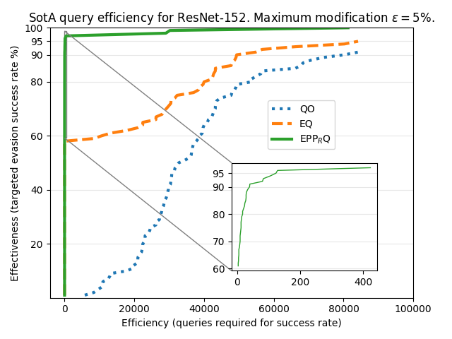
In this paper, we ask if we can design targeted black-box evasion techniques that are simultaneously efficient and effective. We argue that a realistic solution should (a) be designed for the partial-information setting since real-life APIs often use this setting; and (b) use ensembles because of the widespread availability of public, pre-trained models. Our contributions are as follows:

• We show that Ens followed by QO (EQ) can outperform pure QO techniques (Sec. 4.6).

• We present PRISM and PRISM_R, two new targeted black-box evasion techniques that (a) starts from an input with the target label, and (b) repeatedly query the victim API (within a query budget) while concurrently using an ensemble to estimate victim’s gradient in a PI setting. (Sec. 3.2). We show that the effectiveness of PRISM is comparable to QO on publicly available ImageNet models while typically requiring fewer victim queries by three orders of magnitude (Sec. 4.5).

• We systematically compare the different evasion approaches to show that an agile adversary can switch through these approaches in a particular order to achieve optimal efficiency, e.g. 13219 queries on average to reach the effectiveness 94% on Inception v3 in PI setting (Sec. 4.6).

• We demonstrate the real-world applicability of PRISM by producing a targeted adversarial example against Google Cloud Vision, reducing the number of queries required from an estimate of 20,000 queries (Ilyas et al., 2018b) to approximately 500 (Sec. 4.7).

Figure 1 shows the benefit of attacker agility by comparing different strategies: QO vs. EQ vs. a fully agile adversary EPP_RQ who switches through all methods (Ens, PRISM, PRISM_R and QO). In Section 5, we discuss possible reasons why the PRISM approach is effective.

2. Preliminaries

We first lay out definitions of frequently used concepts and functions in this work, with the focus on the image domain.

2.1. API definitions

Classifier,

clf: a function that maps an arbitrary input image $\mathbf{x}\in{\rm[0,1]}^{{\rm c}\times{\rm w}\times{\rm h}}$ to a vector of probabilities $\mathbf{p}\in[0,1]^{{\rm N}}$, denoting clf’s confidence in assigning $\mathbf{x}$ to any of the pre-defined classes $\{{\rm 1},\dots,{\rm N}\}$. The elements of $\mathbf{p}$ sum to 1. Here ${\rm c}$ refers to the number of color channels, ${\rm w}$ to the width and ${\rm h}$ to the height of input $\mathbf{x}$. A deep neural network dnn is a particular type of clf parameterized with $M$ sequential functions:

(1) $$\texttt{dnn}(\mathbf{x})=f_{M}\circ f_{M-1}\circ\dots f_{2}\circ f_{1}\circ\mathbf{x},$$

where each function $f_{i}(\mathbf{z})$ can be expressed as $\sigma_{i}(\mathbf{w}_{i}^{T}\mathbf{z}+\mathbf{b}_{i})$, where $\sigma_{i}$ is a (nonlinear) function, $\mathbf{w}_{i}$ is a weight matrix and $\mathbf{b}_{i}$ is a bias vector. In this work, we focus on dnn-based image classifiers. In a typical dnn, $\sigma_{i}$ is selected as a differentiable function. Therefore, it can calculate the gradient of classification error ($\nabla_{x}\texttt{dnn}$) in order to minimize this error easily in the training procedure (Goodfellow et al., 2016).

Preprocessor,

pre: A function that receives an input $\mathbf{x}\in{\rm I\!R}^{{\rm c}\times{\rm h}\times{\rm w}}$ and produces an output $\mathbf{x}^{\prime}\in{\rm I\!R}^{{\rm c^{\prime}}\times{\rm h^{\prime}}\times{\rm w^{\prime}}}$, and is primarily used for formatting, normalizing and resizing input $\mathbf{x}$ before it is classified by dnn, since dnn only processes fixed input sizes. pre can be used to break the differentiability property of dnn and act as a form of defense (shattered gradients, (Athalye et al., 2018)).

Postprocessor,

post: A function that receives input $\mathbf{p}\in{\rm I\!R}^{{\rm N}}$ and produces an output $\mathbf{p^{\prime}}\in{\rm I\!R}^{{\rm N^{\prime}}}$. It is used for formatting the output $\mathbf{p}$ of dnn, both for readability and limiting information from dnn. Common choices are:

• Identity function: $\texttt{post}_{I}(\mathbf{x})\leftarrow\texttt{I}(\mathbf{x})~{}\forall x$

• Label-only: $\texttt{post}_{\mathcal{L}}(\mathbf{x})\leftarrow\operatorname*{arg\,max}(\mathbf{x})$, i.e. the index $i\in\{1,...,N\}$ with the largest value in $x$.

• Top-k: $\texttt{post}_{\rm k}(\mathbf{x})\leftarrow\mathbf{w}_{\rm k}\cdot\mathbf{x}\in{\rm I\!R}^{{\rm N}}$, such that $\mathbf{w}_{\rm k,i}\leftarrow 1$ iff $i$ is among the ${\rm k}$ first values in sorted($\mathbf{x}$), where $\mathbf{x}$ is sorted in descending order. $\mathbf{w}_{\rm k,i}\leftarrow 0$ for others.

API:

A combination of pre, dnn and post that responds to arbitrary client, CLI, queries $\mathbf{x}$ with the following response:

(2) $${}_{\texttt{pre}}\texttt{API}_{\texttt{post}}(\mathbf{x})=\texttt{post}\circ\texttt{dnn}\circ\texttt{pre}\circ\mathbf{x}$$

An ideal API always responds to CLI’s queries $\mathbf{x}$, as long as $\mathbf{x}$ is not malformatted. Prior work in black-box adversarial examples however typically do not use preprocessing on APIs $\texttt{pre}(\mathbf{x})=\texttt{I}(\mathbf{x})=\mathbf{x}$. In this paper, we only focus on preprocessing that resizes input correctly for dnn.

White-box access:

CLI knows the precise definition of every intermediate function applied on any arbitrary input $\mathbf{x}$. Moreover, $\texttt{pre}(\mathbf{x})=\texttt{post}(\mathbf{x})=\texttt{I}(\mathbf{x})$, i.e. CLI has access to all of dnn’s outputs.

Gray-box access:

CLI does not know the full definition of pre and post or the network parameters of dnn, but may know other information such as the architecture, hyper-parameters, training method and the training set of dnn (Meng and Chen, 2017).

Black-box access:

CLI does not know the exact forms of any intermediate functions. Different authors define the minutiae of black-box API differently, we adapt these as follows (in order of decreasing privilege):

• Maximum information ($\texttt{API}_{I}$): dnn is secret, while CLI has access to probabilities or logits from dnn for arbitrary input $\mathbf{x}$  (Ilyas et al., 2018a).

• Partial information ($\texttt{API}_{k}$): CLI has access to top-k output from dnn for arbitrary input $\mathbf{x}$ (Ilyas et al., 2018b). Generally, a realistic API has a long probability list $\mathbf{p}\in{\rm I\!R}^{{\rm N}}$ with $N\geq 1000$ and returns a small subset of this list ($k\ll N$).

• Label-only ($\texttt{API}_{\mathcal{L}}$): CLI has access only to labels from dnn for arbitrary input $\mathbf{x}$ (Ilyas et al., 2018b).

2.2. Adversarial example definitions

Adversarial example:

The adversary aims to produce an adversarial example $x_{\rm adv}$ that is very similar to a goal image $x_{\rm goal}$, but evades classification by API: $\texttt{API}(x_{\rm adv})\neq\texttt{API}(x_{\rm goal})$ (non-targeted evasion). The similarity between $x_{\rm goal}$ and $x_{\rm adv}$ is often evaluated by an $L_{p}$-norm (Sharif et al., 2018): $\left\lVert x_{\rm goal}-x_{\rm adv}\right\rVert_{\rm p}$. In this work, we set $p=\infty$ as is common. In targeted evasion, adversarial examples require that $y^{\prime}\leftarrow\texttt{API}(x_{\rm adv})$ for a pre-defined class $y^{\prime}\neq\texttt{API}(x_{\rm goal})$. Targeted evasion is described in Equation 3.

(3) $$\begin{split}y^{\prime}&\leftarrow\texttt{API}(x_{\rm adv})\\ \text{s.t.~{}}&\left\lVert x_{\rm goal}-x_{\rm adv}\right\rVert_{\infty}\leq\epsilon\\ x_{\rm goal},x_{\rm adv}\in&~{}[0,1]^{\rm{c}\times w\times h},\end{split}$$

where $\epsilon$ is the allowed perturbation size.

White-box attacker, $\mathcal{A}_{\rm Wbox}$, is a malicious client that has white-box access to API which it tries to evade. Since $\mathcal{A}_{\rm Wbox}$ knows the precise definition of every intermediate function in dnn inside API, it is able to calculate the gradient of the classification error with respect to the input image: $\nabla_{x}\texttt{dnn}$. It uses this information to modify $x_{\rm adv}$. Existing evasion methods such as single-step fast gradient sign method FGSM (Goodfellow et al., 2015b) and iterative version of it I-FGSM (Kurakin et al., 2016) find adversarial example $x_{\rm adv}$ by maximizing the cross entropy loss function of dnn under $L_{\infty}$-norm.

Black-box attacker, $\mathcal{A}_{\rm Bbox}$, is a malicious client that has black-box access to $\texttt{API}^{\prime}$ that it tries to evade. Rotations and translation operations are often enough to create non-targeted evasion in black-box APIs (Engstrom et al., 2018). However, in order to create targeted adversarial examples with a small perturbation, an approximation to the gradient information, $\hat{\texttt{G}}_{\texttt{dnn}}^{\prime}$, of the target classifier $\texttt{dnn}^{\prime}$ becomes necessary. There are two predominant ways of obtaining this information: (a) gradient approximation through transferability and (b) finite-difference methods.

Transferability:

An adversarial example developed for evading one API (dnn) can be also adversarial to another $\texttt{API}^{\prime}$ ($\texttt{dnn}^{\prime}$), i.e.

(4) $$\begin{split}y^{\prime}&\leftarrow\ \texttt{API}^{\prime}(x_{\rm adv})\\ \text{s.t.~{}}&\text{Equation (\ref{eq:adv})}\end{split}$$

Recently, Adam et al. (Adam et al., 2019) found that the cosine similarity between the gradient $\nabla_{x}\texttt{dnn'}$ and the available gradient $\nabla_{x}\texttt{dnn}$ is a reliable estimator for transferability. Thus, implicitly the following approximation occurs during transferability:

(5) $$\nabla_{x}\texttt{dnn}\approx\nabla_{x}\texttt{dnn}^{\prime}$$

Liu et al. (Liu et al., 2016) states that transferability depends on the architectural similarity of $\texttt{dnn}^{\prime}$ and dnn.

Baseline transferability attack:

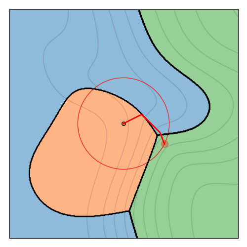
Adversary $\mathcal{A}_{Bbox}$ has a label-only black-box access to $\texttt{API}^{\prime}$. It tries to evade $\texttt{API}^{\prime}$ by creating adversarial examples using many available APIs and relies on the transferability property holds for the attacker’s adversarial examples. Current state-of-the-art transferability attacks use ensembles of pre-trained DNNs as dnn (Liu et al., 2016). A momentum-iterative version of FGSM (MIFGSM) (Dong et al., 2018), won both the targeted and non-targeted evasion competition at the NIPS workshop in 2017 and is since then considered to be the strongest $L_{\infty}$-bounded transferability attack. We call this evasion method Ens. We provide an illustration for Ens evasion for a toy example in Figure 2. The classifier in the figure is a multilayer perceptron (MLP) (Murphy, 2012) with three classes.

The effectiveness of transferability attacks is usually reported in terms of whether the victim model is fooled when it is queried with the adversarial example once. In Section 4.4, we explore whether allowing multiple queries brings any benefit to the adversary. Ens starts querying $\texttt{API}^{\prime}$ once it has reached the maximum allowed modification $\epsilon$, as an effort to reduce the number of queries.

Figure 2. Decision boundaries of an MLP classifier (3 classes). Targeted evasion with Ens, starting from goal at origin. Maximum modification $\epsilon$ indicated with a red square. Toy example: perturbations bounded with an $L_{2}$-norm.

Finite-difference methods,

FDM, which are also known as zero-order optimization methods, directly estimate gradients $\hat{\texttt{G}}_{\texttt{dnn}^{\prime}}(x)$ for a target $\texttt{API}^{\prime}$ by making repeated queries around $x$ (Chen et al., 2017; Ilyas et al., 2018b; Tu et al., 2018; Ilyas et al., 2018a) and recording minute differences in the returned values. The baseline assumption is that $\texttt{API}^{\prime}$ returns maximum information ($\texttt{API}^{\prime}_{I}$). However, this is not a realistic assumption in practice. For example, Google Vision and Clarifai both return only top-k results from dnn.

Some papers (Brendel et al., 2018; Ilyas et al., 2018b) report results under these more realistic APIs. The efficiency of FDMs under these API models degrades, e.g. (Ilyas et al., 2018b) evaluates that the median number of queries grows to approximately 50,000 per example with $\texttt{API}^{\prime}_{\rm k=1}$, whereas they were found to be approximately 10,000 per example with $\texttt{API}^{\prime}_{I}$. The number of queries further grows to 2.7 million with $\texttt{API}^{\prime}_{\mathcal{L}}$

Evasion against $\texttt{API}^{\prime}_{\rm k=1}$ requires a change in the creation of targeted adversarial examples. Since $\texttt{API}^{\prime}_{\rm k=1}$ does not return feedback on any other class than the top-1 label, $x_{\rm adv}$ must always remain as the top-1 label. Evasion needs to initialize the adversarial image with another image $x_{\rm start}$ of the target class $y^{\prime}$:

(6) $$\begin{split}x_{\rm adv}^{0}&\leftarrow x_{\rm start}\\ \text{s.t.~{}}&\texttt{API}^{\prime}_{\rm k=1}(x_{\rm adv}^{0})=y^{\prime},\end{split}$$

We define j-th iteration of an adversarial image $x_{\rm adv}^{j}$ as a series of $j$ modifications of $x_{\rm adv}^{0}$ towards the original image $x_{\rm goal}$. The distance between j-th adversarial image $x_{\rm adv}^{j}$ and $x_{\rm goal}$ gradually decreases when $j$ increases, so that the evasion process eventually ends with $x_{\rm adv}^{i}$ ($i\geq j$) that is within a $\epsilon$-distance from a goal image $x_{\rm goal}$:

(7) $$\begin{split}y^{\prime}&\leftarrow\texttt{API}^{\prime}_{\rm k=1}(x_{\rm adv}^{i})\\ \text{s.t.~{}}&\left\lVert x_{\rm adv}^{i}-x_{\rm goal}\right\rVert_{\infty}\leq\epsilon\\ &1\leq i\leq B,\end{split}$$

where $B$ is maximum number of queries allowed by the $\texttt{API}^{\prime}_{\rm k=1}$. (Ilyas et al., 2018b) reported success at attacking Google Cloud Vision (GCV, December 2017) using this strategy, successfully fooling the system with perturbation size $\epsilon=25.5/255$. However, success came at a high cost: approximately some 170 gradient estimation steps, which we estimate is approximately 20,000 queries for one sample they provide. We call this evasion method QO. QO relies on the black-box optimization technique Natural Evolution Strategies (NES) by Wiestra et al. (Wierstra et al., 2008), which is used for gradient estimation. This is a common limitation in all QO methods, since they rely on querying $\texttt{API}^{\prime}$ at all steps. The authors report a success rate of $93.6\%$ on creating targeted adversarial examples for Inception v3 (Szegedy et al., 2016), using a budget of 1 million queries.

Figure 3. Decision boundaries of an MLP classifier (3 classes). Targeted evasion with QO, starting from start and gradually approaching goal at origin. Maximum modification $\epsilon$ indicated with a red square. Toy example: perturbations bounded with an $L_{2}$-norm.

3. PRISM

We further extend upon the previously mentioned methods, but evaluate a more realistic adversary. Our motivation is as follows. Due to the recent trend of striving for reproducibility in machine learning, tens or hundreds of pretrained models are available to the adversary. At the same time, model owners limit the APIs to only reveal partial information (Sec. 2.1). We focus on an adversary models where: For that we propose the PRISM method: a novel way of attacking such APIs. We then define our evaluation criteria: success and pareto-efficiency. We begin with defining the adversary next.

3.1. Adversary model

Goal and capabilities:

The goal of the adversary $\mathcal{A}_{\rm Bbox}$ is to evade a black-box $\texttt{API}^{\prime}$ hosting $\texttt{dnn}^{\prime}$ which classifies ImageNet images. $\mathcal{A}_{\rm Bbox}$ can query the $\texttt{API}^{\prime}$ multiple times and continue attacking until a successful evasion attack is encountered or a reasonable query budget $B$ is exceeded. $\mathcal{A}_{\rm Bbox}$ has access to several other publicly available pre-trained ImageNet DNNs (Iandola et al., 2016; He et al., 2016; Huang et al., 2017; Simonyan and Zisserman, 2014; Szegedy et al., 2016) that it is free to combine in any way to reach its goal. $\mathcal{A}_{\rm Bbox}$ is agile, meaning that given a set of evasion methods, $\mathcal{A}_{\rm Bbox}$ will choose the method that is most likely to result in evasion with a minimum number of query. Given a setting $\texttt{s}=(x_{\rm start},x_{\rm goal},y^{\prime},\texttt{API}^{\prime})$, $\mathcal{A}_{\rm Bbox}$ chooses an evasion method $m_{i}$ while considering the query budget $B$, and produces targeted adversarial example $x_{\rm adv}$.

Attack surface:

$\mathcal{A}_{\rm Bbox}$ attacks a partial information $\texttt{API}^{\prime}_{\rm k=1}$: it has the format as defined in Equation 2 and returns the top-1 output from $\texttt{dnn}^{\prime}$. $\mathcal{A}_{\rm Bbox}$ does not know the native image size of $\texttt{dnn}^{\prime}$ nor the resizing operator in pre. $\texttt{API}^{\prime}$ is an ideal API: it always returns responses to queries.

3.2. PRISM attack technique

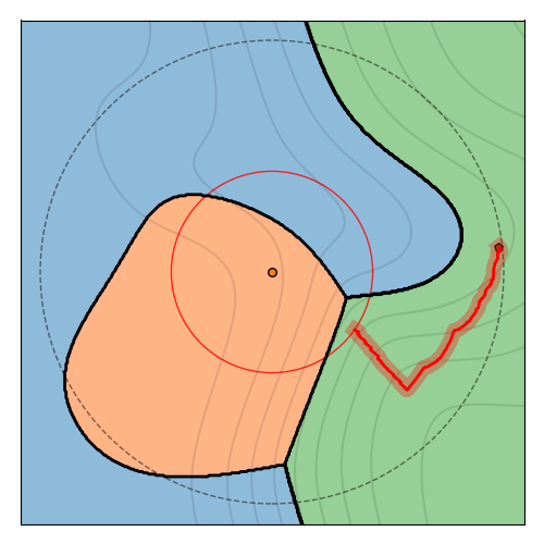
Next, we describe PRISM (partial information substitute model), an approach for targeted evasion technique that combines strengths we identified in Ens and QO. We start by providing an illustration of PRISM in Figure 4. Conceptually, PRISM is similar to QO in Figure 3: it starts the evasion process with image $x_{\rm start}$ of the target class $y^{\prime}$ (Equation 6) and finishes when it finds a solution that is within an $\epsilon$-distance to goal image $x_{goal}$ (Equation 7). Initially, $x_{\rm start}$ is at distance $\left\lVert x_{\rm start}-x_{\rm goal}\right\rVert_{\infty}=d\gg\epsilon$ The method consists of several iterations of increasing the classification likelihood of the j-th iteration $x_{\rm adv}^{j}$ by stepping in the direction of the approximated gradient $\hat{\texttt{G}}_{\texttt{dnn}^{\prime}}$ and then projecting it closer to $x_{\rm goal}$. The procedure continues until the distance between $x_{\rm adv}^{j}$ and $x$ decreases to $\epsilon$, and $x_{\rm adv}$ is classified as the target class $y^{\prime}$ by $\texttt{API}^{\prime}_{\rm k=1}$ or until a query budget $B$ has been exceeded. Although the process of finding $x_{\rm adv}$ is similar to QO (Ilyas et al., 2018b), the gradient estimator comes via substitute model ensembles and MIFGSM as is done in Ens (Dong et al., 2018). We detail pseudocode for PRISM in Algorithm 1.

Figure 4. Decision boundaries of an MLP classifier (3 classes). Targeted evasion with PRISM, starting from start and gradually approaching goal at origin. Maximum modification $\epsilon$ indicated with a red square. Toy example: perturbations bounded with an $L_{2}$-norm.

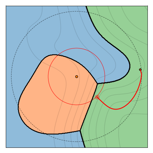
The following steps highlight the differences between PRISM and QO algorithms:

1. We set $\hat{\texttt{G}}_{\texttt{dnn}^{\prime}}(x)\leftarrow\text{ {Ens}}(x)$ in PRISM, which comes from the ensemble models and therefore does not consume queries. With default settings, QO uses 100 queries to determine $\hat{\texttt{G}}_{\texttt{dnn}^{\prime}}(x)$ via finite-difference methods.

2. QO uses line search (Murphy, 2012) to find an appropriate step size with the purpose of reducing queries. PRISM does not do this, since no queries are used.

3. Since PRISM relies on gradient estimates from substitute models, we can aggressively avoid using queries until $d$ has reached $\epsilon$. QO cannot do this, as it needs to remain inside the top-k region in order to calculate gradients.

Algorithm 1 PRISM attack technique

0:  Target $\texttt{API}_{\rm k}(x^{\prime})$, goal image $x_{\rm goal}$, targeted class $y^{\prime}$, starting image of target class $x_{\rm start}$, gradient estimator $\hat{\texttt{G}}(x^{\prime})$, goal $L_{\infty}$-distance $\epsilon\leftarrow 0.05$, patience $C\leftarrow 5$, update threshold $t_{adv}\leftarrow 20\%$, initial $L_{\infty}$-distance limit $d\leftarrow 0.50$, $\delta_{\epsilon}\leftarrow 0.005$.

  

   $x^{\prime}\leftarrow\textrm{Clip}(x^{\prime},x_{\rm start}-d,x_{\rm start}+d)$

  while $d>\epsilon$ and $\texttt{API}_{\mathcal{L}}(x_{\rm adv})\neq y^{\prime}$ do

      $g^{\prime}\leftarrow\hat{\texttt{G}}(x^{\prime})$ {gradient estimation}

      $x^{\prime}\leftarrow x_{\rm adv}+\eta\cdot sign(g^{\prime})$.

      $x^{\prime}\leftarrow\textrm{Clip}(x^{\prime},x_{\rm goal}-d,x_{\rm goal}+d)$.

     if $d=\epsilon$ then

        topk $\leftarrow\texttt{API}_{\rm k}(x^{\prime})$.

     else

         topk $\leftarrow[y^{\prime}]$. {Pseudolabel until $d\leftarrow\epsilon$}

     end if

     if $y^{\prime}\in$ topk then

         $x_{\rm adv}\leftarrow x^{\prime}$

        if  topk$[y^{\prime}]$ $\geq t_{adv}$ then

            $x_{\rm backtrack}\leftarrow x_{\rm adv}$ {update high-confidence $x^{\prime}$}

        end if

        $d\leftarrow max(\epsilon,\epsilon-\delta_{\epsilon})$

     else

         $c\leftarrow c+1$

        if $c>C$  then

            $x_{\rm adv}\leftarrow x_{\rm backtrack}$

        end if

     end if

  end while

It is important to note that PRISM succeeds only as long as Relation 5 holds. For this, we calculate $\hat{\texttt{G}}_{\texttt{dnn}^{\prime}}$ using a large ensemble (approximately 10 models). We further define PRISM_R as a variant of PRISM, with an emphasis on diversity. Instead of always using the same ensemble for gradient estimation like in PRISM, PRISM_R subsamples a random number of ensembles and calculates the gradient with these ensembles using Ens method.

4. Evaluation

4.1. Experimental setup

We first describe our experimental setup, target models and black-box evasion methods. We take the 100 examples from ImageNet as our initial images. These images were used in prior research (Liu et al., 2016), where they were chosen randomly from the ImageNet validation set, such that they were classified correctly by all models in their experiments. We use these images as $x_{\rm goal}$. Our adversary model also specifies $x_{\rm start}$. Since the dataset (Liu et al., 2016) does not consider the partial information setting, we choose $x_{\rm goal}$, $x_{\rm start}$ and target class $y^{\prime}$ from this dataset according to Algorithm 2. We use this setup for all 100 experiments.

Algorithm 2 Experiment Setup

0:  dataset $\mathcal{D}$ with 100 entries $e_{\rm i}$, each entry in format $e_{\rm i}=(x_{\rm i},c_{\rm i})$, where $x_{\rm i}$ refers to an image, and $c_{\rm i}$ is the assigned class

  for $i\leftarrow 0$ to $100$ do

     $x_{\rm goal}\leftarrow x_{\rm i}$

     $x_{\rm start}\leftarrow x_{\rm i+1\text{ mod }100}$

     $y^{\prime}\leftarrow c_{i+1\text{ mod }100}$

  end for

We use the classifiers defined in Table 1 in our evaluation. All classifiers process input of the size $[0,1]^{3\times 224\times 224}$, apart from Inception v3, which processes input of size $[0,1]^{3\times 299\times 299}$. Further, all classifiers expect input to be normalized with RGB color-channel means $(0.485,0.456,0.406)$ and standard deviations $(0.229,0.224,0.225)$, whereas Inception v3 expects input to be normalized to range $[0,1]$ in all color channels. We re-normalize data to the correct range before processing it each classifier, and ensure that images are of correct size with bilinear interpolation.

Table 1. Shorthand notation for DNNs.

	Classifier name (acronym)	Input size
1	SqueezeNet 1.0 (SN1.0) (Iandola et al., 2016)	224
2	SqueezeNet 1.1 (SN1.1) (Iandola et al., 2016)	224
3	ResNet-18 (RN18) (He et al., 2016)	224
4	ResNet-34 (RN34) (He et al., 2016)	224
5	ResNet-50 (RN50) (He et al., 2016)	224
6	DenseNet-121 (DN121) (Huang et al., 2017)	224
7	DenseNet-169 (DN169) (Huang et al., 2017)	224
8	DenseNet-201 (DN201) (Huang et al., 2017)	224
9	VGG11 (Simonyan and Zisserman, 2014)	224
10	VGG16 (Simonyan and Zisserman, 2014)	224
11	ResNet-101 (RN101) (He et al., 2016)	224
12	ResNet-152 (RN152) (He et al., 2016)	224
13	Inception v3 (IncV3) (Szegedy et al., 2016)	299

We define our target APIs and substitute model ensembles in Table 2. For target APIs, we chose Inception v3, ResNet-101, ResNet-152 and VGG16 to experiment with different architecture choices having a low error rate in ImageNet examples. The choice for ensemble components is also shown in Table 2. We choose to divide the target models and ensemble models in this way to study the effect of PRISM between similar architectures (ResNet models, VGG models) and different architectures (Inception as target model). We also formulate target models as $\texttt{API}^{\prime}_{\rm k=1}$, i.e the attacker can only obtain top-1 output from the target model. The ensemble components were chosen with the principle of adding components of different architecture families (SqueezeNet, ResNet, VGG, DenseNet) until the graphics card memory (GeForce 1060, 6GB) was filled. While we could have an even created a stronger adversary by loading additional models in RAM, we found that this represented a reasonably strong and efficient adversary.

Table 2. Ensemble models and target API used in this work. Shorthand notation from Table 1.

Target	Ensemble components
IncV3	Models 1–10
RN101	Models 1–10
VGG16	Models 1–9, 11
RN152	Models 1–11

We investigate the methods shown in Table 3 in this work. Methods 1 (Ens) (Dong et al., 2018) and 4 (QO) (Ilyas et al., 2018b) are state-of-the-art methods among black-box transferable evasion methods, and FDM attacks on partial information APIs, respectively. We investigate how well Ens can reach eventual success, by continuing to query API until a specified query budget is exceeded or success is encountered. Additionally, two variants are investigated. PRISM is a straightforward adaptation of Ens for the setting where $x_{\rm start}\neq x_{\rm goal}$. PRISM_R is a variant of PRISM, using random subsets of the ensemble. We set the query limit to 100,000 queries for QO, and 1,000 for methods Ens, PRISM and PRISM_R after a preliminary investigation. To ensure consistency, all methods are evaluated with PyTorch. We imported the code for QO from the authors’ TensorFlow repository with default parameters. Methods Ens, PRISM and PRISM_R use MIFGSM with the suggested momentum parameter $\mu=1$ and are evaluated with the same ensembles. We evaluate adversarial examples with maximum perturbation $\left\lVert x_{\rm adv}-x_{\rm goal}\right\rVert_{\infty}\leq\epsilon=0.05$, and step size $0.005$ (in Ens, PRISM and PRISM_R), meaning that at least 10 MIFGSM steps are taking before querying the API for the first time. Methods Ens, PRISM and PRISM_R start querying target APIs only after reaching this perturbation. To make results comparable, we assume no knowledge of the resizing operator on each target API. Instead, black-box attacker $\mathcal{A}_{\rm Bbox}$ produces input of the size $[0,1]^{3\times 224\times 224}$ in all methods.

Table 3. Evasion methods. Methods 1–3 use substitute model ensembles from Table 2, while Method 4’s formulation does not make use of substitute models. Method 1 starts adversarial example creation from the goal image $x_{\rm goal}$, while Methods 2–4 have separate goal images and start images.

	Method	Grad. est. $\mathbf{\hat{\texttt{G}}_{\rm dnn^{\prime}}}$	Start class of $x_{\rm start}$
1	Ens	MIFGSM (Dong et al., 2018), full ens.	$\texttt{API}_{\mathcal{L}}^{\prime}(x_{\rm goal})$
2	PRISM	MIFGSM (Dong et al., 2018), full ens.	$y^{\prime}$
3	PRISMR	MIFGSM (Dong et al., 2018), subset ens.	$y^{\prime}$
4	QO	NES (Wierstra et al., 2008)	$y^{\prime}$

4.2. Evaluation criteria

We next define criteria that we use to compare evasion methods.

Success:

A boolean value denoting whether a targeted adversarial example $x_{\rm adv}$ created by method $m_{i}$, for $\texttt{API}^{\prime}$ such that $y^{\prime}\leftarrow\texttt{API}^{\prime}(x_{\rm adv})$, using at most $B$ queries. Success rate refers to how often success occurred in an experiment.

Pareto-efficiency:

given certain evasion setting s, a set of methods $\{m_{1},\dots,m_{L}\}$ and a criteria metric $q(x_{\rm start},x_{\rm goal},y^{\prime},\texttt{API}^{\prime},m_{i})=q(\texttt{s},m_{i})$, a method $m_{i}$ is said to be pareto-efficient for setting s if

(8) $$q(\texttt{s},m_{i})\leq q(\texttt{s},m_{j})~{}\forall i,j\in{1,\dots,L},i\neq j,$$

i.e. $m_{i}$ produces the smallest criteria metric $q$ for setting s. Pareto-efficiency is a descriptive property: given an experiment, we may calculate this statistic in hindsight.

Dominance:

a method $m_{i*}$ is said to dominate other methods in a range $q\in[a,b]$ if

(9) $$\begin{split}\text{E}(q(\texttt{s},m_{i*}))<&\text{E}(q(\texttt{s},m_{j}))~{}\forall{i*},j\in{1,\dots,L},{i*}\neq j\\ q*&=\min_{i}q(\texttt{s},m_{i})~{}\forall i\in\{1,\dots,L\}\\ q*&\in[a,b],\end{split}$$

where $\text{E}(\cdot)$ is the expectation operator, i.e. we expect that $m_{i*}$ will produce the smallest performance metric, given that the pareto-efficient choice produces a metric in the range $[a,b]$. We consider the performance criteria q* in this paper. q* is the minimum number of queries to API’ it requires to produce an adversarial example that is classified as class $y^{\prime}$ on API’ given setup $s$. Dominance is a predictive property: given previous tests, we may extrapolate future performance.

4.3. Baseline evaluations and basic agility

Table 4. Effectiveness of baseline black-box evasion methods Ens and QO, and an agile adversary EQ. Success rate and average number of queries required for success.

	One query	Up to 100,000 queries
	Ens	QO	EQ
IncV3	12% : 1	88% : 44158	89%: 40029
RN101	47%: 1	89%: 32864	96%: 18874
VGG16	47%: 1	94%: 28875	94%: 17433
RN152	58%: 1	91%: 34689	95%: 14754

We first evaluate the baseline methods Ens and QO and how an agile adversary can simply increase efficiency and effectiveness. We show these results in Table 4. The success rate of Ens on the first try is shown in the leftmost column (up to 58% on RN152). The success rate on IncV3 is only 12%. We attribute this to the resize operator in IncV3, which resizes input from $(3\times 224\times 224)$ to $(3\times 299\times 299)$ (cf. Table 1). For example, Xie et al. (Xie et al., 2018) too found that resizing and cropping operations can act as a form of defense against adversarial examples.

On the other extreme, QO reaches approximately 90% success rate on all target APIs with up to 100,000 queries. QO takes between 28,000 and 44,000 queries in average to succeed.

We argue that the pareto-efficient choice for $\mathcal{A}_{\rm Bbox}$ is to switch from one method to another when it becomes apparent that the first method will not succeed. Such an agile adversary can combine the previous methods: after the first query, is done through Ens, the remaining 99,999 queries can be done with QO. We call this simple agile method EQ. We see in Table 4 that the success rate for EQ is between 0–7 percentage points higher than with QO only. In these cases, Ens efficiently (1 query) finds an adversarial example that QO fails at. This occurs especially on RN101 and RN152. We suspect this occurs due to similarity of some of the ensemble components (Table 2). EQ can decrease the average queries between 42 – 58 % on RN101, VGG16 and RN152, i.e. models where Ens produces satisfactory transferability.

4.4. PRISM effectiveness

Table 5. Effectiveness of black-box evasion methods, success rate and median number of queries required for success.

	Up to 1000 queries
	Ens	PRISM	PRISMR	QO
IncV3	26%: 2	69%: 11	75%: 14	0%: -
RN101	83%: 1	88%: 8	93%: 12	0%: -
VGG16	82%: 1	89%: 10	90%: 13	0%: -
RN152	84%: 1	95%: 8	96%: 11	0%: -

Next we evaluate variants of PRISM and compare them to the baseline methods. We show success statistics for each of these four methods in Table 5, given our experimental setup and a query budget of 1000 queries. Columns are arranged in the order of methods presented in Table 3. Columns 1 – 3 represent query use with substitute models, which we advocate in this paper. If we continue querying for up to 1000 times Ens reaches a high success rate on RN101, VGG16 and RN152 (between 82% – 84%). However, Ens success with 1000 queries on IncV3 is significantly lower: only 26%. PRISM and PRISM_R reach 69% and 75% success rates respectively on IncV3, while limited to the same query budget as Ens. By comparison, QO does not reach success since the query budget is too low.

By comparing Tables 4 and 5, we see that the success rate of PRISM_R is in fact very similar as QO on RN101, VGG16 and RN152, while for most of the cases requiring 3 orders of magnitude fewer queries. We also see that in most cases, methods that enable higher success rate do this at the expense of a higher number of median queries. This motivates us to study the comparative effectiveness of different methods. Knowledge of such patterns can help in developing more efficient agile attacks than the one presented in Section 4.3.

4.5. Pareto-efficiency of methods

(a) Inception v3

(b) ResNet-101

(c) VGG16

(d) Inception v3

(e) ResNet-101

(f) VGG16

Figure 5. Subfigures 5(a) – 5(c) illustrate pareto-efficiency of Ens (light blue dot), and QO (light green square), PRISM (dark blue down-pointing triangle) and PRISM_R (dark green up-pointing triangle), evaluated against number of queries required to generate an adversarial example against three models: IncV3, RN101 and VGG16. Subfigures 5(d) – 5(f) illustrate dominance regions. Dominance is calculated as per Equation 9 and illustrates the most effective methods given a certain query region. The thick lines illustrate when methods are optimal and the confidence of that optimality.

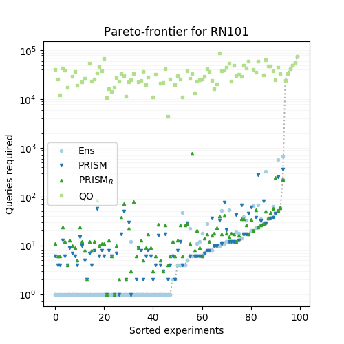
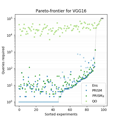
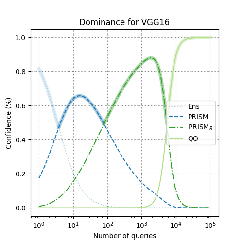
We show the query efficiency of the four methods in Figures 5(a) to 5(c) on IncV3, RN101 and VGG16. The results are sorted so that the examples that required the least number of queries are ordered to the left side. We see that some of the examples are significantly harder than others (positive trend across colors). The most effective methods are connected by a grey dotted line, denoting the pareto-efficient choices. We also see a progression that the most efficient methods on the left side do not work efficiently on the right side. It is harder to find adversarial examples in some experiments than others: by this we mean that the minimum number of queries required to create adversarial examples are bigger than in others. This hints at an inherent exploration-exploitation trade-off: methods that are the most efficient find the universally easy solutions quickly (good exploitation), but tend to underperform on more difficult tasks (poor exploration).

4.6. Dominance and efficient strategies

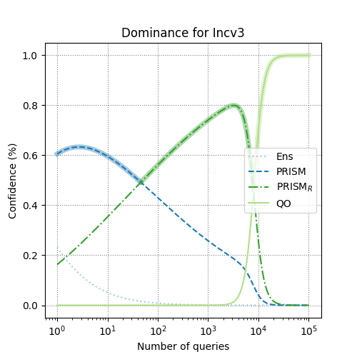
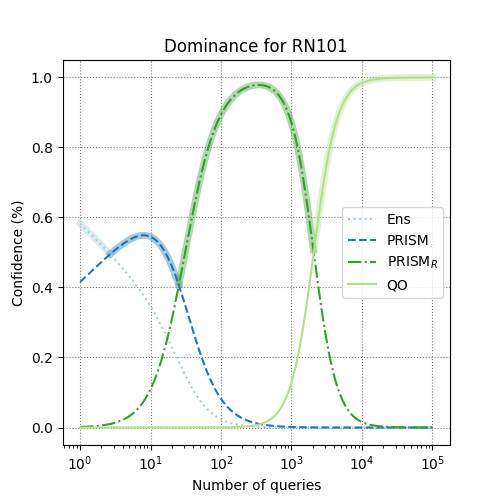
Factoring out the trivial case of transferability, we may ask what is the optimal evasion method, given a certain “hardness” of the task. Using the data points in the previous figure, we can predict which method performs best given a certain region of required queries. Dominance (Equation 9) can be the treated as a multiclass classification problem: finding the most efficient evasion method, given a certain region of required queries. We solve the problem with multinomial logistic regression. Dominance regions are shown in Figures 5(d) to 5(f), and give hints about when it is sensible to switch evasion algorithms, calculated separately for each target model.

Table 6. Approximate dominance regions of evasion methods in Figures 5(a) to 5(c) on IncV3, RN101 and VGG16.

Ens	PRISM	PRISMR	QO
0–1	1–50	50–1,000	1,000–100,000

We identify approximate dominance regions in Table 6. The results indicate a optimal progression of methods to try out, in the order of 1 to 4. Using this we can calculate several instantiations of efficient attacker strategies, e.g. EPP_RQ tries Ens for the first query, PRISM during queries 2–50, PRISM_R between 51–1000 and the rest with QO. Following this strategy, we calculate that the average number of queries required to create adversarial examples on each target model in Table 7. We compare this strategy to only using EPP_R and the previously presented EQ and QO.

Table 7. Comparison on effectiveness and efficiency of EPP_RQ compared to EPQ, EQ and QO. Column 1 details the success rate and average number of queries for success. Columns 2 – 4 compare this to alternative attacker strategies. Row-wise best results are bolded.

	EPPRQ	Cmp. EPQ	Cmp. EQ	Cmp. QO
IncV3	94%:13477	$\pm$0 pp: 1.12$\times$	-5 pp: 1.97$\times$	-6 pp: 2.27$\times$
RN101	100%:2882	-1 pp: 1.56$\times$	-5 pp: 6.55$\times$	-11 pp:11.40$\times$
VGG16	97%:  3497	$\pm$0 pp: 1.00$\times$	-3 pp: 4.98$\times$	-3 pp: 8.26$\times$
RN152	100%:1419	-1 pp: 1.36$\times$	-5 pp:10.39$\times$	-9 pp:24.43$\times$

EPP_RQ is the most effective strategy. It reaches between 94% – 100% success rate on the evaluated models, which is betwen 3 and 11 points higher than QO alone, while using between 2.27$\times$ and 24.43$\times$ less queries. EPP_RQ is also more efficient than EQ, while being significantly more effective. It is clear that PRISM is helpful towards increasing success rate and reducing queries.

We also compare EPP_RQ to EPQ, to confirm whether PRISM_R has any impact on EPP_RQ. We see that the inclusion of PRISM_R does not impact the success rate, but does impact the average number of queries on RN101 and RN152.

Table 8. Comparison on effectiveness and efficiency of EPP_R compared to EQ and QO. Comparative success rate success rate and average number of queries for success. Row-wise best results are bolded.

	EPPR	Cmp. EQ	QO
IncV3	74%: 107	+14 pp: 387$\times$	+13 pp: 427$\times$
RN101	94%:  30	+1 pp: 667$\times$	-5pp: 1162$\times$
VGG16	91%:  37	+3 pp: 496$\times$	+3 pp: 798$\times$
RN152	98%: 28	-3 pp : 530$\times$	-7 pp: 1246$\times$

We additionally compare an attack strategy that only relies on gradient estimates from substitute model ensembles: EPP_R. We compare this strategy to EQ and QO in Table 8. In one case out of four, EPP_R is most effective, and beats all strategies in efficiency: it uses 2.6–2.8 orders of magnitude fewer queries than the basic agile attack EQ, and 2.6–3.1 orders of magnitude fewer queries than QO.

With these results we wish to highlight that agile attackers can present a realistic threat to prediction APIs. We next discuss the threat that PRISM poses to real-life prediction APIs.

4.7. Applicability to real-life APIs

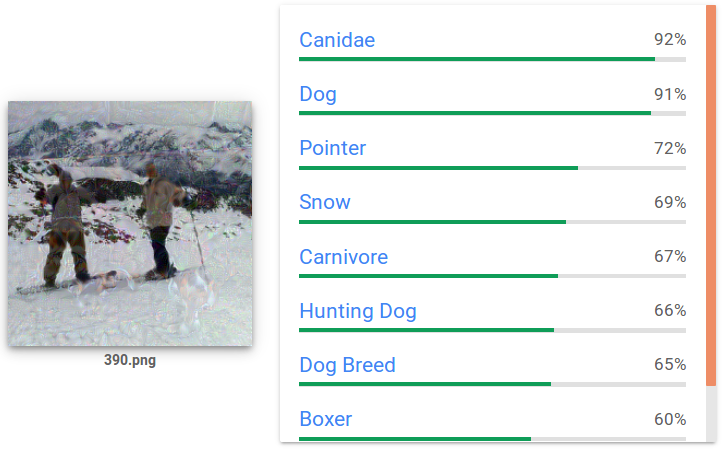
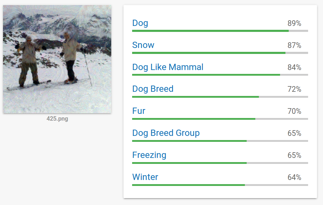
As a proof-of-concept, we tested PRISM against Google Cloud Vision (GCV) API. GCV does not exactly fit our adversary model (Sect. 3.1), as it is trained with non-public data and uses different labels than the substitute models have. This means that the approximation in Relation 5 does not hold well. As we saw in Section 4.5, some setups are harder than others. To provide a comparison with previous techniques, we took the same goal image as in Ilyas et al. (Ilyas et al., 2018b), with the task of changing the image classification of an image with two skiers to “Canidae” (dog-like mammal), and set $\epsilon=0.10$ (as in  (Ilyas et al., 2018b)). However, GCV is under development and becomes more robust to adversarial examples. For example, the original attack example in Ilyas et al. (Ilyas et al., 2018b) does not fool GCV anymore. For the the attack on GCV, we thus relaxed the optimization step S3 (Algorithm 1), and queried all intermediate crafted samples (thus requiring at a minimum 40 queries to go from $d=0.50$ to $d=\epsilon=0.10$ with step size $0.01$).

Nevertheless, we still succeeded. Figure 6 shows the adversarial image that fools GCV in May 2019. The attack required in average 500 queries. However, we found a large difference in the efficiency of our attack between January 2019 and May 2019. In January 2019, we found that approximately 400 queries were enough to fool GCV with modifications of size $\epsilon=5\%$.

Even with 500 queries, the monetary cost of producing adversarial examples can be quite cheap, e.g. with current pricing approximately $0.60 per example. This is small compared to the previous approach by (Ilyas et al., 2018b), which required approximately $26 with current pricing. We estimate that the cost of producing adversarial examples against real-world APIs can be further dropped by judiciously optimizing the use of substitute model ensembles and agile attacks.

Figure 6. Adversarial example by PRISM_R against GCV (May 14th, 2019, $\epsilon=10\%$). Found using 390 queries.

5. Discussion

Next, we study the effect of the size of the ensemble and attack effectiveness. In order to understand the relationship between the number of ensemble components and the effectiveness of substitute model attacks like PRISM and Ens, we calculated the success rate and the median number of queries required for success for different ensemble sizes in Table 9. We increased the number of ensemble components step-by-step from one to ten. We added models from Table 1 to the ensemble in the order of their ImageNet validation set accuracies. As usual, we evaluate adversarial examples with $\epsilon=5\%$.

We make the following observations from Table 9. For a fixed $\epsilon$, we see that adding more components to the ensemble both increases the success rate while decreasing the median number of queries, for all attacks. Adding components is helpful, even when the component itself might have fairly low accuracy (SN1.1 & SN1.0). Table 9 also shows that the effectiveness of the attack increases rapidly when a component with a similar architecture is added to the ensemble (bold font). For example, when attacking VGG16, adding VGG11 to the ensemble increases the success rate from 54% to 85%. We see that PRISM performs better than Ens when several ensemble components are used. We provide intuition as to why PRISM performs better compared to Ens in Appendix A.

Table 9. Ablation study on the size of ensembles for PRISM and Ens. The ensemble size is gradually increased from only one (left) to ten (right). Components with highest top-1 accuracy evaluated first. Success rate and median number of queries for success shown.

Number of components.	1	2	3	4	5	6	7	8	9	10
Target model	IncV3
added model to ens.	DN201	RN101	RN50	DN169	DN121	RN34	RN18	VGG11	SN1.1	SN1.0
Ens (1 query)	2% : 1	4%: 1	5%: 1	6%: 1	6%: 1	8%: 1	10%: 1	12%: 1	12%: 1	12%: 1
Ens (up to 1000 queries)	4% : 9	6%: 1	7%: 1	10%: 1	13%: 2	14%: 1	18%: 1	24%: 1	23%: 1	26%: 2
PRISM (up to 1000 queries)	2%: 89	6%: 60	12%: 28	16%: 27	26%: 14	41%: 15	54%: 12	60% 10	62%: 9	69%: 11
Target model	RN101
added model to ens.	DN201	RN50	DN169	DN121	RN34	VGG16	RN18	VGG11	SN1.1	SN1.0
Ens (1 query)	4%: 1	11%: 1	14%: 1	21%: 1	34%: 1	34%: 1	39%: 1	45%: 1	44%: 1	47%: 1
Ens (up to 1000 queries)	7%: 1	29%: 8	35%: 3	43%: 2	59%: 1	62%: 1	74%: 1	76%: 1	78%: 1	83%: 1
PRISM (up to 1000 queries)	7%: 84	34%: 29	49%: 26	56%: 16	69%: 14	69%: 12	83%: 8	85%: 8	87%: 9	88%: 8
Target model	VGG16
added model to ens.	DN201	RN101	RN50	DN169	DN121	RN34	RN18	VGG11	SN1.1	SN1.0
Ens (1 query)	1%: 1	3%: 1	3%: 1	6%: 1	13%: 1	13%: 1	21%: 1	41%: 1	42%: 1	47%: 1
Ens (up to 1000 queries)	6%: 11	9%: 87	13%: 17	20%: 10	26%: 1	34%: 5	44%: 2	75%: 1	80%: 1	82%: 1
PRISM (up to 1000 queries)	3%: 248	7%: 77	15%: 52	27%: 34	32%: 22	38%: 21	54%: 17	85%: 12	86%: 11	86%: 10

6. Related work

Our paper explored a limited knowledge substitute learner adversary model (Muñoz-González et al., 2017). Other adversary models have also been considered:

Limited knowledge surrogate data:

Tramer et al (Tramèr et al., 2016), Papernot et al (Papernot et al., 2017), Li et al. (Pengcheng et al., 2018) and Juuti et al (Juuti et al., 2019) develop model extraction attacks against DNNs by training a substitute model using synthetic data. Labels are obtained by querying the target model. The substitute model is later used to form transferable adversarial examples.

Model confidentiality:

There have been several attempts (Gilad-Bachrach et al., 2016; Liu et al., 2017; Juvekar et al., 2018) to make the DNNs APIs oblivious, such that the API can process inputs correctly without learning anything about the client’s input, the client simultaneously does not learning anything about the model behind the API.

Other black-box attacks using substitute models:

Wang et al (Wang et al., 2018) explore transfer learning, where a student model for a specific application initialized by a publicly available pretrained teacher model (e.g., Inception v3, VGG16 etc). They show that one can compute adversarial perturbations that can mimic hidden layer representations copied from the teacher in order to fool the student model. They also used ensembles in the case of student model knowledge and an unknown teacher model. They show that their attack performance degrades if several layers of the student models are fine-tuned. Ji et al (Ji et al., 2018) maliciously train pre-trained models in order to implement model-reuse attacks against ML systems without knowing the developer’s dataset or fine-tuning strategies. Hashemi et al (Hashemi et al., 2018) query the target model with images that come from a similar distribution as the training images of the target model, augment the dataset with random noise and use this augmented dataset to train a substitute model. They craft adversarial examples against the substitute model using Carlini & Wagner (Carlini and Wagner, 2017) method and perform transferability attacks. However, for training substitute models, they require logits from the target model in order to mimic decision boundaries and this attack can fail in case of more limited information. Guo et al (Guo et al., 2018) implemented non-differentiable image transformation techniques as a preprocessor in order to defend against black-box and gray-box model evasion attacks. This type of gradient obfuscation techniques are effective when the adversary do not have the knowledge about the preprocessing method.

Finite-difference method attacks:

Similarly to us, Du et al (Du et al., 2018) also consider the partial information attack, and separate between start and goal images. However, they initialize the starting image with a gray color and adopt NES for gradient estimation. They attacked a cloud API (Clarifai food detection) by choosing a valid label from top-k classes and minimizing the probability of so-called non-object or background predictions. Although their gray-image attack requires fewer queries than typical finite-difference methods as in  (Chen et al., 2017; Ilyas et al., 2018b), the adversarial examples are unrecognizable by humans, which is different from our case. Brendel et al (Brendel et al., 2018) introduce a decision-based attack which initializes the starting sample that is already adversarial and walks along the boundary between the adversarial and non-adversarial region as well as decreasing the distance towards the target image. They only used top label for initializing the starting image and finding the direction along the boundary, which is similar to our evaluations, but their attack requires more than an order of magnitude more iterations than the attacks evaluated in this work. Other publications have used gradient-free optimization techniques, such as genetic algorithms (Alzantot et al., 2018) or greedy local search (Narodytska and Kasiviswanathan, 2017) over the image space in order to craft adversarial image in a black-box setting.

7. Conclusions

We presented targeted evasion attacks using substitute model ensembles for black-box APIs. We showed that such attacks can achieve very high effectiveness and efficiency: reaching similar effectiveness as state-of-the-art finite-difference attacks on partial-information APIs, while requiring up to 3 orders of magnitude fewer queries. We showed that the attack relies on the appropriateness of an implicit gradient estimation, and that this gradient approximation benefits from larger substitute model ensembles. Query use with ensembles seems like an interesting direction to explore for future research. As a proof-of-concept, the partial-information formulation of the attack was used to attack Google Cloud Vision, where it succeeded in approximately 400 queries. We argue that query-limited substitute model attacks form a pervasive threat against present-day cloud APIs due to the availability of substitute models and relatively cheap pricing.

Appendix A Appendix

Figure 7 shows an evasion example created by PRISM in January, 2019.

Figure 7. Adversarial example by PRISM against GCV (January 7th, 2019, $\epsilon=5\%$). Found using 425 queries.

(a) $x_{\rm goal}$

(b) $x_{\rm adv}$ found by PRISM

(c) $x_{\rm start}$

Figure 8. An example of an adversarial example $x_{\rm adv}$ found by PRISM, given goal image $x_{\rm goal}$ and start image $x_{\rm start}$. Created against against IncV3 with perturbation $\epsilon=5\%$.

(a) (Closed) linear span of $(x_{\rm start},x_{\rm adv})$ found by PRISM. Confined to range ((-0.1, 0.5), (0. 0.1)). PRISM finds an $x_{\rm adv}$ where a linear interpolation maintains the same classification region as $x_{\rm start}$.

Figure 9. Example of linear spans of $(x_{\rm start},x_{\rm adv})$, starting with the same input, comparing two methods. The sample creation starts in the lower right corner (0.5,0) and progresses towards (0,0). The process ends when the coordinate (0, 0.05) is reached and the sample is still in the same classification region as in $x_{\rm start}$. Evaluated with RN101. Green marks the original class (sea gull), purple the target class (water buffalo) and orange other classes. Contour regions inside the purple region mark logit values of RN101. Red dashed lines mark the path from $x_{\rm start}$ to $x_{\rm adv}$, projected down to the closest point in the linear span of $(x_{\rm start},x_{\rm adv})$, in terms of $L_{1}$-distance. Diagonal lines marks successive 5% absolute increments in $L_{\infty}$-distance: from $x_{\rm start}$. Classification regions sampled with resolution 121x21.

(a) Ens

(b) QO

(c) PRISM

Figure 10. Perturbations of adversarial examples. Created against against IncV3 with perturbation $\epsilon=5\%$.

We show an example of how PRISM evades black-box APIs next. Figure 8 shows a resulting adversarial example, given a goal image and a start image. Figure 9 shows the process of finding the adversarial example with PRISM. The path that PRISM induces is shown in Figure 9(a). Although it is a black-box attack, it essentially follows a hill-climbing route due to the similarity of the gradients of the substitute model and target model. The results in Figure 9(a) suggest that a path between $x_{\rm start}$ and $x_{\rm adv}$ may be found without breaking the classification region of DNNs. The success behind PRISM implies that DNNs have connected but complex classification regions. These results reinforce empirical results by Fawzi et al (Fawzi et al., 2017) who claim that classification regions of DNNs form connected regions, rather than isolated pockets.

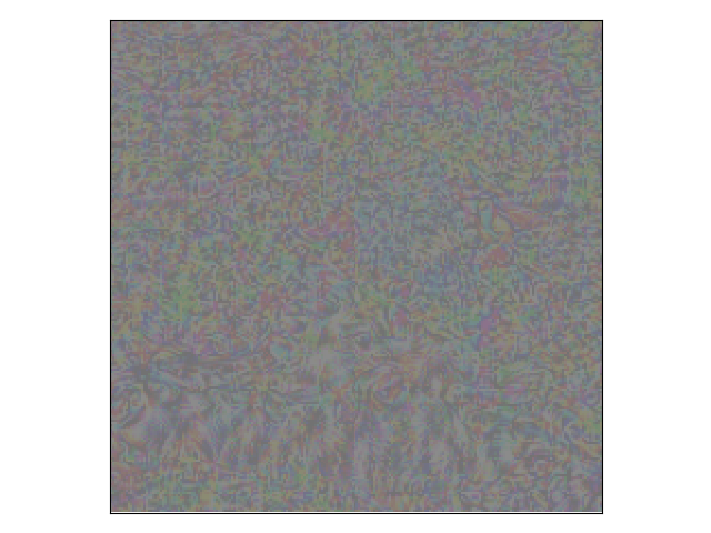
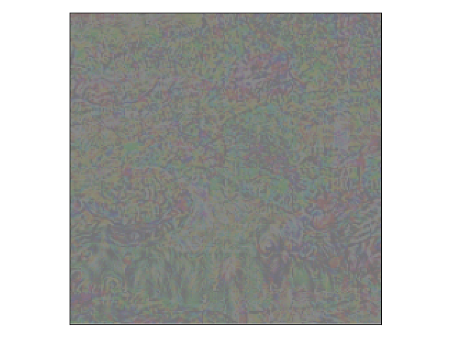
We compare perturbations created by Ens, QO and PRISM in Figure 10, evaluated with IncV3. The goal image and start image are the same as in Figure 8(a) and 8(c). QO perturbations resemble random noise, whereas perturbations created via Ens and PRISM contain regular grid-resembling structures. The perturbation found by PRISM additionally contains localized perturbations influenced from $x_{\rm start}$ (Figure 8(c)), as suggested by Figure 9(a). Note the gradient at the gull wing, greenish tint in background and retained buffalo head.