Applications of Gaussian Binomials to Coding Theory for Deletion Error Correction
Manabu HAGIWARA
Department of Mathematics and Informatics,
Graduate School of Science,
Chiba University
1-33 Yayoi-cho, Inage-ku, Chiba City,
Chiba Pref., JAPAN, 263-0022
Justin KONG
Department of Mathematics,
University of Hawaii at Manoa,
2565 McCarthy Mall (Keller Hall 401A),
Honolulu, Hawaii, U.S.A., 96822
Abstract
We present new applications on -binomials, also
known as Gaussian binomial coefficients.
Our main theorems determine cardinalities
of certain error-correcting codes based on Varshamov-Tenengolts codes
and prove a curious phenomenon relating to deletion sphere for specific cases.
1 Introduction
-binomials [11],
also known as Gaussian
binomial coefficients
[1]
are -analogs of the binomial coefficients.
They are well-known and well-studied, with important
combinatorial implications and have properties
analogous to binomial coefficients
[2, 4, 9, 13].
However, to the best of the authors’ knowledge,
they have not been considered from
the perspective of coding theory for deletion errors.
Terminology is defined precisely in subsequent sections,
but here we give an informal description of the descent
moment distribution. First, a descent vector
(also studied in [7])
is a binary -vector
that indicates the indices of
descent in an associated vector.
The moment of a -vector
(also studied in
[5, 6, 7, 14]) is a
summation of the product of the index
by the value of the -vector.
A descent moment is simply the amalgam of these
two concepts, and the “descent moment distribution”
of a set of vectors is the polynomial whose
coefficients indicate the number of vectors
having a particular descent moment in the given set.
The main contributions of this paper
relate to a class of deletion codes.
This provides implications for calculating the
cardinality of sets that are of interest in the theory of error-correcting codes.
The descent moment distribution in the formula of the main theorem
above is taken over certain sets of interest.
These sets are related to
a well-known class of sets studied by R. P. Stanley
known as VT (Varshamov-Tenengolts) codes [12]
(also known as special cases of Levenshtein codes
[14]).
In his study, Stanley obtained an exact formula for the cardinality of
VT codes by considering a certain moment distribution in
conjunction with the Hamming weight.
The formula was non-trivial, and involved the sum of
Möbius functions and Euler functions.
His formula was for the original VT codes,
but other related sets, in particular permutation and
multi-permutation codes based on VT codes,
do not have such formulas. Moreover, only the moment
distribution was considered, not the descent moment
distribution nor any relation to -binomials.
Partial results were presented at the IEEE International
Symposium on Information Theory (ISIT) 2018 [3].
2 Preliminaries and Remarks
2.1 Descent Moment Distribution
Let be an element of ,
where is a binary ordered set with .
Instead of , the notation is used in this paper.
A 01-vector is called
a descent vector of if
We denote
the descent vector of by .
Sets considered in this paper are often
defined via conditions with descent vectors.
For a 01-vector ,
the moment of is defined as
.
The moment is denoted by .
Note that the moment does not belong to a binary field
but rather it is defined as an integer, whereas is a 01 vector.
For a set of binary sequences,
we introduce the following polynomial of as
our primary interest:
where .
Remark 2.1.
It is easy to see that
The right hand side is well-known
as the major index of .
In this paper, we call the descent moment distribution
for connecting coding theory,
while it is the statistic of major index.
The Hamming weight distribution is an object similar to
[8].
If and
the distribution is
defined as
where is the Hamming weight of ,
i.e., the number of non-zero entries of .
Both distributions may be applied to obtain the cardinality by substituting for their variable:
Another related distribution with both the moment and Hamming weight is:
which is used to obtain the Hamming weight distribution for VT (Varshamov-Tenengolts)
codes (see 2.4 in [12]).
Notice that the descent moment distribution for the union of
disjoint sets is equal to the sum of their descent moment distributions.
Lemma 2.2.
For ,
if ,
Proof.
∎
2.2 -integer, -factorial and -binomial
The notion of a -analogue is a general notion in pure mathematics
for generalizing or extending a mathematical object.
For a mathematical object ,
another mathematical object is called a -analogue
of if or .
For a positive integer ,
the -integer is defined as
and the -factorial is defined as
Using -factorials, for non-negative integers and ,
we define the -binomial as
-binomial is also called a Gaussian binomial coefficient.
It is easy to see that the -integer , the -factorial , and the -binomial
are -analogues of the integer , the factorial , and the binomial respectively.
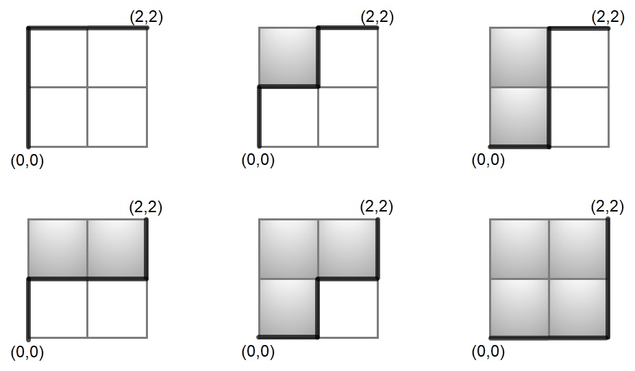
-binomials are known to correlate to certain weight distributions of lattice paths.
Let us consider the set of lattice paths from to .
As is well-known, its cardinality is given by .
By defining the weight of a path as the number of squares
which are on the north-western side of the path,
the following is also well-known [11] (see Example 2.3 below):
Their weights are , , , , , and .
Hence the weight distribution is
On the other hand, the -binomial with and is
The following is used in the proof of Corollary 3.1.
Lemma 2.4.
Let be the th primitive root of
and .
where is the greatest common divisor of and .
Proof.
The assumption implies that ,
and in particular .
The number of zero factors of for substituting to
is and the number of zero factors of is
.
If does not divide ,
it implies .
Hence .
If divides ,
it implies .
Note that
for .
Hence
∎
2.3 Major Index and -binomial
For positive integers and , let be the set of vectors
with entries of and entries of .
Hence consists of elements
that are obtained by all permutations to .
2.4 Coding Theoretic Remarks: Deletions and Partitions via VT Codes
Deletion is a combinatorial operation for a sequence.
Single deletions shorten a given sequence.
For example, a sequence of length changes to the sequence of length
after a single deletion.
Note that a single deletion that occurs in a string of
consecutive repeated entries results in the same sequence
regardless of where the deletion occurs.
Indeed, the deletions in either the 1st entry or the 2nd entry from the sequence
result in the same sequence .
Hence a sequence of length may be changed by a single deletion
to one of three possible sequences of length :
, , or .
For a set of vectors,
we define the set as
the set of sequences
obtained by a single deletion in ,
and call it the deletion sphere of .
For example, for ,
A maximal consecutive subsequence of repetitions of the same entry
is called a run.
For a vector , the number of runs is denoted by
and is called the run number in this paper.
For example, and .
The run number is equal to the number of sequences
that are obtained by single deletions to :
Hence, the cardinality of for a singleton
depends on its element.
A set is called a single deletion correcting code if
This definition is equivalent to
Levenshtein showed that the following sets are single deletion correcting codes for any positive integer and
any integer
[5]:
This code is called a VT code.
The set is written by using VT codes:
The following statement strengthens our motivation to investigate
.
The proof is a direct corollary of Lemma 3.2 in [7].
Theorem 2.10.
The set is a single deletion correcting code.
3 Main Contributions
Our main contributions of this paper are the properties of .
Theorem 3.1
and Corollary 3.2 are enumerative combinatorial results
and
Theorem 3.3
is a coding theoretic result.
3.1 Cardinality of
Theorem 3.1.
For any ,
where is the möbius function, is the Euler function,
and is the greatest common divisor of and .
In particular,
Proof.
Applying Eq. (2), the second half of
Fact 2.5,
we analyze the -binomial
Since the polynomial
is of degree at most ,
is determined by different points of a complex field ,
for example
the elements of the set of th roots of 1.
These two relations above will be used for the proof of
Theorem 3.3.
As preparation, we show the following:
Lemma 3.7.
where denotes the maximal integer that does not exceed .
Proof.
For the sake of brevity, we only show the case when is even. The odd case is similarly proven.
Any element of with runs, where is even, has one of the following two forms:
where () denotes the length of the th run with entry A (B), and
.
For case (*), the descent moment is
and for case (), the descent moment is
Hence
where
,
,
,
and
.
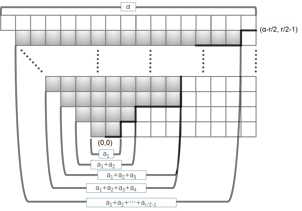
For calculating ,
let us
define a bijection,
depicted by Figure 2,
from the set of sequences
to the set of lattice paths from to .
Note that .
Figure 2: bijection between the set of lattice paths from to
and the set of sequences
Note that in the previous two equations we have used
both and to
represent , which is permissible since is even.
The choices were made so that the end result is consistent
with the case when is odd.
The previous two equations imply that
By a similar argument, we can show
Hence for even ,
As mentioned at the beginning of the proof, the case
when is odd is similarly proven.
∎
The following is the key lemma to prove
Theorem 3.3.
It states that
a sort of symmetry of on holds
by
the assumption and
considering .
In this paper we proved a relationship between
descent moment distributions and -binomials.
To accomplish this, we employed a lattice-path approach
to prove pertinent lemmas.
The relationship between descent moment distributions and
-binomials was then applied to determine the
cardinality of .
We have seen how the descent moment distribution
has some interesting properties and may provide
insights into other problems.
Thus further investigation into descent moment distributions,
especially as it relates to combinatorics,
is a logical future research direction.
Below we state two open questions
regarding the subject.
The natural open question
is to extend the main results of this paper
to ternary (or more) and then arbitrary -multinomials.
That is, the initial part of this open question is to prove a similar relationship
for the descent moment distributions of ternary subsets of
with fixed multiplicities of , , and .
References
[1]
H. Cohn.
Projective geometry over and the gaussian binomial
coefficients.
American Math Monthly, 111(6):487–495, 2004.
[2]
V. Dhand.
A combinatorial proof of strict unimodality for -binomial
coefficients.
Discrete Mathematics, 335:20–24, 2014.
[3]
M. Hagiwara and J. Kong.
Descent moment distributions for permutation deletion codes via
levenshtein codes.
In 2018 IEEE International Symposium on Information Theory
(ISIT), pages 81–85, June 2018.
[4]
T. Kim.
-bernoulli numbers and polynomials associated with gaussian
binomial coefficients.
Russian Journal of mathematical Physics, 15(1):51–57, 2008.
[5]
V.I. Levenshtein.
Binary codes capable of correcting deletions, insertions, and
reversals.
Soviet physics doklady, 10(8):707–710, 1966.
[6]
V.I. Levenshtein.
Asymptotically optimum binary code with correction for losses of one
or two adjacent bits.
Problemy Kibernet, 19:293–298, 1967.
[7]
V.I. Levenshtein.
On perfect codes in deletion and insertion metric.
Discrete Mathematics and Applications, 2(3):241–258, 1992.
[8]
J. MacWilliams.
A theorem on the distribution of weights in a systematic code.
The Bell System Technical Journal, 42(1):79–94, 1963.
[9]
I. Pak and G. Panova.
Strict unimodality of q-binomial coefficients.
Comptes Rendus Mathematique, 351(11-12):415–418, 2013.
[10]
R.P. Stanley.
Enumerative combinatorics. vol. 1, vol. 49 of cambridge studies in
advanced mathematics, 1997.
[12]
R.P. Stanley and M.F. Yoder.
A study of varshamov codes for asymmetric channels.
Jet Prop. Lab. Tech. Rep, pages 32–1526, 1972.
[13]
R.P. Stanley and F. Zanello.
Some asymptotic results on q-binomial coefficients.
Annals of Combinatorics, 20:623–634, 2016.
[14]
G.M. Tenengolts and R.R. Varshamov.
Correction code for single asymmetrical errors(binary code correcting
single asymmetric errors).
Automation and Remote Control, 26:286–290, 1965.