Synthesis and Observation of Non-Abelian Gauge Fields in Real Space

Abstract

Gauge fields, real or synthetic, are crucial for understanding and manipulation of physical systems. The associated geometric phases can be measured, for example, from the Aharonov–Bohm interference. So far, real-space realizations of gauge fields have been limited to Abelian (commutative) ones. Here we report an experimental synthesis of non-Abelian gauge fields in real space and the observation of the non-Abelian Aharonov–Bohm effect with classical waves and classical fluxes. Based on optical mode degeneracy, we break time-reversal symmetry in different manners—via temporal modulation and the Faraday effect—to synthesize tunable non-Abelian gauge fields. The Sagnac interference of two final states, obtained by reversely-ordered path integrals, demonstrates the non-commutativity of the gauge fields. Our work introduces real-space building blocks for non-Abelian gauge fields, relevant for classical and quantum exotic topological phenomena.

Gauge fields are the backbone of gauge theories, the earliest example of which is classical electrodynamics. However, until the seminal Aharonov–Bohm effect Aharonov and Bohm (1959), the scalar and vector potentials of electromagnetic fields have been considered as a convenient mathematical aid, rather than objects carrying physical consequences. It has been realized by Berry Berry (1984) that the Aharonov–Bohm phase imprinted on electrons can be interpreted as a real-space example of geometric phases Berry (1984); Pancharatnam (1956), which in fact appear in versatile physical systems. For charge-neutral particles, such as photons Sounas and Alù (2017); Yuan et al. (2018) and cold atoms Dalibard et al. (2011); Eckardt (2017); Goldman et al. (2014), synthetic gauge fields can be created in real, momentum, or synthetic (i.e. other parameters besides position or momentum) space. These synthetic gauge fields enable engineered, artificial magnetic fields in systems of either broken or invariant time-reversal symmetry; and thus play a pivotal role in the realizations of topological phases Goldman et al. (2014); Lu et al. (2014); Ozawa et al. (2018); Aidelsburger et al. (2018), quantum simulations Bloch et al. (2012); Aspuru-Guzik and Walther (2012), and optoelectronic applications Tzuang et al. (2014); Fang et al. (2017).

Gauge fields are classified into Abelian (commutative) and non-Abelian (non-commutative), depending on the commutativity of the underlying group. Synthetic Abelian gauge fields have been realized in various platforms including cold atoms Lin et al. (2009); Aidelsburger et al. (2011); Miyake et al. (2013); Struck et al. (2012); Aidelsburger et al. (2013, 2015); Jotzu et al. (2014); Ray et al. (2014); Li et al. (2016), photons Fang et al. (2012a, b); Hafezi et al. (2011); Umucalılar and Carusotto (2011); Li et al. (2014); Mittal et al. (2014); Schine et al. (2016); Rechtsman et al. (2013); Haldane and Raghu (2008); Wang et al. (2009), phonons Xiao et al. (2015); Yang et al. (2017); Abbaszadeh et al. (2017), polaritons Lim et al. (2017), and superconducting qubits Schroer et al. (2014); Roushan et al. (2014, 2017). The synthesis of non-Abelian gauge fields is more challenging, due to the requirements of degeneracy and non-commutative, matrix-valued gauge potentials. So far, they have been achieved only in the momentum and synthetic spaces. Specifically, non-Abelian gauge fields have been realized in the momentum space using two-dimensional spin-orbit coupling Huang et al. (2016); Wu et al. (2016) in cold atoms. In the synthetic space, non-Abelian geometric phases Wilczek and Zee (1984); Wilczek and Shapere (1989), initially observed in nuclear magnetic resonances Zwanziger et al. (1990); Zee (1988); Mead (1987, 1992), have enabled non-Abelian geometric gates Abdumalikov Jr et al. (2013) and the simulation of an atomic Yang monopole Sugawa et al. (2018). As yet, however, the realization of non-Abelian gauge fields in real space remains a bottleneck; therefore, the non-Abelian generalization of the Aharonov–Bohm effect—a real-space phenomenon that has stimulated longstanding theoretical interests Wu and Yang (1975); Horváthy (1986); Alford et al. (1990); Chaichian et al. (2002); Osterloh et al. (2005); Jacob et al. (2007); Iadecola et al. (2016); Chen et al. (2018); Dalibard et al. (2011); Bohm et al. (2013)—remains experimentally elusive.

Here we report the observation of the non-Abelian Aharonov–Bohm effect by synthesizing non-Abelian gauge fields in real space. Exploiting a degeneracy in photonic modes, we create non-Abelian gauge fields by cascading multiple non-reciprocal optical elements that break the time-reversal symmetry ($\mathcal{T}$) in orthogonal bases of Hilbert space. We demonstrate the genuine non-Abelian condition of our gauge fields in a fiber-optic Sagnac interferometer. The observed interference patterns show the signature features of the non-commutativity between a pair of time-reversed, cyclic evolution operators. We also demonstrate that our synthetic magnetic fluxes are fully tunable, enabling controlled transitions between the Abelian and the non-Abelian regimes. Taken together, our results lay the groundwork for the synthesis of non-Abelian gauge fields in real space, which provides basic ingredients for studying relevant single- or many-body topological states in photonic platforms.

Synthetic non-Abelian gauge fields demand a degeneracy of levels, which can, for example, be achieved by utilizing the internal degrees of freedom in quantum gases or exploiting the polarization/mode degeneracy and electromagnetic duality in photons. For a particle moving along a closed path in a non-Abelian gauge field, its evolution operator reads $\boldsymbol{W}\equiv\mathcal{P}\exp\mathrm{i}\oint\boldsymbol{A}\mathop{}\mathrm{d}\mathbf{l},$ where $\mathcal{P}$ represents path-ordered integral and $\boldsymbol{A}$ is the matrix-valued gauge field. Its trace, $W\equiv\mathrm{Tr}\,\boldsymbol{W}$, is gauge-invariant, and is also known as the Wilson loop Wilson (1974). For particles with N-fold degeneracies, the non-Abelian gauge fields can take forms of U(N). Here we focus on the SU(2) gauge fields, since our photonic system enables the definition of a pseudospin—a two-fold degeneracy in the polarization states. Crucially, we focus on the situations where the involved gauge fields break $\mathcal{T}$-symmetry and state transport becomes nonreciprocal. In what follows we illustrate the consequence of real-space guage fields on the pseudospin evolution in Hilbert space [i.e. the Poincaré (or Bloch) sphere].

The difference between how a state evolves in Abelian gauge fields versus in non-Abelian gauge fields is shown in Fig. 1. In a uniform Abelian gauge field $\propto\boldsymbol{\sigma}_{z}$, the evolution operator along a closed loop can be simplified as $\boldsymbol{W}=\mathrm{e}^{\mathrm{i}\phi\boldsymbol{\sigma}_{z}}$, where $\boldsymbol{\sigma}_{z}$ is the $z$ component of the Pauli matrices and $\phi$ is the flux of the gauge field through this closed loop (Fig. 1a). Consequently, the state rotates by $2\phi$ around the $z$ axis of the Poincaré sphere (Fig. 1b). If the state evolves along two consecutive closed loops, the two evolution operators are commutative, which reflects the Abelian nature of this gauge field. Similarly, a homogeneous gauge field $\propto\boldsymbol{\sigma}_{y}$ in real space (Fig. 1c) is also Abelian, as the state always evolve around the $y$ axis in the Hilbert space (Fig. 1d).

In contrast, non-Abelian gauge fields require inhomogeneous gauge structures. Fig. 1ef illustrate such an example where two different $\boldsymbol{\sigma}_{z}$ and $\boldsymbol{\sigma}_{y}$ gauge structures are concatenated into one compound closed loop. The same initial state $\boldsymbol{s}_{\mathrm{i}}$ can now evolve into different final states: $\boldsymbol{s}_{\text{f}}^{\theta\phi}$ or $\boldsymbol{s}_{\text{f}}^{\phi\theta}$ (Fig. 1g), depending on the different ordering—$\phi$ and then $\theta$, or alternatively, $\theta$ and then $\phi$—of the two gauge structures. The interference between the two final states $\boldsymbol{s}_{\text{f}}^{\theta\phi}$ and $\boldsymbol{s}_{\text{f}}^{\phi\theta}$ is known as the non-Abelian Aharonov–Bohm effect Wu and Yang (1975); Horváthy (1986); Alford et al. (1990); Chaichian et al. (2002); Iadecola et al. (2016); Chen et al. (2018); Dalibard et al. (2011); Bohm et al. (2013); Jacob et al. (2007); Osterloh et al. (2005). This effect, that we will experimentally demonstrate later, is the most direct manifestation of non-Abelian gauge fields in real space.

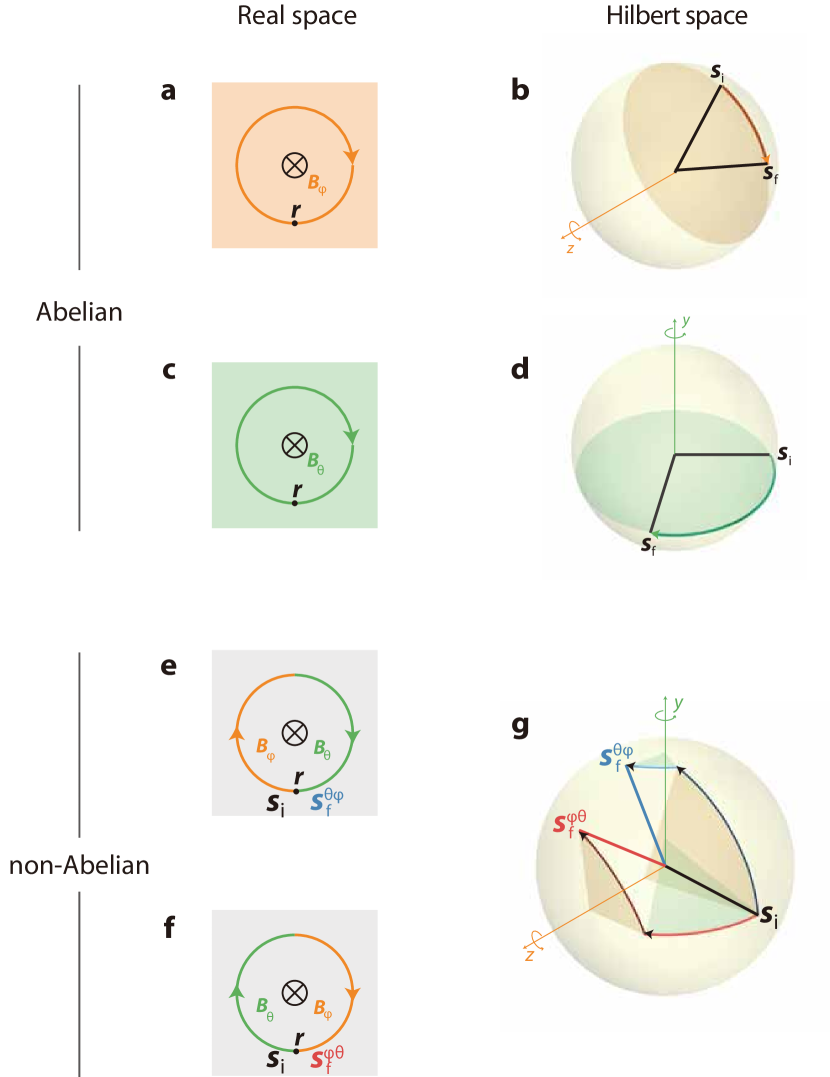
Figure 1: Comparison between SU(2) Abelian and non-Abelian gauge fields in real space and in Hilbert space. a-d. Along a closed loop inside an Abelian gauge field $\boldsymbol{A}\propto\boldsymbol{\sigma}_{z}$ (a) or $\boldsymbol{\sigma}_{y}$ (c), the state evolves by rotating around the $z$ (b) or $y$ (d) axis of the Poincaré sphere. Within each case (a-b or c-d), the state evolution are always commutative. e-f. In non-Abelian gauge fields, the evolution operators for different loops are no longer commutative, which leads to different final states, $\boldsymbol{s}_{\text{f}}^{\theta\phi}$ and $\boldsymbol{s}_{\text{f}}^{\phi\theta}$ , for the same initial state $\boldsymbol{s}_{\text{i}}$. The non-commutativity can be tested by an Aharonov–Bohm interference of the two final states.

In our photonic implementation, we experimentally synthesize the inhomogeneous gauge potentials in a fiber-optic system, which is conceptually illustrated in Fig. 2a. We identify the horizontal and vertical transverse modes (denoted by $\ket{\text{h}}$ and $\ket{\text{v}}$ respectively) in optical fibers as the pseudospin. Crucially, we synthesize two types of gauge fields, $\phi\boldsymbol{\sigma}_{z}$ and $\theta\boldsymbol{\sigma}_{y}$, using two distinct methods to break $\mathcal{T}$-symmetry.

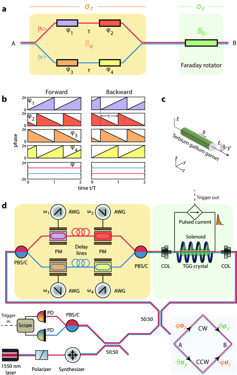
Figure 2: Synthesis of non-Abelian gauge fields. a. Non-Abelian gauge fields for photons. Temporal modulation and the Faraday effect, which break T-symmetry in two orthogonal bases of the Hilbert space, are used to synthesize $\boldsymbol{\sigma}_{z}$ and $\boldsymbol{\sigma}_{y}$ gauge fields, respectively. b. Pseudospin-dependent non-reciprocal phase shifts are created through sawtooth phase modulations, which corresponds a synthetic gauge field along $\boldsymbol{\sigma}_{z}$. c. Non-reciprocal rotation of the pseudospin is achieved via the Faraday effect in a terbium gallium garnet crystal, which corresponds to a synthetic gauge field along $\boldsymbol{\sigma}_{y}$. d. Experimental setup. The interference between different final pseudospin states—originated from reversed ordering of the gauge structures (CW and CCW, inset)—is read out through a Sagnac interferometer, which gives rise to the non-Abelian Aharonov—Bohm effect. PBS/C: polarization beam splitter/combiner; PM: phase modulator; AWG: arbitrary waveform generator; COL: collimator; TGG: Terbium Gallium Garnet; PD: photodetector.

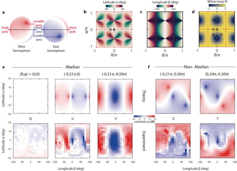
Figure 3: Non-Abelian Aharonov–Bohm interference. a. Contrast function $\rho$ on the Poincaré sphere, featured by a fixed zero/pole pair on the equator, and a tunable zero/pole pair (which indicates the consequence of gauge fluxes). The two pairs of zeros and poles are always antipodal. b-c. Location (latitude and longitude) of the tunable pole on the Poincaré sphere as a function of the gauge fluxes $(\theta,\phi)$. Abelian gauge fields correspond to on-equator poles (red dashed lines); non-Abelian gauge fields correspond to off-equator poles—both of which are experimentally demonstrated. d.  Wilson loops $W$ on the synthetic torus $(\theta,\phi)$. $|W|=2$ (red dashed lines) is a necessary but insufficient condition for non-Abelian guage fields (cf. b) . e-f. Examples of predicted and observed contrast functions $\rho$ for Abelian (Q, U, and V) and non-Abelian (X and Y) gauge fields.

To construct a gauge field of $\phi\boldsymbol{\sigma}_{z}$, we first employ dynamic modulations that dress $\ket{\text{h}}$ and $\ket{\text{v}}$ with nonreciprocal phase shifts of $\pm\phi$, respectively. Specifically, four LiNbO₃ phase modulators—two (labeled 1 and 2) for $\ket{\text{h}}$ and two (labeled 3 and 4) for $\ket{\text{v}}$—are driven by arbitrary waveform generators that create phase shifts in the form of sawtooth functions in time (Fig. 2b). Modulators 1 and 4 are positive in slope: $\phi_{1,4}=\omega t\mod 2\pi$; and modulators 2 and 3 are negative in slope, $\phi_{2,3}=-\omega t\mod 2\pi$. The delay line between modulators 1 and 2 (3 and 4) corresponds to a delay time $\tau$. As a result, besides dynamic phases, $\ket{\text{h}}$ ($\ket{\text{v}}$) picks up an extra phase $\phi=\omega\tau$ ($-\omega\tau$) in the forward (i.e. left-to-right) direction, but an opposite phase $-\phi$ ($+\phi$) in the backward direction. This pair of opposite nonreciprocal phases for opposite pseudospin components ($\ket{\text{h}}$ and $\ket{\text{v}}$) correspond to a $\phi\boldsymbol{\sigma}_{z}$ gauge field, which is continuously tunable by varying the modulation frequency $\omega$.

A second, orthogonal type of gauge field, $\theta\boldsymbol{\sigma}_{y}$, is created using the Faraday effect. Specifically, light is coupled out of the fiber, sent through a Terbium Gallium Garnet crystal placed in an external magnetic field, and then coupled back into the fiber. Through the Faraday effect, pseudospin of light is rotated in a nonreciprocal way, which corresponds to a gauge field of $\theta\boldsymbol{\sigma}_{y}$. This gauge field is also continuously tunable through the external magnetic field.

We then concatenate the two non-Abelian gauge fields to demonstrate the non-Abelian Aharonov–Bohm effect via Sagnac interferometry (inset of Fig. 2d). In such Sagnac configuration, the two sites A and B in Fig. 2a are combined into the same physical location to enable well-defined non-Abelian gauge fluxes. Evolved from the clockwise (CW) and counter-clockwise (CCW) paths of the Sagnac loop, the two final states are $\boldsymbol{s}_{\text{f}}^{\theta\phi}=\boldsymbol{\sigma}_{z}\mathrm{e}^{\mathrm{i}\theta\boldsymbol{\sigma}_{y}}\mathrm{e}^{\mathrm{i}\phi\boldsymbol{\sigma}_{z}}\boldsymbol{s}_{\mathrm{i}}$ and $\boldsymbol{s}_{\text{f}}^{\phi\theta}=\mathrm{e}^{-\mathrm{i}\phi\boldsymbol{\sigma}_{z}}\mathrm{e}^{-\mathrm{i}\theta\boldsymbol{\sigma}_{y}}\boldsymbol{\sigma}_{z}\boldsymbol{s}_{\mathrm{i}}$, where the $\boldsymbol{\sigma}_{z}$ term maintains a consistent handedness of the polarization for counter-propagating states. The interference of the two final states is given by (Sec. S6)

$$\mathbf{s}_{\text{f}}=\boldsymbol{s}_{\text{f}}^{\theta\phi}+\boldsymbol{s}_{\text{f}}^{\phi\theta}=-\boldsymbol{\sigma}_{x}\left(\mathrm{e}^{\mathrm{i}\theta^{\prime}\boldsymbol{\sigma}_{y}}\mathrm{e}^{\mathrm{i}\phi\boldsymbol{\sigma}_{z}}+\mathrm{e}^{\mathrm{i}\phi\boldsymbol{\sigma}_{z}}\mathrm{e}^{\mathrm{i}\theta^{\prime}\boldsymbol{\sigma}_{y}}\right)\boldsymbol{s}_{\mathrm{i}},$$ (1)

where $\theta^{\prime}=\theta+\pi/2$ and $\boldsymbol{\sigma}_{x}$ is a global spin flip. This interference describes a Sagnac-type realization of the non-Abelian Aharonov–Bohm effect Dalibard et al. (2011)—the interference between two final states, which originate from the same initial state, but undergo reversely-ordered, inhomogeneous path integrals (Fig. 1e-g) in the CW and CCW directions.

Fig. 2d details our experimental setup (Sec. S1). We place a polarization synthesizer in front of the Sagnac loop, to prepare any desired pseudospin state as the input in a deterministic manner. After exiting the Sagnac loop, the two final states $\boldsymbol{s}_{\text{f}}^{\theta\phi}$ and $\boldsymbol{s}_{\text{f}}^{\phi\theta}$ interfere with each other. The associated interference intensity is projected onto the horizontal and vertical bases, which are then measured separately. Within the Sagnac loop, a solenoid—driven by tunable pulsed currents (peak current $\approx$ $2\text{\,}\mathrm{kA}$, duration $\approx$ $10\text{\,}\mathrm{ms}$)—provides a magnetic field between 0 and $\approx$ $2\text{\,}\mathrm{T}$ (Sec. S2) for the Faraday rotator. The solenoid also provides a temporal trigger signal for the detection. For the dynamic modulation, we assign four different modulation frequencies (i.e. slopes of the temporal sawtooth functions) $+\omega_{1}$, $-\omega_{2}$, $-\omega_{3}$, and $+\omega_{4}$ to each of the modulators with $\omega_{i}$ defined to be positive. We impose an additional constraint that $\omega\equiv(\omega_{1}+\omega_{2})/2=(\omega_{4}+\omega_{3})/2$. This modified arrangement from Fig. 2b maintains the same nonreciprocal phases and thus the gauge fields $\phi\boldsymbol{\sigma}_{z}$ (Sec. S8). The advantage of this modification is an experimental one: it relocates the relevant interference fringes from zero to a nonzero carrier frequency $\Omega\equiv\omega_{1}-\omega_{2}+\omega_{3}-\omega_{4}$, which is less sensitive to environmental or back-scattering noises.

We next define our experimental observable and explain its relevance to non-Abelian gauge fields. In the original U(1) Abelian Aharonov–Bohm effect, the observable is the interference intensity as a function of the Abelian magnetic flux. In our case, analogously, for each given set of non-Abelian gauge fluxes $(\theta,\phi)$, we measure the contrast $\rho$ between the interference intensities projected onto the horizontal and vertical bases. Specifically, we measure $\rho(\theta,\phi,\alpha,\beta)\equiv I_{\text{h}}^{\Omega}/I_{\text{v}}^{\Omega}$, where $(\alpha,\beta)$ are the latitude and longitude of the input pseudospin state on the Poincaré sphere and $I_{\text{h(v)}}^{\Omega}$ is the intensity of $\ket{\text{h}}$ and $\ket{\text{v}}$ component of the output pseudospin state at the carrier frequency $\Omega$, respectively. Therefore, $\rho$ is defined on a manifold of $S^{2}\times T^{2}$, which is spanned by the Hilbert space of the input pseudospin $S^{2}$ and the synthetic space of the gauge fluxes ($\theta$, $\phi$) that is $T^{2}$.

For a fixed set of magnetic fluxes $(\theta,\phi)$, the contrast function $\rho(\alpha,\beta)$ always exhibits two pairs of first-order zeros and poles on the Poincaré sphere (Fig. 3a; also see Sec. S9). Within each pair, the zero and the pole are always antipodal and thus represent orthogonal pseudospins. One pair, being linear polarizations $(1,0)$ (zero) and $(0,1)$ (pole), is fixed on the two ends of the equator, regardless of the choice of $(\theta,\phi$). The other orthogonal pesudospin pair, however, is tunable on the entire sphere via the synthetic gauge fluxes $(\theta,\phi)$. These zeros and poles are conserved quantities on the Poincaré sphere and dictate the behavior of the contrast $\rho$ function. Their generation, evolution, and annihilation are directly related to the transitions between the Abelian and non-Abelian regimes. Fig. 3bc show the latitude $\alpha$ and longitude $\beta$ of the tunable pole on the Poincaré sphere, as a function of magnetic fluxes $(\theta,\phi)$. When $\theta=m\pi/2$ or $\phi=n\pi/2$ ($m$ and $n$ are integers), the tunable zero-pole pair appears on the equator (red dashed lines in Fig. 3b). This key feature—an on/off-equator zero/pole—can be used to straightforwardly differentiate between Abelian and non-Abelian gauge fields synthesized in our experiment (see Fig. 3ef).

The necessary and sufficient condition for gauge fields to be non-Abelian is as follows. There exists two loop operators, $\boldsymbol{W}_{1}$ and $\boldsymbol{W}_{2}$, both starting and ending at the same site in space, such that they are non-commutative, i.e. $\boldsymbol{W}_{1}\boldsymbol{W}_{2}\neq\boldsymbol{W}_{2}\boldsymbol{W}_{1}$ Goldman et al. (2014). In an Aharonov–Bohm interference, whether Abelian or non-Abelian, $\boldsymbol{W}_{1}$ and $\boldsymbol{W}_{2}$ can be identified as a pair of time-reversal partners that share the same physical path. We first examine $\boldsymbol{W}_{1}=l_{\text{b}}^{-1}\cdot l_{\text{t}}$ and $\boldsymbol{W}_{2}=l_{\text{t}}^{-1}\cdot l_{\text{b}}$ in the Abelian Aharonov–Bohm experiment, whose two distinct top and bottom paths are denoted by $l_{\text{t}}$ and $l_{\text{b}}$, respectively. Under time-reversal, both momentum and vector potential flip sign, rendering $\boldsymbol{W}_{1}=\boldsymbol{W}_{2}=\mathrm{e}^{\mathrm{i}\gamma}$ that are clearly commutative and exhibit identical, scalar Berry phases $\gamma$ (Sec. S7.A). In our non-Abelian Aharonov–Bohm experiment, the time-reversal pair $\boldsymbol{W}_{1}$ and $\boldsymbol{W}_{2}$ can be analogously defined by replacing $l_{\text{t}}$ and $l_{\text{b}}$ with CW and CCW paths (Fig. 2d inset), which yields (Sec. S7.A)

$$\boldsymbol{W}_{1} =\mathcal{P}\exp\mathrm{i}\oint_{\text{CCW}^{-1}\cdot\text{CW}}\boldsymbol{A}\mathop{}\mathrm{d}{\boldsymbol{l}}=\boldsymbol{\sigma}_{z}\mathrm{e}^{\mathrm{i}\theta\boldsymbol{\sigma}_{y}}\mathrm{e}^{\mathrm{i}\phi\boldsymbol{\sigma}_{z}}\boldsymbol{\sigma}_{z}\mathrm{e}^{\mathrm{i}\theta\boldsymbol{\sigma}_{y}}\mathrm{e}^{\mathrm{i}\phi\boldsymbol{\sigma}_{z}},$$ (2)

$$\boldsymbol{W}_{2} =\mathcal{P}\exp\mathrm{i}\oint_{\text{CW}^{-1}\cdot\text{CCW}}\!\!\!\!-\boldsymbol{A}\mathop{}\mathrm{d}{\boldsymbol{l}}=\mathrm{e}^{\mathrm{i}\phi\boldsymbol{\sigma}_{z}}\mathrm{e}^{\mathrm{i}\theta\boldsymbol{\sigma}_{y}}\boldsymbol{\sigma}_{z}\mathrm{e}^{\mathrm{i}\phi\boldsymbol{\sigma}_{z}}\mathrm{e}^{\mathrm{i}\theta\boldsymbol{\sigma}_{y}}\boldsymbol{\sigma}_{z}.$$ (3)

The condition for $\boldsymbol{W}_{1}$ and $\boldsymbol{W}_{2}$ to be non-commutative is satisfied when $\theta\neq m\pi/2$ and $\phi\neq n\pi/2$ (Sec. S7.A)—the same condition also guarantees the existence of a zero and a pole of the contrast function away from the equator (Fig. 3b). $\boldsymbol{W}_{1}$ and $\boldsymbol{W}_{2}$ are also connected via a unitary gauge transformation (Sec. S7.A); therefore they always share the same Wilson loop (Sec. S7.C) $W=\mathrm{Tr}\,\boldsymbol{W}_{1}=\mathrm{Tr}\,\boldsymbol{W}_{2}=2-4\cos^{2}\theta\sin^{2}\phi.$ Fig. 3d shows this Wilison loop on the $T^{2}$ space of gauge fluxes. Generally speaking, in an $N$-fold degenerate system, $|W|=N$ means the state evolution can be trivially understood by decoupling the system into the product of $N$ Abelian subsystems Goldman et al. (2014). In our case, such trivial configurations are shown with red dashed lines [$\theta=(m+1/2)\pi$, $\phi=n\pi$, or $\theta=m\pi$ and $\phi=(n+1/2)\pi$] in Fig. 3d. Nevertheless, $|W|\neq N$ is only a necessary but insufficient condition for gauge fields to be non-Abelian Goldman et al. (2014), as evident from the comparison between Fig. 3b and Fig. 3d: some configurations with $|W|\neq N$ are still Abelian.

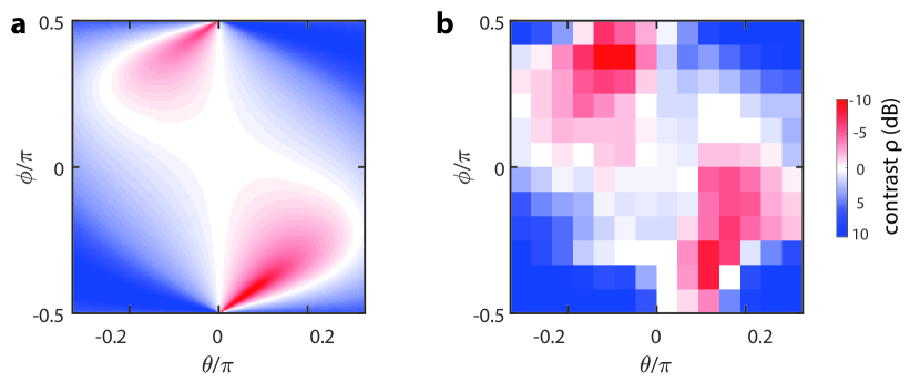
Figure 4: Tunability of the non-Abelian gauge fields. Predicted (a) and measured (b) contrast function $\rho$ for a fixed incident pseudospin state $(\alpha,\beta)\approx(-51\degree,-12\degree)$. The gauge fields $\phi\boldsymbol{\sigma}_{z}$ and $\theta\boldsymbol{\sigma}_{y}$ are continuously tuned by respectively varying the modulation frequencies in the arbitrary waveform generators and the voltages applied to the solenoid.

In Fig. 3ef, we characterize our synthetic gauge fields by measuring the contrast function $\rho$. We present the comparison between theoretical predictions (top row) and experimental measurements (bottom row) for five sampling points on the synthetic space $T^{2}$: Q, U, V are Abelian; and X, Y are non-Abelian. In the Abelian case Q [$(\theta,\phi)\approx(0,0)$], the tunable pole and the fixed zero annihilate each other at $(\alpha,\beta)=(0\degree,0\degree)$; so do the tunable zero and the fixed pole at $(\alpha,\beta)=(0\degree,180\degree)$. As a result, the contrast remains a constant $\rho=1$ regardless of the input pseudospin state. This is a direct consequence of the preserved $\mathcal{T}$-symmetry in the absence of gauge fluxes. In case U [$(\theta,\phi)\approx(-0.21\pi,0)$], the annihilation of poles with zeros are lifted; nevertheless, both poles and zeros appear on the equator, and the gauge structure remains Abelian, since we only break $\mathcal{T}$-symmetry once. In case V [$(\theta,\phi)\approx(-0.21\pi,0.50\pi)$], which is still Abelian, the two poles (zeros) coalesce and produce a second-order pole (zero) on the equator. In cases X [$(\theta,\phi)\approx(-0.21\pi,-0.30\pi)$] and Y [$(\theta,\phi)\approx(0.24\pi,-0.30\pi)$], our synthesized gauge fields become non-Abelian, as indicated by the observed off-equator zeros and poles. For all the cases, our observations show agreement with the associated predictions. In our interferometer, the two spin basis $\ket{\text{h}}$ and $\ket{\text{v}}$, are not perfectly degenerate due to the difference in their refractive indices ($\sim 10^{-4}$). This difference leads to a reciprocal, linear birefringent phase (i.e. a dynamic phase contribution), which is calibrated and consistently applied to all measurements (Sec. S4).

Up to this point, we have measured the contrast $\rho$ for fixed gauge fluxes, while changing the input states. In a complementary manner, we can now fix the input state $(\alpha,\beta)$ and demonstrate the tunability of the synthesized non-Abelian gauge fields by measuring the contrast $\rho$ for different synthetic gauge fluxes $(\theta,\phi)$. As shown in Fig. 4, we reach similar agreeement between the theoretical prediction and the measurement.

In summary, we demonstrate an experimental synthesis of non-Abelian gauge fields in the real space, which is confirmed by our observation of the non-Abelian Aharonov—Bohm effect using classical particles and classical fluxes. The realized gauge fields demonstrate a viable way to engineer the Peierls phase in the simulation of topological systems, such as the non-Abelian Hofstadter models Osterloh et al. (2005); Goldman et al. (2009) (also see Sec. S10). Our experiment also introduces non-Abelian ingredients for realizing high-order topological phases Benalcazar et al. (2017); Peterson et al. (2018); Serra-Garcia et al. (2018) and topological pumps Zilberberg et al. (2018); Lohse et al. (2018). Besides, recent advances in on-chip modulation Wang et al. (2018) and magneto-optical materials Bi (2018) could enable future observations of non-Abelian topology in integrated photonic platforms. Towards the quantum regime, non-Abelian gauge fields may be utilized to help generate non-Abelian anyonic excitation Burrello and Trombettoni (2010); Keilmann et al. (2011); Yuan et al. (2017) to offer an alternative, synthetic approach for topological quantum computation. Finally, the synergy of non-Abelian gauge fields with engineered interactions (e.g. bosonic blockade and superconducting qubits) may enable the realization of many-body physics such as the non-Abelian fractional quantum hall effect.

References

- Aharonov and Bohm (1959) Y. Aharonov and D. Bohm, Phys. Rev. 115, 485 (1959).
- Berry (1984) M. V. Berry, Proc. R. Soc. Lond. A 392, 45 (1984).
- Pancharatnam (1956) S. Pancharatnam, in Proceedings of the Indian Academy of Sciences-Section A, Vol. 44 (Springer, 1956) pp. 398–417.
- Sounas and Alù (2017) D. L. Sounas and A. Alù, Nat. Photon. 11, 774 (2017).
- Yuan et al. (2018) L. Yuan, Q. Lin, M. Xiao, and S. Fan, Optica 5, 1396 (2018).
- Dalibard et al. (2011) J. Dalibard, F. Gerbier, G. Juzeliūnas, and P. Öhberg, Rev. Mod. Phys. 83, 1523 (2011).
- Eckardt (2017) A. Eckardt, Rev. Mod. Phys. 89, 011004 (2017).
- Goldman et al. (2014) N. Goldman, G. Juzeliūnas, P. Öhberg, and I. B. Spielman, Reports on Progress in Physics 77, 126401 (2014).
- Lu et al. (2014) L. Lu, J. D. Joannopoulos, and M. Soljačić, Nat. Photon. 8, 821 (2014).
- Ozawa et al. (2018) T. Ozawa, H. M. Price, A. Amo, N. Goldman, M. Hafezi, L. Lu, M. Rechtsman, D. Schuster, J. Simon, O. Zilberberg, et al., arXiv preprint arXiv:1802.04173 (2018).
- Aidelsburger et al. (2018) M. Aidelsburger, S. Nascimbene, and N. Goldman, Comptes Rendus Physique 19, 394 (2018).
- Bloch et al. (2012) I. Bloch, J. Dalibard, and S. Nascimbene, Nat. Phys. 8, 267 (2012).
- Aspuru-Guzik and Walther (2012) A. Aspuru-Guzik and P. Walther, Nat. Phys. 8, 285 (2012).
- Tzuang et al. (2014) L. D. Tzuang, K. Fang, P. Nussenzveig, S. Fan, and M. Lipson, Nat. Photon. 8, 701 (2014).
- Fang et al. (2017) K. Fang, J. Luo, A. Metelmann, M. H. Matheny, F. Marquardt, A. A. Clerk, and O. Painter, Nat. Phys. 13, 465 (2017).
- Lin et al. (2009) Y.-J. Lin, R. L. Compton, K. Jimenez-Garcia, J. V. Porto, and I. B. Spielman, Nature 462, 628 (2009).
- Aidelsburger et al. (2011) M. Aidelsburger, M. Atala, S. Nascimbène, S. Trotzky, Y.-A. Chen, and I. Bloch, Phys. Rev. Lett. 107, 255301 (2011).
- Miyake et al. (2013) H. Miyake, G. A. Siviloglou, C. J. Kennedy, W. C. Burton, and W. Ketterle, Phys. Rev. Lett. 111, 185302 (2013).
- Struck et al. (2012) J. Struck, C. Ölschläger, M. Weinberg, P. Hauke, J. Simonet, A. Eckardt, M. Lewenstein, K. Sengstock, and P. Windpassinger, Phys. Rev. Lett. 108, 225304 (2012).
- Aidelsburger et al. (2013) M. Aidelsburger, M. Atala, M. Lohse, J. T. Barreiro, B. Paredes, and I. Bloch, Phys. Rev. Lett. 111, 185301 (2013).
- Aidelsburger et al. (2015) M. Aidelsburger, M. Lohse, C. Schweizer, M. Atala, J. T. Barreiro, S. Nascimbene, N. Cooper, I. Bloch, and N. Goldman, Nat. Phys. 11, 162 (2015).
- Jotzu et al. (2014) G. Jotzu, M. Messer, R. Desbuquois, M. Lebrat, T. Uehlinger, D. Greif, and T. Esslinger, Nature 515, 237 (2014).
- Ray et al. (2014) M. W. Ray, E. Ruokokoski, S. Kandel, M. Möttönen, and D. Hall, Nature 505, 657 (2014).
- Li et al. (2016) T. Li, L. Duca, M. Reitter, F. Grusdt, E. Demler, M. Endres, M. Schleier-Smith, I. Bloch, and U. Schneider, Science 352, 1094 (2016).
- Fang et al. (2012a) K. Fang, Z. Yu, and S. Fan, Nat. Photon. 6, 782 (2012a).
- Fang et al. (2012b) K. Fang, Z. Yu, and S. Fan, Phys. Rev. Lett. 108, 153901 (2012b).
- Hafezi et al. (2011) M. Hafezi, E. A. Demler, M. D. Lukin, and J. M. Taylor, Nat. Phys. 7, 907 (2011).
- Umucalılar and Carusotto (2011) R. Umucalılar and I. Carusotto, Phys. Rev. A 84, 043804 (2011).
- Li et al. (2014) E. Li, B. J. Eggleton, K. Fang, and S. Fan, Nat. Commun. 5, 3225 (2014).
- Mittal et al. (2014) S. Mittal, J. Fan, S. Faez, A. Migdall, J. Taylor, and M. Hafezi, Phys. Rev. Lett. 113, 087403 (2014).
- Schine et al. (2016) N. Schine, A. Ryou, A. Gromov, A. Sommer, and J. Simon, Nature 534, 671 (2016).
- Rechtsman et al. (2013) M. C. Rechtsman, J. M. Zeuner, A. Tünnermann, S. Nolte, M. Segev, and A. Szameit, Nat. Photon. 7, 153 (2013).
- Haldane and Raghu (2008) F. Haldane and S. Raghu, Phys. Rev. Lett. 100, 013904 (2008).
- Wang et al. (2009) Z. Wang, Y. Chong, J. D. Joannopoulos, and M. Soljačić, Nature 461, 772 (2009).
- Xiao et al. (2015) M. Xiao, W.-J. Chen, W.-Y. He, and C. T. Chan, Nat. Phys. 11, 920 (2015).
- Yang et al. (2017) Z. Yang, F. Gao, Y. Yang, and B. Zhang, Phys. Rev. Lett. 118, 194301 (2017).
- Abbaszadeh et al. (2017) H. Abbaszadeh, A. Souslov, J. Paulose, H. Schomerus, and V. Vitelli, Phys. Rev. Lett. 119, 195502 (2017).
- Lim et al. (2017) H.-T. Lim, E. Togan, M. Kroner, J. Miguel-Sanchez, and A. Imamoğlu, Nat. Commun. 8, 14540 (2017).
- Schroer et al. (2014) M. Schroer, M. Kolodrubetz, W. Kindel, M. Sandberg, J. Gao, M. Vissers, D. Pappas, A. Polkovnikov, and K. Lehnert, Phys. Rev. Lett. 113, 050402 (2014).
- Roushan et al. (2014) P. Roushan, C. Neill, Y. Chen, M. Kolodrubetz, C. Quintana, N. Leung, M. Fang, R. Barends, B. Campbell, Z. Chen, et al., Nature 515, 241 (2014).
- Roushan et al. (2017) P. Roushan, C. Neill, A. Megrant, Y. Chen, R. Babbush, R. Barends, B. Campbell, Z. Chen, B. Chiaro, A. Dunsworth, et al., Nat. Phys. 13, 146 (2017).
- Huang et al. (2016) L. Huang, Z. Meng, P. Wang, P. Peng, S.-L. Zhang, L. Chen, D. Li, Q. Zhou, and J. Zhang, Nat. Phys. 12, 540 (2016).
- Wu et al. (2016) Z. Wu, L. Zhang, W. Sun, X.-T. Xu, B.-Z. Wang, S.-C. Ji, Y. Deng, S. Chen, X.-J. Liu, and J.-W. Pan, Science 354, 83 (2016).
- Wilczek and Zee (1984) F. Wilczek and A. Zee, Phys. Rev. Lett. 52, 2111 (1984).
- Wilczek and Shapere (1989) F. Wilczek and A. Shapere, Geometric phases in physics, Vol. 5 (World Scientific, 1989).
- Zwanziger et al. (1990) J. Zwanziger, M. Koenig, and A. Pines, Phys. Rev. A 42, 3107 (1990).
- Zee (1988) A. Zee, Phys. Rev. A 38, 1 (1988).
- Mead (1987) C. A. Mead, Phys. Rev. Lett. 59, 161 (1987).
- Mead (1992) C. A. Mead, Rev. Mod. Phys. 64, 51 (1992).
- Abdumalikov Jr et al. (2013) A. A. Abdumalikov Jr, J. M. Fink, K. Juliusson, M. Pechal, S. Berger, A. Wallraff, and S. Filipp, Nature 496, 482 (2013).
- Sugawa et al. (2018) S. Sugawa, F. Salces-Carcoba, A. R. Perry, Y. Yue, and I. Spielman, Science 360, 1429 (2018).
- Wu and Yang (1975) T. T. Wu and C. N. Yang, Phys. Rev. D 12, 3845 (1975).
- Horváthy (1986) P. Horváthy, Phys. Rev. D 33, 407 (1986).
- Alford et al. (1990) M. G. Alford, J. March-Russell, and F. Wilczek, Nuclear Physics B 337, 695 (1990).
- Chaichian et al. (2002) M. Chaichian, P. Prešnajder, M. Sheikh-Jabbari, and A. Tureanu, Physics Letters B 527, 149 (2002).
- Osterloh et al. (2005) K. Osterloh, M. Baig, L. Santos, P. Zoller, and M. Lewenstein, Phys. Rev. Lett. 95, 010403 (2005).
- Jacob et al. (2007) A. Jacob, P. Öhberg, G. Juzeliūnas, and L. Santos, Appl. Phys. B 89, 439 (2007).
- Iadecola et al. (2016) T. Iadecola, T. Schuster, and C. Chamon, Phys. Rev. Lett. 117, 073901 (2016).
- Chen et al. (2018) Y. Chen, R.-Y. Zhang, Z. Xiong, J. Q. Shen, and C. Chan, arXiv preprint arXiv:1802.09866 (2018).
- Bohm et al. (2013) A. Bohm, A. Mostafazadeh, H. Koizumi, Q. Niu, and J. Zwanziger, The Geometric Phase in Quantum Systems: Foundations, Mathematical Concepts, and Applications in Molecular and Condensed Matter Physics (Springer Science & Business Media, 2013).
- Wilson (1974) K. G. Wilson, Phys. Rev. D 10, 2445 (1974).
- Goldman et al. (2009) N. Goldman, A. Kubasiak, P. Gaspard, and M. Lewenstein, Phys. Rev. A 79, 023624 (2009).
- Benalcazar et al. (2017) W. A. Benalcazar, B. A. Bernevig, and T. L. Hughes, Science 357, 61 (2017).
- Peterson et al. (2018) C. W. Peterson, W. A. Benalcazar, T. L. Hughes, and G. Bahl, Nature 555, 346 (2018).
- Serra-Garcia et al. (2018) M. Serra-Garcia, V. Peri, R. Süsstrunk, O. R. Bilal, T. Larsen, L. G. Villanueva, and S. D. Huber, Nature 555, 342 (2018).
- Zilberberg et al. (2018) O. Zilberberg, S. Huang, J. Guglielmon, M. Wang, K. P. Chen, Y. E. Kraus, and M. C. Rechtsman, Nature 553, 59 (2018).
- Lohse et al. (2018) M. Lohse, C. Schweizer, H. M. Price, O. Zilberberg, and I. Bloch, Nature 553, 55 (2018).
- Wang et al. (2018) C. Wang, M. Zhang, X. Chen, M. Bertrand, A. Shams-Ansari, S. Chandrasekhar, P. Winzer, and M. Lončar, Nature 562, 101 (2018).
- Bi (2018) L. Bi, MRS Bulletin 43, 408 (2018).
- Burrello and Trombettoni (2010) M. Burrello and A. Trombettoni, Phys. Rev. Lett. 105, 125304 (2010).
- Keilmann et al. (2011) T. Keilmann, S. Lanzmich, I. McCulloch, and M. Roncaglia, Nat. Commun. 2, 361 (2011).
- Yuan et al. (2017) L. Yuan, M. Xiao, S. Xu, and S. Fan, Phys. Rev. A 96, 043864 (2017).
Acknowledgements
We thank Yifan Lin, Rongya Luo, and Shouzhi Yang for assistance in the setup and measurement. We thank fruitful discussions with Karl Berggren, Dirk Englund, Liang Fu, Morten Kjaergaard, Junru Li, Eugene J. Mele, William D. Oliver, Ren-Jye Shiue, and Ashvin Vishwanath. We thank Paola Rebusco and Jamison Sloan for reading and editing of the manuscript. Research was sponsored in part by the Army Research Office and was accomplished under Cooperative Agreement Number W911NF-18-2-0048. This material is based upon work supported in part by the National Science Foundation under Grant No. CCF-1640012.