Partially Linear Additive Gaussian Graphical Models

Abstract

We propose a partially linear additive Gaussian graphical model (PLA-GGM) for the estimation of associations between random variables distorted by observed confounders. Model parameters are estimated using an $L_{1}$-regularized maximal pseudo-profile likelihood estimator (MaPPLE) for which we prove $\sqrt{n}$-sparsistency. Importantly, our approach avoids parametric constraints on the effects of confounders on the estimated graphical model structure. Empirically, the PLA-GGM is applied to both synthetic and real-world datasets, demonstrating superior performance compared to competing methods.

1 Introduction

Undirected graphical models are extensively used to study the conditional independence structure between random variables (Jordan, 1998; Liu & Page, 2013; Liu et al., 2014). Important applications include image processing (Mignotte et al., 2000), finance (Barber & Kolar, 2018) and neuroscience (Zhu & Cribben, 2017), among others. A major challenge in real world applications is that the underlying conditional independence structure can be distorted by confounders. Unfortunately, despite the large literature on graphical model estimation, there is limited work to date on estimation with observed confounding.

The observed confounding issue is ubiquitous. Consider the problem of estimating brain functional connectivity from functional magnetic resonance imaging (fMRI) (Biswal et al., 1995; Fox & Raichle, 2007; Shine et al., 2015, 2016) data. Here, the connectivity estimate is known to be susceptible to confounding from physiological noise such as subject motion (Van Dijk et al., 2012; Goto et al., 2016). We emphasize that although the amount of motion is observed, the resulting confounding can significantly distort the connectivity matrix when estimated using conventional means, leading to incorrect scientific inferences (Laumann et al., 2016). Another example is in social network analysis. The social contagion (the effects caused by the people close to each other in a social network) are shown to be confounded by the effect of an individual’s covariates on his or her behavior or other measurable responses (Shalizi & Thomas, 2011). As a result, a method which is able to recover the social contagion or the social network structure despite the individual confounding is clearly useful.

This manuscript is motivated by the question: is it possible to efficiently estimate sparse conditional independence structure between random variables with known confounders? We provide a positive answer for the important case of jointly Gaussian random variable models. Although prior works have studied the issue of hidden confounders in generative undirected graphical models (Jordan, 1998), to our knowledge, this manuscript is among the first to develop the methodology to deal with observed confounders. We propose a new class of graphical models: the partially linear additive Gaussian graphical models (PLA-GGMs), whose parameters capture the underlying relationships of random variables, and where these relationships take a partially linear additive form (Hastie, 2017). Further, we parametrize the model using two additive components: the target i.e. the non-confounded structure, and the nuisance structure induced by observed confounders.

Importantly, we do not impose a parametric form on the nuisance structure – only requiring smoothness to facilitate nonparametric estimation. This significantly improves on prior work which has required strong ad-hoc assumptions like the linear assumption (Van Dijk et al., 2012; Power et al., 2014) or the zero-expectation assumption (Lee & Liu, 2015; Geng et al., 2018a) on the nuisance parameter. PLA-GGMs are applicable as long as not all the observed samples are highly confounded, so that the proposed procedure can compare the confounded samples with the non-confounded ones in order to remove the confounding influence.

We propose a pseudo-profile likelihood (PPL) estimator for learning PLA-GMMs, which can be considered as a pseudo-likelihood version profile likelihood (Fan et al., 2005). By minimizing the $L_{1}$-regularized negative log PPL, we derive a $\sqrt{n}$-sparsistent estimator of the target structure under mild assumptions. The sparsistency of the estimator indicates that the proposed method recovers the true underlying structure with a high probability (Wainwright, 2009; Kolar et al., 2009; Kolar & Xing, 2011; Ravikumar et al., 2010). We also show that the convergence rate of the proposed estimator is faster than competing methods.

The proposed PLA-GGM can be considered as a generative-model counterpart of partially linear additive discriminative models (Fan & Zhang, 2008; Cheng et al., 2014; Chouldechova & Hastie, 2015; Lou et al., 2016). Compared with these discriminative models, PLA-GGM as a generative model focuses on estimating the relationships among random variables, thus can be used to recover the conditional independence structure, which discriminative models like Sohn & Kim 2012; Wytock & Kolter 2013 cannot. Recall that GGMs can be estimated as a collection of related regressions (Meinshausen & Bühlmann, 2006). Along similar linesm, our PLA-GGM approach requires studying multiple dependent discriminative models simultaneously.

Main Contributions

Our main technical contributions are summarized as follows:

• To the best of our knowledge, PLA-GMM is the first model to specifically deal with the observed confounders in generative undirected graphical models. Without assuming a parametric form for the confounding, PLA-GMM can accommodate a broad class of potential structure confounders.

• We demonstrate that PLA-GGMs facilitate $\sqrt{n}$-sparsistent estimators by proposing the PPL method as a new objective for the parameter estimation. Further, since the corresponding minimization problem is shown to be equivalent to a regularized weighted least square, the optimization is shown to be efficient by leveraging the coordinate descent method (Friedman et al., 2010) and the corresponding strong screening rule (Tibshirani et al., 2012).

We demonstrate the utility of PLA-GGMs using both synthetic data and the 1000 Functional Connectomes Project Cobre dataset (COBRE, 2019), a brain imaging dataset from the Center for Biomedical Research Excellence. The proposed PLA-GGM demonstrates superior accuracy in terms of structure recovery and can effectively detect the abnormalities of the brain functional connectivity of subjects with schizophrenia.

2 Modeling

We begin by formulating PLA-GGMs. For a continuous random vector $\mathbf{Z}$ and a confounder variable $G$, we assume that the conditional distribution $\mathbf{Z}\>|\>G=g$ follows a Gaussian graphical model (Yang et al., 2015a) with a parameter matrix, denoted by $\mathbf{\Omega}(g)$, that depends on $g$. In particular, the conditional distribution of $\mathbf{Z}\>|\>G=g$ follows:

$$\begin{split}\text{P}(\mathbf{Z}=\mathbf{z};\mathbf{\Omega}(g)\>|\>G=g)&\propto\exp\left\{\sum_{j=1}^{p}\Omega_{jj}(g)z_{j}\right.\\ +&\left.\sum_{j=1}^{p}\sum_{j^{\prime}>j}^{p}\Omega_{jj^{\prime}}(g)z_{j}z_{j^{\prime}}-\frac{1}{2}\sum_{j}^{p}z_{j}^{2}\right\},\end{split}$$

where we assume that the diagonal of the covariance matrix of $\mathbf{Z}\>|\>G=g$ is $1$, without loss of generality (Yang et al., 2015a). Note that the parameter $\mathbf{\Omega}(g)$ captures the conditional independence structure of $\mathbf{Z}\>|\>G=g$. Therefore, the structure of $\mathbf{Z}$ is allowed to vary based on the values of confounders. This characteristic makes the proposed PLA-GGM more general in scope and applicability compared to prior work where the structure of $\mathbf{Z}$ is assumed to be unrelated to the confounders (see discussion in Section 5).

Let $\mathbf{\Omega}_{0}:=\mathbf{\Omega}(0)$ represent the non-confounded structure. We assume that the parameter $\mathbf{\Omega}(g)$ takes the partially linear additive form:

$$\mathbf{\Omega}(g):=\mathbf{\Omega}_{0}+\mathbf{R}(g).$$ (1)

Our goal is to recover $\mathbf{\Omega}_{0}$ given $n$ independent observations $\mathbb{Z}=\left\{\mathbf{z}_{i},g_{i}\right\}_{i\in[n]}$ from the joint distribution of $(\mathbf{Z},G)$. The term $\mathbf{R}(g)$ is a nuisance component that arises due to confounding. Thus, while the structure of $\mathbf{Z}$ varies over observations, we are only interested in a specific one, $\mathbf{\Omega}_{0}$, whose sparsity pattern encodes the target non-confounded structure.

It is clear that recovering $\mathbf{\Omega}_{0}$ is impossible without constraints on $\mathbf{R}(\cdot)$. For instance, estimates $\left\{\hat{\mathbf{\Omega}}_{0}:=\mathbf{\Omega}_{0}/2,\,\hat{\mathbf{R}}(\cdot):=\mathbf{R}(\cdot)+\mathbf{\Omega}_{0}/2\right\}$ and $\left\{\hat{\mathbf{\Omega}}_{0}:=\mathbf{\Omega}_{0}/3,\,\hat{\mathbf{R}}(\cdot):=\mathbf{R}(\cdot)+2\mathbf{\Omega}_{0}/3\right\}$ result in the same likelihood, making it impossible to determine the true value of $\mathbf{\Omega}_{0}$. To this end, we enforce a mild assumption – that the effect of confounders is trivial when the size of confounding itself is small. Specifically, for a known $g^{*}>0$, we assume

$$\mathbf{R}(g)=\bm{0},$$ (2)

for any $g$ satisfying $\absolutevalue{g}\leq g^{*}$.

The assumption states that the confounders with values smaller than $g^{*}$ do not have any effect on the structure of $\mathbf{Z}$, and thus this serves as a constraint on $\mathbf{R}$. Then, as long as we can observe some samples with the confounders small enough (smaller than $g^{*}$), we should be able to distinguish $\mathbf{\Omega}_{0}$ from $\mathbf{R}(g)$. Such an assumption is much weaker than those used in existing works including Van Dijk et al. (2012), Power et al. (2014), and Lee & Liu (2015), where $\mathbf{R}(g)=\bm{0}$ or $\mathbb{E}\left[\mathbf{R}(g)\right]=\bm{0}$ are often assumed. Note that when $g^{*}=\infty$, (2) will degenerate to $\mathbf{R}(g)=0$. Also, as $g$ is smooth, there should exist infinite $g^{*}$’s satisfying the definition. We do not require using the largest possible one. The selection of $g^{*}$ in practice is discussed in Section 6.2.

3 Pseudo-Profile Likelihood Method

PLA-GGMs facilitate fast-converging estimators. In this section, we propose an estimation procedure for $\mathbf{\Omega}_{0}$ in PLA-GGMs.

3.1 Pseudo Likelihood

For a PLA-GGM parameterized by $\left\{\mathbf{R}(\cdot),\mathbf{\Omega}_{0}\right\}$ with observations $\left\{\mathbf{z}_{i},g_{i}\right\}_{i\in[n]}$, we first derive the log pseudo likelihood as a linear regression in Lemma 1.

Lemma 1.

Define $\mathbf{z}_{i,-j}$ as the vector $\mathbf{z}_{i}$ with the $j^{\text{th}}$ component replaced by $1$, $\mathbf{\Omega}_{0\cdot j}$ the $j^{\text{th}}$ column vector of $\mathbf{\Omega}_{0}$, and $\mathbf{\Omega}_{i\cdot j}$ the $j^{\text{th}}$ column vector of $\mathbf{\Omega}(g_{i})$. The log pseudo likelihood of the PLA-GGM follows

$$\begin{split}\ell_{PL}&\left(\left\{\mathbf{z}_{i},g_{i}\right\}_{i\in[n]};\mathbf{R}(\cdot),\mathbf{\Omega}_{0}\right)\\ :=&\sum_{i=1}^{n}\sum_{j=1}^{p}\left\{z_{ij}\left(\mathbf{z}_{i,-j}^{\top}\mathbf{\Omega}_{0\cdot j}+\mathbf{z}_{i,-j}^{\top}\mathbf{\Omega}_{i\cdot j}\right)-\frac{1}{2}z_{ij}^{2}\right.\\ &-\left.\frac{1}{2}\left(\mathbf{z}_{i,-j}^{\top}\mathbf{\Omega}_{0\cdot j}+\mathbf{z}_{i,-j}^{\top}\mathbf{\Omega}_{i\cdot j}\right)^{2}\right\}.\end{split}$$ (3)

It should be noticed that (3) has the same form as the objective function of $p$ linear regressions each with $n$ observations and $2p$ covariates. Specifically, for the $j^{\text{th}}$ regression ($j\in[p]$), the $n\times 2p$ covariate matrix is defined as

$$\begin{bmatrix}\mathbf{x}_{j}&\mathbf{x}_{j}\end{bmatrix}:=\begin{bmatrix}\mathbf{z}_{1,-j}^{\top}&\mathbf{z}_{1,-j}^{\top}\\ \mathbf{z}_{2,-j}^{\top}&\mathbf{z}_{2,-j}^{\top}\\ \vdots&\vdots\\ \mathbf{z}_{n,-j}^{\top}&\mathbf{z}_{n,-j}^{\top}\end{bmatrix},$$

and the corresponding response is $\mathbf{y}_{j}:=\left[z_{1j},z_{2j},\cdots,z_{n,j}\right]^{\top}$.

For graphical models without confounders it is known that minimizing $L_{1}$-regularized negative log PL (Geng et al., 2017, 2018b, 2018c; Kuang et al., 2017) can lead to $\sqrt{n}$-sparsistent parameter estimators (Yang et al., 2015a). Unfortunately, this is no longer true for PLA-GGMs, since the number of unknown nuisance parameters, which are non-parametric, is far too large. Instead, we leverage kernel methods and propose an approximate PL.

3.2 Pseudo Profile Likelihood

We propose a new inductive principle to estimate $\mathbf{\Omega}_{0}$. As mentioned in Section 3.1, the varying confounding $\mathbf{R}(g_{i})$’s are an obstruction to estimating $\mathbf{\Omega}_{0}$. We summarize the varying effects as $M_{ij}:=\mathbf{x}_{ij}^{\top}\mathbf{\Omega}_{i\cdot j}$, where $\mathbf{x}_{ij}^{\top}$ denotes the $i^{th}$ row vector of $\mathbf{x}_{j}$. (3) is transformed to

$$\begin{split}\ell_{PL}&\left(\left\{\mathbf{z}_{i},g_{i}\right\}_{i\in[n]};\mathbf{R}(\cdot),\mathbf{\Omega}_{0}\right)\\ =&\sum_{i=1}^{n}\sum_{j=1}^{p}\left\{z_{ij}\left(\mathbf{x}_{ij}^{\top}\mathbf{\Omega}_{0\cdot j}+M_{ij}\right)-\frac{1}{2}z_{ij}^{2}\right.\\ &-\left.\frac{1}{2}\left(\mathbf{x}_{ij}^{\top}\mathbf{\Omega}_{0\cdot j}+M_{ij}\right)^{2}\right\}.\end{split}$$

There are two unknown parts in PL: $\mathbf{\Omega}_{0}$ and $M_{ij}$. Intuitively, if we can express $M_{ij}$’s using $\mathbf{\Omega}_{0}$, we will be able to omit $M_{ij}$ and focus on estimating $\mathbf{\Omega}_{0}$. This leads to the following Lemma on approximating $M_{ij}$’s.

Lemma 2.

For the $i^{\text{th}}$ observation, we define an $n\times n$ kernel weight matrix , $\mathbf{W}_{i}$, which is a diagonal matrix with $\left[\psi\left(\absolutevalue{g_{i}-g_{1}}/h\right),\psi\left(\absolutevalue{g_{i}-g_{2}}/h\right),\cdots,\psi\left(\absolutevalue{g_{i}-g_{n}}/h\right)\right]$. $\psi(\cdot)$ is a symmetric kernel density function, and $h>0$ is a user specified bandwidth. Then, we define an auxiliary matrix:

$$\mathbf{D}_{ij}:=\begin{bmatrix}\mathds{1}_{\left\{\absolutevalue{g_{1}}\geq g^{*}\right\}}\mathbf{z}_{1,-j}^{\top}&\frac{g_{1}-g_{i}}{h}\mathds{1}_{\left\{\absolutevalue{g_{1}}\geq g^{*}\right\}}\mathbf{z}_{1,-j}^{\top}\\ \mathds{1}_{\left\{\absolutevalue{g_{2}}\geq g^{*}\right\}}\mathbf{z}_{2,-j}^{\top}&\frac{g_{2}-g_{i}}{h}\mathds{1}_{\left\{\absolutevalue{g_{2}}\geq g^{*}\right\}}\mathbf{z}_{2,-j}^{\top}\\ \vdots&\vdots\\ \mathds{1}_{\left\{\absolutevalue{g_{n}}\geq g^{*}\right\}}\mathbf{z}_{n,-j}^{\top}&\frac{g_{n}-g_{i}}{h}\mathds{1}_{\left\{\absolutevalue{g_{n}}\geq g^{*}\right\}}\mathbf{z}_{n,-j}^{\top}\end{bmatrix},$$

where

$$\mathds{1}_{\left\{\absolutevalue{g}\geq g^{*}\right\}}:=\begin{cases}1&if\absolutevalue{g}\geq g^{*}\\ \leq 1&if\absolutevalue{g}<g^{*}\end{cases},$$

satisfying the smoothing assumptions in Section 4.1.

An estimator of $M_{ij}$ can be derived as $\hat{M}_{ij}:=\mathbf{S}_{ij}^{\top}\left(\mathbf{y}_{j}-{\mathbf{x}}_{j}\mathbf{\Omega}_{0\cdot j}\right)$, where

$$\mathbf{S}_{ij}^{\top}:=\begin{bmatrix}\mathbf{x}_{ij}^{\top}&0\end{bmatrix}\left(\mathbf{D}_{ij}^{\top}\mathbf{W}_{i}\mathbf{D}_{ij}\right)^{-1}\mathbf{D}_{ij}^{\top}\mathbf{W}_{i}.$$

The function $\mathds{1}_{\left\{\absolutevalue{g}\geq g^{*}\right\}}$ in Lemma 2 is a user-specified function. In Theorem 1, we show that the value of $\mathds{1}_{\left\{\absolutevalue{g}\geq g^{*}\right\}}$ does not affect the $\sqrt{n}$-sparsistency of the estimation, as long as it satisfies the definitions in Lemma 2.

Note that given the observations, $\hat{M}_{ij}$ is only dependent on $\mathbf{\Omega}_{0}$. Therefore, by replacing $M_{ij}$ with $\hat{M}_{ij}$ in (3) and some additional transformations, we can derive an approximate log pseudo likelihood whose only unknown parameter is $\mathbf{\Omega}_{0}$. We define this as the log pseudo profile likelihood (PPL):

Definition 1 (PPL).

Following the notations above, the log PPL is defined as

$$\begin{split}&\ell_{PPL}\left(\left\{\mathbf{z}_{i},g_{i}\right\}_{i\in[n]};\mathbf{R}(\cdot),\mathbf{\Omega}_{0}\right)\\ :=&\ell_{PPL}\left(\left\{\mathbf{z}_{i},g_{i}\right\}_{i\in[n]};\mathbf{\Omega}_{0}\right)\\ :=&\sum_{i=1}^{n}\sum_{j=1}^{p}\left\{\vphantom{\int_{1}^{2}}\left(\bm{1}_{i}-\mathbf{S}_{ij}\right)^{\top}\mathbf{y}_{j}\left(\bm{1}_{i}-\mathbf{S}_{ij}\right)^{\top}\mathbf{x}_{j}\mathbf{\Omega}_{0\cdot j}\right.\\ &-\left.\frac{1}{2}\left[\left(\bm{1}_{i}-\mathbf{S}_{ij}\right)^{\top}\mathbf{y}_{j}\right]^{2}\right.\\ &-\left.\frac{1}{2}\left[\left(\bm{1}_{i}-\mathbf{S}_{ij}\right)^{\top}\mathbf{x}_{j}\mathbf{\Omega}_{0\cdot j}\right]^{2}\right\},\end{split}$$ (4)

where $\bm{1}_{i}$ is an $n\times 1$ vector, whose $i^{\text{th}}$ component is $1$ and others are $0$’s.

The proposed PPL shares a close relationship with the profile likelihood (Speckman, 1988; Fan et al., 2005): if the components of $\mathbf{Z}_{i}$ are independent of each other, the form of PPL is equivalent to the log profile likelihood. However, we do not make any assumptions on the independence here, which makes PPL a type of log pseudo likelihood. Such a rationale of intentionally overlooking the dependency is widely used in the derivation of various types of pseudo likelihoods including the one in Huang et al. 2012. However, Huang et al. 2012 focus on Cox regression for the longitudinal data analysis which is different from our setting. Also, the inductive principle in Huang et al. 2012 emphasizes the consistency, while we will show that a $\sqrt{n}$-sparsistent estimator can be achieved by using the PPL.

3.3 $L_{1}$-Regularized MaPPLE

With the proposed PPL (4), we can now derive an estimator for $\mathbf{\Omega}_{0}$. For the ease of presentation, we will use $F(\mathbf{\Omega}_{0})$ to denote $\frac{-\ell_{PPL}\left(\left\{\mathbf{z}_{i},g_{i}\right\}_{i\in[n]};\mathbf{R}(\cdot),\mathbf{\Omega}_{0}\right)}{n}$. Then, the $L_{1}$-regularized MaPPLE is derived as

$$\begin{split}\hat{\mathbf{\Omega}}_{0}:=\operatorname*{arg\,min}_{\mathbf{\Omega}_{0}}F(\mathbf{\Omega}_{0})+\lambda\norm{\mathbf{\Omega}_{0}},\end{split}$$ (5)

where $\norm{\mathbf{\Omega}_{0}}=\sum_{j}^{p}\sum_{j^{\prime}>j}^{p}\absolutevalue{\Omega_{0jj^{\prime}}}$, and $\lambda$ is the regularization parameter.

Note that (5) has the same form as a regularized weighted least square problem. Therefore, the optimization can be efficiently solved using the coordinate descent method (Friedman et al., 2010), combined with the strong screening rule (Tibshirani et al., 2012). We implement the optimization using the R package glmnet (Friedman et al., 2010).

4 Sparsistency of the $L_{1}$-Regularized MaPPLE

The $L_{1}$-regularized MaPPLE (5) is proved to be $\sqrt{n}$-sparsistent under some mild assumptions.

4.1 Assumptions

To start with, we discuss the assumptions for the estimator. Since the estimation of $M_{ij}$ in Lemma 2 is based on kernel methods, we need some standard assumptions widely used in this literature (Mack & Silverman, 1982; Fan et al., 2005; Kolar et al., 2010b). The following assumptions are concerned with the order of $n$, $p$, and $h$, and the smoothness.

Assumption 1.

Define $c_{n}=\sqrt{\frac{-\log h}{nh}}+h^{2}$ with $h\in(0,1)$ and $p>1$. Then, we assume that there exists $C_{1}>0$, so that $c_{n}^{2}\leq C_{1}\sqrt{\frac{\log p}{n}}$.

Assumption 2.

For any $g$, the following matrices are all element-wise Lipschitz continuous with respect to $g$:

$$\mathbb{E}\left(\mathbf{Z}^{\top}\mathbf{Z}\>|\>G=g\right),$$

$$\mathbb{E}\left(\mathds{1}^{2}_{\left\{\absolutevalue{g}\geq g^{*}\right\}}\mathbf{Z}^{\top}\mathbf{Z}\>|\>G=g\right),$$

$$\text{and}\,\,\mathbb{E}\left(\mathds{1}^{2}_{\left\{\absolutevalue{g}\geq g^{*}\right\}}\mathbf{Z}^{\top}\mathbf{Z}\>|\>G=g\right)^{-1}.$$

Also, since we do not pose parametric assumptions to $\mathbf{R}(g)$ and $f(\cdot)$, we further need the following assumptions on both.

Assumption 3.

The random variable $G$ has a bounded support, and $f(\cdot)$ is Lipschitz continuous and bounded away from 0 on its support. $\mathbf{R}(g)$ has continuous second derivative.

Next, we introduce an assumption required for sparsistency. The following mutual incoherence condition is vital to the sparsistency (Ravikumar et al., 2010). Here, we define $\mathbf{\Omega}_{0}^{*}$ as the underlying parameter, and treat $\mathbf{\Omega}^{*}_{0}$ as a vector containing all the components without repeats.

Assumption 4.

Define $A$ as the index set of the non-diagonal and non-zero components of $\mathbf{\Omega}_{0}^{*}$, $D$ as the index set of the diagonal components of $\mathbf{\Omega}_{0}^{*}$, and $N$ as the index set of the non-diagonal and zero components of $\mathbf{\Omega}_{0}^{*}$. Define the incoherence coefficient as $0<\alpha<1$. Then for $\mathbf{H}=\gradient^{2}F(\mathbf{\Omega}_{0}^{*})$, there exists $C_{2}>0$, so that $\left\lVert\mathbf{H}_{NS}\mathbf{H}_{SS}^{-1}\right\rVert_{\infty}\leq 1-\alpha$ and $\left\lVert\mathbf{H}_{SS}^{-1}\right\rVert_{\infty}\leq C_{2}$, where we use the index sets as subscripts to represent the corresponding components of a vector or a matrix.

Our final assumption is required by the fixed point proof technique we apply (Ortega & Rheinboldt, 2000; Yang & Ravikumar, 2011), and may not be necessary for more calibrated proofs.

Assumption 5.

Define $\bm{R}(\bm{\Delta}):=\gradient F(\mathbf{\Omega}_{0})-\gradient F(\mathbf{\Omega}_{0}^{*})-\gradient^{2}F(\mathbf{\Omega}_{0}^{*})(\mathbf{\Omega}_{0}-\mathbf{\Omega}_{0}^{*})$, where $\norm{\bm{\Delta}}_{\infty}\leq r:=4C_{2}\lambda\leq\frac{1}{C_{2}C_{3}}$ with $\bm{\Delta}_{N}=\mathbf{0}$, and for some $C_{3}>0$. Then $\left\lVert\bm{R}(\bm{\Delta})\right\rVert_{\infty}\leq C_{3}\left\lVert\bm{\Delta}\right\rVert_{\infty}^{2}$.

4.2 Main Theoretical Results

With the assumptions in Section 4.1, the $\sqrt{n}$-sparsistency of the $L_{1}$-regularized MaPPLE is provided in Theorem 1.

Theorem 1.

Suppose that Assumption 1 - 5 are satisfied. Then, for any $\epsilon>0$, with probability of at least $1-\epsilon$, there exists $C_{4}>0$, so that $\hat{\mathbf{\Omega}}_{0}$ shares the same structure with the underlying true parameter $\mathbf{\Omega}_{0}^{*}$, if for some constant $C_{5}>0$,

$$C_{5}\sqrt{\frac{\log p}{n}}\geq\lambda\geq\frac{4}{\alpha}C_{4}\sqrt{\frac{\log p}{n}},$$

$$r:=4C_{2}\lambda\leq\left\lVert\mathbf{\Omega}^{*}_{0S}\right\rVert_{\infty},$$

and $n\geq\left(64C_{5}C_{2}^{2}C_{3}/\alpha\right)^{2}\log p$.

According to Theorem 1, the $L_{1}$-regularized MaPPLE recovers the true structure of $\mathbf{\Omega}_{0}$with a high probability. Also, the scale of the estimation error denoted by $r$ is less than $4C_{2}C_{5}\sqrt{\frac{\log p}{n}}$, which converges to zero at a rate of $\sqrt{n}$. In other words, the smallest scale of the non-zero component that the PPL method can distinguish from zero in the true parameter converges to zero at a rate of $\sqrt{n}$. We refer to this result as $\sqrt{n}$-sparsistency.

Such a convergence rate is faster than ordinary nonparametric methods, which often have a $n^{-2/5}$ convergence rate (Speckman, 1988; Kolar et al., 2010b). Also, the $\sqrt{n}$-sparsistency matches the results of semi-parametric methods (Fan et al., 2005; Fan & Zhang, 2008) for discriminative models, where the estimated parametric part is shown to be $\sqrt{n}$-consistent.

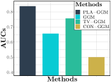
(a) $p=10$

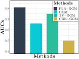
(b) $p=20$

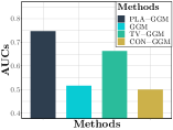
(c) $p=50$

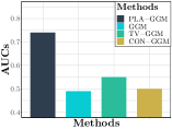
(d) $p=100$

Figure 1: Area under curve (AUC) of considered methods for the structure learning with different numbers of variables.

In Theorem 1, the value of $g^{*}$ does not affect the $\sqrt{n}$-sparsistency of the estimator. In practice, however, if $g^{*}$ is too small, the $\left(\mathbf{D}_{ij}^{\top}\mathbf{W}_{i}\mathbf{D}_{ij}\right)$ tends to be singular, since few samples are observed with $\absolutevalue{g}\leq g^{*}$. Accordingly, the PPL method will be not applicable. Therefore, we need to observe some non-confounded samples to implement the PPL method. The $\sqrt{n}$-sparsistency is not directly related to the selected $\mathds{1}_{\left\{\absolutevalue{g}\geq g^{*}\right\}}$ either. Along the proof of Theorem 1 in the Supplements, we notice that $\mathds{1}_{\left\{\absolutevalue{g}\geq g^{*}\right\}}$ (and thus $g^{*}$) can only affect some auxiliary constants. Since this relationship is neither significant, nor straightforward, we do not discuss it here.

5 Related Methods

After a thorough analysis on the proposed PLA-GGM and PPL method, we now study some related methods that fall into four categories: Gaussian graphical models incorporating confounders, denoted by CON-GGMs; the Gaussian graphical models using linear regression to deal with confounders (Van Dijk et al., 2012; Power et al., 2014) denoted by LR-GGMs; original Gaussian graphical models only using non-confounded samples, denoted by GGMs; and time-varying Gaussian graphical models (Kolar et al., 2010b; Yang et al., 2015b) denoted by TV-GGMs. Theoretically, the proposed PLA-GGM is more generalized and facilitates faster-converging estimators than the existing models.

5.1 CON-GGMs and LR-GGMs

Although not designed for this task, it is possible to apply more standard graphical modeling approaches to deal with some of the effects of observed confounders. For instance, a straightforward alternative to PLA-GGMs is to directly incorporate the confounder as a random variable into the GGM. Specifically, CON-GGMs assume that the confounder $G$ follows a GGM jointly with the random vector $\mathbf{Z}$, which means

$$\left(G,\mathbf{Z}\right)\sim\text{GGM}(\mathbf{\Omega}),$$ (6)

where the joint covariance matrix follows

$$\mathbf{\Sigma}:=\mathbf{\Omega}^{-1}=\begin{bmatrix}\mathbf{\Sigma}_{\mathbf{Z}\mathbf{Z}}&\mathbf{\Sigma}_{\mathbf{Z}G}\\ \mathbf{\Sigma}_{G\mathbf{Z}}&\mathbf{\Sigma}_{GG}\end{bmatrix}.$$

Since the target structure is for $\mathbf{Z}\>|\>G=0$, we can estimate $\mathbf{\Omega}$ by graphical Lasso (Friedman et al., 2008) first, and then derive the inverse conditional covariance matrix for $\mathbf{Z}\>|\>G=0$.

LR-GGM is a model widely used in the neuroscience area (Van Dijk et al., 2012; Power et al., 2014), assuming that the confounders will cause a linear confounding to the observed samples. The model can be formulated as:

$$\mathbf{Z}=\bm{\beta}^{\top}G+\mathbf{Z}^{\prime},$$ (7)

where $\mathbf{Z}^{\prime}$ follows a Gaussian graphical model with parameter $\mathbf{\Omega}$, and $G$ satisfies Assumption 3. Since conditional on $G=0$, $\mathbf{Z}$ is equivalent to $\mathbf{Z}^{\prime}$, the target parameter for the non-confounded structure is just $\mathbf{\Omega}$. LR-GGMs use linear regressions to recover $\bm{\beta}$, and further to regress out confoundings. Finally, LR-GGMs estimate $\mathbf{\Omega}_{0}$ by graphical Lasso.

By deriving the inverse covariance matrices of $\mathbf{Z}$ conditional on $G$ for both CON-GGMs and LR-GGMs, it should be noticed that the inverse conditional covariance matrices are irrelevant to the value of $G$. In other words, the confounder $G$ does not affect the conditional independence structure of $\mathbf{Z}$, which is often an unrealistic restriction. In contrast, PLA-GGM particularly deals with confounding of the structure by $G$. Further following this direction, we can derive the following theorem which describes the the relationship among CON-GGMs, LR-GGMs, and PLA-GGMs.

Theorem 2.

The CON-GGM (6) and the LR-GGM (7) are two special cases of the PLA-GGM by respectively assuming:

• $G$ follows a normal distribution, $\mathbf{R}(g):=0$ and $\mathbf{\Omega}_{0}:=\left[\mathbf{\Sigma}_{\mathbf{Z}\mathbf{Z}}-\mathbf{\Sigma}_{\mathbf{Z}G}\mathbf{\Sigma}_{GG}^{-1}\mathbf{\Sigma}_{G\mathbf{Z}}\right]^{-1}$;

• $\mathbf{R}(g):=0$.

Thus, it is clear that CON-GGMs and LR-GGMs both assume a constant underlying structure irrelevant to $G$, and are parametric special cases of the proposed PLA-GGMs. Also, since the two methods assume $\mathbf{R}(g)=0$ either exactly or asymptotically, they will treat the average of $\mathbf{\Omega}(g)$ as the underlying $\mathbf{\Omega}_{0}$ and derive incorrect structures that are too dense.

5.2 GGMs and TV-GGMs

In PLA-GGMs, it is assumed that some non-confounded samples are observed. Therefore, we can directly apply GGM to the non-confounded samples and estimate the structure. However, by doing this, only the information from the non-confounded data are used. The estimators are obviously not $\sqrt{n}$-sparsistent, considering that most of the $n$ observed samples are confounded and not used by GGM. Thus, the method is less accurate than PLA-GGM.

Another class of relevant methods are time-varying graphical models (TV-GMs) (Song et al., 2009a, b; Kolar et al., 2010b; Kolar & Xing, 2012), used to estimate a different parameter at each time point or observation. Specifically, TV-GGMs assume that $\mathbf{Z}$ follows a varying Gaussian graphical model over $G$. Methods like fused Lasso (Yang et al., 2015b; Zhu & Koyejo, 2018) and the kernel estimation (Kolar et al., 2010b) are applied to estimate the varying structure of $\mathbf{Z}$. One may consider applying such a model, then perhaps averaging the time-varying graph to estimate the non-confounded component. However, since the target of such methods are multiple structures, the estimators can only be guaranteed to be $n^{-2/5}$-consistent. In contrast, PLA-GGMs use all the samples to recover the parameter representing the underlying non-confounded structure, and can achieve $\sqrt{n}$-sparsistency.

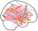
(a) Controls
PLA-GGM

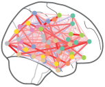
(b) Schizophrenia
PLA-GGM

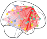
(c) Controls
LR-GGM

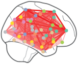
(d) Schizophrenia
LR-GGM

Figure 2: Glass brains for the estimated brain functional connectivity for subjects with schizophrenia and controls using PLA-GGMs and LR-GGMs.

5.3 Graphical Models with Nonparametric Methods

PLA-GMM is not the first approach to incorporate nonparametric methods into graphical models. Prior works like Liu et al. 2009; Kolar et al. 2010a; Voorman et al. 2013; Wang & Kolar 2014; Suggala et al. 2017, and Lu et al. 2015, 2018 have tried to relax the parametric definition of graphical models to realize a more generalized model. However, these methods do not help much to deal with observed confounders, since the structure among the random variables is assumed to be independent of the values of the confounders. Partially linear additive models have also been combined with directed acyclic graphs in (Rothenhäusler et al., 2018), which was developed for causal inference and not the structure analysis.

6 Experiments

To demonstrate the empirical performance of the proposed PLA-GGM and PPL method, we apply them to synthetic data for a structure recovery task in Section 6.1 and a real fMRI dataset for a brain functional connectivity estimation task in Section 6.2.

6.1 Structure Recovery

In this section, we use simulated data to compare PLA-GGM, TV-GGM and CON-GGM discussed in Section 5, with the proposed PLA-GGM for structure recovery. We simulate data from PLA-GGMs following the procedure provided in the Supplement. We consider the case of $p=10,20,50,100$. For all these settings, we fix $n=800$ samples. Then, the four methods are applied to the generated datasets to recover the underlying conditional independence structure. The regularization parameter $\lambda$ is selected by 10-fold cross validation from a series of auto generated $\lambda$’s by glmnet. The bandwidth is determined according to Assumption 1. We use $\mathds{1}_{\left\{\absolutevalue{g}\geq g^{*}\right\}}=1-\exp(-k^{2}g^{2})/2$, where $k$ is selected according to the designated $g^{*}$. We have also studied other forms for $\mathds{1}_{\left\{\absolutevalue{g}\geq g^{*}\right\}}$, which did not significantly affect the performance.

The achieved area under curve (AUC) of the receiver operating characteristic using the selected hyper parameters are reported in Figure 1. Consistent with the analysis in Section 5, the proposed PLA-GGM achieves higher AUCs on structure recovery than the competing methods. Also, as the number of variables increases, the advantage of PLA-GGM gets more significant. The phenomenon results from the $\sqrt{n}$-sparsistency of the $L_{1}$-regularized MaPPLE, which is more accurate and requires less data. It should also be noticed that the AUC achieved by CON-GGM is always around 0.5. The reason is that, following the data simulation procedure, the true $\mathbf{\Omega}(g_{i})$’s are always dense, although $\mathbf{\Omega}_{0}$ is sparse. As suggested by the analysis in Section 5, CON-GGM treats $\mathbf{\Omega}(g)$ as the $\mathbf{\Omega}_{0}$, and thus tends to recover a wrongly dense $\mathbf{\Omega}_{0}$.

6.2 Brain Functional Connectivity Estimation

We apply the PLA-GGM to the 1000 Functional Connectomes Project Cobre dataset (COBRE, 2019), from the Center for Biomedical Research Excellence. The dataset contains 147 subjects with 72 subjects with schizophrenia and 75 healthy controls. For each subject, resting state fMRI time series and the corresponding confounders are recorded. We use the 7 confounders provided in the dataset relate to motion for the analysis, and apply Harvard-Oxford Atlas to select the 48 atlas regions of interest (ROIs). Additional preprocessing details are deferred to the dataset authors (COBRE, 2019). The performance of PLA-GGM is compared to LR-GGM, which is the most widely-used method to deal with motion confounding in the fMRI literature (Van Dijk et al., 2012; Power et al., 2014).

We use $\mathds{1}_{\left\{\absolutevalue{g}\geq g^{*}\right\}}=1-\exp(-100g^{2})/2$ for the following analysis, which is equivalent to $g^{*}=0.578$. If the selected $g^{*}$ is less than the largest possible value, the estimation should still be accurate, since (2) is satisfied. However, a too small $g^{*}$ may induce a singular $\left(\mathbf{D}_{ij}^{\top}\mathbf{W}_{i}\mathbf{D}_{ij}\right)$ and thus the failure of the PPL method. We select the smallest $g^{*}$ where PPL can be successfully implemented, and use the corresponding $\mathds{1}_{\left\{\absolutevalue{g}\geq g^{*}\right\}}$. The results using other $g^{*}$’s and $\mathds{1}_{\left\{\absolutevalue{g}\geq g^{*}\right\}}$’s are reported in the Supplements. Due to Theorem 1, the form of $\mathds{1}_{\left\{\absolutevalue{g}\geq g^{*}\right\}}$ does not affect the sparsistency of the estimator, and thus has a limited effect on the performance.

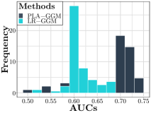
(a) Diagnosis using structures.

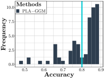
(b) Diagnosis using $\hat{\mathbf{\Omega}}_{0}$.

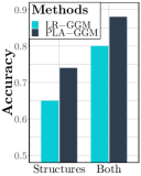
Figure 3: AUCs for the diagnosis of schizophrenia using only the structures or $\hat{\mathbf{\Omega}}_{0}$ with different regularization parameters.

   Figure 4: AUCs for the diagnosis of schizophrenia with the regularization parameters selected by AIC.

General Analysis

We first generally analyze the brain functional connectivity by the PLA-GGM. Specifically, following the common practice in this area (Belilovsky et al., 2016), we assume that all the fMRIs from the subjects with schizophrenia follow a single PLA-GGM with the same brain functional connectivity, and thus combine the preprocessed fMRIs from the subjects into one dataset. Then, the PPL method is applied to the combined dataset to estimate an $\mathbf{\Omega}_{0}$, which corresponds to the brain functional connectivity for all the subjects with schizophrenia. The same procedure is also implemented on the control subjects’ fMRI datsets.

For a comparison, we also apply the LR-GGM discussed in Section 5 by the aforementioned procedure. The estimated brain functional connectivity for subjects and the controls with the two methods are reported in Figure 2. The ROIs are denoted by nodes with different colors. Edges among nodes denote the estimated functional connectivity. Red edges denote the positive connections, while the blues ones denote negative connections. The darker the color, the stronger the connection. We only provide the figure from one angle here. The figures from other angles are provided in the Supplements.

Comparing the glass brain figure for controls with the one for subjects estimated by PLA-GGM, we find Occipital Pole and Central Opercular Cortex are the two areas differ the most. Interestingly, these two areas have been implicated in the literature as highly associated with schizophrenia (Sheffield et al., 2015). Also, by comparing the results of PLA-GGMs with those of LR-GGMs, the results of LR-GGMs are much denser and covered with lots of positive connections. This phenomenon is consistent with our analysis in Section 5: LR-GGMs will treat the average of $\mathbf{\Omega}(g)$’s as the estimator to $\mathbf{\Omega}_{0}$ and derive incorrect over-dense estimates. This strongly suggests that the dense structure here is a result of the confounders which are not successfully accounted for by the regression.

Schizophrenia Diagnosis

Ideally, to demonstrate the accuracy of the proposed method for structure recovery, we should compare the estimated brain functional connectivity to the underlying ground truth, which, however, is not available in practice. Therefore, we consider a surrogate evaluation by using the estimated functional connectivity for schizophrenia diagnosis. Intuitively, if the recovered connectivity is more accurate due to effectively omitting the confounding, we should be able to improve schizophrenia diagnosis using the estimated connectivity as features. We apply PLA-GGMs and LR-GGMs to each subject respectively, and calculate $\hat{\mathbf{\Omega}}_{0}$’s for every subject. Then, we use $\hat{\mathbf{\Omega}}_{0}$’s as the input for classification methods to classify the subjects. For this two-class classification task, we use an $L_{1}$-regularized logistic regression as this is a common approach in the literature (Patel et al., 2016).

We consider using only the structure (signs without values) of $\hat{\mathbf{\Omega}}_{0}$’s as the input for the classification. Although the classification is of course more challenging, we can more clearly see how helpful the structure itself is for the diagnosis. The AUCs for the diagnosis are reported in Figure 3(a). For a thorough comparison, we use the regularization parameters suggested by the R package glmnet for the penalized logistic regression and report all the AUCs. Clearly, PLA-GGMs resut in more accurate prediction. Therefore, the brain connectivity estimators derived by PLA-GGMs are more informative for schizophrenia diagnosis and more accurate than those of LR-GGMs.

We next include the values into the input, and evaluate the accuracy for schizophrenia diagnosis. Again, we report all the results using different regularization parameters in Figure 3(b). The green line indicates the best performance of using LR-GGM and $L_{1}$-regularized logistic regression achieved in (Patel et al., 2016). Since we are using exactly the same dataset, we directly use their results for the LR-GGM combined with penalized logistic regression for a fair comparison. As a result, for most of the regularization parameters, PLA-GGMs derive more accurate diagnosis than LR-GGMs. Experiments using different $\mathds{1}_{\left\{\absolutevalue{g}\geq g^{*}\right\}}$ are included in the Supplements. The results are similar. Therefore, we conclude that PLA-GGMs more accurately address confounding and derive more accurate estimators of brain functional connectivity.

We note, however, that some specialized alternative classifiers have been developed in the brain connectivity literature (Patel et al., 2016; Arroyo-Relión et al., 2017; Andersen et al., 2018), and expect that our approach will improve performance for those classifiers as well. We leave such further analysis to future work.

7 Conclusions and Future Works

We propose PLA-GGMS, to study the relationships among random variables with observed confounders. PLA-GGMs are especially generalized and facilitate $\sqrt{n}$-sparsisent estimators. The utility of PLA-GGMs is demonstrated using a real-world fMRI dataset for the brain connectivity estimation. While we have been taking GGMs as an example, the results can be generalized to other undirected graphical models, especially the univariate exponential family distributions (UEFDs) (Yang et al., 2015a). We leave the details to future work.

Supplements

Appendix A Proof of Theorem 1

Following the definition, we can derive the PL for the PLA-GGM as:

$$\begin{split}\ell_{PL}\left(\left\{\mathbf{z}_{i},g_{i}\right\}_{i\in[n]};\mathbf{R}(\cdot),\mathbf{\Omega}_{0}\right)\propto&\sum_{i=1}^{n}\sum_{j=1}^{p}\left\{z_{ij}\left(\Omega_{ijj}+\sum_{j^{\prime}\neq j}\Omega_{ijj^{\prime}}z_{ij}z_{ij^{\prime}}\right)-\frac{1}{2}z_{ij}^{2}\right.\\ &-\left.\frac{1}{2}\left(\Omega_{ijj}+\sum_{j^{\prime}\neq j}\Omega_{ijj^{\prime}}z_{ij}z_{ij^{\prime}}\right)^{2}\right\}.\end{split}$$

Then Lemma 1 can be proved by the definition of $\mathbf{z}_{i,-j}$.

Appendix B Proof of Lemma 2

According to the analysis in Section 3.1, we treat the PL as $p$ partially-linear additive linear regressions. Then, for each regression, we can derive $\hat{M}_{ij}$ as the estimation to the smooth part following the rationale in (Fan et al., 2005). Combining the results for every regression, we can derive Lemma 2.

Appendix C Proof of Theorem 1

In this Section, we prove the $\sqrt{n}$-sparsistency of the $L_{1}$-regularized MPPLE by following the widely-used primal-dual witness proof technique (Wainwright, 2009; Ravikumar et al., 2010; Yang & Ravikumar, 2011; Yang et al., 2015a). PDW is characterized by the following Lemma 3:

Lemma 3.

Let $\hat{\mathbf{\Omega}}_{0}$ be an optimal solution to (5), and $\hat{\mathbf{Z}}$ be the corresponding dual solution. If $\hat{\mathbf{Z}}$ satisfies $\norm{\hat{\mathbf{Z}}_{N}}_{\infty}<1$, then any given optimal solution to (5) $\tilde{\mathbf{\Omega}}_{0}$ satisfies $\tilde{\mathbf{\Omega}}_{0I}=\bm{0}$. Moreover, if $\mathbf{H}_{SS}$ is positive definite, then the solution to (5) is unique.

Proof.

Specifically, following the same rationale as Lemma 1 in Wainwright 2009, Lemma 1 in Ravikumar et al. 2010, and Lemma 2 in Yang & Ravikumar 2011, we can derive Lemma 3 characterizing the optimal solution of (5). ∎

Bound $\norm{\gradient F(\mathbf{\Omega}_{0}^{*})}_{\infty}$

Before we use the PDW, we first provide a Lemma bounding $\norm{\gradient F(\mathbf{\Omega}_{0}^{*})}_{\infty}$, which has been shown to be vital for PDW (Wainwright, 2009; Ravikumar et al., 2010; Yang & Ravikumar, 2011; Yang et al., 2015a).

Lemma 4.

Let $r:=4C_{5}\lambda$. For any $\epsilon_{d}>0$, with probability of at least $1-\epsilon_{d}$, there exists $C_{4}>0$ and $N_{d}>0$ satisfying the following two inequalities:

$$\norm{\gradient F(\mathbf{\Omega}_{0}^{*})}_{\infty}\leq C_{4}\sqrt{\frac{\log p}{n}},$$ (8)

$$\norm{\tilde{\bm{\Theta}}_{S}-\bm{\Theta}^{*}_{S}}_{\infty}\leq r,$$ (9)

for $n>N_{d}$.

Proof.

We prove (8) and (9) in turn.

Proof of (8)

To begin with, we prove (8). We define

$$\lambda_{ij}^{*}=\left(\bm{1}_{i}-\mathbf{S}_{ij}\right)^{\top}\mathbf{x}_{j}\mathbf{\Omega}^{*}_{0\cdot j}.$$

We use the $F$ to denote the PPL defined in Definition 1. Then, the derivative of $F(\mathbf{\Omega}^{*}_{0\cdot j})$ is:

$$\begin{split}\frac{\partial F(\mathbf{\Omega}^{*}_{0})}{\partial\Omega^{*}_{0j^{\prime}j}}=&\frac{\sum_{i=1}^{n}\left\{-\left(\bm{1}_{i}-\mathbf{S}_{ij}\right)^{\top}\mathbf{y}_{j}\left[\left(\bm{1}_{i}-\mathbf{S}_{ij}\right)^{\top}\mathbf{x}_{j}\right]_{j^{\prime}}+\lambda_{ij}^{*}\left[\left(\bm{1}_{i}-\mathbf{S}_{ij}\right)^{\top}\mathbf{x}_{j}\right]_{j^{\prime}}\right\}}{n}\\ &+\frac{\sum_{i=1}^{n}\left\{-\left(\bm{1}_{i}-\mathbf{S}_{ij^{\prime}}\right)^{\top}\mathbf{y}_{j^{\prime}}\left[\left(\bm{1}_{i}-\mathbf{S}_{ij^{\prime}}\right)^{\top}\mathbf{x}_{j^{\prime}}\right]_{j}+\lambda_{ij^{\prime}}^{*}\left[\left(\bm{1}_{i}-\mathbf{S}_{ij}\right)^{\top}\mathbf{x}_{j^{\prime}}\right]_{j}\right\}}{n},\end{split}$$ (10)

where $[\cdot]_{j}$ denotes the $j^{\text{th}}$ component of the vector. For the ease of presentation, we define

$$\mathbf{y}_{j}^{\prime}=\begin{bmatrix}\left(\bm{1}_{1}-\mathbf{S}_{1j}\right)^{\top}\mathbf{y}_{j}\\ \vdots\\ \left(\bm{1}_{n}-\mathbf{S}_{nj}\right)^{\top}\mathbf{y}_{j}\end{bmatrix}\text{ and }\mathbf{x}_{j}^{\prime}=\begin{bmatrix}\left(\bm{1}_{1}-\mathbf{S}_{1j}\right)^{\top}\mathbf{x}_{j}\\ \vdots\\ \left(\bm{1}_{n}-\mathbf{S}_{nj}\right)^{\top}\mathbf{x}_{j}\end{bmatrix}.$$

Then, we consider

$$\frac{{\mathbf{x}_{j}^{\prime}}^{\top}\mathbf{x}_{j}^{\prime}\mathbf{\Omega}_{0\cdot j}^{*}-{\mathbf{x}_{j}^{\prime}}^{\top}\mathbf{y}_{j}^{\prime}}{n},$$ (11)

whose $j^{\prime\text{th}}$ component is just the target value

$$\frac{\sum_{i=1}^{n}\left\{-\left(\bm{1}_{i}-\mathbf{S}_{ij}\right)^{\top}\mathbf{y}_{j}\left[\left(\bm{1}_{i}-\mathbf{S}_{ij}\right)^{\top}\mathbf{x}_{j}\right]_{j^{\prime}}+\lambda_{ij}^{*}\left[\left(\bm{1}_{i}-\mathbf{S}_{ij}\right)^{\top}\mathbf{x}_{j}\right]_{j^{\prime}}\right\}}{n}.$$

Therefore, we focus on bounding (11). Then,

$$\begin{split}\frac{{\mathbf{x}_{j}^{\prime}}^{\top}\mathbf{x}_{j}^{\prime}\mathbf{\Omega}_{0\cdot j}^{*}-{\mathbf{x}_{j}^{\prime}}^{\top}\mathbf{y}_{j}^{\prime}}{n}=&\frac{{\mathbf{x}_{j}^{\prime}}^{\top}\mathbf{x}_{j}^{\prime}\left[\mathbf{\Omega}_{0\cdot j}^{*}-\left({\mathbf{x}_{j}^{\prime}}^{\top}\mathbf{x}_{j}^{\prime}\right)^{-1}{\mathbf{x}_{j}^{\prime}}^{\top}\mathbf{y}_{j}^{\prime}\right]}{n}\\ =&\frac{{\mathbf{x}_{j}^{\prime}}^{\top}\left(\mathbf{I}-\mathbf{S}_{j}\right)(\mathbf{M}_{j}+\bm{\epsilon}_{j})}{n}\end{split},$$

where the second equality is due to Lemma 5.

We fist study $\frac{{\mathbf{X}_{j}^{\prime}}^{\top}\left(\mathbf{I}-\mathbf{S}_{j}\right)\mathbf{M}_{j}}{n}$: according ot Lemma 8, for any $\epsilon_{a}>0$, there exists $\delta_{a}>0$ and $N_{a}>0$ satisfying

$$\text{P}\left\{\norm{\frac{{\mathbf{x}_{j}^{\prime}}^{\top}\left(\mathbf{I}-\mathbf{S}_{j}\right)\mathbf{M}_{j}}{n}}_{\infty}>\delta_{a}\left[\frac{\log(\frac{1}{h})}{nh}+h^{4}+2h^{2}\sqrt{\frac{\log(\frac{1}{h})}{nh}}\right]\right\}<\epsilon_{a},$$

with $n>N_{a}$.

According to Assumption 1

$$\text{P}\left\{\norm{\frac{{\mathbf{x}_{j}^{\prime}}^{\top}\left(\mathbf{I}-\mathbf{S}_{j}\right)\mathbf{M}_{j}}{n}}_{\infty}>\delta_{a}C_{1}\sqrt{\frac{\log p}{n}}\right\}<\epsilon_{a}.$$ (12)

Now, we study $\frac{{\mathbf{x}_{j}^{\prime}}^{\top}\left(\mathbf{I}-\mathbf{S}_{j}\right)\bm{\epsilon}_{j}}{n}$. According to Lemma 9, we have

$$\frac{{\mathbf{x}_{j}^{\prime}}^{\top}\left(\mathbf{I}-\mathbf{S}_{j}\right)\bm{\epsilon}_{j}}{n}=\sum_{i=1}^{n}\left\{\mathbf{x}_{ij}-\mathbb{E}^{\top}\left[\mathds{1}_{g_{i^{\prime}}>g^{*}}\mathbf{Z}_{i,-j}\mathbf{Z}_{i,-j}^{\top}\>|\>g_{i}\right]\mathbb{E}^{-1}\left[\mathds{1}^{2}_{g_{i^{\prime}}>g^{*}}\mathbf{Z}_{i,-j}\mathbf{Z}_{i,-j}^{\top}\>|\>g_{i}\right]\tilde{\mathbf{x}}_{ij}\right\}$$

$$\epsilon_{ij}(1+o_{p}(1))/n,$$

uniformly for $j$. Note that $\frac{{\mathbf{x}_{j}^{\prime}}^{\top}\left(\mathbf{I}-\mathbf{S}_{j}\right)\bm{\epsilon}_{j}}{n}$is a $p\times 1$ vector. Therefore, for the ${j^{\prime}}^{\text{th}}$ component, we have

$$\begin{split}&\absolutevalue{\left[\frac{{\mathbf{x}_{j}^{\prime}}^{\top}\left(\mathbf{I}-\mathbf{S}_{j}\right)\bm{\epsilon}_{j}}{n}\right]_{j^{\prime}}}\\ \leq&\absolutevalue{\sum_{i:g^{i}\leq g^{*}}\left(1-\mathds{1}^{2}_{g^{i}>g^{*}}\right)z_{ij^{\prime}}\epsilon_{ij}}\left(1+\absolutevalue{o_{p}(1)}\right)/n\\ =&\frac{1}{2n}\absolutevalue{\sum_{i=1}\left(1-\mathds{1}^{2}_{g_{i}>g^{*}}\right)\left[\left(\frac{z_{ij^{\prime}}+\epsilon_{ij}}{\sqrt{2}}\right)^{2}-1-\left(\frac{z_{ij^{\prime}}-\epsilon_{ij}}{\sqrt{2}}\right)^{2}+1\right]}(1+\absolutevalue{o_{p}(1)})\end{split}.$$ (13)

It can be shown that $\left(\frac{z_{ij^{\prime}}+\epsilon_{ij}}{\sqrt{2}}\right)^{2}$ and $\left(\frac{z_{ij^{\prime}}-\epsilon_{ij}}{\sqrt{2}}\right)^{2}$ are independent and follow chi-squared distribution with degree equal to $1$.

By Lemma 1 in (Laurent & Massart, 2000), the linear combinition of chi-squared random variables satisfies:

$$\text{P}\left\{\sum_{i=1}\left(1-\mathds{1}^{2}_{g_{i}>g^{*}}\right)\left[\left(\frac{z_{ij^{\prime}}+\epsilon_{ij}}{\sqrt{2}}\right)^{2}-1\right]\geq 2\sqrt{nx}+2\epsilon_{c}\right\}\leq\exp(-\epsilon_{c}),$$

$$\text{P}\left\{\sum_{i=1}\left(1-\mathds{1}^{2}_{g_{i}>g^{*}}\right)\left[\left(\frac{z_{ij^{\prime}}+\epsilon_{ij}}{\sqrt{2}}\right)^{2}-1\right]\leq-2\sqrt{nx}\right\}\leq\exp(-\epsilon_{c}),$$

$$\text{P}\left\{-\sum_{i=1}\left(1-\mathds{1}^{2}_{g_{i}>g^{*}}\right)\left[\left(\frac{z_{ij^{\prime}}-\epsilon_{ij}}{\sqrt{2}}\right)^{2}-1\right]\leq-2\sqrt{nx}-2\epsilon_{c}\right\}\leq\exp(-\epsilon_{c}),$$

and

$$\text{P}\left\{-\sum_{i=1}\left(1-\mathds{1}^{2}_{g_{i}>g^{*}}\right)\left[\left(\frac{z_{ij^{\prime}}-\epsilon_{ij}}{\sqrt{2}}\right)^{2}-1\right]\geq 2\sqrt{nx}\right\}\leq\exp(-\epsilon_{c}),$$

for any $\epsilon_{c}>0$. Combing the previous four probabilistic bounds, we can derive

$$\begin{split}\text{P}\left\{\sum_{i=1}\left(1-\mathds{1}^{2}_{g_{i}>g^{*}}\right)\left[\left(\frac{z_{ij^{\prime}}+\epsilon_{ij}}{\sqrt{2}}\right)^{2}-1\right]\right.&\\ -\sum_{i=1}\left(1-\mathds{1}^{2}_{g_{i}>g^{*}}\right)&\left.\left[\left(\frac{z_{ij^{\prime}}-\epsilon_{ij}}{\sqrt{2}}\right)^{2}-1\right]\geq 4\sqrt{n\epsilon}+2\epsilon_{c}\right\}\leq\exp(-2\epsilon_{c})\end{split}$$ (14)

and

$$\begin{split}\text{P}\left\{\sum_{i=1}\left(1-\mathds{1}^{2}_{g_{i}>g^{*}}\right)\left[\left(\frac{z_{ij^{\prime}}+\epsilon_{ij}}{\sqrt{2}}\right)^{2}-1\right]\right.&\\ -\sum_{i=1}\left(1-\mathds{1}^{2}_{g_{i}>g^{*}}\right)&\left.\left[\left(\frac{z_{ij^{\prime}}-\epsilon_{ij}}{\sqrt{2}}\right)^{2}-1\right]\leq-4\sqrt{n\epsilon}-2\epsilon_{c}\right\}\leq\exp(-2\epsilon_{c})\end{split}.$$ (15)

Taking (14) and (15) into (13), we can derive

$$\begin{split}\text{P}\left\{\absolutevalue{\left[\frac{{\mathbf{X}_{j}^{\prime}}^{\top}\left(\mathbf{I}-\mathbf{S}_{j}\right)\bm{\epsilon}_{j}}{n}\right]_{j^{\prime}}}\geq\left(2\sqrt{\frac{\epsilon_{c}}{n}}+\frac{\epsilon_{c}}{n}\right)(1+\absolutevalue{o_{p}(1)})\right\}\leq 2\exp(-2\epsilon_{c})\end{split}.$$ (16)

Then, by the definition of $o_{p}(1)$, for any $\epsilon_{b}>0$, there exists $N_{b}$ so that for $n>N_{b}$:

$$\text{P}\left\{\absolutevalue{o_{p}(1)}\geq 1\right\}\leq\epsilon_{b}.$$ (17)

Combining (16) and (17), we derive

$$\begin{split}\text{P}\left\{\norm{\frac{{\mathbf{X}_{j}^{\prime}}^{\top}\left(\mathbf{I}-\mathbf{S}_{j}\right)\mathbf{M}_{j}}{n}}_{\infty}\geq\left(4\sqrt{\frac{\epsilon_{c}}{n}}+2\frac{\epsilon_{c}}{n}\right)\right\}\leq 2p\exp(-2\epsilon_{c})+\epsilon_{b}\end{split},$$ (18)

by a union bound. Eventually, according to (12) and (18), and by setting $\epsilon_{c}=2\log p$ we prove:

$$\norm{\frac{{\mathbf{x}_{j}^{\prime}}^{\top}\mathbf{x}_{j}^{\prime}\mathbf{\Omega}_{0\cdot j}^{*}-{\mathbf{x}_{j}^{\prime}}^{\top}\mathbf{y}_{j}^{\prime}}{n}}_{\infty}\leq(6+\delta_{a}C_{1})\sqrt{\frac{2\log p}{n}},$$

with probability larger than $1-\epsilon_{b}-\epsilon_{a}-2p^{-1}$. Thus, for any $\epsilon_{d}>0$, there exists $C_{4}>0$ and $N_{d}>0$

$$\norm{\gradient F(\bm{\Theta}^{*})}_{\infty}\leq C_{4}\sqrt{\frac{\log p}{n}},$$

with probability larger than $1-\epsilon_{d}$, for $n>N_{d}$.

Proof of (9)

To prove (9), we use the fixed point method by defining a map $G(\bm{\Delta}_{S}):=-\mathbf{H}_{SS}^{-1}\left[\gradient_{S}F(\mathbf{\Omega}^{*}_{0S}+\bm{\Delta}_{S})+\lambda\hat{\mathbf{Z}}_{S}\right]+\bm{\Delta}_{S}$. If $\norm{\bm{\Delta}}_{\infty}\leq r$, by Taylor expansion of $\gradient_{S}F(\mathbf{\Omega}_{0}^{*}+\bm{\Delta})$ centered at $\gradient_{S}F(\mathbf{\Omega}_{0}^{*})$,

$$\left\lVert G(\bm{\Delta}_{S})\right\rVert_{\infty}= \left\lVert-\mathbf{H}_{SS}^{-1}\left[\gradient_{S}F(\mathbf{\Omega}^{*}_{0S})+\mathbf{H}_{SS}\bm{\Delta}_{S}+\bm{R}_{S}(\bm{\Delta})+\lambda\hat{\mathbf{Z}}_{S}\right]+\bm{\Delta}_{S}\right\rVert_{\infty}$$

$$= \left\lVert-\mathbf{H}_{SS}^{-1}\left(\gradient_{S}F(\mathbf{\Omega}^{*}_{0S})+\bm{R}_{S}(\bm{\Delta})+\lambda\hat{\mathbf{Z}}_{S}\right)\right\rVert_{\infty}$$

$$\leq \left\lVert\mathbf{H}_{SS}^{-1}\right\rVert_{\infty}\left(\norm{\gradient_{S}F(\mathbf{\Omega}^{*}_{0S})}_{\infty}+\norm{R_{S}(\bm{\Delta})}_{\infty}+\lambda\norm{\hat{\mathbf{Z}}_{S}}_{\infty}\right)$$

$$\leq C_{2}(\lambda+C_{3}r^{2}+\lambda)=C_{2}C_{3}r^{2}+2C_{2}\lambda,$$

where the inequality is due to Assumption 4 and Assumption 5, and $\norm{\gradient_{S}F(\bm{\Theta}^{*})}_{\infty}\leq\lambda$ with a high probability, according to (8). Then, based on the definition of $r$, we can derive the upper bound of $\left\lVert G(\bm{\Delta}_{S})\right\rVert_{\infty}$ as $\left\lVert G(\bm{\Delta}_{S})\right\rVert_{\infty}\leq r/2+r/2=r$.

Therefore, according to the fixed point theorem (Ortega & Rheinboldt, 2000; Yang & Ravikumar, 2011), there exists $\bm{\Delta}_{S}$ satisfying $G(\bm{\Delta}_{S})=\bm{\Delta}_{S}$, which indicates $\gradient_{S}F(\mathbf{\Omega}_{0}^{*}+\bm{\Delta})+\lambda\hat{\mathbf{Z}}_{S}=\bm{0}$. The optimal solution to (20) is unique, and thus $\tilde{\bm{\Delta}}_{S}=\bm{\Delta}_{S}$. Therefore, $\norm{\tilde{\bm{\Delta}}_{S}}_{\infty}\leq r$ , with probability larger than $1-\epsilon$. ∎

PDW

By Lemma 3, we can prove the sparsistency by building an optimal solution to (5) satisfying the strict dual feasibility (SDF) defined as $\norm{\hat{\mathbf{Z}}_{N}}_{\infty}<1$, which is summarized. Therefore, we now build a solution by solving a restricted problem.

Solve a Restricted Problem

First of all, we derive the KKT condition of (5):

$$\gradient F(\hat{\mathbf{\Omega}}_{0})+\lambda\hat{\mathbf{Z}}=\bm{0}.$$ (19)

To construct an optimal primal-dual pair solution, we define $\tilde{\mathbf{\Omega}}_{0}$ as an optimal solution to the restricted problem:

$$\begin{split}\tilde{\mathbf{\Omega}}_{0}:=\min_{\mathbf{\Omega}_{0}}F(\mathbf{\Omega}_{0})+\lambda\norm{\mathbf{\Omega}_{0}}_{1},\end{split}$$ (20)

with ${\mathbf{\Omega}_{0}}_{N}=\mathbf{0}$. $\tilde{\mathbf{\Omega}}_{0}$ is unique due to Lemma 3. Then, we define the subgradient corresponding to $\tilde{\mathbf{\Omega}}_{0}$ as $\tilde{\mathbf{Z}}$. Therefore, $(\tilde{\mathbf{\Omega}}_{0},\tilde{\mathbf{Z}})$ is a pair of optimal solutions to the restricted problem (20). $\tilde{\mathbf{Z}}_{S}$ is determined according to the values of $\tilde{\mathbf{\Omega}}_{0S}$ via the KKT conditions of (20). Thus we have

$$\gradient_{S}F(\tilde{\bm{\Theta}})+\lambda\tilde{\mathbf{Z}}_{S}=\bm{0},$$ (21)

where $\gradient_{S}$ represents the gradient components with respect to $S$. Letting $\hat{\mathbf{\Omega}}_{0}=\tilde{\mathbf{\Omega}}_{0}$, we determine $\tilde{\mathbf{Z}}_{N}$ according to (19). It now remains to show that $\tilde{\mathbf{Z}}_{N}$ satisfies SDF.

SDF

Now, we demonstrate that $\tilde{\bm{\Theta}}$ and $\tilde{\mathbf{Z}}$ satisfy SDF. We define $\tilde{\bm{\Delta}}:=\tilde{\bm{\Theta}}-\bm{\Theta}^{*}$. By (21), and by the Taylor expansion of $\gradient_{S}F(\tilde{\mathbf{\Omega}}_{0})$, we have that

$$\mathbf{H}_{SS}\tilde{\bm{\Delta}}_{S}+\gradient_{S}F(\mathbf{\Omega}^{*}_{0})+\bm{R}_{S}(\tilde{\bm{\Delta}})+\lambda\tilde{\mathbf{Z}}_{S}=\bm{0},$$

which means

$$\tilde{\bm{\Delta}}_{S}=\mathbf{H}_{SS}^{-1}\left[-\gradient_{S}F(\mathbf{\Omega}_{0}^{*})-\bm{R}_{S}(\bm{\tilde{\Delta}})-\lambda\tilde{\mathbf{Z}}_{S}\right],$$ (22)

where $\mathbf{H}_{SS}$ is positive definite and hence invertible.

By the definition of $\tilde{\mathbf{\Omega}}_{0}$ and $\tilde{\mathbf{Z}}$,

$$\gradient F(\tilde{\mathbf{\Omega}}_{0})+\lambda\tilde{\mathbf{Z}}=\mathbf{0}\Rightarrow\gradient F(\mathbf{\Omega}_{0}^{*})+\mathbf{H}\tilde{\bm{\Delta}}+\bm{R}(\tilde{\mathbf{\Omega}}_{0})+\lambda\tilde{\mathbf{Z}}=\bm{0}\Rightarrow\gradient_{N}F(\tilde{\bm{\Theta}})+\mathbf{H}_{NS}\tilde{\bm{\Delta}}_{S}+\bm{R}_{N}(\tilde{\bm{\Delta}})+\lambda\tilde{\mathbf{Z}}_{N}=\bm{0}.$$ (23)

Due to (22),

$$\begin{split}\lambda\norm{\tilde{\mathbf{Z}}_{N}}_{\infty}=&\norm{-\mathbf{H}_{NS}\tilde{\bm{\Delta}}_{S}-\gradient_{N}F(\mathbf{\Omega}_{0}^{*})-\bm{R}_{N}(\tilde{\bm{\Delta}})}_{\infty}\\ \leq&\left\lVert\mathbf{H}_{NS}\mathbf{H}_{SS}^{-1}\left[-\gradient_{S}F(\mathbf{\Omega}_{0}^{*})-\bm{R}_{S}(\tilde{\bm{\Delta}})-\lambda\tilde{\mathbf{Z}}_{S}\right]\right\rVert_{\infty}+\norm{\gradient_{N}F(\mathbf{\Omega}_{0}^{*})+\bm{R}_{N}(\tilde{\bm{\Delta}})}_{\infty}\\ \leq&\left\lVert\mathbf{H}_{NS}\mathbf{H}_{SS}^{-1}\right\rVert_{\infty}\left\lVert\gradient_{S}F(\mathbf{\Omega}_{0}^{*})+\bm{R}_{S}(\tilde{\bm{\Delta}})\right\rVert_{\infty}+\left\lVert\mathbf{H}_{NS}\mathbf{H}_{SS}^{-1}\right\rVert_{\infty}\left\lVert\lambda\tilde{\mathbf{Z}}_{S}\right\rVert_{\infty}+\norm{\gradient_{N}F(\mathbf{\Omega}_{0}^{*})+\bm{R}_{N}(\tilde{\bm{\Delta}})}_{\infty}\end{split}.$$

Further, we use the Assumption 4,

$$\lambda\norm{\tilde{\mathbf{Z}}_{N}}_{\infty}\leq (1-\alpha)\left(\norm{\gradient_{S}F(\mathbf{\Omega}_{0}^{*})}_{\infty}+\norm{\bm{R}_{S}(\tilde{\bm{\Delta}})}_{\infty}\right)+(1-\alpha)\lambda+\left(\norm{\gradient_{N}F(\mathbf{\Omega}_{0}^{*})}_{\infty}+\norm{\bm{R}_{N}(\tilde{\bm{\Delta}})}_{\infty}\right)$$

$$\leq (2-\alpha)\left(\norm{\gradient F(\mathbf{\Omega}_{0}^{*})}_{\infty}+\norm{\bm{R}(\tilde{\bm{\Delta}})}_{\infty}\right)+(1-\alpha)\lambda,$$ (24)

where we have used in the first inequality, and the third inequality is due to Assumption 4.

Now, we study $\norm{\gradient F(\mathbf{\Omega}_{0}^{*})}_{\infty}$.By Lemma 4 and the assumption on $\lambda$ in Theorem 1, $\norm{\gradient F(\bm{\Theta}^{*})}_{\infty}\leq\frac{\alpha C_{4}}{4}\sqrt{\frac{\log p}{n}}\leq\frac{\alpha\lambda}{4}$, with probability larger than $1-\epsilon_{d}$.

It remains to control $\norm{\bm{R}(\tilde{\bm{\Delta}})}_{\infty}$. According to Assumption 5 and Lemma 4,

$$\norm{\bm{R}(\tilde{\bm{\Delta}})}_{\infty}\leq C_{3}\norm{\bm{\Delta}}_{\infty}^{2}\leq C_{3}r^{2}\leq C_{3}(4C_{2}\lambda)^{2}=\lambda\frac{64C_{2}^{2}C_{3}}{\alpha}\frac{\alpha\lambda}{4}\leq\left(C_{5}\sqrt{\frac{\log p}{n}}\right)\frac{64C_{2}^{2}C_{3}}{\alpha}\frac{\alpha\lambda}{4},$$ (25)

where in the last inequality we have used the assumption $\lambda\leq C_{5}\sqrt{\frac{\log p}{n}}$ in Theorem 1. Therefore, when we choose $n\geq\left(64C_{5}C_{2}^{2}C_{3}/\alpha\right)^{2}\log p$ in Theorem 1, from (25), we can conclude that $\norm{\bm{R}(\tilde{\bm{\Delta}})}_{\infty}\leq\frac{\alpha\lambda}{4}$. As a result, $\lambda\norm{\hat{\mathbf{Z}}_{N}}_{\infty}$ can be bounded by $\lambda\norm{\tilde{\mathbf{Z}}_{N}}_{\infty}<\alpha\lambda/2+\alpha\lambda/2+(1-\alpha)\lambda=\lambda$. Combined with Lemma 3, we demonstrate that any optimal solution of (5) satisfies $\tilde{\bm{\Theta}}_{N}=\bm{0}$. Furthermore, (9) controls the difference between the optimal solution of (5) and the real parameter by $\norm{\tilde{\bm{\Delta}}_{S}}_{\infty}\leq r$, by the fact that $r\leq\norm{\bm{\Theta}^{*}_{S}}_{\infty}$ in Theorem 1, $\hat{\bm{\Theta}}_{S}$ shares the same sign with $\bm{\Theta}^{*}_{S}$.

Auxiliary Lemmas

In this section, we provide and prove the used auxiliary lemmas.

Lemma 5.

For the graphical model defined in Section 2 parameterized by $\mathbf{\Omega}_{0}^{*}$, the conditional distribution of $Z_{ij}$ follows

$$\left(Z_{ij}\>|\>G_{i}=g_{i}\right)\sim\mathbf{Z}_{i,-j}^{\top}\mathbf{\Omega}_{0\cdot j}+M_{ij}+\epsilon_{ij},$$

where

$$\left[\mathbf{Z}_{i,-j}\right]_{j^{\prime}}=\begin{cases}Z_{ij^{\prime}}&j^{\prime}\neq j\\ 1&j^{\prime}=j\end{cases}.$$

$\epsilon_{ij}$’s follow the standard normal distribution, and $\epsilon_{ij}$ is independent with $\epsilon_{i^{\prime}j}$ for $j\neq j^{\prime}\in[p]$.

Proof.

According to Lemma 1, the node-wise conditional distribution of a PLA-GGM follows a Gaussian distribution. Then, Lemma 5 can be proved. ∎

Lemma 6.

For a kernel regression on $\left\{x_{i},y_{i}\right\}_{i=1}^{n}$ as the IID samples of $(X,Y)$. Assume that $\mathbb{E}\absolutevalue{Y}^{s}<\infty$ and $\sup_{X}\in\absolutevalue{Y}^{s}f(X,Y)dY\leq\infty$. Given that $n^{2\epsilon-1}h\to\infty$ for $\epsilon<1-s^{-1}$, we have

$$\sum_{x}\absolutevalue{\frac{1}{n}\sum_{i=1}^{n}\left[K_{h}(x_{i}-x)-\mathbb{E}\left\{K_{h}(x_{i}-x)y_{i}\right\}\right]}=O_{p}\left(\left\{\frac{\log(1/h)}{nh}\right\}^{1/2}\right).$$

Proof.

Lemma 6 follows (Mack & Silverman, 1982). ∎

Lemma 7.

Suppose $\mathbf{Y}=\left\{Y_{1},Y_{2}\cdots,Y_{n}\right\}$ follows a multivariate Gaussian distribution, then $\max\absolutevalue{Y_{i}}$ follows a sub-Gaussian distribution with variance $\max\text{var}(Y_{i})$. Further, for any $t>0$, the tail probability can be controlled via

$$\text{P}\left\{\max\absolutevalue{\epsilon_{ij}}\geq t\right\}\leq\exp\left(\frac{-t^{2}}{2}\right).$$

Lemma 8.

For any $\epsilon>0$, there exists $\delta>0$ and $N>0$, so that when $n>N$, we have

$$\text{P}\left\{\norm{\frac{\mathbf{X}_{j}^{\prime}(\mathbf{I}-\mathbf{S}_{j})\mathbf{M}_{j}}{n}}_{\infty}\geq\delta c^{2}_{n}\right\}\leq\epsilon,$$

uniformly for $j\in[p]$.

Proof.

To start with, we review the definition of $\mathbf{S}_{ij}$

$$\mathbf{S}_{ij}=\begin{bmatrix}\mathds{1}_{g_{i^{\prime}}>g^{*}}\mathbf{z}_{i,-j}^{\top}&0\end{bmatrix}\left(\mathbf{D}_{ij}^{\top}\mathbf{W}_{i}\mathbf{D}_{ij}\right)^{-1}\mathbf{D}_{ij}^{\top}\mathbf{W}_{i}.$$

We first study $\mathbf{D}_{ij}^{\top}\mathbf{W}_{i}\mathbf{D}_{ij}$:

$$\mathbf{D}_{ij}^{\top}\mathbf{W}_{i}\mathbf{D}_{ij}=\begin{bmatrix}\sum_{i^{\prime}=1}^{n}\mathds{1}^{2}_{g_{i^{\prime}}>g^{*}}\mathbf{z}_{i^{\prime},-j}\mathbf{z}_{i^{\prime},-j}^{\top}\psi\left(\absolutevalue{g_{i^{\prime}}-g_{i}}/h\right)&\sum_{i^{\prime}=1}^{n}\mathds{1}^{2}_{g_{i^{\prime}}>g^{*}}\mathbf{z}_{i^{\prime},-j}\mathbf{z}_{i^{\prime},-j}^{\top}\frac{g_{i^{\prime}}-g_{i}}{h}\psi\left(\absolutevalue{g_{i^{\prime}}-g_{i}}/h\right)\\ \sum_{i^{\prime}=1}^{n}\mathds{1}^{2}_{g_{i^{\prime}}>g^{*}}\mathbf{z}_{i^{\prime},-j}\mathbf{z}_{i^{\prime}-j}^{\top}\frac{g_{i^{\prime}}-g_{i}}{h}\psi\left(\absolutevalue{g_{i^{\prime}}-g_{i}}/h\right)&\sum_{i^{\prime}=1}^{n}\mathds{1}^{2}_{g_{i^{\prime}}>g^{*}}\mathbf{z}_{i^{\prime},-j}\mathbf{z}_{i^{\prime},-j}^{\top}\left(\frac{g_{i^{\prime}}-g_{i}}{h}\right)^{2}\psi\left(\absolutevalue{g_{i^{\prime}}-g_{i}}/h\right)\end{bmatrix}.$$

To bound $\mathbf{D}_{ij}^{\top}\mathbf{W}_{i}\mathbf{D}_{ij}$ uniformly over $j$, we consider a random vector $\mathbf{B}_{i}=[\mathds{1}_{g_{i^{\prime}}>g^{*}}\mathbf{Z}_{i}^{\top},1]^{\top}$, with observations

$$\begin{bmatrix}\mathbf{b}_{1}=\left[\mathds{1}_{g_{i^{\prime}}>g^{*}}\mathbf{z}_{1}^{\top},1\right]\\ \vdots\\ \mathbf{b}_{n}=\left[\mathds{1}_{g_{i^{\prime}}>g^{*}}\mathbf{z}_{n}^{\top},1\right]\end{bmatrix}.$$

Then, we study an auxiliary matrix

$$\mathbf{O}_{i}=\begin{bmatrix}\sum_{i^{\prime}=1}^{n}\mathds{1}^{2}_{g_{i^{\prime}}>g^{*}}\mathbf{b}_{i^{\prime}}\mathbf{b}_{i^{\prime}}^{\top}\psi\left(\absolutevalue{g_{i^{\prime}}-g_{i}}/h\right)&\sum_{i^{\prime}=1}^{n}\mathds{1}^{2}_{g_{i^{\prime}}>g^{*}}\mathbf{b}_{i^{\prime}}\mathbf{b}_{i^{\prime}}^{\top}\frac{g_{i^{\prime}}-g_{i}}{h}\psi\left(\absolutevalue{g_{i^{\prime}}-g_{i}}/h\right)\\ \sum_{i^{\prime}=1}^{n}\mathds{1}^{2}_{g_{i^{\prime}}>g^{*}}\mathbf{b}_{i^{\prime}}\mathbf{b}_{i^{\prime}}^{\top}\frac{g_{i^{\prime}}-g_{i}}{h}\psi\left(\absolutevalue{g_{i^{\prime}}-g_{i}}/h\right)&\sum_{i^{\prime}=1}^{n}\mathds{1}^{2}_{g_{i^{\prime}}>g^{*}}\mathbf{b}_{i^{\prime}}\mathbf{b}_{i^{\prime}}^{\top}\left(\frac{g_{i^{\prime}}-g_{i}}{h}\right)^{2}\psi\left(\absolutevalue{g_{i^{\prime}}-g_{i}}/h\right)\end{bmatrix}.$$

Therefore, the components of $\mathbf{D}_{ij}^{\top}\mathbf{W}_{i}\mathbf{D}_{ij}$ belong to $\mathbf{O}_{i}$, and each part of $\mathbf{O}_{i}$ is in the form of a kernel regression. By Lemma 6, we have

$$\mathbf{O}_{i}=nf(g_{i})\mathbb{E}\left[\mathbf{B}_{i}\mathbf{B}_{i}^{\top}\>|\>g_{i}\right]\otimes\begin{bmatrix}1&0\\ 0&\mu_{2}\end{bmatrix}\left\{1+O_{p}(c_{n})\right\},$$

which holds uniformly for $i$. Therefore,

$$\mathbf{D}_{ij}^{\top}\mathbf{W}_{i}\mathbf{D}_{ij}=nf(g_{i})\mathbb{E}\left[\mathds{1}^{2}_{g_{i^{\prime}}>g^{*}}\mathbf{Z}_{i,-j}\mathbf{Z}_{i,-j}^{\top}\>|\>g_{i}\right]\otimes\begin{bmatrix}1&0\\ 0&\mu_{2}\end{bmatrix}\left\{1+O_{p}(c_{n})\right\}$$ (26)

holds uniformly for $i$ with the same $O_{p}(c_{n})$ for every $j$. Define

$$\bm{\alpha}_{j}(g_{i})=\begin{bmatrix}\mathbf{\Omega}_{1\cdot j}&\cdots&\mathbf{\Omega}_{n\cdot j}\end{bmatrix}.$$

By the same technique, uniformly for $i$ and with the same $O_{p}(c_{n})$ for every $j$, we can show

$$\mathbf{D}_{ij}^{\top}\mathbf{W}_{i}\mathbf{M}_{j}=nf(g_{i})\mathbb{E}\left[\mathds{1}^{2}_{g_{i^{\prime}}>g^{*}}\mathbf{Z}_{i,-j}\mathbf{Z}_{i,-j}^{\top}\>|\>g_{i}\right]\otimes\begin{bmatrix}1&0\end{bmatrix}^{\top}\bm{\alpha}_{j}(g_{i})\left\{1+O_{p}(c_{n})\right\},$$ (27)

and

$$\mathbf{D}_{ij}^{\top}\mathbf{W}_{i}\mathbf{x}_{j}=nf(g_{i})\mathbb{E}\left[\mathds{1}_{g_{i^{\prime}}>g^{*}}\mathbf{Z}_{i,-j}\mathbf{Z}_{i,-j}^{\top}\>|\>g_{i}\right]\otimes\begin{bmatrix}1&0\end{bmatrix}^{\top}\left\{1+O_{p}(c_{n})\right\}.$$ (28)

Combining (26) and (27) we have

$$\begin{bmatrix}\tilde{\mathbf{x}}_{j}^{\top}&0\end{bmatrix}\left(\mathbf{D}_{ij}^{\top}\mathbf{W}_{i}\mathbf{D}_{ij}\right)^{-1}\mathbf{D}_{ij}^{\top}\mathbf{W}_{i}\mathbf{M}_{j}=\tilde{\mathbf{x}}_{j}^{\top}\bm{\alpha}_{j}(g_{i})\left\{1+O_{p}(c_{n})\right\}.$$ (29)

Similarly, combining (26) and (28), we have

$$\mathbf{x}^{\prime}_{ij}=\mathbf{x}_{ij}-\tilde{\mathbf{x}}_{ij}\mathbb{E}^{-1}\left[\mathds{1}^{2}_{g_{i^{\prime}}>g^{*}}\mathbf{Z}_{i,-j}\mathbf{Z}_{i}^{\top}\>|\>g_{i}\right]\mathbb{E}\left[\mathds{1}_{g_{i^{\prime}}>g^{*}}\mathbf{Z}_{i,-j}\mathbf{Z}_{i,-j}^{\top}\>|\>g_{i}\right].$$ (30)

Next, we follow the rationale of the Lemma A.4 in (Fan et al., 2005), and combine (29) and (30). Finally, we have

$$\frac{\mathbf{x}_{j}^{\prime}(\mathbf{I}-\mathbf{S}_{j})\mathbf{M}_{j}}{n}=O_{p}(c^{2}_{n})$$

uniformly for $j$. ∎

Lemma 9.

For any $\epsilon>0$, there exists $N>0$, so that when $n>N$, we have

$$\norm{\mathbf{x}_{j}^{\prime\top}(\mathbf{I}-\mathbf{S}_{j})\bm{\epsilon}_{j}}_{\infty}\geq 2\sum_{i=1}^{n}\left\{\mathbf{x}_{ij}-\mathbb{E}^{\top}\left[\mathds{1}_{g_{i^{\prime}}>g^{*}}\mathbf{Z}_{i,-j}\mathbf{Z}_{i,-j}^{\top}\>|\>g_{i}\right]\mathbb{E}^{-1}\left[\mathds{1}^{2}_{g_{i^{\prime}}>g^{*}}\mathbf{Z}_{i,-j}\mathbf{Z}_{i}^{\top}\>|\>g_{i}\right]\tilde{\mathbf{x}}_{ij}\right\}\epsilon_{ij},$$

uniformly for $j\in[p]$ with probability less than $\epsilon$.

Proof.

By definition, we have

$$\mathbf{x}_{j}^{\prime\top}(\mathbf{I}-\mathbf{S}_{j})\bm{\epsilon}_{j}=\sum_{i=1}^{n}\mathbf{x}_{ij}^{\prime}\left\{\epsilon_{ij}-\begin{bmatrix}\tilde{\mathbf{x}}_{ij}^{\top}&0\end{bmatrix}\left(\mathbf{D}_{ij}^{\top}\mathbf{W}_{i}\mathbf{D}_{ij}\right)^{-1}\mathbf{D}_{ij}^{\top}\mathbf{W}_{i}\bm{\epsilon}_{j}\right\}.$$

Using the technique in (26), we have

$$\begin{bmatrix}\tilde{\mathbf{x}}_{ij}^{\top}&0\end{bmatrix}\left(\mathbf{D}_{ij}^{\top}\mathbf{W}_{i}\mathbf{D}_{ij}\right)^{-1}\mathbf{D}_{ij}^{\top}\mathbf{W}_{i}\bm{\epsilon}_{j}=\tilde{\mathbf{x}}_{ij}^{\top}\mathbb{E}^{-1}\left[\mathds{1}^{2}_{g_{i^{\prime}}>g^{*}}\mathbf{Z}_{i,-j}\mathbf{Z}_{i}^{\top}\>|\>g_{i}\right]\mathbb{E}\left[\tilde{\mathbf{x}}_{ij}^{\top}\>|\>g_{i}\right]O_{p}(c_{n}).$$

Therefore,

$$\mathbf{x}_{j}^{\prime\top}(\mathbf{I}-\mathbf{S}_{j})\bm{\epsilon}_{j}=\sum_{i=1}^{n}\left\{\mathbf{x}_{ij}-\mathbb{E}^{\top}\left[\mathds{1}_{g_{i^{\prime}}>g^{*}}\mathbf{Z}_{i,-j}\mathbf{Z}_{i,-j}^{\top}\>|\>g_{i}\right]\mathbb{E}^{-1}\left[\mathds{1}^{2}_{g_{i^{\prime}}>g^{*}}\mathbf{Z}_{i,-j}\mathbf{Z}_{i}^{\top}\>|\>g_{i}\right]\tilde{\mathbf{x}}_{ij}\right\}\epsilon_{ij}[1+o_{p}(1)],$$

uniformly for $j$. ∎

Appendix D Proof of Theorem 2

We first study CON-GGMs. According to (6) and (Eaton, 1983), we have

$$\left[\text{cov}\left(\mathbf{Z}\>|\>G=g\right)\right]^{-1}=\left[\mathbf{\Sigma}_{\mathbf{Z}\mathbf{Z}}-\mathbf{\Sigma}_{\mathbf{Z}G}\mathbf{\Sigma}_{GG}^{-1}\mathbf{\Sigma}_{G\mathbf{Z}}\right]^{-1},$$

whose right-hand side has nothing to do with $g$. Therefore, the conditional distribution of $\mathbf{Z}\>|\>G=g$ follows a GGM with parameter $\left[\mathbf{\Sigma}_{\mathbf{Z}\mathbf{Z}}-\mathbf{\Sigma}_{\mathbf{Z}G}\mathbf{\Sigma}_{GG}^{-1}\mathbf{\Sigma}_{G\mathbf{Z}}\right]^{-1}$ irrelevant to $g$. In other words CON-GGM is equivalent to assuming that $G$ follows a normal distribution and $\mathbf{R}(g)=0$ on the basis of the proposed PLA-GGM.

Then, we study LR-GGMs. Again, given $G=g$ for any $g$, we have

$$\left[\text{cov}\left(\mathbf{Z}\>|\>G=g\right)\right]^{-1}=\mathbf{\Omega}_{0},$$

which has nothing to do with $G$ either. Given $G=g$, the conditional distribution of $\mathbf{Z}\>|\>G=g$ follows a GGM with the parameter $\mathbf{\Omega}$. Therefore, LR-GGM is a special case of the proposed PLA-GGM by assuming $\mathbf{R}(g)=0$.

Appendix E Experiments

Data Simulation

To simulate the samples from PLA-GGMs, we first define

$$f(g)=\begin{cases}g-10&g>12\\ x+\frac{(x-12)^{2}}{4}-11&10<g\leq 12\\ 0&-10<g\leq 10\\ x+\frac{(x+12)^{2}}{4}+11&-12<g\leq-10\\ g+10&g\leq-12\end{cases}$$

We provide the following procedure:

1. We consider $p=10,20,50,100$, and implement the following steps separately.

2. We randomly generate a sparse precision matrix as $\Omega_{0}$ Specifically, each element of $\Omega_{0}$ is drawn randomly to be non-zero with probability 0.3.

3. A dense precision matrix $\mathbf{W}$ is generated to build the confounding.

4. We take $\left\{-400,\cdots,0,\cdots,399\right\}$ as the confounders. For each $g\in\left\{-400,\cdots,0,\cdots,399\right\}$, the precision matrix is selected to be $\mathbf{\Omega}(g)=\mathbf{\Omega}_{0}+f(g)\mathbf{W}$, and a sample is generated by a GGM with parameter $\mathbf{\Omega}(g)$. Thus, we get 800 samples.

Note that the procedure is equivalent to selecting $g^{*}=10$.

Glass Brains for Brain Function Connectivity Estimation

We report the glass brains from other angles for the brain function connectivity estimation experiment in Section 6.2.

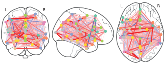
Figure 5: Controls using PLA-GGMs

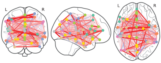
Figure 6: Patients using PLA-GGMs

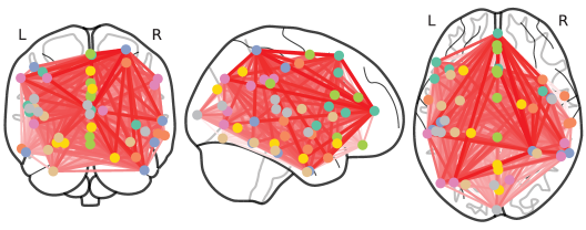
Figure 7: Controls using LR-GGMs

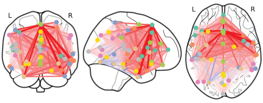
Figure 8: Patients using LR-GGMs

Schizophrenia Diagnosis using Different $\mathds{1}_{\left\{\absolutevalue{g}\geq g^{*}\right\}}$’s

We conduct the analysis in Section 6.2 using different $\mathds{1}_{\left\{\absolutevalue{g}\geq g^{*}\right\}}$’s. Specifically, we consider the function $1-\exp(-kx^{2})/2$ using $k=144,150$. The achieved accuracy using the parameter selected by the 10-fold cross validation and AIC are reported in Figure 9. The performance of PLA-GGMs is not hugely affected when selecting $\mathds{1}_{\left\{\absolutevalue{g}\geq g^{*}\right\}}$ in a reasonable range, which is consistent with our analysis in Theorem 1. Note that, if we select $k$ too large, the PPL method will be not applicable. The reason is that a large $k$ corresponds to a small $g^{*}$, and will induce few non-confounded samples observed. As a result, $\left(\mathbf{D}_{ij}^{\top}\mathbf{W}_{i}\mathbf{D}_{ij}\right)$ will be singular. In practice, if we use a relative large $g^{*}$ corresponding to a small $k$, (2) will tend to be like $\mathbf{R}(g)=0$ used in CON-GGMs and LR-GGMs.

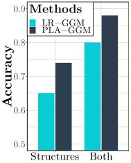
(a) $k=100$

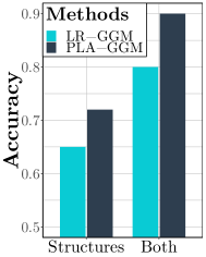
(b) $k=144$

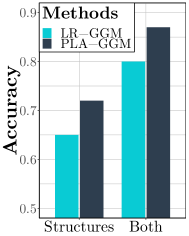
(c) $k=150$

Figure 9: Diagnosis using different $\mathds{1}_{\left\{\absolutevalue{g}\geq g^{*}\right\}}$’s.

References

- Andersen et al. (2018) Andersen, M., Winther, O., Hansen, L. K., Poldrack, R., and Koyejo, O. Bayesian structure learning for dynamic brain connectivity. In International Conference on Artificial Intelligence and Statistics, pp. 1436–1446, 2018.
- Arroyo-Relión et al. (2017) Arroyo-Relión, J. D., Kessler, D., Levina, E., and Taylor, S. F. Network classification with applications to brain connectomics. arXiv preprint arXiv:1701.08140, 2017.
- Barber & Kolar (2018) Barber, R. F. and Kolar, M. Rocket: Robust confidence intervals via kendall’s tau for transelliptical graphical models. Ann. Statist., 46(6B):3422–3450, 2018. ISSN 0090-5364. doi: 10.1214/17-AOS1663.
- Belilovsky et al. (2016) Belilovsky, E., Varoquaux, G., and Blaschko, M. B. Testing for differences in gaussian graphical models: applications to brain connectivity. In Advances in Neural Information Processing Systems, pp. 595–603, 2016.
- Biswal et al. (1995) Biswal, B., Zerrin Yetkin, F., Haughton, V. M., and Hyde, J. S. Functional connectivity in the motor cortex of resting human brain using echo-planar mri. Magnetic resonance in medicine, 34(4):537–541, 1995.
- Cheng et al. (2014) Cheng, G., Zhou, L., Huang, J. Z., et al. Efficient semiparametric estimation in generalized partially linear additive models for longitudinal/clustered data. Bernoulli, 20(1):141–163, 2014.
- Chouldechova & Hastie (2015) Chouldechova, A. and Hastie, T. Generalized additive model selection. arXiv preprint arXiv:1506.03850, 2015.
- COBRE (2019) COBRE. The center for biomedical research excellence. http://fcon_1000.projects.nitrc.org/indi/retro/cobre.html, 2019. (Accessed on 01/14/2019).
- Eaton (1983) Eaton, M. Multivariate statistics: a vector space approach. Lecture notes-monograph series. Institute of Mathematical Statistics, 1983. ISBN 9780940600690. URL https://books.google.com/books?id=WyvvAAAAMAAJ.
- Fan & Zhang (2008) Fan, J. and Zhang, W. Statistical methods with varying coefficient models. Statistics and its Interface, 1(1):179, 2008.
- Fan et al. (2005) Fan, J., Huang, T., et al. Profile likelihood inferences on semiparametric varying-coefficient partially linear models. Bernoulli, 11(6):1031–1057, 2005.
- Fox & Raichle (2007) Fox, M. D. and Raichle, M. E. Spontaneous fluctuations in brain activity observed with functional magnetic resonance imaging. Nature Reviews Neuroscience, 8(9):700–711, 2007.
- Friedman et al. (2008) Friedman, J., Hastie, T., and Tibshirani, R. Sparse inverse covariance estimation with the graphical lasso. Biostatistics, 9(3):432–441, 2008.
- Friedman et al. (2010) Friedman, J., Hastie, T., and Tibshirani, R. Regularization paths for generalized linear models via coordinate descent. Journal of Statistical Software, 33(1):1–22, 2010. URL http://www.jstatsoft.org/v33/i01/.
- Geng et al. (2017) Geng, S., Kuang, Z., and Page, D. An efficient pseudo-likelihood method for sparse binary pairwise markov network estimation. arXiv preprint arXiv:1702.08320, 2017.
- Geng et al. (2018a) Geng, S., Kolar, M., and Koyejo, O. Joint nonparametric precision matrix estimation with confounding. arXiv preprint arXiv:1810.07147, 2018a.
- Geng et al. (2018b) Geng, S., Kuang, Z., Liu, J., Wright, S., and Page, D. Stochastic learning for sparse discrete markov random fields with controlled gradient approximation error. In Uncertainty in artificial intelligence: proceedings of the… conference. Conference on Uncertainty in Artificial Intelligence, volume 2018, pp. 156. NIH Public Access, 2018b.
- Geng et al. (2018c) Geng, S., Kuang, Z., Peissig, P., and Page, D. Temporal poisson square root graphical models. In International Conference on Machine Learning, pp. 1700–1709, 2018c.
- Goto et al. (2016) Goto, M., Abe, O., Miyati, T., Yamasue, H., Gomi, T., and Takeda, T. Head motion and correction methods in resting-state functional mri. Magnetic Resonance in Medical Sciences, 15(2):178–186, 2016.
- Hastie (2017) Hastie, T. J. Generalized additive models. In Statistical models in S, pp. 249–307. Routledge, 2017.
- Huang et al. (2012) Huang, C.-Y., Qin, J., and Follmann, D. A. A maximum pseudo-profile likelihood estimator for the cox model under length-biased sampling. Biometrika, 99(1):199–210, 2012.
- Jordan (1998) Jordan, M. I. Learning in graphical models, volume 89. Springer Science & Business Media, 1998.
- Kolar & Xing (2011) Kolar, M. and Xing, E. On time varying undirected graphs. In Proc. of AISTATS, 2011.
- Kolar & Xing (2012) Kolar, M. and Xing, E. P. Estimating networks with jumps. Electron. J. Stat., 6:2069–2106, 2012. ISSN 1935-7524. doi: 10.1214/12-EJS739. URL https://doi.org/10.1214/12-EJS739.
- Kolar et al. (2009) Kolar, M., Song, L., and Xing, E. P. Sparsistent learning of varying-coefficient models with structural changes. In Advances in neural information processing systems, pp. 1006–1014, 2009.
- Kolar et al. (2010a) Kolar, M., Parikh, A. P., and Xing, E. P. On sparse nonparametric conditional covariance selection. In Fürnkranz, J. and Joachims, T. (eds.), Proceedings of the 27th International Conference on Machine Learning (ICML-10), June 21-24, 2010, Haifa, Israel, pp. 559–566. Omnipress, 2010a. URL https://icml.cc/Conferences/2010/papers/197.pdf.
- Kolar et al. (2010b) Kolar, M., Song, L., Ahmed, A., Xing, E. P., et al. Estimating time-varying networks. The Annals of Applied Statistics, 4(1):94–123, 2010b.
- Kuang et al. (2017) Kuang, Z., Geng, S., and Page, D. A screening rule for l1-regularized ising model estimation. In Advances in neural information processing systems, pp. 720–731, 2017.
- Laumann et al. (2016) Laumann, T. O., Snyder, A. Z., Mitra, A., Gordon, E. M., Gratton, C., Adeyemo, B., Gilmore, A. W., Nelson, S. M., Berg, J. J., Greene, D. J., et al. On the stability of bold fmri correlations. Cerebral cortex, 27(10):4719–4732, 2016.
- Laurent & Massart (2000) Laurent, B. and Massart, P. Adaptive estimation of a quadratic functional by model selection. Annals of Statistics, pp. 1302–1338, 2000.
- Lee & Liu (2015) Lee, W. and Liu, Y. Joint estimation of multiple precision matrices with common structures. The Journal of Machine Learning Research, 16(1):1035–1062, 2015.
- Liu et al. (2009) Liu, H., Lafferty, J., and Wasserman, L. The nonparanormal: Semiparametric estimation of high dimensional undirected graphs. Journal of Machine Learning Research, 10(Oct):2295–2328, 2009.
- Liu & Page (2013) Liu, J. and Page, D. Bayesian estimation of latently-grouped parameters in undirected graphical models. In Advances in neural information processing systems, pp. 1232–1240, 2013.
- Liu et al. (2014) Liu, J., Zhang, C., Burnside, E., and Page, D. Learning heterogeneous hidden markov random fields. In Artificial Intelligence and Statistics, pp. 576–584, 2014.
- Lou et al. (2016) Lou, Y., Bien, J., Caruana, R., and Gehrke, J. Sparse partially linear additive models. Journal of Computational and Graphical Statistics, 25(4):1126–1140, 2016.
- Lu et al. (2015) Lu, J., Kolar, M., and Liu, H. Kernel meets sieve: Post-regularization confidence bands for sparse additive model. arXiv preprint arXiv:1503.02978, 2015.
- Lu et al. (2018) Lu, J., Kolar, M., and Liu, H. Post-regularization inference for time-varying nonparanormal graphical models. Journal of Machine Learning Research, 18(203):1–78, 2018. URL http://jmlr.org/papers/v18/17-145.html.
- Mack & Silverman (1982) Mack, Y.-p. and Silverman, B. W. Weak and strong uniform consistency of kernel regression estimates. Zeitschrift für Wahrscheinlichkeitstheorie und verwandte Gebiete, 61(3):405–415, 1982.
- Meinshausen & Bühlmann (2006) Meinshausen, N. and Bühlmann, P. High-dimensional graphs and variable selection with the lasso. The annals of statistics, 34(3):1436–1462, 2006.
- Mignotte et al. (2000) Mignotte, M., Collet, C., Perez, P., and Bouthemy, P. Sonar image segmentation using an unsupervised hierarchical mrf model. IEEE transactions on image processing, 9(7):1216–1231, 2000.
- Ortega & Rheinboldt (2000) Ortega, J. M. and Rheinboldt, W. C. Iterative solution of nonlinear equations in several variables. SIAM, 2000.
- Patel et al. (2016) Patel, P., Aggarwal, P., and Gupta, A. Classification of schizophrenia versus normal subjects using deep learning. In Proceedings of the Tenth Indian Conference on Computer Vision, Graphics and Image Processing, pp. 28. ACM, 2016.
- Power et al. (2014) Power, J. D., Mitra, A., Laumann, T. O., Snyder, A. Z., Schlaggar, B. L., and Petersen, S. E. Methods to detect, characterize, and remove motion artifact in resting state fmri. Neuroimage, 84:320–341, 2014.
- Ravikumar et al. (2010) Ravikumar, P., Wainwright, M. J., Lafferty, J. D., et al. High-dimensional ising model selection using l1-regularized logistic regression. The Annals of Statistics, 38(3):1287–1319, 2010.
- Rothenhäusler et al. (2018) Rothenhäusler, D., Ernest, J., Bühlmann, P., et al. Causal inference in partially linear structural equation models. The Annals of Statistics, 46(6A):2904–2938, 2018.
- Shalizi & Thomas (2011) Shalizi, C. R. and Thomas, A. C. Homophily and contagion are generically confounded in observational social network studies. Sociological methods & research, 40(2):211–239, 2011.
- Sheffield et al. (2015) Sheffield, J. M., Repovs, G., Harms, M. P., Carter, C. S., Gold, J. M., MacDonald III, A. W., Ragland, J. D., Silverstein, S. M., Godwin, D., and Barch, D. M. Fronto-parietal and cingulo-opercular network integrity and cognition in health and schizophrenia. Neuropsychologia, 73:82–93, 2015.
- Shine et al. (2015) Shine, J. M., Koyejo, O., Bell, P. T., Gorgolewski, K. J., Gilat, M., and Poldrack, R. A. Estimation of dynamic functional connectivity using multiplication of temporal derivatives. NeuroImage, 122:399–407, 2015.
- Shine et al. (2016) Shine, J. M., Koyejo, O., and Poldrack, R. A. Temporal metastates are associated with differential patterns of time-resolved connectivity, network topology, and attention. Proceedings of the National Academy of Sciences, 113(35):9888–9891, 2016.
- Sohn & Kim (2012) Sohn, K.-A. and Kim, S. Joint estimation of structured sparsity and output structure in multiple-output regression via inverse-covariance regularization. In Artificial Intelligence and Statistics, pp. 1081–1089, 2012.
- Song et al. (2009a) Song, L., Kolar, M., and Xing, E. Keller: Estimating time-varying interactions between genes. Bioinformatics, 25(12):i128–i136, 2009a.
- Song et al. (2009b) Song, L., Kolar, M., and Xing, E. Time-varying dynamic bayesian networks. In Bengio, Y., Schuurmans, D., Lafferty, J. D., Williams, C. K. I., and Culotta, A. (eds.), Proc. of NIPS, pp. 1732–1740, 2009b.
- Speckman (1988) Speckman, P. Kernel smoothing in partial linear models. Journal of the Royal Statistical Society. Series B (Methodological), pp. 413–436, 1988.
- Suggala et al. (2017) Suggala, A., Kolar, M., and Ravikumar, P. K. The expxorcist: nonparametric graphical models via conditional exponential densities. In Advances in neural information processing systems, pp. 4446–4456, 2017.
- Tibshirani et al. (2012) Tibshirani, R., Bien, J., Friedman, J., Hastie, T., Simon, N., Taylor, J., and Tibshirani, R. J. Strong rules for discarding predictors in lasso-type problems. Journal of the Royal Statistical Society: Series B (Statistical Methodology), 74(2):245–266, 2012.
- Van Dijk et al. (2012) Van Dijk, K. R., Sabuncu, M. R., and Buckner, R. L. The influence of head motion on intrinsic functional connectivity mri. Neuroimage, 59(1):431–438, 2012.
- Voorman et al. (2013) Voorman, A., Shojaie, A., and Witten, D. Graph estimation with joint additive models. Biometrika, 101(1):85–101, 2013.
- Wainwright (2009) Wainwright, M. J. Sharp thresholds for high-dimensional and noisy sparsity recovery using -constrained quadratic programming (lasso). IEEE transactions on information theory, 55(5):2183–2202, 2009.
- Wang & Kolar (2014) Wang, J. and Kolar, M. Inference for sparse conditional precision matrices. ArXiv e-prints, arXiv:1412.7638, December 2014.
- Wytock & Kolter (2013) Wytock, M. and Kolter, Z. Sparse gaussian conditional random fields: Algorithms, theory, and application to energy forecasting. In International conference on machine learning, pp. 1265–1273, 2013.
- Yang & Ravikumar (2011) Yang, E. and Ravikumar, P. On the use of variational inference for learning discrete graphical model. In Getoor, L. and Scheffer, T. (eds.), Proceedings of the 28th International Conference on Machine Learning (ICML-11), ICML ’11, pp. 1009–1016, New York, NY, USA, June 2011. ACM. ISBN 978-1-4503-0619-5.
- Yang et al. (2015a) Yang, E., Ravikumar, P., Allen, G. I., and Liu, Z. Graphical models via univariate exponential family distributions. Journal of Machine Learning Research, 16(1):3813–3847, 2015a.
- Yang et al. (2015b) Yang, S., Lu, Z., Shen, X., Wonka, P., and Ye, J. Fused multiple graphical lasso. SIAM Journal on Optimization, 25(2):916–943, 2015b.
- Zhu & Cribben (2017) Zhu, Y. and Cribben, I. Graphical models for functional connectivity networks: best methods and the autocorrelation issue. bioRxiv, pp. 128488, 2017.
- Zhu & Koyejo (2018) Zhu, Y. and Koyejo, O. Clustered fused graphical lasso. In Conference on Uncertainty in Artificial Intelligence (UAI), 2018.