Transition to metallization in warm dense helium-hydrogen mixtures using stochastic density functional theory within the Kubo-Greenwood formalism

Abstract

The Kubo-Greenwood (KG) formula is often used in conjunction with Kohn-Sham (KS) density functional theory (DFT) to compute the optical conductivity, particularly for warm dense mater. For applying the KG formula, all KS eigenstates and eigenvalues up to an energy cutoff are required and thus the approach becomes expensive, especially for high temperatures and large systems, scaling cubically with both system size and temperature. Here, we develop an approach to calculate the KS conductivity within the stochastic DFT (sDFT) framework, which requires knowledge only of the KS Hamiltonian but not its eigenstates and values. We show that the computational effort associated with the method scales linearly with system size and reduces in proportion to the temperature unlike the cubic increase with traditional deterministic approaches. In addition, we find that the method allows an accurate description of the entire spectrum, including the high-frequency range, unlike the deterministic method which is compelled to introduce a high-frequency cut-off due to memory and computational time constraints. We apply the method to helium-hydrogen mixtures in the warm dense matter regime at temperatures of $\sim 60\text{kK}$ and find that the system displays two conductivity phases, where a transition from non-metal to metal occurs when hydrogen atoms constitute $\sim 0.3$ of the total atoms in the system.

I Introduction

The state of warm dense matter (WDM) is characterized by high atomic density, similar to conventional condensed matter systems, and elevated temperatures of several electron volts ($1\text{eV}\approx 10^{4}K$). This is an intermediate regime bridging plasma physics and condensed matter physics for which equations of state (EOS) and other properties are of interest. One example appears in the study of hydrogen-helium mixtures under extreme conditions, where the EOS (Militzer, 2013), phase separation and physical properties, such as conductivity (Lorenzen et al., 2011) and miscibility (Schöttler and Redmer, 2018) can be used to explain the luminosity and gravitational moments of planets such as Jupiter and other gas giants, as well as their formation and evolution characteristics (Stevenson, 1975; Nettelmann et al., 2008; Guillot, 1999). Generally, EOS and properties are calculated for various materials using first-principle methods, specifically the Kohn-Sham density functional theory (KS-DFT) at finite temperatures (Silvestrelli et al., 1996; Mattsson and Wahnstrom, 1997; Pozzo et al., 2012; Witte et al., 2018), often showing good agreement with experiments (Witte et al., 2018; Holst et al., 2008; Preising et al., 2018). Within the KS-DFT framework, WDM conductivity is often obtained by using the Kubo-Greenwood (KG) formalism (Kubo, 1957; Mazevet et al., 2010; Holst et al., 2011; Desjarlais et al., 2002) with good results when compared to experiment. The KS-DFT and the KG electrical conductivity equation when applied to WDM requires large computational effort which increases dramatically with temperature and system size, because of the need to construct and propagate all the occupied KS eigenstates, as well as a sufficient number of unoccupied states, the number of which grows as $T^{3}$, where $T$ is the temperature (Cytter et al., 2018)).

Recently, stochastic DFT (sDFT) approaches that circumvent the computational difficulties mentioned above have been developed (Baer et al., 2013; Neuhauser et al., 2014; Cytter et al., 2014, 2018; Fabian et al., 2018; Chen et al., 2019) for ground/thermal state calculations. These have also served as a basis for developing time-dependent methodologies for description of materials properties (Gao et al., 2015; Neuhauser et al., 2017; Hernandez et al., 2018; Takeshita et al., 2017). It was shown that sDFT is especially useful for EOS calculations in the WDM regime since it involves a computational effort that scales as $T^{-1}$ (Cytter et al., 2018).

In this paper, we develop an approach for calculating the KG conductivity within the framework of sDFT. The main advantage of the approach is that it does not require any knowledge of the occupied or empty KS orbitals. We show and benchmark a stochastic method to sample the KG conductivity. We then use the method to study the conductivity in hydrogen-helium mixtures. Our approach is similar to previously developed stochastic conductivity approaches (Wang, 1994; Baer et al., 2004; Iitaka et al., 1997) but differs in essential implementation details and is unique in its combination with sDFT calculations.

In the paper, we present the development of the stochastic KG (sKG) method and provide important implementation details, as well as demonstrations of the methods validity and a discussion in the statistical errors and scaling in Sec. II. In Sec. III the sDFT-sKG method is applied to the study of the conductivity of mixtures helium and hydrogen in the warm dense matter regime, targeting metallization and beyond-linear-mixing effects.

II Method

II.1 Time-dependent linear response

The time-dependent expectation value of a many-body observable $\hat{B}$ after an impulsive perturbation is applied through the observable $\hat{A}$ to a system at time $t=0$ (usually assumed in thermal equilibrium) is given, in the linear-response regime, as the following correlation function (Kubo, 1957, 1966): $C_{AB}\left(t\right)=i\theta\left(t\right)\text{Tr}\left[\rho\left(\beta,\mu\right)\left[\hat{A},\hat{B}\left(t\right)\right]\right]$ where $\hat{B}\left(t\right)=e^{i\hat{H}t/\hbar}\hat{B}e^{-i\hat{H}t/\hbar}$, $\hat{H}$ is the unperturbed Hamiltonian and $\theta\left(t\right)$ is the Heaviside function imposing causality. The expectation values are performed with respect to the many-body thermal density $\rho\left(\beta,\mu\right)=Z\left(\beta,\mu\right)^{-1}e^{-\beta\left(\hat{H}-\mu\hat{N}\right)}$ where $Z\left(\beta,\mu\right)$ is the partition function at chemical potential $\mu$ and inverse temperature $\beta=\frac{1}{k_{B}T}$, $k_{B}$ being the Boltzmann constant.

One of the important applications of linear-response theory is the prediction of the frequency-dependent conductivity

$$\sigma(\omega)=\frac{2\pi e^{2}}{\Omega m_{e}^{2}\hbar}\frac{\Im\left(\tilde{C}_{PP}(\omega)\right)}{\omega}$$ (1)

where $\Omega$ is the volume of the simulation cell and $\tilde{C}_{PP}(\omega)$ is the Fourier transform of the momentum-momentum correlation function,

$$\tilde{C}_{PP}\left(\omega\right)=\int_{0}^{\infty}C_{PP}\left(t\right)e^{-i\omega t}e^{-\frac{1}{2}\eta^{2}t^{2}}dt,$$ (2)

and $\eta$ is a small real parameter. In the limit $\omega\to 0$ L’hopital’s rule can be used to assess the DC conductivity:

$$\sigma\left(0\right)=\frac{2\pi e^{2}}{\Omega m_{e}^{2}\hbar}\lim_{\omega\to 0}\frac{\partial\Im\tilde{C}_{PP}\left(\omega\right)}{\partial\omega}.$$ (3)

For non-interacting particles, with a single-particle Hamiltonian $\hat{h}$, having eigenvalues $\varepsilon_{n}$ and eigenstates $\left|n\right\rangle$, $n=1,2,...$, the correlation function reduces to the following expression:

$$C_{AB}\left(t\right)=-2\theta\left(t\right)\Im\text{Tr}\left[f_{FD}\left(\hat{h}\right)\hat{a}\left(1-f_{FD}\left(\hat{h}\right)\right)\hat{b}\left(t\right)\right]$$ (4)

where $\hat{a}$, $\hat{b}$ are the single-particle perturbing and observed operators, respectively, $\hat{b}\left(t\right)=e^{i\hat{h}t}\hat{b}e^{-i\hat{h}t}$ and

$$f_{FD}\left(\hat{h}\right)\equiv\frac{1}{1+e^{\beta\left(\hat{h}-\mu\right)}}$$ (5)

is the Fermi-Dirac distribution. Combining Eq. 4 and Eq. 2 and taking the formal limit $\eta\rightarrow 0$ gives the Kubo-Greenwood (KG) conductivity (Kubo, 1957; Greenwood, 1958):

$$\sigma\left(\omega\right)=\frac{2\pi e^{2}}{\Omega m_{e}^{2}\hbar\omega}\sum_{m,n}^{N_{g}}f_{mn}\left|p_{mn}\right|^{2}\delta\left(\omega-\varepsilon_{nm}/\hbar\right),$$ (6)

where $N_{g}$ is the number of grid points, $f_{mn}\equiv f_{FD}\left(\varepsilon_{m}\right)-f_{FD}\left(\varepsilon_{n}\right)$, $\varepsilon_{nm}=\varepsilon_{n}-\varepsilon_{m}$ and $p_{nm}=\left\langle n\left|\hat{p}\right|m\right\rangle$. For practical reasons, the summation over the occupied and unoccupied states is determined according to an energy cutoff and as a result the conductivity spectrum can be calculated only up to a corresponding frequency cutoff.

II.2 Stochastic calculation of the response function

To calculate the KG conductivity in a stochastic manner the stochastic trace formula (Hutchinson, 1990) can be used to estimate the trace in Eq. (4). However, we found that a smaller statistical noise can be obtained if the stochastic trace is applied to following equivalent but more symmetrical expression:

$$C_{PP}\left(t\right)=-2\theta\left(t\right)\Im\text{Tr}\left[\sqrt{f_{FD}}\hat{p}\left(1-f_{FD}\right)\hat{p}\left(t\right)\sqrt{f_{FD}}\right].$$ (7)

To apply the stochastic trace formula, we define a set of stochastic orbitals $\chi$, represented on the grid such that $\left\langle\boldsymbol{r}_{g}|\chi_{i}\right\rangle=\left(\delta x\right)^{-3/2}e^{i\theta_{g}^{i}}$, where $\theta_{g}\in\left[0,2\pi\right]$ is a random phase and $\delta x$ is the grid spacing.The stochastic expression for $C_{PP}\left(t\right)$ is given by:

$$C_{PP}\left(t\right) =-2\theta\left(t\right)\text{E}\left\{\Im\left\langle\xi\left|\hat{p}\left(1-f_{FD}\left(\hat{h}\right)\right)e^{i\hat{h}t}\hat{p}e^{-i\hat{h}t}\right|\xi\right\rangle\right\},$$ (8)

where $\left|\xi\right\rangle=\sqrt{f_{FD}\left(\hat{h}\right)}\left|\chi\right\rangle$ and $\text{E}\left\{...\right\}$ designates an expectation value.

The procedure consists of the following schematic steps:

1. Set: $n=0$, $\left|\eta_{j}\right\rangle=\left|\xi_{j}\right\rangle$, $\left|\zeta_{j}\right\rangle=\left(1-f_{FD}\left(\hat{h}\right)\right)\hat{p}\left|\xi_{j}\right\rangle$, and the time-step $\Delta t=\frac{\pi}{\Delta E}$, where $\Delta E=E_{max}-E_{min}$ and $E_{max}$ ($E_{min})$ is the maximal (minimal) eigenvalue of $\hat{h}$ (the condition is required to avoid aliasing). The time step determines the cutoff frequency of the spectrum and $N_{ts}=\frac{\Delta E}{\Delta\omega}=\frac{\pi}{\Delta\omega\Delta t}$ is the total number of time steps for achieving a spectral resolution of $\Delta\omega$.

2. Calculate: $C_{PP}^{j}\left(n\Delta t\right)=-2\Im\left\langle\zeta_{j}\left|\hat{p}\right|\eta_{j}\right\rangle$.

3. Set $n=n+1$ , $\left|\eta_{j}\right\rangle=e^{-i\hat{h}\Delta t}\left|\eta_{j}\right\rangle$, $\left|\zeta_{j}\right\rangle=e^{-i\hat{h}\Delta t}\left|\zeta_{j}\right\rangle$.

4. Go to 2 and repeat until $n=N_{ts}$.

5. The response function is then averaged over $I_{\sigma}$ (the number of stochastic orbitals), yielding $C_{PP}\left(n\Delta t\right)\approx\frac{1}{I_{\sigma}}\sum_{j=1}^{I_{\sigma}}C_{PP}^{j}\left(n\Delta t\right)$. This response function is then discrete-Fourier transformed and used to obtain the frequency-dependent conductivity (Eq. (1)).

The process is easily parallelized, since each element $C_{PP}^{j}\left(n\Delta t\right)$ is calculated independently before averaging in the final step. In our calculations we do not use the above procedure directly because using Chebyshev expansions for the evolution operator, we found a way to expedite the calculation as described in Sec. II.5.

The stochastic-KG (sKG) procedure forms a post processing step after a sDFT calculation (Baer et al., 2013; Cytter et al., 2018) which provides the self consistent KS Hamiltonian $\hat{h}$. The stochastic calculation requires two sets of stochastic orbitals, one set is used to perform sDFT calculation with which $\hat{h}$ is determined, this set will be denoted “sDFT-os” and a second set, used in the sKG calculation to determine the conductivity is denoted “sKG-os”. The KS wave functions are expanded using plane waves although the non-local part of the pseudopotentials are implemented using a real-space grid, for achieving high efficiency. For all the stochastic calculations in this paper, we used the local density approximation (LDA) (Perdew and Wang, 1992) and Troullier-Martins norm-conserving pseudopotentials (Troullier and Martins, 1991) within the Kleinman-Bylander representation (Kleinman and Bylander, 1982).

II.3 Validation of the method

To validate the method we compare conductivity estimates with that of the well-established Quantum Espresso (QE) package (Giannozzi et al., 2009), for carrying out both the DFT and the KG (using the KGEC module (Calderín et al., 2017)) calculations. The results for $\text{H}_{256}$ (at $4000K$) and a single He atom (at $3200K$) are shown in the panels of Fig. 1 and the density of states (DOS) $\rho\left(\varepsilon\right)$, is shown in the insets. The $\text{H}_{256}$ nuclear configuration was obtained using an AIMD simulation using VASP. It can be seen that for both systems the stochastic conductivity spectra and the DOS curves are in close agreement with the corresponding deterministic estimates of QE throughout the entire frequency/energy range.

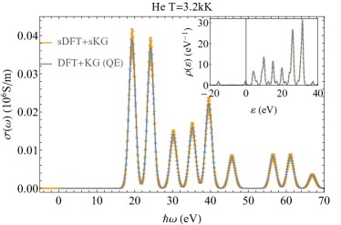
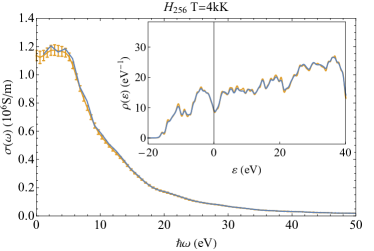
Figure 1: The conductivity $\sigma\left(\omega\right)$ and DOS $\rho\left(\varepsilon\right)$ (in the insets) using stochastic versus deterministic (Quantum Espresso) calculations. We show two examples, each calculated in a periodic simulation cell of length $L$ at the $\Gamma$-point: an insulator He atom at $3200K$ with $L=5.3\textup{\AA}$ (upper panel) and a metallic system, $\text{H}_{256}$ at $4000K$, with $L=8\textup{\AA}$ (lower panel). The deterministic QE results used $200$ KS eigenstates for the first system and $1700$ for the second. For the stochastic DFT calculation we used 960 stochastic orbitals for the insulator and 480 orbitals for the conductor. The conductivity of both systems was calculated using $120$ stochastic orbitals. A kinetic energy cutoff of $762\;\text{eV}$ for He and $525$ eV for $\text{H}_{256}$ was used. Each peak was Gaussian-broadened, deploying a width parameter equal to $\eta=1.2\text{eV}$ (in sKG this parameter affects Eq. 2).

To further test the method we also looked at $\text{He}_{128}$ systems in the temperature range $27-57\text{kK}$ and density range $0.71-0.83\frac{\text{g}}{\text{cm}^{3}}$ respectively. To obtain a set of nuclear configurations, an ab initio molecular dynamics (AIMD) trajectory was run using the PBE (Perdew et al., 1996) exchange-correlation (XC) functional, employing the plane-wave code VASP (Hafner, 2007; Kresse and Furthmuller, 1996). Snapshots of the nuclear configurations were then taken from the equilibrated part of the simulation, as described in Ref. 12. For each snapshot we performed a sDFT calculation using 160 sDFT-os to obtain the Hamiltonian. The standard deviation was estimated by using five different sets of 160 sKG-os, each different from the set used for the Hamiltonian calculation, to avoid bias. For a given nuclear snapshots, the stochastic calculation produces a conductivity spectrum with certain stochastic error. The stochastic fluctuations in our case, turned out to be larger than the fluctuations arising from averaging over the different nuclear configurations. We therefore present here results obtained from one snapshot only. To calculate the discretized momentum-momentum correlation function $C_{PP}\left(\Delta t\times n\right)$ we used $n=600$ time-steps with $\Delta t=0.25\,\hbar E_{h}^{-1}$. The conductivity spectrum is then obtained from Eq. 8 using a Gaussian broadening parameter of $\eta=0.036\text{eV}$.

The full spectrum and the standard deviation involved in the calculation as described above are shown in Fig. 2. The advantage of the stochastic method is apparent when looking at frequencies higher than $\sim 70\leavevmode\nobreak\ eV$, where the deterministic calculation of Ref. 12, gives no contributions above this cut-off energy which has to be introduced in plane-wave DFT codes like VASP. The deterministic frequency range could have increased in principle by including more KS states, but this would require an excessive computational effort. Careful analysis with respect to the cut-off energy show that equation-of-state data and the low-frequency conductivity can be converged properly (see e.g. Refs. (Holst et al., 2008; Preising et al., 2018)). The sKG calculation on the other hand samples states from the entire energy spectrum and therefore exhibits the physically correct asymptotic decay of $\omega^{-5/2}$, as expected for the free electron gas. The correct high-frequency asymptotic behavior enables calculation of the Thomas-Reiche-Kuhn sum-rule (Kuhn, 1925; Reiche and Thomas, 1925) which states that the total oscillator strength per electron $f_{osc}/N_{e}$, where

$$f_{osc}=\frac{m_{e}\Omega}{\pi e^{2}}\int_{-\infty}^{\infty}\sigma\left(\omega\right)d\omega,$$ (9)

and $\sigma\left(\omega\right)$ is the conductivity defined in Eq. (1), should be equal to 1. The actual calculated values of $f_{osc}/N_{e}$ are shown in Table 1 for three $\text{He}_{128}$ systems (one of which we considered in Fig. 2 and two others, of different temperature and densities are given for further demonstration) and are indeed very close to the theoretical value of 1, signifying that the calculations are converged with respect to the number of states and the total time of propagation.

At intermediate frequencies, we find (Fig. 2) a close overall agreement between the deterministic and stochastic estimates of the conductivity spectra, despite the fact that both methods make use of different XC functionals. The most conspicuous feature of the spectrum in this range is its peak at $\hbar\omega_{peak}\approx 25\text{eV}$, featuring the maximal deviation between the two spectra which is nonetheless small, with a 10% difference in height and 0.3eV difference in the value of $\hbar\omega_{peak}$.

The DC conductivity for three different systems are displayed in the third and fourth columns of Table 1 and the agreement between the deterministic and stochastic zero frequency limit is shown.

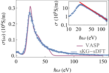
Figure 2: The conductivity spectrum for a $\text{He}_{128}$ system at $T=27\text{kK}$ and density of $0.83\frac{\text{g}}{\text{cm}^{3}}$. The sKG-sDFT LDA conductivity with error bars (with $I_{\sigma}=I_{H}=160$) is compared to the deterministic results by VASP based on PBE, as described in Ref. 12. The deterministic calculations were done with an energy cutoff of $800\text{eV}$ using 570 KS-states. Inset: The spectrum decay. the red line is proportional to $\omega^{-5/2}$.

System		$f_{osc}/N_{e}$	$\sigma_{DC}\left(10^{6}\text{Siemens}/m\right)$
$\rho/(\text{g}/\text{cm}^{3})$	$T/kK$		VASP/PBE	sKG-sDFT/LDA
$0.71$	29	1.010	$0.021\pm 0.001$	$0.026\pm 0.002$
$0.83$	27	0.998	$0.018\pm 0.001$	$0.02\pm 0.003$
0.75	57	1.014	$0.110\pm 0.002$	$0.10\pm 0.02$0

Table 1: The total oscillator strength per electron $f_{osc}/N_{e}$ (see Eq.9) and the DC conductivity calculated using VASP based on PBE (Preising et al., 2018) and the sDFT-sKG based on LDA employing $I_{\sigma}=I_{H}=160$ stochastic orbitals. The statistics for the stochastic calculation is obtained from 5 different sKG runs and that of the deterministic calculation was taken from 5 points in the proximity of the DC conductivity to evaluate the $\omega\rightarrow 0$ limit.

II.4 Analysis of the statistical errors

There are three sources of statistical errors in the calculation. The sDFT, that produces the Hamiltonian with which the conductivity is calculated by Eq. (2)-(3) contributes two of the errors. One is the fluctuation which is measured by the standard deviation of the results, and is proportional to $I_{H}^{-1/2}$, where $I_{H}$ is the number sDFT-os. The second is the bias, related to the deviance of the average from the exact value, discussed in previous works (Cytter et al., 2018; Fabian et al., 2018) that is proportional to $I_{H}^{-1}$. In addition to the errors in the sDFT stage, the stochastic evaluation of the momentum-momentum correlation function also contributes an additional fluctuation. The effect of the two errors arising from the sDFT calculation on the conductivity spectrum is displayed at the bottom panel of Fig. 3. We show three spectra, each based on a distinct sDFT Hamiltonian, calculated using different values of $I_{H}$. For the case of $I_{H}=150$ ten different sDFT-o sets were used in order to asses the fluctuation stemming from the stochastic procedure. For all three conductivity calculations, we used the same set of $I_{\sigma}=150$ sKG-os, thereby leading to a similar fluctuation, so that we can focus on the errors resulting from the sDFT process. The spectra based on $I_{H}=300$ are within the error bars of the $I_{H}=150$ for all frequencies considered, while the spectrum that is based on $I_{H}=75$ exhibits a deviation from the other two, especially near the $\omega\sim 25eV$ peak. Since the fluctuation is small, we deduce that this difference can be attributed to the bias component of the statistical error, and that it is small at $I_{H}=75$ and much smaller than the fluctuation when $I_{H}\geq 150$.

Having discussed the two errors connected with the stochastic nature of the Hamiltonian, we now address the random fluctuations that arise from the sKG calculation. For this purpose, we take one of the sDFT Hamiltonians above (that was calculated using $I_{H}=150$ sDFT-os) and perform three conductivity spectra calculations on it using different values $I_{\sigma}$ of sKG-os. The resulting spectra are shown in the uper panel of Fig. 3. The inset shows that the standard deviation, averaged over all frequencies, decreases according to the central limit theorem as expected. Since the sKG-os are used to directly sample the trace, the statistical error should be a “pure” fluctuation, with no bias. Therefore, while the peak in this example exhibits a decrease as $I_{\sigma}$ increases, we attribute that behavior to a fluctuation.

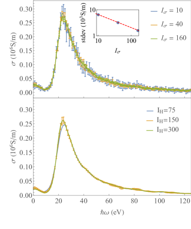
Figure 3: The conductivity spectrum of $\text{He}_{128}$ at 27kK and density of $0.83\text{g/$\text{cm}^{3}$}$. Top panel: The conductivity based on one sDFT Hamiltonian (using $I_{H}=150$) calculated with an increasing number $I_{\sigma}$ of sKG-os. Inset: The standard deviation (stdev) of the conductivity, averaged over all frequencies as a function of $I_{\sigma}$. The dashed line is proportional to $I_{\sigma}^{-1/2}$. Bottom panel: The conductivity based on three sDFT Hamiltonians, each obtained using $I_{H}$ sDFT-os. In order not to clutter the plot, error bars are given only for the $I_{H}=150$ sDFT-o’s calculation. The sKG calculations were all done using $I_{\sigma}=150$ sKG-os.

II.5 Algorithmic implementation and scaling of the algorithm

The computational time of the sKG algorithm, as described in subsection II.2 and Eq. (7) is determined mainly by application of $f_{FD}\left(\hat{h}\right)$, $\sqrt{f_{FD}\left(\hat{h}\right)}$ and the time evolution operator $e^{-i\hat{h}\Delta t}$, all functions of the Hamiltonian $\hat{h}$ on given wave-functions. Each of these Hamiltonian functions can be applied by using Chebyshev expansions (Kosloff, 1988; Goedecker and Colombo, 1994; Huang et al., 1995; Baer and Head-Gordon, 1997a), where the Hamiltonian is applied to the wave function repeatedly $N_{C}$ times. The length of the expansion $N_{C}$ is proportional to $\Delta E=E_{max}-E_{min}$ where $E_{max}$ and $E_{min}$ are upper and lower bounds on the maximal and minimal eigenvalues of $\hat{h}$ respectively. For the Fermi-Dirac functions $f_{FD}\left(\hat{h}\right)$ and $\sqrt{f_{FD}\left(\hat{h}\right)}$ the Chebyshev expansion length $N_{C}$ is proportional to $\beta\Delta E$.

Propagating the wave function $\varphi$ to different times can be performed with several Chebyshev expansions:

$$\varphi_{n}=e^{-i\hat{h}\left(n\Delta t\right)}\varphi=\sum_{m=0}^{N_{C}\left(n\Delta t\right)}a_{m}\left(n\Delta t\right)\phi_{m},$$ (10)

where $\phi_{m}$ are the Chebyshev recursion wave functions . Note that $\varphi_{n}$ for the different values of $n$ are different linear combinations of the same recursion wave functions $\phi_{m}$, but summed with different expansion coefficient $a_{m}\left(n\Delta t\right)$. We can therefore generate one set of $\phi_{1},\dots,\phi_{N_{C}}$ for generating the required set of $\varphi_{n}^{\prime}s$. The Chebyshev expansion length $N_{C}$ is determined as the smallest integer for which $\left|a_{m}\left(n\Delta t\right)\right|<10^{-9}$ for all $m\geq N_{C}$. Clearly, $N_{C}$ depends on $n\Delta t$, hence the notation $N_{C}\left(n\Delta t\right)$. The expansions in Eq. (10) are highly beneficial since most of the computational effort goes to applying the Hamiltonian on the different wave-functions, that is, calculating the set of $\phi^{\prime}s$. Thus, to find the optimized number of simultaneously calculated time-steps $n$, in Fig. 4 we look at the number of Chebyshev terms required per time step, $N_{C}\left(n\Delta t\right)/n$, along side the wall time for every choice of $n$. It can be seen that $N_{C}\left(n\Delta t\right)/n$ is highest at $n=1$ and as $n$ increases, its value drops steeply towards an asymptotic plateau value smaller by a factor of $\backsim 4$. It is seen that using this approach CPU times indeed decrease but due to an additional overhead of the calculation only a factor of 2 is obtained.

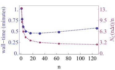
Figure 4: The CPU time (blue circled markers) and $N_{C}\left(n\Delta t\right)/n$ (purple square markers) as a function of the number $n$ of time step propagation operators used in the calculation. The calculation was done for $\text{He}_{128}$ using $N_{g}=60^{3}$ grid points, at $57\text{kK}$ on 8 processors where $N_{ts}=128$ and $\Delta t=0.25au$, for one dipole direction.

The computational effort for the sKG procedure has a near-linear scaling with system size $N$ as does the sDFT , and this is due to the following two reasons: 1) the Hamiltonian $\hat{h}$ action on a wave function involves a $O\left(N_{g}\ln N_{g}\right)$ numerical complexity (this is the operation count of the fast Fourier transform involved in the kinetic energy operation), where $N_{g}\propto N$ is the number of grid-points; and 2) The number of such Hamiltonian operations is $N_{C}\times I_{\sigma}$, where $N_{C}$ (the Chebyshev expansion length) and $I_{\sigma}$ (the number of sKG-os) are both system-size independent. For the same reasons t the sDFT calculation also scales linearly with $N$ (as shown before in Ref. 18). Furthermore, the computational effort in sDFT decreases as the temperature increases in proportion to $1/T$ (Cytter et al., 2018), due to the fact that the FD Chebyshev expansion length $N_{C}$ is proportional to $\Delta E/k_{B}T$ (Baer and Head-Gordon, 1997b) and the energy range $\Delta E$ is system-size independent. The $O\left(N/T\right)$ scaling with system size and temperature we report here should be compared to the $O\left(N^{3}T^{3}\right)$ scaling of the deterministic calculation based on Eq. (6), which requires calculation of all the occupied (and many unoccupied) states, the number of which is proportional to $T^{3}$ (based on the electron gas density of states). The system-size scaling can be seen in actual calculation, as shown in Fig.  5, where the wall-time for the DFT+KG calculation, is shown as a function of the number of atoms in the system (keeping the density and temperature fixed as the number of atoms increases) for deterministic (using QE) and sDFT+sKG. For small system sizes the QE calculation is considerably faster than the stochastic approach. However, as the system size increases, due to liner scaling, the stochastic approach becomes competitive. At $N=128$ we find a crossover and already for $N=432$ the stochastic calculation is 10 times faster than the deterministic one.

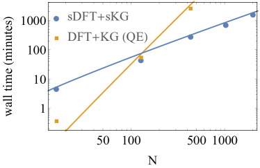
Figure 5: Wall time for stochastic DFT+KG calculations with 600 time steps with $\Delta t=0.25\,\hbar E_{h}^{-1}$ as well as a deterministic calculation done using Quantum Espresso (QE), as a function of the number of He atoms, at $0.75\frac{\text{g}}{\text{cm}^{3}}$ and 57kK. The orange curve is proportional to $N^{3}$, and the blue curve is linear with $N$, the number of atoms.

III Mixed He/H WDM systems

As an application of the method, we study the conductivity and DOS of various systems with different hydrogen-helium mixtures at temperature of $57\text{kK}$ and constant volume. For each system, we obtained a set of thermally-distributed nuclear configurations using the electron force-field (eFF) (Jaramillo-Botero et al., 2010) dynamics as implemented in LAMMPS (Plimpton, 1995), which has been shown has been shown to give a good description of the pair correlation and equations of state of first-row materials under extreme conditions (Kim et al., 2011; Su and Goddard, 2007). For $\text{He}_{128}$ at $57\text{kK}$ we generate a set of Boltzmann-distributed configurations using both an empirical force field and an ab-inito approach taken from Ref. 12. The configurations where then used to average the results over the thermal fluctuations of the nuclei. In Fig. 6 we compare the two sets of results and show that while giving two visibly different spectra they share similar trends with peaks/troughs located at nearly identical frequencies. Comparing the two DOSs we see small differences in the occupied state energies while being nearly identical at the unoccupied state energies. Comparing the correlation functions $g\left(r\right)$, we find that AIMD gives significant weight to He pairs approaching as close as $0.5\textup{\AA}$ while the eFF does not. Both functions show a peak at $1.1\textup{\AA}$, but it is more significant in AIMD. It is perhaps surprising that despite the rather large differences in the pair correlation between the two methods, the electronic properties, as mentioned above, are not very different.

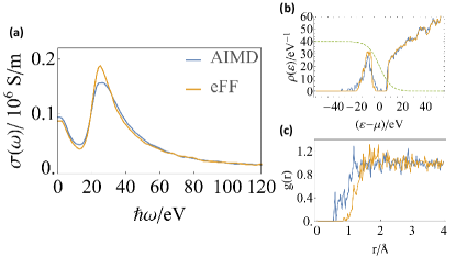
Figure 6: Comparison of the calculated conductivity $\sigma\left(\omega\right)$ (a), the DOS $\rho\left(\varepsilon\right)$ (b) and the radial pair correlation $g\left(r\right)$ (c) for $\text{He}_{128}$ at 57kK and density of $0.75\frac{\text{g}}{\text{cm}^{3}}$ based on configurations generated by AIMD (Preising et al., 2018) vs. eFF dynamics. The dashed line in panel (b) shows the Fermi-Dirac level occupation, transiting from a value of 1 at low energies $\varepsilon$ to $0$ at high energies .

We characterize the mixture by the hydrogen fraction in the system

$$X_{\text{H}}=\frac{N_{\text{H}}}{N_{\text{H}}+N_{\text{He}}}\ ,$$ (11)

where $N_{\text{H}}$ and $N_{\text{He}}$ are the number of hydrogen and helium atoms, respectively. For practical purposes, this ratio is achieved by holding the total number of atoms $N_{\text{H}}+N_{\text{He}}$ in the simulation cell constant and equal to $1024$.

We ran five molecular dynamics trajectories at fixed volume (minimum image periodic boundary conditions for $L=39.4\,a_{0}$) and temperature ($T=57\text{kK}$) with interactions between He and H described by the eFF force-field with a cutoff of 6.45$a_{0}$. Each trajectory started with the same ordered configuration, and a different velocity allocation, equilibrated, and then ran for a total of 3ps with time step of $10^{-3}\text{fs}$, needed due to consideration of both electronic and nuclear time scales. The duration of the trajectories corresponded to the correlation time of 3ps estimated using the same data. The final nuclear configuration for each trajectory represented a set of five uncorrelated H-He mixtures. For each structure, a sDFT calculation determined the Hamiltonian $\hat{h}$ which was used for the sKG calculation of the conductivity spectrum. For both sDFT and sKG an identical simulation box and grid of $N_{g}=120^{3}$ points was used which correspond to a grid spacing of $\delta x=0.33\;a_{0}$. The sDFT calculation was based on $I_{H}=120$ sDFT-o’s and the sKG calculation used a distinct set of $I_{\sigma}=120$ sKG-o’s.

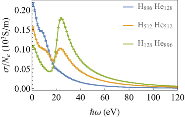
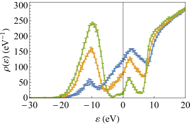
Figure 7: The Conductivity (upper panel) and the DOS (lower panel) of different systems containing 1024 atoms with different hydrogen percentages at $T=57\text{kK}$ and an average atomic volume of $60\,a_{0}^{3}$ per atom. The conductivity was normalized according to the number of electrons in the system. The DOS is shifted so that the chemical potential is zero.

In Fig. 7 the conductivity spectra and the density of states (DOS) for three different mixtures is displayed. These two characteristics are closely related and will therefore be discussed together. The statistical fluctuation in the DOS (lower panel), denoted as error bars, was determined by running sDFT calculations on the five distinct configuration snapshots as described above, each using a different set of sDFT-o’s. These five Hamiltonians were then used for evaluating the conductivity (upper panel) employing a different set of sKG-o’s to avoid additional bias. The resulting five conductance spectra and DOS were used for estimating the thermally-averaged curves and their associated statistical errors. It is seen in the upper panel of Fig. 7, that the statistical fluctuations are small compared to the difference between the curves and they do not seem to increase as a function of the hydrogen atomic fraction $X_{H}$ and therefore, only one snapshot was used in all other calculations.

When a relatively small fraction of hydrogen atoms is present in the system, it gives rise to a small peak at 3eV inside the Helium energy gap in the DOS (see the lower panel of Fig. 7). As the hydrogen concentration increases the He gap fills with states until it is no longer visible and at the same time the DOS of the valence band (seen in the figure at around $-10\text{eV}$), decreases steadily. Both effects show a gradual transition to metallization as the hydrogen ratio grows. At high energies the DOS of all mixtures converges to the free electron limit.

The sKG conductivity follows the changes seen in the DOS. Consider first the DC conductivity, shown in the lower panel of Fig. 8, which remains relatively constant as the hydrogen fraction grows until $X_{H}^{crit}\sim 0.3$. Beyond this value of the hydrogen fraction the DC conductivity increases near-linearly with $\chi_{\text{H}}$ as a result of the energy gap filling in the DOS, allowing more transitions at low energies. Due to the finite temperature and therefore partial occupation there exists zero frequency transitions even at helium dominated systems causing the DC conductivity to change only by a factor of 2.5 when moving from pure helium to pure hydrogen systems. The peak in the He dominated spectrum, as seen in the upper panel of Fig. 7, appears at around $25\text{eV}$ and corresponds to the transition from the highest density in the occupied band to the non-occupied band threshold levels (as seen in the DOS at $10\text{eV}$). Furthermore, at higher He concentrations due to the energy gap, transitions in 15eV become less probable, resulting in a local minimum in the conductivity at this frequency.

Next, we consider the frequency $\omega_{max}$ for which the conductivity is maximal, plotted as a function of $X_{H}$ in the top panel of Fig. 8. This frequency displays an abrupt shift of $\omega_{max}$ from $\sim 25\text{eV}$ to $0$ (DC) as $X_{H}$ passes through the critical value of $X_{H}^{crit}\sim 0.3$. This critical value, indicates an abrupt nonmetal-to-metal transition in the H-He system as reported in Ref. 2 for considerably lower temperatures. This critical hydrogen concentration is well withing the range of the Mott criterion for metallization in pure hydrogen, as seen in Ref. 53 that shows it occurs at $n_{H}^{1/3}a_{0}\approx 0.25$ for temperatures up to 15kK. In the present system, we find the metallization density at $n_{H}^{1/3}a_{0}\approx 0.18$, which seems reasonable considering the fact that we’re looking at a substantially higher temperature in which thermal effects promote the conductivity onset.

The finite $\omega_{max}$ is a results of the energy gap in what is generally an insulating system (He dominated) and the zero $\omega_{max}$ signifies its disappearance, allowing many of the energy transitions to occur at infinitesimal energy values. In the middle panel of Fig. 8 the transition through $X_{H}^{crit}$ is seen as a qualitative change in the behavior of the maximal conductivity $\sigma_{max}$, which initially decreases as $X_{H}$ approaches $X_{H}^{crit}$, and then increases as $X_{H}$ grows further.

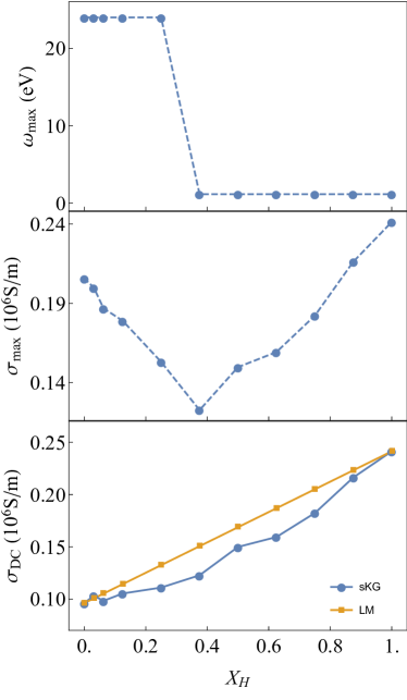
Figure 8: The maximal conductivity frequency $\omega_{max}$ (top panel), maximal conductivity $\sigma_{max}$ (middle panel) and the DC conductivity of the actual (round blue markers) and the linear-mixing model $\sigma_{\text{LM}}$ (square orange markers), as a function of the hydrogen ratio $X_{H}$ in He-H mixtures.

Finally, we compare the spectra in the different concentrations to a model of linear averaging of pure helium and pure hydrogen spectra, defined as

$$\sigma_{\text{LM}}\left(X_{\text{H}};\omega\right)=X_{\text{H}}\sigma\left(1;\omega\right)+\left(1-X_{\text{H}}\right)\sigma\left(0;\omega\right)\;.$$ (12)

It can be seen in the lower panel of Fig. 8 that the DC conductivity $\sigma_{LM}\left(X_{\text{H}};0\right)$ based on the linear averaging model is typically greater than the corresponding value calculated using sKG . This is due to the fact that in the actual system the environment each atom experiences includes, on the average, a mixture of He and H atoms while in the linear averaging model each atom is surrounded by atoms of its own kind.

IV Summary and Conclusions

In this work we presented a stochastic approach, sKG, to calculate the conductivity using Kubo-Greenwood formalism on top of a sDFT calculation. We showed that sKG conductivity can approach the values of the deterministic KS conductivity determined by the KG method when the number of sDFT-o’s and sKG-o’s are increased systematically. Moreover, the uniform sampling of all states of the system by sKG allows it to describe equally well the low-, mid- and high-end ranges of the spectrum, while the deterministic method is limited to lower energies due to memory and CPU constraints. The computational effort of the method scales linearly with system size and inversely proportional to the temperature similar to the sDFT calculations (Cytter et al., 2018) while the deterministic approach has cubic scaling both in system size and temperature.

As an application of the method, we studied the conductivity and DOS for mixed hydrogen and helium systems at a constant volume and temperature ($T=57\text{kK}$) ensemble. We found that the system displays two conductivity phases, where a transition from insulator to metal occurs at hydrogen atomic fraction of $X_{H}\approx 0.3$.

The method enlarges the scope of sDFT to study properties of warm dense matter for very large systems at high temperatures. This could be significant when large inhomogeneous systems are studied or in systems where the mixing occurs on the nanoscale.