Nonlinear Pose Filters on the Special Euclidean Group SE(3) with Guaranteed Transient and Steady-state Performance

Hashim A. Hashim, Lyndon J. Brown, and Kenneth McIsaac This work was supported in part by the NSERC Discovery Grant program.H. A. Hashim, L. J. Brown and K. McIsaac are with the Department of Electrical and Computer Engineering, University of Western Ontario, London, ON, Canada, N6A-5B9, e-mail: hmoham33@uwo.ca, lbrown@uwo.ca and kmcisaac@uwo.ca.
Abstract

Two novel nonlinear pose (i.e, attitude and position) filters developed directly on the Special Euclidean Group 𝕊𝔼(3)𝕊𝔼3\mathbb{SE}\left(3\right) able to guarantee prescribed characteristics of transient and steady-state performance are proposed. The position error and normalized Euclidean distance of attitude error are trapped to arbitrarily start within a given large set and converge systematically and asymptotically to the origin from almost any initial condition. The transient error is guaranteed not to exceed a prescribed value while the steady-state error is bounded by a predefined small value. The first pose filter operates based on a set of vectorial measurements coupled with a group of velocity vectors and requires preliminary pose reconstruction. The second filter, on the contrary, is able to perform its function using a set of vectorial measurements and a group of velocity vectors directly. Both proposed filters provide reasonable pose estimates with superior convergence properties while being able to use measurements obtained from low-cost inertial measurement, landmark measurement, and velocity measurement units. The equivalent quaternion representation and complete implementation steps of the proposed filters are presented. Simulation results demonstrate effectiveness and robustness of the proposed filters considering large error in initialization and high level of uncertainties in velocity vectors as well as in the set of vector measurements.

Index Terms:
Attitude, position, pose estimation, nonlinear observer, special orthogonal group, special Euclidean group, SO(3), SE(3), prescribed performance function, transient, steady-state error, transformed error, feature measurement, PPF, IMU.

I Introduction

Robotics and engineering applications such as aerial and underwater vehicles, satellites and space crafts are concerned with accurately estimating the pose of a rigid-body in 3D space. In essence, the pose of a rigid-body consists of two elements: orientation and position. The orientation of a rigid-body in 3D space is often referred to as attitude, therefore, orientation and attitude will be used interchangeably. One of the basic methods of attitude reconstruction is the algebraic approach. It allows to reconstruct the attitude given the availability of two or more non-collinear inertial-frame vectors and their body-frame vectors utilizing algorithms such as QUEST [1], or singular value decomposition (SVD) [2]. However, the process of attitude reconstruction is vulnerable to the effects of noise and bias contaminating the body-frame measurements which causes [1, 2] to produce unsatisfactory results. This is particularly true in the context of a rigid-body fitted with low-cost inertial measurement unit (IMU) [3, 4, 5].

Gaussian filters or nonlinear deterministic filters have been used historically to address the challenge of attitude estimation [3]. The family of Gaussian filters, which includes Kalman filter (KF) [6], extended KF (EKF) [7], and multiplicative EKF (MEKF) [8], often consider the unit quaternion in attitude representation [3, 5]. For good survey of Gaussian filters visit [3]. However, it is crucial to note the nonlinear nature of the attitude problem. Nonlinear attitude filters such as [3, 4, 9, 10, 11] are evolved directly on the Special Orthogonal Group 𝕊𝕆(3)𝕊𝕆3\mathbb{SO}\left(3\right). In particular, nonlinear deterministic attitude filters outperform the Gaussian filters in many respects, namely they are simpler in derivation and representation, they demand less processing power, and they show better tracking convergence [3, 4]. Attitude estimation is an essential part of the pose estimation problem. Taking into consideration the remarkable advantages of nonlinear attitude filters, attitude-position (pose) filtering problem is best approached in a nonlinear sense.

The pose estimation problem relies on filters evolved on the Special Euclidean Group 𝕊𝔼(3)𝕊𝔼3\mathbb{SE}\left(3\right) which require a measurement derived from a group velocity vector, vectorial measurements that could be provided by IMU, landmark measurements collected, for example, by a vision system and an estimate of the bias associated with velocity measurements. Pose estimation commonly involves a computer vision system with a monocular camera and IMU [12, 13, 14, 15]. The pose filter described in [13] was developed directly on 𝕊𝔼(3)𝕊𝔼3\mathbb{SE}\left(3\right) and its performance has been proven to be exponentially stable. Although, the filter in [13] requires pose reconstruction for the implementation, the nonlinear filter can be modified to function based solely on a set of vectorial measurements avoiding the need for pose reconstruction [16, 17]. In spite of the simplicity of the filter design in [13, 16, 17], numerical results show high sensitivity to noise and bias attached to the measurements. In addition, no systematic convergence is observed in [12, 13, 16, 17, 18, 19, 20, 14], such that the tracking error does not follow a predefined transient and steady-state measures. Accordingly, successful pose estimation for spacecraft control applications, such as [21, 22, 23, 24], cannot be achieved without pose filters which are robust against uncertain measurements, demonstrate fast tracking performance, and satisfy a certain level of transient and steady-state characteristics.

Prescribed performance implies confining the error to initially start within a predefined large set and decay systematically and smoothly to a predefined small residual set [25]. The error trajectory is constrained by a prescribed performance function (PPF) to satisfy transient as well as steady-state performance. The main objective of prescribed performance is to relax the constrained error to its unconstrained form, termed transformed error, which allows to keep the error within the decaying dynamic boundaries, and thereby achieve successful estimation or control applications. These applications include but are not limited to two degrees of freedom planar robots [25, 26], uncertain nonlinear systems [27], servo mechanism with friction compensation [28], and uncertain multi-agent system [29, 30].

In this paper two robust nonlinear pose filters on 𝕊𝔼(3)𝕊𝔼3\mathbb{SE}\left(3\right) with predefined transient as well as steady-state measures are proposed. The main contributions are as follows:

  1. 1)

    The proposed filters guarantee boundedness of the closed loop error signals with constrained error and unconstrained transformed error being proven to be almost globally asymptotically stable such that the error in the homogeneous transformation matrix is regulated asymptotically to the identity from almost any initial condition. Most significantly, the exceptional performance is guaranteed even when the measurements are supplied by a low-cost measurement unit, for instance, an IMU module equipped with a gyroscope, a vision unit, and a GPS.

  2. 2)

    The proposed filters guarantee systematic convergence of the error controlled by the dynamic reducing boundaries forcing the error to start within a predefined large set and decrease systematically and smoothly to a residual small set, unlike [12, 13, 16, 17, 18, 14].

  3. 3)

    The proposed pose filters are more efficient at ensuring fast convergence compared to similar estimators described in the literature, for instance [12, 13, 16, 17, 18, 14].

The fast convergence is mainly attributed to the dynamic behavior of the estimator gains. The first filter requires a group of velocity vectors and a set of measurements to obtain an online algebraic reconstruction of the pose. The second filter uses the group of velocity vector and the set of vectorial measurements directly.

The remainder of the paper is organized as follows: Section II gives an overview of 𝕊𝕆(3)𝕊𝕆3\mathbb{SO}\left(3\right) and 𝕊𝔼(3)𝕊𝔼3\mathbb{SE}\left(3\right), mathematical notation and identities. The pose problem is formulated, vector measurements are demonstrated and prescribed performance is introduced in Section III. The two proposed filters and the related stability analysis are presented in Section IV. Section V elaborates on the effectiveness and robustness of the proposed filters. Finally, Section VI draws a conclusion of this work.

II Preliminaries and Mathematical Identities

In this paper +subscript\mathbb{R}_{+} refers to the set of nonnegative real numbers. nsuperscript𝑛\mathbb{R}^{n} and n×msuperscript𝑛𝑚\mathbb{R}^{n\times m} denote a real n𝑛n-dimensional space column vector and real n×m𝑛𝑚n\times m dimensional space, respectively. The Euclidean norm of xn𝑥superscript𝑛x\in\mathbb{R}^{n} is x=xxnorm𝑥superscript𝑥top𝑥\left\|x\right\|=\sqrt{x^{\top}x} with being the transpose of the component. λ()𝜆\lambda\left(\cdot\right) denotes a set of singular values of a matrix with λ¯()¯𝜆\underline{\lambda}\left(\cdot\right) being its minimum value. 𝐈nsubscript𝐈𝑛\mathbf{I}_{n} stands for an n𝑛n-by-n𝑛n identity matrix, while 𝟎¯nnsubscript¯0𝑛superscript𝑛\underline{\mathbf{0}}_{n}\in\mathbb{R}^{n} is a zero column vector. The frame notation is as follows: {}\left\{\mathcal{B}\right\} refers to the body-frame and {}\left\{\mathcal{I}\right\} represents the inertial-frame.

Define 𝔾𝕃(3)𝔾𝕃3\mathbb{GL}\left(3\right) as a 3-dimensional general linear group which is a Lie group with smooth multiplication and inversion. The orthogonal group, denoted by 𝕆(3)𝕆3\mathbb{O}\left(3\right), is a subgroup of 𝔾𝕃(3)𝔾𝕃3\mathbb{GL}\left(3\right) defined by

𝕆(3)={M3×3|MM=MM=𝐈3}𝕆3conditional-set𝑀superscript33superscript𝑀top𝑀𝑀superscript𝑀topsubscript𝐈3\mathbb{O}\left(3\right)=\left\{\left.M\in\mathbb{R}^{3\times 3}\right|M^{\top}M=MM^{\top}=\mathbf{I}_{3}\right\}

with 𝐈3subscript𝐈3\mathbf{I}_{3} being a 3-by-3 identity matrix. Let 𝕊𝕆(3)𝕊𝕆3\mathbb{SO}\left(3\right) denote the Special Orthogonal Group which is a subgroup of 𝕆(3)𝕆3\mathbb{O}\left(3\right). The orientation of a rigid-body in 3D space is termed attitude, denoted by R𝑅R, and defined as follows:

𝕊𝕆(3)={R3×3|RR=RR=𝐈3det(R)=+1}𝕊𝕆3conditional-set𝑅superscript33𝑅superscript𝑅topsuperscript𝑅top𝑅subscript𝐈3det𝑅1\mathbb{SO}\left(3\right)=\left\{\left.R\in\mathbb{R}^{3\times 3}\right|RR^{\top}=R^{\top}R=\mathbf{I}_{3}\text{, }{\rm det}\left(R\right)=+1\right\}

with det()det{\rm det\left(\cdot\right)} being the determinant of the associated matrix. 𝕊𝔼(3)𝕊𝔼3\mathbb{SE}\left(3\right) stands for the Special Euclidean Group, a subset of the affine group 𝔾𝔸(3)=𝕊𝕆(3)×3𝔾𝔸3𝕊𝕆3superscript3\mathbb{GA}\left(3\right)=\mathbb{SO}\left(3\right)\times\mathbb{R}^{3} defined by

𝕊𝔼(3)={𝑻4×4|R𝕊𝕆(3),P3}𝕊𝔼3conditional-set𝑻superscript44formulae-sequence𝑅𝕊𝕆3𝑃superscript3\mathbb{SE}\left(3\right)=\left\{\left.\boldsymbol{T}\in\mathbb{R}^{4\times 4}\right|R\in\mathbb{SO}\left(3\right),P\in\mathbb{R}^{3}\right\}

where 𝑻𝕊𝔼(3)𝑻𝕊𝔼3\boldsymbol{T}\in\mathbb{SE}\left(3\right), termed a homogeneous transformation matrix, represents the pose of a rigid-body in 3D space with

𝑻=[RP𝟎¯31]𝕊𝔼(3)𝑻delimited-[]𝑅𝑃superscriptsubscript¯03top1𝕊𝔼3\boldsymbol{T}=\left[\begin{array}[]{cc}R&P\\ \underline{\mathbf{0}}_{3}^{\top}&1\end{array}\right]\in\mathbb{SE}\left(3\right) (1)

where P3𝑃superscript3P\in\mathbb{R}^{3} and R𝕊𝕆(3)𝑅𝕊𝕆3R\in\mathbb{SO}\left(3\right) denote position and attitude of a rigid-body in 3D space, respectively, and 𝟎¯3superscriptsubscript¯03top\underline{\mathbf{0}}_{3}^{\top} is a zero row. 𝔰𝔬(3)𝔰𝔬3\mathfrak{so}\left(3\right) is a Lie-algebra related to 𝕊𝕆(3)𝕊𝕆3\mathbb{SO}\left(3\right) defined by

𝔰𝔬(3)={A3×3|A=A}𝔰𝔬3conditional-set𝐴superscript33superscript𝐴top𝐴\mathfrak{so}\left(3\right)=\left\{\left.A\in\mathbb{R}^{3\times 3}\right|A^{\top}=-A\right\}

where A𝐴A is a skew symmetric matrix. Define the map []×:3𝔰𝔬(3):subscriptdelimited-[]superscript3𝔰𝔬3\left[\cdot\right]_{\times}:\mathbb{R}^{3}\rightarrow\mathfrak{so}\left(3\right) as

[α]×=[0α3α2α30α1α2α10]𝔰𝔬(3),α=[α1α2α3]formulae-sequencesubscriptdelimited-[]𝛼delimited-[]0subscript𝛼3subscript𝛼2subscript𝛼30subscript𝛼1subscript𝛼2subscript𝛼10𝔰𝔬3𝛼delimited-[]subscript𝛼1subscript𝛼2subscript𝛼3\left[\alpha\right]_{\times}=\left[\begin{array}[]{ccc}0&-\alpha_{3}&\alpha_{2}\\ \alpha_{3}&0&-\alpha_{1}\\ -\alpha_{2}&\alpha_{1}&0\end{array}\right]\in\mathfrak{so}\left(3\right),\hskip 10.00002pt\alpha=\left[\begin{array}[]{c}\alpha_{1}\\ \alpha_{2}\\ \alpha_{3}\end{array}\right]

For any α,β3𝛼𝛽superscript3\alpha,\beta\in\mathbb{R}^{3}, we define [α]×β=α×βsubscriptdelimited-[]𝛼𝛽𝛼𝛽\left[\alpha\right]_{\times}\beta=\alpha\times\beta with ×\times being the cross product. The wedge operator is denoted by \wedge, and for any 𝒴=[y1,y2]𝒴superscriptsuperscriptsubscript𝑦1topsuperscriptsubscript𝑦2toptop\mathcal{Y}=\left[y_{1}^{\top},y_{2}^{\top}\right]^{\top} with y1,y23subscript𝑦1subscript𝑦2superscript3y_{1},y_{2}\in\mathbb{R}^{3} the wedge map []:6𝔰𝔢(3):subscriptdelimited-[]superscript6𝔰𝔢3\left[\cdot\right]_{\wedge}:\mathbb{R}^{6}\rightarrow\mathfrak{se}\left(3\right) is defined by

[𝒴]=[[y1]×y2𝟎¯30]𝔰𝔢(3)subscriptdelimited-[]𝒴delimited-[]subscriptdelimited-[]subscript𝑦1subscript𝑦2superscriptsubscript¯03top0𝔰𝔢3\left[\mathcal{Y}\right]_{\wedge}=\left[\begin{array}[]{cc}\left[y_{1}\right]_{\times}&y_{2}\\ \underline{\mathbf{0}}_{3}^{\top}&0\end{array}\right]\in\mathfrak{se}\left(3\right)

𝔰𝔢(3)𝔰𝔢3\mathfrak{se}\left(3\right) is a Lie algebra of 𝕊𝔼(3)𝕊𝔼3\mathbb{SE}\left(3\right) and can be expressed as

𝔰𝔢(3)𝔰𝔢3\displaystyle\mathfrak{se}\left(3\right) ={[𝒴]4×4|y1,y23:[𝒴]=[[y1]×y20¯30]}absentconditional-setsubscriptdelimited-[]𝒴superscript44:subscript𝑦1subscript𝑦2superscript3subscriptdelimited-[]𝒴delimited-[]subscriptdelimited-[]subscript𝑦1subscript𝑦2superscriptsubscript¯03top0\displaystyle=\left\{\left.\left[\mathcal{Y}\right]_{\wedge}\in\mathbb{R}^{4\times 4}\right|\exists y_{1},y_{2}\in\mathbb{R}^{3}:\left[\mathcal{Y}\right]_{\wedge}=\left[\begin{array}[]{cc}\left[y_{1}\right]_{\times}&y_{2}\\ \underline{0}_{3}^{\top}&0\end{array}\right]\right\}

The inverse of []×subscriptdelimited-[]\left[\cdot\right]_{\times} is defined by 𝐯𝐞𝐱:𝔰𝔬(3)3:𝐯𝐞𝐱𝔰𝔬3superscript3\mathbf{vex}:\mathfrak{so}\left(3\right)\rightarrow\mathbb{R}^{3}, and for α3𝛼superscript3\alpha\in\mathbb{R}^{3} and [α]×𝔰𝔬(3)subscriptdelimited-[]𝛼𝔰𝔬3\left[\alpha\right]_{\times}\in\mathfrak{so}\left(3\right) we have

𝐯𝐞𝐱([α]×)=α3𝐯𝐞𝐱subscriptdelimited-[]𝛼𝛼superscript3\mathbf{vex}(\left[\alpha\right]_{\times})=\alpha\in\mathbb{R}^{3} (2)

𝓟asubscript𝓟𝑎\boldsymbol{\mathcal{P}}_{a} stands for an anti-symmetric projection operator on the Lie-algebra 𝔰𝔬(3)𝔰𝔬3\mathfrak{so}\left(3\right) while its mapping is given by 𝓟a:3×3𝔰𝔬(3):subscript𝓟𝑎superscript33𝔰𝔬3\boldsymbol{\mathcal{P}}_{a}:\mathbb{R}^{3\times 3}\rightarrow\mathfrak{so}\left(3\right) such that

𝓟a(M)=12(MM)𝔰𝔬(3),M3×3formulae-sequencesubscript𝓟𝑎𝑀12𝑀superscript𝑀top𝔰𝔬3𝑀superscript33\boldsymbol{\mathcal{P}}_{a}\left(M\right)=\frac{1}{2}(M-M^{\top})\in\mathfrak{so}\left(3\right),\,M\in\mathbb{R}^{3\times 3} (3)

The normalized Euclidean distance of the attitude matrix R𝕊𝕆(3)𝑅𝕊𝕆3R\in\mathbb{SO}\left(3\right) is given by

RI=14Tr{𝐈3R}subscriptnorm𝑅𝐼14Trsubscript𝐈3𝑅\left\|R\right\|_{I}=\frac{1}{4}{\rm Tr}\{\mathbf{I}_{3}-R\} (4)

with Tr{}Tr{\rm Tr}\left\{\cdot\right\} being a trace of a matrix, while RI[0,1]subscriptnorm𝑅𝐼01\left\|R\right\|_{I}\in\left[0,1\right]. To reconstruct the orientation of any rigid-body in 3D space it is sufficient to know unit-axis u3𝑢superscript3u\in\mathbb{R}^{3} in the sphere 𝕊2superscript𝕊2\mathbb{S}^{2} and angle of rotation α𝛼\alpha\in\mathbb{R} about u𝑢u. This type of parameterization is termed angle-axis parameterization and its mapping to 𝕊𝕆(3)𝕊𝕆3\mathbb{SO}\left(3\right) is given by α:×3𝕊𝕆(3):subscript𝛼superscript3𝕊𝕆3\mathcal{R}_{\alpha}:\mathbb{R}\times\mathbb{R}^{3}\rightarrow\mathbb{SO}\left(3\right) such that

α(α,u)=𝐈3+sin(α)[u]×+(1cos(α))[u]×2subscript𝛼𝛼𝑢subscript𝐈3𝛼subscriptdelimited-[]𝑢1𝛼superscriptsubscriptdelimited-[]𝑢2\mathcal{R}_{\alpha}(\alpha,u)=\mathbf{I}_{3}+\sin\left(\alpha\right)\left[u\right]_{\times}+\left(1-\cos\left(\alpha\right)\right)\left[u\right]_{\times}^{2} (5)

For α,β3𝛼𝛽superscript3\alpha,\beta\in{\rm\mathbb{R}}^{3}, R𝕊𝕆(3)𝑅𝕊𝕆3R\in\mathbb{SO}\left(3\right), A3×3𝐴superscript33A\in\mathbb{R}^{3\times 3} and B=B3×3𝐵superscript𝐵topsuperscript33B=B^{\top}\in\mathbb{R}^{3\times 3} the following mathematical identities

[α×β]×=subscriptdelimited-[]𝛼𝛽absent\displaystyle\left[\alpha\times\beta\right]_{\times}= βααβ𝛽superscript𝛼top𝛼superscript𝛽top\displaystyle\beta\alpha^{\top}-\alpha\beta^{\top} (6)
[Rα]×=subscriptdelimited-[]𝑅𝛼absent\displaystyle\left[R\alpha\right]_{\times}= R[α]×R𝑅subscriptdelimited-[]𝛼superscript𝑅top\displaystyle R\left[\alpha\right]_{\times}R^{\top} (7)
[α]×2=superscriptsubscriptdelimited-[]𝛼2absent\displaystyle\left[\alpha\right]_{\times}^{2}= αα𝐈3+ααsuperscript𝛼top𝛼subscript𝐈3𝛼superscript𝛼top\displaystyle-\alpha^{\top}\alpha\mathbf{I}_{3}+\alpha\alpha^{\top} (8)
B[α]×+[α]×B=𝐵subscriptdelimited-[]𝛼subscriptdelimited-[]𝛼𝐵absent\displaystyle B\left[\alpha\right]_{\times}+\left[\alpha\right]_{\times}B= Tr{B}[α]×[Bα]×Tr𝐵subscriptdelimited-[]𝛼subscriptdelimited-[]𝐵𝛼\displaystyle{\rm Tr}\left\{B\right\}\left[\alpha\right]_{\times}-\left[B\alpha\right]_{\times} (9)
Tr{B[α]×}=Tr𝐵subscriptdelimited-[]𝛼absent\displaystyle{\rm Tr}\{B\left[\alpha\right]_{\times}\}= 00\displaystyle 0 (10)
Tr{A[α]×}=Tr𝐴subscriptdelimited-[]𝛼absent\displaystyle{\rm Tr}\{A\left[\alpha\right]_{\times}\}= Tr{𝓟a(A)[α]×}=2𝐯𝐞𝐱(𝓟a(A))αTrsubscript𝓟𝑎𝐴subscriptdelimited-[]𝛼2𝐯𝐞𝐱superscriptsubscript𝓟𝑎𝐴top𝛼\displaystyle{\rm Tr}\{\boldsymbol{\mathcal{P}}_{a}\left(A\right)\left[\alpha\right]_{\times}\}=-2\mathbf{vex}(\boldsymbol{\mathcal{P}}_{a}(A))^{\top}\alpha (11)

will be used in the subsequent derivations.

III Problem Formulation with Prescribed Performance

Pose estimator relies on a set of vectorial measurements made on inertial-frame and body-frame. This section aims to define the pose problem and present the associated measurements. Next, the pose error and its reformulation are geared towards attaining desired characteristics of transient and steady-state performance.

III-A Pose Kinematics and Measurements

The pose of any rigid-body in 3D space consists of two elements: attitude and position, and this work aims to estimate both elements. The attitude of a rigid-body is commonly represented by a rotational matrix R𝕊𝕆(3)𝑅𝕊𝕆3R\in\mathbb{SO}\left(3\right) defined relative to the body-frame such that R{}𝑅R\in\left\{\mathcal{B}\right\}. Position of a rigid-body is, on the contrary, defined by P3𝑃superscript3P\in\mathbb{R}^{3} with respect to the inertial-frame P{}𝑃P\in\left\{\mathcal{I}\right\}. The pose problem can be characterized by the homogeneous transformation matrix 𝑻𝕊𝔼(3)𝑻𝕊𝔼3\boldsymbol{T}\in\mathbb{SE}\left(3\right) as

𝑻=[RP𝟎¯31]𝑻delimited-[]𝑅𝑃superscriptsubscript¯03top1\boldsymbol{T}=\left[\begin{array}[]{cc}R&P\\ \underline{\mathbf{0}}_{3}^{\top}&1\end{array}\right] (12)

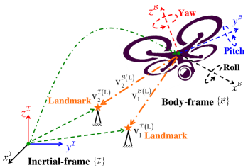
The pose estimation problem of a rigid-body in 3D space is depicted in Fig. 1.
Refer to caption
Figure 1: Pose estimation problem of a rigid-body in 3D space.

Let the components associated with body-frame and inertial-frame be assigned superscripts \mathcal{B} and \mathcal{I}, respectively. The attitude can be obtained given NRsubscript𝑁RN_{{\rm R}} known non-collinear inertial vectors, available for measurements at a coordinate fixed to the moving body. IMU exemplify sensors, which could provide those measurements. The i𝑖ith body-frame vector measurement is given by

[vi(R)0]=𝑻1[vi(R)0]+[bi(R)0]+[ωi(R)0]delimited-[]superscriptsubscriptv𝑖R0superscript𝑻1delimited-[]superscriptsubscriptv𝑖R0delimited-[]superscriptsubscriptb𝑖R0delimited-[]superscriptsubscript𝜔𝑖R0\left[\begin{array}[]{c}{\rm v}_{i}^{\mathcal{B}\left({\rm R}\right)}\\ 0\end{array}\right]=\boldsymbol{T}^{-1}\left[\begin{array}[]{c}{\rm v}_{i}^{\mathcal{I}\left({\rm R}\right)}\\ 0\end{array}\right]+\left[\begin{array}[]{c}{\rm b}_{i}^{\mathcal{B}\left({\rm R}\right)}\\ 0\end{array}\right]+\left[\begin{array}[]{c}\omega_{i}^{\mathcal{B}\left({\rm R}\right)}\\ 0\end{array}\right]

such that

vi(R)=Rvi(R)+bi(R)+ωi(R)superscriptsubscriptv𝑖Rsuperscript𝑅topsuperscriptsubscriptv𝑖Rsuperscriptsubscriptb𝑖Rsuperscriptsubscript𝜔𝑖R{\rm v}_{i}^{\mathcal{B}\left({\rm R}\right)}=R^{\top}{\rm v}_{i}^{\mathcal{I}\left({\rm R}\right)}+{\rm b}_{i}^{\mathcal{B}\left({\rm R}\right)}+\omega_{i}^{\mathcal{B}\left({\rm R}\right)} (13)

with vi(R)superscriptsubscriptv𝑖R{\rm v}_{i}^{\mathcal{I}\left({\rm R}\right)} being the i𝑖ith known vector in the inertial-frame, and bi(R)superscriptsubscriptb𝑖R{\rm b}_{i}^{\mathcal{B}\left({\rm R}\right)} and ωi(R)superscriptsubscript𝜔𝑖R\omega_{i}^{\mathcal{B}\left({\rm R}\right)} being unknown bias and noise components added to the i𝑖ith measurement, respectively, for all vi(R),vi(R),bi(R),ωi(R)3superscriptsubscriptv𝑖Rsuperscriptsubscriptv𝑖Rsuperscriptsubscriptb𝑖Rsuperscriptsubscript𝜔𝑖Rsuperscript3{\rm v}_{i}^{\mathcal{B}\left({\rm R}\right)},{\rm v}_{i}^{\mathcal{I}\left({\rm R}\right)},{\rm b}_{i}^{\mathcal{B}\left({\rm R}\right)},\omega_{i}^{\mathcal{B}\left({\rm R}\right)}\in\mathbb{R}^{3} and i=1,2,,NR𝑖12subscript𝑁Ri=1,2,\ldots,N_{{\rm R}}. The known inertial vector vi(R)superscriptsubscriptv𝑖R{\rm v}_{i}^{\mathcal{I}\left({\rm R}\right)} and the available body-frame measurement vi(R)superscriptsubscriptv𝑖R{\rm v}_{i}^{\mathcal{B}\left({\rm R}\right)} in (13) can be normalized such that

υi(R)=vi(R)vi(R),υi(R)=vi(R)vi(R)formulae-sequencesuperscriptsubscript𝜐𝑖Rsuperscriptsubscriptv𝑖Rnormsuperscriptsubscriptv𝑖Rsuperscriptsubscript𝜐𝑖Rsuperscriptsubscriptv𝑖Rnormsuperscriptsubscriptv𝑖R\upsilon_{i}^{\mathcal{I}\left({\rm R}\right)}=\frac{{\rm v}_{i}^{\mathcal{I}\left({\rm R}\right)}}{\left\|{\rm v}_{i}^{\mathcal{I}\left({\rm R}\right)}\right\|},\hskip 10.00002pt\upsilon_{i}^{\mathcal{B}\left({\rm R}\right)}=\frac{{\rm v}_{i}^{\mathcal{B}\left({\rm R}\right)}}{\left\|{\rm v}_{i}^{\mathcal{B}\left({\rm R}\right)}\right\|} (14)

Thus, the attitude of a rigid-body can be extracted using υi(R)superscriptsubscript𝜐𝑖R\upsilon_{i}^{\mathcal{I}\left({\rm R}\right)} and υi(R)superscriptsubscript𝜐𝑖R\upsilon_{i}^{\mathcal{B}\left({\rm R}\right)} in (14) rather than vi(R)superscriptsubscriptv𝑖R{\rm v}_{i}^{\mathcal{I}\left({\rm R}\right)} and vi(R)superscriptsubscriptv𝑖R{\rm v}_{i}^{\mathcal{B}\left({\rm R}\right)}. Let us introduce the following two sets

υ(R)superscript𝜐R\displaystyle\upsilon^{\mathcal{I}\left({\rm R}\right)} =[υ1(R),,υNR(R)]{}absentsuperscriptsubscript𝜐1Rsuperscriptsubscript𝜐subscript𝑁RR\displaystyle=\left[\upsilon_{1}^{\mathcal{I}\left({\rm R}\right)},\ldots,\upsilon_{N_{{\rm R}}}^{\mathcal{I}\left({\rm R}\right)}\right]\in\left\{\mathcal{I}\right\}
υ(R)superscript𝜐R\displaystyle\upsilon^{\mathcal{B}\left({\rm R}\right)} =[υ1(R),,υNR(R)]{}absentsuperscriptsubscript𝜐1Rsuperscriptsubscript𝜐subscript𝑁RR\displaystyle=\left[\upsilon_{1}^{\mathcal{B}\left({\rm R}\right)},\ldots,\upsilon_{N_{{\rm R}}}^{\mathcal{B}\left({\rm R}\right)}\right]\in\left\{\mathcal{B}\right\} (15)

where the two sets in (15) include the normalized vectors in (14) for all υ(R),υ(R)3×NRsuperscript𝜐Rsuperscript𝜐Rsuperscript3subscript𝑁R\upsilon^{\mathcal{I}\left({\rm R}\right)},\upsilon^{\mathcal{B}\left({\rm R}\right)}\in\mathbb{R}^{3\times N_{{\rm R}}}. The position of the moving body can be extracted if its attitude R𝑅R has already been determined and there exist NLsubscript𝑁LN_{{\rm L}} known landmarks (feature points) obtained, for example, by a vision system. The i𝑖ith body-frame landmark measurement is given by

[vi(L)1]=𝑻1[vi(L)1]+[bi(L)0]+[ωi(L)0]delimited-[]superscriptsubscriptv𝑖L1superscript𝑻1delimited-[]superscriptsubscriptv𝑖L1delimited-[]superscriptsubscriptb𝑖L0delimited-[]superscriptsubscript𝜔𝑖L0\left[\begin{array}[]{c}{\rm v}_{i}^{\mathcal{B}\left({\rm L}\right)}\\ 1\end{array}\right]=\boldsymbol{T}^{-1}\left[\begin{array}[]{c}{\rm v}_{i}^{\mathcal{I}\left({\rm L}\right)}\\ 1\end{array}\right]+\left[\begin{array}[]{c}{\rm b}_{i}^{\mathcal{B}\left({\rm L}\right)}\\ 0\end{array}\right]+\left[\begin{array}[]{c}\omega_{i}^{\mathcal{B}\left({\rm L}\right)}\\ 0\end{array}\right]

such that

vi(L)=R(vi(L)P)+bi(L)+ωi(L)superscriptsubscriptv𝑖Lsuperscript𝑅topsuperscriptsubscriptv𝑖L𝑃superscriptsubscriptb𝑖Lsuperscriptsubscript𝜔𝑖L{\rm v}_{i}^{\mathcal{B}\left({\rm L}\right)}=R^{\top}\left({\rm v}_{i}^{\mathcal{I}\left({\rm L}\right)}-P\right)+{\rm b}_{i}^{\mathcal{B}\left({\rm L}\right)}+\omega_{i}^{\mathcal{B}\left({\rm L}\right)} (16)

where vi(L)superscriptsubscriptv𝑖L{\rm v}_{i}^{\mathcal{I}\left({\rm L}\right)} is the i𝑖ith known fixed landmark located in the inertial-frame, bi(L)superscriptsubscriptb𝑖L{\rm b}_{i}^{\mathcal{B}\left({\rm L}\right)} and ωi(L)superscriptsubscript𝜔𝑖L\omega_{i}^{\mathcal{B}\left({\rm L}\right)} are the additive unknown bias and noise vectors of the i𝑖ith measurement, respectively, for all vi(L),vi(L),bi(L),ωi(L)3superscriptsubscriptv𝑖Lsuperscriptsubscriptv𝑖Lsuperscriptsubscriptb𝑖Lsuperscriptsubscript𝜔𝑖Lsuperscript3{\rm v}_{i}^{\mathcal{B}\left({\rm L}\right)},{\rm v}_{i}^{\mathcal{I}\left({\rm L}\right)},{\rm b}_{i}^{\mathcal{B}\left({\rm L}\right)},\omega_{i}^{\mathcal{B}\left({\rm L}\right)}\in\mathbb{R}^{3} and i=1,2,,NL𝑖12subscript𝑁Li=1,2,\ldots,N_{{\rm L}}. Define the set of inertial-frame and body-frame vectors associated with landmarks by

v(L)superscriptvL\displaystyle{\rm v}^{\mathcal{B}\left({\rm L}\right)} =[v1(L),,vNL(L)]{}absentsuperscriptsubscriptv1Lsuperscriptsubscriptvsubscript𝑁LL\displaystyle=\left[{\rm v}_{1}^{\mathcal{B}\left({\rm L}\right)},\ldots,{\rm v}_{N_{{\rm L}}}^{\mathcal{B}\left({\rm L}\right)}\right]\in\left\{\mathcal{B}\right\}
v(L)superscriptvL\displaystyle{\rm v}^{\mathcal{I}\left({\rm L}\right)} =[v1(L),,vNL(L)]{}absentsuperscriptsubscriptv1Lsuperscriptsubscriptvsubscript𝑁LL\displaystyle=\left[{\rm v}_{1}^{\mathcal{I}\left({\rm L}\right)},\ldots,{\rm v}_{N_{{\rm L}}}^{\mathcal{I}\left({\rm L}\right)}\right]\in\left\{\mathcal{I}\right\} (17)

In case when more than one landmark is available for measurement, it is common to obtain a weighted geometric center of all the landmarks, which can be calculated as follows:

𝒢csuperscriptsubscript𝒢𝑐\displaystyle\mathcal{G}_{c}^{\mathcal{I}} =1i=1NLkiLi=1NLkiLvi(L)absent1superscriptsubscript𝑖1subscript𝑁Lsuperscriptsubscript𝑘𝑖Lsuperscriptsubscript𝑖1subscript𝑁Lsuperscriptsubscript𝑘𝑖Lsuperscriptsubscriptv𝑖L\displaystyle=\frac{1}{\sum_{i=1}^{N_{{\rm L}}}k_{i}^{{\rm L}}}\sum_{i=1}^{N_{{\rm L}}}k_{i}^{{\rm L}}{\rm v}_{i}^{\mathcal{I}\left({\rm L}\right)} (18)
𝒢csuperscriptsubscript𝒢𝑐\displaystyle\mathcal{G}_{c}^{\mathcal{B}} =1i=1NLkiLi=1NLkiLvi(L)absent1superscriptsubscript𝑖1subscript𝑁Lsuperscriptsubscript𝑘𝑖Lsuperscriptsubscript𝑖1subscript𝑁Lsuperscriptsubscript𝑘𝑖Lsuperscriptsubscriptv𝑖L\displaystyle=\frac{1}{\sum_{i=1}^{N_{{\rm L}}}k_{i}^{{\rm L}}}\sum_{i=1}^{N_{{\rm L}}}k_{i}^{{\rm L}}{\rm v}_{i}^{\mathcal{B}\left({\rm L}\right)} (19)

such that kiLsuperscriptsubscript𝑘𝑖Lk_{i}^{{\rm L}} is the confidence level of the i𝑖ith measurement.

Assumption 1.

(Rigid-body pose observability) The pose of a rigid-body in 3D space can be extracted given the availability of at least two non-collinear vectors from the sets in (15) (NR2subscript𝑁R2N_{{\rm R}}\geq 2) and at least one feature point from the sets in (17) with NL1subscript𝑁L1N_{{\rm L}}\geq 1. In the case when NR=2subscript𝑁R2N_{{\rm R}}=2, the third vector can be obtained by the means of cross multiplication: υ3(R)=υ1(R)×υ2(R)superscriptsubscript𝜐3Rsuperscriptsubscript𝜐1Rsuperscriptsubscript𝜐2R\upsilon_{3}^{\mathcal{I}\left({\rm R}\right)}=\upsilon_{1}^{\mathcal{I}\left({\rm R}\right)}\times\upsilon_{2}^{\mathcal{I}\left({\rm R}\right)} and υ3(R)=υ1(R)×υ2(R)superscriptsubscript𝜐3Rsuperscriptsubscript𝜐1Rsuperscriptsubscript𝜐2R\upsilon_{3}^{\mathcal{B}\left({\rm R}\right)}=\upsilon_{1}^{\mathcal{B}\left({\rm R}\right)}\times\upsilon_{2}^{\mathcal{B}\left({\rm R}\right)}.

According to Assumption 1 a set of vectorial measurement described in (15) is sufficient to have rank 3. Accordingly, the homogeneous transformation matrix 𝑻𝑻\boldsymbol{T} can be extracted if Assumption 1 is met. For simplicity, the body-frame vectors vi(R)superscriptsubscriptv𝑖R{\rm v}_{i}^{\mathcal{B}\left({\rm R}\right)} and vi(L)superscriptsubscriptv𝑖L{\rm v}_{i}^{\mathcal{B}\left({\rm L}\right)} are considered to be noise and bias free in the stability analysis. In the Simulation Section, on the contrary, the noise and bias corrupting the measurements of vi(R)superscriptsubscriptv𝑖R{\rm v}_{i}^{\mathcal{B}\left({\rm R}\right)} and vi(L)superscriptsubscriptv𝑖L{\rm v}_{i}^{\mathcal{B}\left({\rm L}\right)} are taken into consideration. The pose kinematics of the homogeneous transformation matrix 𝑻𝑻\boldsymbol{T} in (12) are given by

[R˙P˙𝟎¯30]=[RP𝟎¯31][[Ω]×V𝟎¯30]delimited-[]˙𝑅˙𝑃superscriptsubscript¯03top0delimited-[]𝑅𝑃superscriptsubscript¯03top1delimited-[]subscriptdelimited-[]Ω𝑉superscriptsubscript¯03top0\left[\begin{array}[]{cc}\dot{R}&\dot{P}\\ \underline{\mathbf{0}}_{3}^{\top}&0\end{array}\right]=\left[\begin{array}[]{cc}R&P\\ \underline{\mathbf{0}}_{3}^{\top}&1\end{array}\right]\left[\begin{array}[]{cc}\left[\Omega\right]_{\times}&V\\ \underline{\mathbf{0}}_{3}^{\top}&0\end{array}\right]

such that

P˙˙𝑃\displaystyle\dot{P} =RVabsent𝑅𝑉\displaystyle=RV
R˙˙𝑅\displaystyle\dot{R} =R[Ω]×absent𝑅subscriptdelimited-[]Ω\displaystyle=R\left[\Omega\right]_{\times} (20)
𝑻˙˙𝑻\displaystyle\dot{\boldsymbol{T}} =𝑻[𝒴]absent𝑻subscriptdelimited-[]𝒴\displaystyle=\boldsymbol{T}\left[\mathcal{Y}\right]_{\wedge} (21)

with Ω3Ωsuperscript3\Omega\in\mathbb{R}^{3} and V3𝑉superscript3V\in\mathbb{R}^{3} being the true angular and translational velocity of the moving body, respectively, and 𝒴=[Ω,V]6𝒴superscriptsuperscriptΩtopsuperscript𝑉toptopsuperscript6\mathcal{Y}=\left[\Omega^{\top},V^{\top}\right]^{\top}\in\mathbb{R}^{6} being the group velocity vector. The angular velocity can be measured by a gyroscope, for example, and expressed as follows:

Ωm=Ω+bΩ+ωΩ{}subscriptΩ𝑚Ωsubscript𝑏Ωsubscript𝜔Ω\Omega_{m}=\Omega+b_{\Omega}+\omega_{\Omega}\in\left\{\mathcal{B}\right\} (22)

where bΩsubscript𝑏Ωb_{\Omega} is an unknown constant or slowly time-varying bias, and ωΩsubscript𝜔Ω\omega_{\Omega} is an unknown random noise attached to the measurement, for all bΩ,ωΩ3subscript𝑏Ωsubscript𝜔Ωsuperscript3b_{\Omega},\omega_{\Omega}\in\mathbb{R}^{3}. Likewise, the translational velocity measurement of a moving body can be obtained using a GPS, for instance, and defined by

Vm=V+bV+ωV{}subscript𝑉𝑚𝑉subscript𝑏𝑉subscript𝜔𝑉V_{m}=V+b_{V}+\omega_{V}\in\left\{\mathcal{B}\right\} (23)

with bV3subscript𝑏𝑉superscript3b_{V}\in\mathbb{R}^{3} denoting an unknown constant or slowly time-varying bias, and ωV3subscript𝜔𝑉superscript3\omega_{V}\in\mathbb{R}^{3} being random noise attached to the translational velocity measurements. The group of velocity measurements and bias associated with it can be defined by 𝒴m=[Ωm,Vm]6subscript𝒴𝑚superscriptsuperscriptsubscriptΩ𝑚topsuperscriptsubscript𝑉𝑚toptopsuperscript6\mathcal{Y}_{m}=\left[\Omega_{m}^{\top},V_{m}^{\top}\right]^{\top}\in\mathbb{R}^{6} and b=[bΩ,bV]6𝑏superscriptsuperscriptsubscript𝑏Ωtopsuperscriptsubscript𝑏𝑉toptopsuperscript6b=\left[b_{\Omega}^{\top},b_{V}^{\top}\right]^{\top}\in\mathbb{R}^{6}, respectively. For the sake of simplicity, we consider ωΩ=ωV=𝟎¯3subscript𝜔Ωsubscript𝜔𝑉subscript¯03\omega_{\Omega}=\omega_{V}=\underline{\mathbf{0}}_{3} in the analysis. However, in the implementation it is used ωΩ𝟎¯3subscript𝜔Ωsubscript¯03\omega_{\Omega}\neq\underline{\mathbf{0}}_{3} and ωV𝟎¯3subscript𝜔𝑉subscript¯03\omega_{V}\neq\underline{\mathbf{0}}_{3}. Considering the normalized Euclidean distance of the rotational matrix R𝑅R in (4) and the identity in (11), the true attitude kinematics in (20) can be expressed in view of (4) as

R˙Isubscriptnorm˙𝑅𝐼\displaystyle||\dot{R}||_{I} =14Tr{R˙}absent14Tr˙𝑅\displaystyle=-\frac{1}{4}{\rm Tr}\{\dot{R}\}
=14Tr{𝓟a(R)[Ω]×}absent14Trsubscript𝓟𝑎𝑅subscriptdelimited-[]Ω\displaystyle=-\frac{1}{4}{\rm Tr}\{\boldsymbol{\mathcal{P}}_{a}\left(R\right)\left[\Omega\right]_{\times}\}
=12𝐯𝐞𝐱(𝓟a(R))Ωabsent12𝐯𝐞𝐱superscriptsubscript𝓟𝑎𝑅topΩ\displaystyle=\frac{1}{2}\mathbf{vex}(\boldsymbol{\mathcal{P}}_{a}(R))^{\top}\Omega (24)

Accordingly, the problem of pose kinematics in (21) can be reformulated and expressed in vector form as

[R˙IP˙]=[12𝐯𝐞𝐱(𝓟a(R))𝟎¯3𝟎3×3R][ΩmbΩVmbV]delimited-[]subscriptnorm˙𝑅𝐼˙𝑃delimited-[]12𝐯𝐞𝐱superscriptsubscript𝓟𝑎𝑅topsuperscriptsubscript¯03topsubscript033𝑅delimited-[]subscriptΩ𝑚subscript𝑏Ωsubscript𝑉𝑚subscript𝑏𝑉\left[\begin{array}[]{c}||\dot{R}||_{I}\\ \dot{P}\end{array}\right]=\left[\begin{array}[]{cc}\frac{1}{2}\mathbf{vex}(\boldsymbol{\mathcal{P}}_{a}(R))^{\top}&\underline{\mathbf{0}}_{3}^{\top}\\ \mathbf{0}_{3\times 3}&R\end{array}\right]\left[\begin{array}[]{c}\Omega_{m}-b_{\Omega}\\ V_{m}-b_{V}\end{array}\right] (25)

with 𝟎3×3subscript033\mathbf{0}_{3\times 3} being a zero matrix and ωΩ=ωV=𝟎¯3subscript𝜔Ωsubscript𝜔𝑉subscript¯03\omega_{\Omega}=\omega_{V}=\underline{\mathbf{0}}_{3}. Let the estimate of the homogeneous transformation matrix in (12), denoted by 𝑻^^𝑻\hat{\boldsymbol{T}}, be given by

𝑻^=[R^P^𝟎¯31]^𝑻delimited-[]^𝑅^𝑃superscriptsubscript¯03top1\hat{\boldsymbol{T}}=\left[\begin{array}[]{cc}\hat{R}&\hat{P}\\ \underline{\mathbf{0}}_{3}^{\top}&1\end{array}\right] (26)

with R^^𝑅\hat{R} and P^^𝑃\hat{P} being the estimates of R𝑅R and P𝑃P, respectively. Let us define the error in the homogeneous transformation matrix from body-frame to estimator-frame by

𝑻~~𝑻\displaystyle\tilde{\boldsymbol{T}} =𝑻^𝑻1=[R~P^R~P𝟎¯31]=[R~P~𝟎¯31]absent^𝑻superscript𝑻1delimited-[]~𝑅^𝑃~𝑅𝑃superscriptsubscript¯03top1delimited-[]~𝑅~𝑃superscriptsubscript¯03top1\displaystyle=\hat{\boldsymbol{T}}\boldsymbol{T}^{-1}=\left[\begin{array}[]{cc}\tilde{R}&\hat{P}-\tilde{R}P\\ \underline{\mathbf{0}}_{3}^{\top}&1\end{array}\right]=\left[\begin{array}[]{cc}\tilde{R}&\tilde{P}\\ \underline{\mathbf{0}}_{3}^{\top}&1\end{array}\right] (31)

where R~=R^R~𝑅^𝑅superscript𝑅top\tilde{R}=\hat{R}R^{\top} and P~~𝑃\tilde{P} are the errors associated with attitude and position, respectively. The aim of this work is to drive 𝑻^𝑻^𝑻𝑻\hat{\boldsymbol{T}}\rightarrow\boldsymbol{T} which in turn guarantees driving P~𝟎¯3~𝑃subscript¯03\tilde{P}\rightarrow\underline{\mathbf{0}}_{3}, R~𝐈3~𝑅subscript𝐈3\tilde{R}\rightarrow\mathbf{I}_{3}, and 𝑻~𝐈4~𝑻subscript𝐈4\tilde{\boldsymbol{T}}\rightarrow\mathbf{I}_{4}. Lemma 1 presented below will prove useful in the subsequent filter derivation.

Lemma 1.

Let R𝕊𝕆(3)𝑅𝕊𝕆3R\in\mathbb{SO}\left(3\right), M=M3×3𝑀superscript𝑀topsuperscript33M=M^{\top}\in\mathbb{R}^{3\times 3}, M𝑀M have rank 3, Tr{M}=3Tr𝑀3{\rm Tr}\left\{M\right\}=3, and 𝐌¯=Tr{M}𝐈3M¯𝐌Tr𝑀subscript𝐈3𝑀\bar{\mathbf{M}}={\rm Tr}\left\{M\right\}\mathbf{I}_{3}-M, while the minimum singular value of 𝐌¯¯𝐌\bar{\mathbf{M}} is λ¯:=λ¯(𝐌¯)assign¯𝜆¯𝜆¯𝐌\underline{\lambda}:=\underline{\lambda}(\bar{\mathbf{M}}). Then, the following holds:

𝐯𝐞𝐱(𝓟a(R))2superscriptnorm𝐯𝐞𝐱subscript𝓟𝑎𝑅2\displaystyle||\mathbf{vex}(\boldsymbol{\mathcal{P}}_{a}(R))||^{2} =4(1RI)RIabsent41subscriptnorm𝑅𝐼subscriptnorm𝑅𝐼\displaystyle=4(1-||R||_{I})||R||_{I} (32)
2λ¯𝐯𝐞𝐱(𝓟a(RM))21+Tr{RMM1}2¯𝜆superscriptnorm𝐯𝐞𝐱subscript𝓟𝑎𝑅𝑀21Tr𝑅𝑀superscript𝑀1\displaystyle\frac{2}{\underline{\lambda}}\frac{||\mathbf{vex}(\boldsymbol{\mathcal{P}}_{a}(RM))||^{2}}{1+{\rm Tr}\{RMM^{-1}\}} RMIabsentsubscriptnorm𝑅𝑀𝐼\displaystyle\geq\left\|RM\right\|_{I} (33)

Proof. See Appendix A.

III-B Prescribed Performance

Considering the error in the homogeneous transformation matrix as in (31) and in view of the pose kinematics in (25), let us define the error in vector form by

𝒆=[𝒆1,𝒆2,𝒆3,𝒆4]=[R~I,P~]4𝒆superscriptsubscript𝒆1subscript𝒆2subscript𝒆3subscript𝒆4topsuperscriptsubscriptnorm~𝑅𝐼superscript~𝑃toptopsuperscript4\boldsymbol{e}=\left[\boldsymbol{e}_{1},\boldsymbol{e}_{2},\boldsymbol{e}_{3},\boldsymbol{e}_{4}\right]^{\top}=\left[||\tilde{R}||_{I},\tilde{P}^{\top}\right]^{\top}\in\mathbb{R}^{4} (34)

The objective of this subsection is to reformulate the problem such that the error in (34) satisfies transient as well as steady-state measures predefined by the user. This can be achieved by guiding the error vector 𝒆𝒆\boldsymbol{e} to initiate within a large known set and after decaying smoothly and systematically settle within a predefined small set using prescribed performance function (PPF) [25, 29]. The PPF is defined by ξi(t)subscript𝜉𝑖𝑡\xi_{i}\left(t\right) which is a positive smooth time-decreasing function which satisfies ξi:++:subscript𝜉𝑖subscriptsubscript\xi_{i}:\mathbb{R}_{+}\to\mathbb{R}_{+} and limtξi(t)=ξi>0subscript𝑡subscript𝜉𝑖𝑡superscriptsubscript𝜉𝑖0\lim\limits_{t\to\infty}\xi_{i}\left(t\right)=\xi_{i}^{\infty}>0 and can be expressed by [25]

ξi(t)=(ξi0ξi)exp(it)+ξisubscript𝜉𝑖𝑡superscriptsubscript𝜉𝑖0superscriptsubscript𝜉𝑖subscript𝑖𝑡superscriptsubscript𝜉𝑖\xi_{i}\left(t\right)=\left(\xi_{i}^{0}-\xi_{i}^{\infty}\right)\exp\left(-\ell_{i}t\right)+\xi_{i}^{\infty} (35)

with ξi(0)=ξi0subscript𝜉𝑖0superscriptsubscript𝜉𝑖0\xi_{i}\left(0\right)=\xi_{i}^{0} being the initial value of the PPF and the upper bound of the known large set, ξisuperscriptsubscript𝜉𝑖\xi_{i}^{\infty} being the upper bound of the narrow set, and isubscript𝑖\ell_{i} being a positive constant controlling the convergence rate of ξ(t)𝜉𝑡\xi\left(t\right) from ξi0superscriptsubscript𝜉𝑖0\xi_{i}^{0} to ξisuperscriptsubscript𝜉𝑖\xi_{i}^{\infty} for all i=1,,4𝑖14i=1,\ldots,4. The error 𝒆i(t)subscript𝒆𝑖𝑡\boldsymbol{e}_{i}\left(t\right) is guaranteed to follow the predefined transient and steady-state boundaries, if the conditions below are met:

δξi(t)<𝒆i(t)<ξi(t),𝛿subscript𝜉𝑖𝑡subscript𝒆𝑖𝑡subscript𝜉𝑖𝑡\displaystyle-\delta\xi_{i}\left(t\right)<\boldsymbol{e}_{i}\left(t\right)<\xi_{i}\left(t\right), if 𝒆i(0)>0if subscript𝒆𝑖00\displaystyle\text{ if }\boldsymbol{e}_{i}\left(0\right)>0 (36)
ξi(t)<𝒆i(t)<δξi(t),subscript𝜉𝑖𝑡subscript𝒆𝑖𝑡𝛿subscript𝜉𝑖𝑡\displaystyle-\xi_{i}\left(t\right)<\boldsymbol{e}_{i}\left(t\right)<\delta\xi_{i}\left(t\right), if 𝒆i(0)<0if subscript𝒆𝑖00\displaystyle\text{ if }\boldsymbol{e}_{i}\left(0\right)<0 (37)

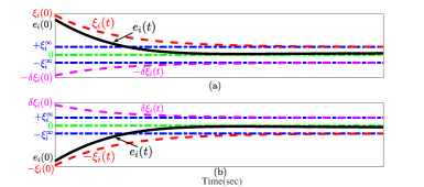
with δ[0,1]𝛿01\delta\in\left[0,1\right]. For clarity, define 𝒆i:=𝒆i(t)assignsubscript𝒆𝑖subscript𝒆𝑖𝑡\boldsymbol{e}_{i}:=\boldsymbol{e}_{i}\left(t\right) and ξi:=ξi(t)assignsubscript𝜉𝑖subscript𝜉𝑖𝑡\xi_{i}:=\xi_{i}\left(t\right). Also, let us define ξ=[ξ1,ξ2,ξ3,ξ4]𝜉superscriptsubscript𝜉1subscript𝜉2subscript𝜉3subscript𝜉4top\xi=[\xi_{1},\xi_{2},\xi_{3},\xi_{4}]^{\top}, =[1,2,3,4]superscriptsubscript1subscript2subscript3subscript4top\ell=[\ell_{1},\ell_{2},\ell_{3},\ell_{4}]^{\top}, ξ0=[ξ10,ξ20,ξ30,ξ40]superscript𝜉0superscriptsuperscriptsubscript𝜉10superscriptsubscript𝜉20superscriptsubscript𝜉30superscriptsubscript𝜉40top\xi^{0}=\left[\xi_{1}^{0},\xi_{2}^{0},\xi_{3}^{0},\xi_{4}^{0}\right]^{\top}, and ξ=[ξ1,ξ2,ξ3,ξ4]superscript𝜉superscriptsuperscriptsubscript𝜉1superscriptsubscript𝜉2superscriptsubscript𝜉3superscriptsubscript𝜉4top\xi^{\infty}=\left[\xi_{1}^{\infty},\xi_{2}^{\infty},\xi_{3}^{\infty},\xi_{4}^{\infty}\right]^{\top} for all ξ,,ξ0,ξ4𝜉superscript𝜉0superscript𝜉superscript4\xi,\ell,\xi^{0},\xi^{\infty}\in\mathbb{R}^{4}. The systematic convergence of the tracking error 𝒆isubscript𝒆𝑖\boldsymbol{e}_{i}, from a given large set to a given narrow set in accordance with (36) and (37) is depicted in Fig. 2.
Refer to caption
Figure 2: Graphical representation of the systematic convergence of tracking error 𝒆isubscript𝒆𝑖\boldsymbol{e}_{i} with PPF satisfying (a) Eq. (36); (b) Eq. (37).
Remark 1.

In accordance with the discussion in [25, 29], knowing the upper bound and the sign of 𝐞i(0)subscript𝐞𝑖0\boldsymbol{e}_{i}\left(0\right) is sufficient to force the error to satisfy the performance constraints and maintain the error regulation within predefined dynamically reducing boundaries for all t>0𝑡0t>0. If the condition in (36) or (37) is met, the maximum overshoot is sufficient to be bounded by ±δξiplus-or-minus𝛿subscript𝜉𝑖\pm\delta\xi_{i}, the steady-state error is bounded by ±ξiplus-or-minussuperscriptsubscript𝜉𝑖\pm\xi_{i}^{\infty}, and |𝐞i|subscript𝐞𝑖|\boldsymbol{e}_{i}| is trapped between ξisubscript𝜉𝑖\xi_{i} and δξi𝛿subscript𝜉𝑖\delta\xi_{i} as presented in Fig. 2.

Define the error 𝒆isubscript𝒆𝑖\boldsymbol{e}_{i} by

𝒆i=ξi𝒵(i)subscript𝒆𝑖subscript𝜉𝑖𝒵subscript𝑖\boldsymbol{e}_{i}=\xi_{i}\mathcal{Z}(\mathcal{E}_{i}) (38)

where ξisubscript𝜉𝑖\xi_{i}\in\mathbb{R} is defined in (35), isubscript𝑖\mathcal{E}_{i}\in\mathbb{R} is a relaxed form of the constrained error referred to as transformed error, and 𝒵(i)𝒵subscript𝑖\mathcal{Z}(\mathcal{E}_{i}) is a smooth function that behaves according to Assumption 2:

Assumption 2.

The smooth function 𝒵(i)𝒵subscript𝑖\mathcal{Z}(\mathcal{E}_{i}) has the following properties [25]:

  1. 1.

    𝒵(i)𝒵subscript𝑖\mathcal{Z}(\mathcal{E}_{i}) is smooth and strictly increasing.

  2. 2.

    𝒵(i)𝒵subscript𝑖\mathcal{Z}(\mathcal{E}_{i}) is constrained by the following two bounds
    δ¯i<𝒵(i)<δ¯i, if 𝒆i(0)0formulae-sequencesubscript¯𝛿𝑖𝒵subscript𝑖subscript¯𝛿𝑖 if subscript𝒆𝑖00-\underline{\delta}_{i}<\mathcal{Z}(\mathcal{E}_{i})<\bar{\delta}_{i},{\rm\text{ if }}\boldsymbol{e}_{i}\left(0\right)\geq 0
    δ¯i<𝒵(i)<δ¯i, if 𝒆i(0)<0formulae-sequencesubscript¯𝛿𝑖𝒵subscript𝑖subscript¯𝛿𝑖 if subscript𝒆𝑖00-\bar{\delta}_{i}<\mathcal{Z}(\mathcal{E}_{i})<\underline{\delta}_{i},{\rm\text{ if }}\boldsymbol{e}_{i}\left(0\right)<0
    with δ¯isubscript¯𝛿𝑖\bar{\delta}_{i} and δ¯isubscript¯𝛿𝑖\underline{\delta}_{i} being positive constants satisfy δ¯iδ¯isubscript¯𝛿𝑖subscript¯𝛿𝑖\underline{\delta}_{i}\leq\bar{\delta}_{i}.

  3. 3.
  4. limi𝒵(i)=δ¯ilimi+𝒵(i)=δ¯i} if 𝒆i0casessubscript𝑖𝒵subscript𝑖subscript¯𝛿𝑖subscript𝑖𝒵subscript𝑖subscript¯𝛿𝑖 if subscript𝒆𝑖0\left.\begin{array}[]{c}\underset{\mathcal{E}_{i}\rightarrow-\infty}{\lim}\mathcal{Z}(\mathcal{E}_{i})=-\underline{\delta}_{i}\\ \underset{\mathcal{E}_{i}\rightarrow+\infty}{\lim}\mathcal{Z}(\mathcal{E}_{i})=\bar{\delta}_{i}\end{array}\right\}{\rm\text{ if }}\boldsymbol{e}_{i}\geq 0
    limi𝒵(i)=δ¯ilimi+𝒵(i)=δ¯i} if 𝒆i<0casessubscript𝑖𝒵subscript𝑖subscript¯𝛿𝑖subscript𝑖𝒵subscript𝑖subscript¯𝛿𝑖 if subscript𝒆𝑖0\left.\begin{array}[]{c}\underset{\mathcal{E}_{i}\rightarrow-\infty}{\lim}\mathcal{Z}(\mathcal{E}_{i})=-\bar{\delta}_{i}\\ \underset{\mathcal{E}_{i}\rightarrow+\infty}{\lim}\mathcal{Z}(\mathcal{E}_{i})=\underline{\delta}_{i}\end{array}\right\}{\rm\text{ if }}\boldsymbol{e}_{i}<0
    such that

𝒵(i)={δ¯iexp(i)δ¯iexp(i)exp(i)+exp(i),δ¯iδ¯i if 𝒆i0δ¯iexp(i)δ¯iexp(i)exp(i)+exp(i),δ¯iδ¯i if 𝒆i<0𝒵subscript𝑖casessubscript¯𝛿𝑖subscript𝑖subscript¯𝛿𝑖subscript𝑖subscript𝑖subscript𝑖subscript¯𝛿𝑖subscript¯𝛿𝑖 if subscript𝒆𝑖0subscript¯𝛿𝑖subscript𝑖subscript¯𝛿𝑖subscript𝑖subscript𝑖subscript𝑖subscript¯𝛿𝑖subscript¯𝛿𝑖 if subscript𝒆𝑖0\mathcal{Z}\left(\mathcal{E}_{i}\right)=\begin{cases}\frac{\bar{\delta}_{i}\exp(\mathcal{E}_{i})-\underline{\delta}_{i}\exp(-\mathcal{E}_{i})}{\exp(\mathcal{E}_{i})+\exp(-\mathcal{E}_{i})},&\bar{\delta}_{i}\geq\underline{\delta}_{i}\text{ if }\boldsymbol{e}_{i}\geq 0\\ \frac{\bar{\delta}_{i}\exp(\mathcal{E}_{i})-\underline{\delta}_{i}\exp(-\mathcal{E}_{i})}{\exp(\mathcal{E}_{i})+\exp(-\mathcal{E}_{i})},&\underline{\delta}_{i}\geq\bar{\delta}_{i}\text{ if }\boldsymbol{e}_{i}<0\end{cases} (39)

The transformed error could be extracted through the inverse transformation of (39)

i(𝒆i,ξi)=𝒵1(𝒆i/ξi)subscript𝑖subscript𝒆𝑖subscript𝜉𝑖superscript𝒵1subscript𝒆𝑖subscript𝜉𝑖\mathcal{E}_{i}(\boldsymbol{e}_{i},\xi_{i})=\mathcal{Z}^{-1}(\boldsymbol{e}_{i}/\xi_{i}) (40)

with isubscript𝑖\mathcal{E}_{i}\in\mathbb{R}, 𝒵𝒵\mathcal{Z}\in\mathbb{R} and 𝒵1superscript𝒵1\mathcal{Z}^{-1}\in\mathbb{R} being smooth functions. For simplicity, let i:=i(,)assignsubscript𝑖subscript𝑖\mathcal{E}_{i}:=\mathcal{E}_{i}(\cdot,\cdot), δ¯=[δ¯1,δ¯2,δ¯3,δ¯4]¯𝛿superscriptsubscript¯𝛿1subscript¯𝛿2subscript¯𝛿3subscript¯𝛿4top\bar{\delta}=[\bar{\delta}_{1},\bar{\delta}_{2},\bar{\delta}_{3},\bar{\delta}_{4}]^{\top}, δ¯=[δ¯1,δ¯2,δ¯3,δ¯4]¯𝛿superscriptsubscript¯𝛿1subscript¯𝛿2subscript¯𝛿3subscript¯𝛿4top\underline{\delta}=[\underline{\delta}_{1},\underline{\delta}_{2},\underline{\delta}_{3},\underline{\delta}_{4}]^{\top}, =[R,P]superscriptsubscript𝑅superscriptsubscript𝑃toptop\mathcal{E}=\left[\mathcal{E}_{R},\mathcal{E}_{P}^{\top}\right]^{\top} for all δ¯,δ¯,4¯𝛿¯𝛿superscript4\bar{\delta},\underline{\delta},\mathcal{E}\in\mathbb{R}^{4} with R=1subscript𝑅subscript1\mathcal{E}_{R}=\mathcal{E}_{1}\in\mathbb{R} and P=[2,3,4]3subscript𝑃superscriptsubscript2subscript3subscript4topsuperscript3\mathcal{E}_{P}=[\mathcal{E}_{2},\mathcal{E}_{3},\mathcal{E}_{4}]^{\top}\in\mathbb{R}^{3}. In fact, the transformed error isubscript𝑖\mathcal{E}_{i} translates 𝒆isubscript𝒆𝑖\boldsymbol{e}_{i} from the given constrained form in (36) or (37) to its unconstrained form as in (40). From (39), the inverse transformation can be expressed as

i=subscript𝑖absent\displaystyle\mathcal{E}_{i}= 12{lnδ¯i+𝒆i/ξiδ¯i𝒆i/ξi,δ¯iδ¯i if 𝒆i0lnδ¯i+𝒆i/ξiδ¯i𝒆i/ξi,δ¯iδ¯i if 𝒆i<012caseslnsubscript¯𝛿𝑖subscript𝒆𝑖subscript𝜉𝑖subscript¯𝛿𝑖subscript𝒆𝑖subscript𝜉𝑖subscript¯𝛿𝑖subscript¯𝛿𝑖 if subscript𝒆𝑖0lnsubscript¯𝛿𝑖subscript𝒆𝑖subscript𝜉𝑖subscript¯𝛿𝑖subscript𝒆𝑖subscript𝜉𝑖subscript¯𝛿𝑖subscript¯𝛿𝑖 if subscript𝒆𝑖0\displaystyle\frac{1}{2}\begin{cases}\text{ln}\frac{\underline{\delta}_{i}+\boldsymbol{e}_{i}/\xi_{i}}{\bar{\delta}_{i}-\boldsymbol{e}_{i}/\xi_{i}},&\bar{\delta}_{i}\geq\underline{\delta}_{i}\text{ if }\boldsymbol{e}_{i}\geq 0\\ \text{ln}\frac{\underline{\delta}_{i}+\boldsymbol{e}_{i}/\xi_{i}}{\bar{\delta}_{i}-\boldsymbol{e}_{i}/\xi_{i}},&\underline{\delta}_{i}\geq\bar{\delta}_{i}\text{ if }\boldsymbol{e}_{i}<0\end{cases} (41)
Remark 2.

Consider the transformed error in (41). The transient and steady-state performance of the tracking error (𝐞isubscript𝐞𝑖\boldsymbol{e}_{i}) is bounded by the performance function ξisubscript𝜉𝑖\xi_{i}, and therefore, the prescribed performance is achieved if and only if isubscript𝑖\mathcal{E}_{i} is guaranteed to be bounded for all t0𝑡0t\geq 0.

Proposition 1.

Consider the error vector in (34) with the normalized Euclidean distance error R~Isubscriptnorm~𝑅𝐼||\tilde{R}||_{I} being given by (4). From (38), (39), and (40) let the transformed error be expressed as in (41) provided that δ¯=δ¯¯𝛿¯𝛿\underline{\delta}=\bar{\delta}. Then the following statements are true.

  1. (i)

    The only possible representation of 1subscript1\mathcal{E}_{1} is as follows:

    1=12lnδ¯1+𝒆1/ξ1δ¯1𝒆1/ξ1=12lnδ¯1+R~I/ξ1δ¯1R~I/ξ1subscript112lnsubscript¯𝛿1subscript𝒆1subscript𝜉1subscript¯𝛿1subscript𝒆1subscript𝜉112lnsubscript¯𝛿1subscriptnorm~𝑅𝐼subscript𝜉1subscript¯𝛿1subscriptnorm~𝑅𝐼subscript𝜉1\mathcal{E}_{1}=\frac{1}{2}\text{ln}\frac{\underline{\delta}_{1}+\boldsymbol{e}_{1}/\xi_{1}}{\bar{\delta}_{1}-\boldsymbol{e}_{1}/\xi_{1}}=\frac{1}{2}\text{ln}\frac{\underline{\delta}_{1}+||\tilde{R}||_{I}/\xi_{1}}{\bar{\delta}_{1}-||\tilde{R}||_{I}/\xi_{1}} (42)
  2. (ii)

    The transformed error 1>0R~I0subscript10for-allsubscriptnorm~𝑅𝐼0\mathcal{E}_{1}>0\forall||\tilde{R}||_{I}\neq 0.

  3. (iii)

    =𝟎¯4subscript¯04\mathcal{E}=\underline{\mathbf{0}}_{4} only at 𝒆=𝟎¯4𝒆subscript¯04\boldsymbol{e}=\underline{\mathbf{0}}_{4} and the critical point of \mathcal{E} satisfies 𝒆=𝟎¯4𝒆subscript¯04\boldsymbol{e}=\underline{\mathbf{0}}_{4}.

  4. (iv)

    The only critical point of \mathcal{E} is 𝑻~=𝐈4~𝑻subscript𝐈4\tilde{\boldsymbol{T}}=\mathbf{I}_{4}.

Proof. Given that 0R~(t)I1,t0formulae-sequence0subscriptnorm~𝑅𝑡𝐼1for-all𝑡00\leq||\tilde{R}\left(t\right)||_{I}\leq 1,\forall t\geq 0 as defined in (4), one can find that the upper part of (41) holds t0for-all𝑡0\forall t\geq 0 which proves (i). Since δ¯=δ¯¯𝛿¯𝛿\underline{\delta}=\bar{\delta} with the constraint R~Iξ1subscriptnorm~𝑅𝐼subscript𝜉1||\tilde{R}||_{I}\leq\xi_{1}, the expression in (42) is (δ¯1+R~I/ξ1)/(δ¯1R~I/ξ1)1R~I0subscript¯𝛿1subscriptnorm~𝑅𝐼subscript𝜉1subscript¯𝛿1subscriptnorm~𝑅𝐼subscript𝜉11for-allsubscriptnorm~𝑅𝐼0(\underline{\delta}_{1}+||\tilde{R}||_{I}/\xi_{1})/(\bar{\delta}_{1}-||\tilde{R}||_{I}/\xi_{1})\geq 1\forall||\tilde{R}||_{I}\neq 0. Thus, 1>0R~I0subscript10for-allsubscriptnorm~𝑅𝐼0\mathcal{E}_{1}>0\forall||\tilde{R}||_{I}\neq 0 which confirms (ii). Considering δ¯=δ¯¯𝛿¯𝛿\underline{\delta}=\bar{\delta} with the constraint 𝒆iξisubscript𝒆𝑖subscript𝜉𝑖\boldsymbol{e}_{i}\leq\xi_{i}, it is clear that (δ¯i+𝒆i/ξi)/(δ¯i𝒆i/ξi)=1subscript¯𝛿𝑖subscript𝒆𝑖subscript𝜉𝑖subscript¯𝛿𝑖subscript𝒆𝑖subscript𝜉𝑖1(\underline{\delta}_{i}+\boldsymbol{e}_{i}/\xi_{i})/(\bar{\delta}_{i}-\boldsymbol{e}_{i}/\xi_{i})=1 if and only if 𝒆i=0subscript𝒆𝑖0\boldsymbol{e}_{i}=0. Accordingly, i0𝒆i0subscript𝑖0for-allsubscript𝒆𝑖0\mathcal{E}_{i}\neq 0\forall\boldsymbol{e}_{i}\neq 0 and i=0subscript𝑖0\mathcal{E}_{i}=0 only at 𝒆i=0subscript𝒆𝑖0\boldsymbol{e}_{i}=0 which proves (iii). For (iv), from (4) and (31), R~I=0subscriptnorm~𝑅𝐼0||\tilde{R}||_{I}=0 and P~=0~𝑃0\tilde{P}=0 if and only if 𝑻~=𝐈4~𝑻subscript𝐈4\tilde{\boldsymbol{T}}=\mathbf{I}_{4}. Thus, the critical point of \mathcal{E} satisfies R~I=0subscriptnorm~𝑅𝐼0||\tilde{R}||_{I}=0 and P~=0~𝑃0\tilde{P}=0 which in turn satisfies 𝑻~=𝐈4~𝑻subscript𝐈4\tilde{\boldsymbol{T}}=\mathbf{I}_{4} and proves (iv). Define μi:=μi(𝒆i,ξi)assignsubscript𝜇𝑖subscript𝜇𝑖subscript𝒆𝑖subscript𝜉𝑖\mu_{i}:=\mu_{i}\left(\boldsymbol{e}_{i},\xi_{i}\right) such that

μi=12ξi𝒵1(𝒆i/ξi)(𝒆i/ξi)=12ξi(1δ¯i+𝒆i/ξi+1δ¯i𝒆i/ξi)subscript𝜇𝑖12subscript𝜉𝑖superscript𝒵1subscript𝒆𝑖subscript𝜉𝑖subscript𝒆𝑖subscript𝜉𝑖12subscript𝜉𝑖1subscript¯𝛿𝑖subscript𝒆𝑖subscript𝜉𝑖1subscript¯𝛿𝑖subscript𝒆𝑖subscript𝜉𝑖\begin{split}\mu_{i}&=\frac{1}{2\xi_{i}}\frac{\partial\mathcal{Z}^{-1}\left(\boldsymbol{e}_{i}/\xi_{i}\right)}{\partial\left(\boldsymbol{e}_{i}/\xi_{i}\right)}=\frac{1}{2\xi_{i}}\left(\frac{1}{\underline{\delta}_{i}+\boldsymbol{e}_{i}/\xi_{i}}+\frac{1}{\bar{\delta}_{i}-\boldsymbol{e}_{i}/\xi_{i}}\right)\end{split} (43)

Hence, one can find that the derivative of i˙˙subscript𝑖\dot{\mathcal{E}_{i}} is as follows:

i˙˙subscript𝑖\displaystyle\dot{\mathcal{E}_{i}} =μi(𝒆˙iξ˙iξi𝒆i)absentsubscript𝜇𝑖subscript˙𝒆𝑖subscript˙𝜉𝑖subscript𝜉𝑖subscript𝒆𝑖\displaystyle=\mu_{i}\left(\dot{\boldsymbol{e}}_{i}-\frac{\dot{\xi}_{i}}{\xi_{i}}\boldsymbol{e}_{i}\right) (44)

More simply, the expression in (44) is

˙=[𝚿R𝟎¯3𝟎¯3𝚿P](𝒆˙[𝚲R𝟎¯3𝟎¯3𝚲P]𝒆)˙delimited-[]subscript𝚿𝑅superscriptsubscript¯03topsubscript¯03subscript𝚿𝑃˙𝒆delimited-[]subscript𝚲𝑅superscriptsubscript¯03topsubscript¯03subscript𝚲𝑃𝒆\dot{\mathcal{E}}=\left[\begin{array}[]{cc}\boldsymbol{\Psi}_{R}&\underline{\mathbf{0}}_{3}^{\top}\\ \underline{\mathbf{0}}_{3}&\boldsymbol{\Psi}_{P}\end{array}\right]\left(\dot{\boldsymbol{e}}-\left[\begin{array}[]{cc}\boldsymbol{\Lambda}_{R}&\underline{\mathbf{0}}_{3}^{\top}\\ \underline{\mathbf{0}}_{3}&\boldsymbol{\Lambda}_{P}\end{array}\right]\boldsymbol{e}\right) (45)

with 𝚲R=ξ˙1ξ1subscript𝚲𝑅subscript˙𝜉1subscript𝜉1\boldsymbol{\Lambda}_{R}=\frac{\dot{\xi}_{1}}{\xi_{1}}, 𝚲P=diag(ξ˙2ξ2,ξ˙3ξ3,ξ˙4ξ4)subscript𝚲𝑃diagsubscript˙𝜉2subscript𝜉2subscript˙𝜉3subscript𝜉3subscript˙𝜉4subscript𝜉4\boldsymbol{\Lambda}_{P}={\rm diag}\left(\frac{\dot{\xi}_{2}}{\xi_{2}},\frac{\dot{\xi}_{3}}{\xi_{3}},\frac{\dot{\xi}_{4}}{\xi_{4}}\right), 𝚿R=μ1subscript𝚿𝑅subscript𝜇1\boldsymbol{\Psi}_{R}=\mu_{1}, and 𝚿P=diag(μ2,μ3,μ4)subscript𝚿𝑃diagsubscript𝜇2subscript𝜇3subscript𝜇4\boldsymbol{\Psi}_{P}={\rm diag}(\mu_{2},\mu_{3},\mu_{4}) for all 𝚲R,𝚿Rsubscript𝚲𝑅subscript𝚿𝑅\boldsymbol{\Lambda}_{R},\boldsymbol{\Psi}_{R}\in\mathbb{R} and 𝚲P,𝚿P3×3subscript𝚲𝑃subscript𝚿𝑃superscript33\boldsymbol{\Lambda}_{P},\boldsymbol{\Psi}_{P}\in\mathbb{R}^{3\times 3}. The following section introduces two nonlinear pose filters on 𝕊𝔼(3)𝕊𝔼3\mathbb{SE}\left(3\right) with prescribed performance characteristics which for 0|𝒆i(0)|<ξi(0)0subscript𝒆𝑖0subscript𝜉𝑖00\leq\left|\boldsymbol{e}_{i}\left(0\right)\right|<\xi_{i}\left(0\right) guarantee i,t0formulae-sequencesubscript𝑖subscriptfor-all𝑡0\mathcal{E}_{i}\in\mathcal{L}_{\infty},\forall t\geq 0 and, therefore, satisfy (36) or (37).

IV Nonlinear Complementary Pose Filters On 𝕊𝔼(3)𝕊𝔼3\mathbb{SE}\left(3\right) with Prescribed Performance

This section aims to provide a comprehensive description of the two nonlinear complementary pose filters evolved on 𝕊𝔼(3)𝕊𝔼3\mathbb{SE}\left(3\right) with the error vector, introduced in (34), behaving in accordance with the predefined transient as well as steady-state measures specified by the user. The first proposed filter is named a semi-direct pose filter with prescribed performance and the second one is termed a direct pose filter with prescribed performance. The difference between the two lies in the fact that while the semi-direct filter requires both attitude and position to be reconstructed through a set of vectorial measurements given in (15) and (17) combined with the measurement of the group velocity vector as described in (22) and (23), the direct filter only utilizes the above-mentioned measurements in the filter design. The structure of the proposed pose filters described in the two subsequent subsections is nonlinear on the Lie group of 𝕊𝔼(3)𝕊𝔼3\mathbb{SE}\left(3\right) and is given by

𝑻^˙=𝑻^[𝒴^]˙^𝑻^𝑻subscriptdelimited-[]^𝒴\dot{\hat{\boldsymbol{T}}}=\hat{\boldsymbol{T}}[\hat{\mathcal{Y}}]_{\wedge}

with 𝒴^=[Ω^,V^]6^𝒴superscript^Ωtopsuperscript^𝑉topsuperscript6\hat{\mathcal{Y}}=[\hat{\Omega}^{\top},\hat{V}^{\top}]\in\mathbb{R}^{6} such that R^˙=R^[Ω^]×˙^𝑅^𝑅subscriptdelimited-[]^Ω\dot{\hat{R}}=\hat{R}[\hat{\Omega}]_{\times} and P^˙=R^V^˙^𝑃^𝑅^𝑉\dot{\hat{P}}=\hat{R}\hat{V}.

IV-A Semi-direct Pose Filter with Prescribed Performance

Recall the error in (34) 𝒆=[R~I,P~]𝒆superscriptsubscriptnorm~𝑅𝐼superscript~𝑃toptop\boldsymbol{e}=\left[||\tilde{R}||_{I},\tilde{P}^{\top}\right]^{\top}. Define 𝑻y=[RyPy𝟎¯31]subscript𝑻𝑦delimited-[]subscript𝑅𝑦subscript𝑃𝑦superscriptsubscript¯03top1\boldsymbol{T}_{y}=\left[\begin{array}[]{cc}R_{y}&P_{y}\\ \underline{\mathbf{0}}_{3}^{\top}&1\end{array}\right] as a reconstructed homogeneous transformation matrix of the true 𝑻𝑻\boldsymbol{T}. Rysubscript𝑅𝑦R_{y} corrupted by uncertain measurements can be reconstructed as in [1, 2] or for simplicity visit the Appendix in [3, 14]. From (18) and (19) Pysubscript𝑃𝑦P_{y} is reconstructed in the following manner

Pysubscript𝑃𝑦\displaystyle P_{y} =1i=1NLkiLi=1NLkiL(vi(L)Ryvi(L))absent1superscriptsubscript𝑖1subscript𝑁Lsuperscriptsubscript𝑘𝑖Lsuperscriptsubscript𝑖1subscript𝑁Lsuperscriptsubscript𝑘𝑖Lsuperscriptsubscriptv𝑖Lsubscript𝑅𝑦superscriptsubscriptv𝑖L\displaystyle=\frac{1}{\sum_{i=1}^{N_{{\rm L}}}k_{i}^{{\rm L}}}\sum_{i=1}^{N_{{\rm L}}}k_{i}^{{\rm L}}\left({\rm v}_{i}^{\mathcal{I}\left({\rm L}\right)}-R_{y}{\rm v}_{i}^{\mathcal{B}\left({\rm L}\right)}\right)
=𝒢cRy𝒢cabsentsuperscriptsubscript𝒢𝑐subscript𝑅𝑦superscriptsubscript𝒢𝑐\displaystyle=\mathcal{G}_{c}^{\mathcal{I}}-R_{y}\mathcal{G}_{c}^{\mathcal{B}} (46)

Consider the following pose filter design

R^˙=˙^𝑅absent\displaystyle\dot{\hat{R}}= R^[Ωmb^ΩR^WΩ]×^𝑅subscriptdelimited-[]subscriptΩ𝑚subscript^𝑏Ωsuperscript^𝑅topsubscript𝑊Ω\displaystyle\hat{R}\left[\Omega_{m}-\hat{b}_{\Omega}-\hat{R}^{\top}W_{\Omega}\right]_{\times} (47)
P^˙=˙^𝑃absent\displaystyle\dot{\hat{P}}= R^(Vmb^VWV)^𝑅subscript𝑉𝑚subscript^𝑏𝑉subscript𝑊𝑉\displaystyle\hat{R}(V_{m}-\hat{b}_{V}-W_{V}) (48)
b^˙Ω=subscript˙^𝑏Ωabsent\displaystyle\dot{\hat{b}}_{\Omega}= γ2𝚿RRR^𝐯𝐞𝐱(𝓟a(R~))𝛾2subscript𝚿𝑅subscript𝑅superscript^𝑅top𝐯𝐞𝐱subscript𝓟𝑎~𝑅\displaystyle\frac{\gamma}{2}\boldsymbol{\Psi}_{R}\mathcal{E}_{R}\hat{R}^{\top}\mathbf{vex}(\boldsymbol{\mathcal{P}}_{a}(\tilde{R}))
+γR^[P~P^]×𝚿PP𝛾superscript^𝑅topsubscriptdelimited-[]~𝑃^𝑃subscript𝚿𝑃subscript𝑃\displaystyle+\gamma\hat{R}^{\top}\left[\tilde{P}-\hat{P}\right]_{\times}\boldsymbol{\Psi}_{P}\mathcal{E}_{P} (49)
b^˙V=subscript˙^𝑏𝑉absent\displaystyle\dot{\hat{b}}_{V}= γR^𝚿PP𝛾superscript^𝑅topsubscript𝚿𝑃subscript𝑃\displaystyle\gamma\hat{R}^{\top}\boldsymbol{\Psi}_{P}\mathcal{E}_{P} (50)
WΩ=subscript𝑊Ωabsent\displaystyle W_{\Omega}= 2kw𝚿RR𝚲R/41R~I𝐯𝐞𝐱(𝓟a(R~))2subscript𝑘𝑤subscript𝚿𝑅subscript𝑅subscript𝚲𝑅41subscriptnorm~𝑅𝐼𝐯𝐞𝐱subscript𝓟𝑎~𝑅\displaystyle 2\frac{k_{w}\boldsymbol{\Psi}_{R}\mathcal{E}_{R}-\boldsymbol{\Lambda}_{R}/4}{1-||\tilde{R}||_{I}}\mathbf{vex}(\boldsymbol{\mathcal{P}}_{a}(\tilde{R})) (51)
WV=subscript𝑊𝑉absent\displaystyle W_{V}= R^(kw𝚿PP+[P~P^]×WΩ𝚲PP~)superscript^𝑅topsubscript𝑘𝑤subscript𝚿𝑃subscript𝑃subscriptdelimited-[]~𝑃^𝑃subscript𝑊Ωsubscript𝚲𝑃~𝑃\displaystyle\hat{R}^{\top}\left(k_{w}\boldsymbol{\Psi}_{P}\mathcal{E}_{P}+\left[\tilde{P}-\hat{P}\right]_{\times}W_{\Omega}-\boldsymbol{\Lambda}_{P}\tilde{P}\right) (52)

with R~=R^Ry~𝑅^𝑅superscriptsubscript𝑅𝑦top\tilde{R}=\hat{R}R_{y}^{\top}, P~=P^R~Py~𝑃^𝑃~𝑅subscript𝑃𝑦\tilde{P}=\hat{P}-\tilde{R}P_{y}, Rsubscript𝑅\mathcal{E}_{R}, Psubscript𝑃\mathcal{E}_{P}, 𝚿Rsubscript𝚿𝑅\boldsymbol{\Psi}_{R} and 𝚿Psubscript𝚿𝑃\boldsymbol{\Psi}_{P} being defined in (43), and (44), respectively, kwsubscript𝑘𝑤k_{w} and γ𝛾\gamma being positive constants, and each of b^Ωsubscript^𝑏Ω\hat{b}_{\Omega} and b^Vsubscript^𝑏𝑉\hat{b}_{V} being the estimates of bΩsubscript𝑏Ωb_{\Omega} and bVsubscript𝑏𝑉b_{V}, respectively. The equivalent quaternion representation and complete implementation steps of the semi-direct filter are given in Appendix B.

Define the error between the true and the estimated bias by

b~Ωsubscript~𝑏Ω\displaystyle\tilde{b}_{\Omega} =bΩb^Ωabsentsubscript𝑏Ωsubscript^𝑏Ω\displaystyle=b_{\Omega}-\hat{b}_{\Omega} (53)
b~Vsubscript~𝑏𝑉\displaystyle\tilde{b}_{V} =bVb^Vabsentsubscript𝑏𝑉subscript^𝑏𝑉\displaystyle=b_{V}-\hat{b}_{V} (54)

where b~=[b~Ω,b~V]6~𝑏superscriptsuperscriptsubscript~𝑏Ωtopsuperscriptsubscript~𝑏𝑉toptopsuperscript6\tilde{b}=\left[\tilde{b}_{\Omega}^{\top},\tilde{b}_{V}^{\top}\right]^{\top}\in\mathbb{R}^{6} is the group error bias vector.

Theorem 1.

Consider the pose dynamics in (21), the group of noise-free velocity measurements in (22) and (23) such that Ωm=Ω+bΩsubscriptΩ𝑚Ωsubscript𝑏Ω\Omega_{m}=\Omega+b_{\Omega} and Vm=V+bVsubscript𝑉𝑚𝑉subscript𝑏𝑉V_{m}=V+b_{V}, in addition to other vector measurements given in (15) and (17) coupled with the filter kinematics in (47), (48), (49), (50), (51), and (52). Let Assumption 1 hold. Define 𝒰𝕊𝔼(3)×6𝒰𝕊𝔼3superscript6\mathcal{U}\subseteq\mathbb{SE}\left(3\right)\times\mathbb{R}^{6} by 𝒰:={(𝐓~(0),b~(0))|Tr{R~(0)}=1,P~(0)=𝟎¯3,b~(0)=𝟎¯6}assign𝒰conditional-set~𝐓0~𝑏0formulae-sequenceTr~𝑅01formulae-sequence~𝑃0subscript¯03~𝑏0subscript¯06\mathcal{U}:=\left\{\left.(\tilde{\boldsymbol{T}}\left(0\right),\tilde{b}\left(0\right))\right|{\rm Tr}\{\tilde{R}\left(0\right)\}=-1,\tilde{P}\left(0\right)=\underline{\mathbf{0}}_{3},\tilde{b}\left(0\right)=\underline{\mathbf{0}}_{6}\right\}. From almost any initial condition such that Tr{R~(0)}𝒰Tr~𝑅0𝒰{\rm Tr}\{\tilde{R}\left(0\right)\}\notin\mathcal{U} and (0)0subscript\mathcal{E}\left(0\right)\in\mathcal{L}_{\infty}, all signals in the closed loop are bounded, limt(t)=0subscript𝑡𝑡0\lim_{t\rightarrow\infty}\mathcal{E}\left(t\right)=0, and 𝐓~~𝐓\tilde{\boldsymbol{T}} asymptotically approaches 𝐈4subscript𝐈4\mathbf{I}_{4}.

Theorem 1 guarantees that the observer pose dynamics in (47), (48), (49), (50), (51), and (52) are stable with (t)𝑡\mathcal{E}\left(t\right) asymptotically approaching the origin. Since (t)𝑡\mathcal{E}\left(t\right) is bounded, the error vector 𝒆𝒆\boldsymbol{e} in (34) is constrained by the transient and steady-state boundaries introduced in (35).

Proof. Consider the error in the homogeneous transformation matrix from body-frame to estimator-frame defined as (31). From (20) and (47) the error dynamics are

R~˙˙~𝑅\displaystyle\dot{\tilde{R}} =R^[b~ΩR^WΩ]×R=[R^b~ΩWΩ]×R~absent^𝑅subscriptdelimited-[]subscript~𝑏Ωsuperscript^𝑅topsubscript𝑊Ωsuperscript𝑅topsubscriptdelimited-[]^𝑅subscript~𝑏Ωsubscript𝑊Ω~𝑅\displaystyle=\hat{R}\left[\tilde{b}_{\Omega}-\hat{R}^{\top}W_{\Omega}\right]_{\times}R^{\top}=\left[\hat{R}\tilde{b}_{\Omega}-W_{\Omega}\right]_{\times}\tilde{R} (55)

where [R^b~Ω]×=R^[b~Ω]×R^subscriptdelimited-[]^𝑅subscript~𝑏Ω^𝑅subscriptdelimited-[]subscript~𝑏Ωsuperscript^𝑅top\left[\hat{R}\tilde{b}_{\Omega}\right]_{\times}=\hat{R}\left[\tilde{b}_{\Omega}\right]_{\times}\hat{R}^{\top} as given in identity (7). In view of (20) and (24), one can express the error dynamics in (55) in terms of normalized Euclidean distance as

ddtR~I𝑑𝑑𝑡subscriptnorm~𝑅𝐼\displaystyle\frac{d}{dt}||\tilde{R}||_{I} =ddt14Tr{𝐈3R~}absent𝑑𝑑𝑡14Trsubscript𝐈3~𝑅\displaystyle=\frac{d}{dt}\frac{1}{4}{\rm Tr}\{\mathbf{I}_{3}-\tilde{R}\}
=14Tr{[R^b~ΩWΩ]×𝓟a(R~)}absent14Trsubscriptdelimited-[]^𝑅subscript~𝑏Ωsubscript𝑊Ωsubscript𝓟𝑎~𝑅\displaystyle=-\frac{1}{4}{\rm Tr}\left\{\left[\hat{R}\tilde{b}_{\Omega}-W_{\Omega}\right]_{\times}\boldsymbol{\mathcal{P}}_{a}(\tilde{R})\right\}
=12𝐯𝐞𝐱(𝓟a(R~))(R^b~ΩWΩ)absent12𝐯𝐞𝐱superscriptsubscript𝓟𝑎~𝑅top^𝑅subscript~𝑏Ωsubscript𝑊Ω\displaystyle=\frac{1}{2}\mathbf{vex}(\boldsymbol{\mathcal{P}}_{a}(\tilde{R}))^{\top}(\hat{R}\tilde{b}_{\Omega}-W_{\Omega}) (56)

with Tr{R~[b~W]×}=2𝐯𝐞𝐱(𝓟a(R~))(b~W)Tr~𝑅subscriptdelimited-[]~𝑏𝑊2𝐯𝐞𝐱superscriptsubscript𝓟𝑎~𝑅top~𝑏𝑊{\rm Tr}\left\{\tilde{R}\left[\tilde{b}-W\right]_{\times}\right\}=-2\mathbf{vex}(\boldsymbol{\mathcal{P}}_{a}(\tilde{R}))^{\top}(\tilde{b}-W) being defined in (11). Since the position error is given by P~=P^R~P~𝑃^𝑃~𝑅𝑃\tilde{P}=\hat{P}-\tilde{R}P in (31), one can find the derivative of P~~𝑃\tilde{P} to be

P~˙˙~𝑃\displaystyle\dot{\tilde{P}} =P^˙R~˙PR~P˙absent˙^𝑃˙~𝑅𝑃~𝑅˙𝑃\displaystyle=\dot{\hat{P}}-\dot{\tilde{R}}P-\tilde{R}\dot{P}
=P^˙[R^b~ΩWΩ]×R~PR~R(VmbV)absent˙^𝑃subscriptdelimited-[]^𝑅subscript~𝑏Ωsubscript𝑊Ω~𝑅𝑃~𝑅𝑅subscript𝑉𝑚subscript𝑏𝑉\displaystyle=\dot{\hat{P}}-\left[\hat{R}\tilde{b}_{\Omega}-W_{\Omega}\right]_{\times}\tilde{R}P-\tilde{R}R(V_{m}-b_{V})
=R^(b~VWV)+[P^P~]×(R^b~ΩWΩ)absent^𝑅subscript~𝑏𝑉subscript𝑊𝑉subscriptdelimited-[]^𝑃~𝑃^𝑅subscript~𝑏Ωsubscript𝑊Ω\displaystyle=\hat{R}(\tilde{b}_{V}-W_{V})+\left[\hat{P}-\tilde{P}\right]_{\times}(\hat{R}\tilde{b}_{\Omega}-W_{\Omega}) (57)

with [R^b~Ω]×P^=[P^]×R^b~Ωsubscriptdelimited-[]^𝑅subscript~𝑏Ω^𝑃subscriptdelimited-[]^𝑃^𝑅subscript~𝑏Ω\left[\hat{R}\tilde{b}_{\Omega}\right]_{\times}\hat{P}=-\left[\hat{P}\right]_{\times}\hat{R}\tilde{b}_{\Omega}. From (56) and (57), and in view of (25), the dynamics of the error vector in (34) become

[R~˙IP~˙]delimited-[]subscriptnorm˙~𝑅𝐼˙~𝑃\displaystyle\left[\begin{array}[]{c}||\dot{\tilde{R}}||_{I}\\ \dot{\tilde{P}}\end{array}\right] =[12𝐯𝐞𝐱(𝓟a(R~))𝟎¯3[P^P~]×R^][R^b~ΩWΩb~VWV]absentdelimited-[]12𝐯𝐞𝐱superscriptsubscript𝓟𝑎~𝑅topsuperscriptsubscript¯03topsubscriptdelimited-[]^𝑃~𝑃^𝑅delimited-[]^𝑅subscript~𝑏Ωsubscript𝑊Ωsubscript~𝑏𝑉subscript𝑊𝑉\displaystyle=\left[\begin{array}[]{cc}\frac{1}{2}\mathbf{vex}(\boldsymbol{\mathcal{P}}_{a}(\tilde{R}))^{\top}&\underline{\mathbf{0}}_{3}^{\top}\\ \left[\hat{P}-\tilde{P}\right]_{\times}&\hat{R}\end{array}\right]\left[\begin{array}[]{c}\hat{R}\tilde{b}_{\Omega}-W_{\Omega}\\ \tilde{b}_{V}-W_{V}\end{array}\right] (64)

Accordingly, the derivative of the transformed error in (45) can be represented with direct substitution of 𝒆=[R~I,P~]𝒆superscriptsubscriptnorm~𝑅𝐼superscript~𝑃toptop\boldsymbol{e}=\left[||\tilde{R}||_{I},\tilde{P}^{\top}\right]^{\top} in addition to the result in (64). Now, consider the following candidate Lyapunov function

V(,b~Ω,b~V)𝑉subscript~𝑏Ωsubscript~𝑏𝑉\displaystyle V(\mathcal{E},\tilde{b}_{\Omega},\tilde{b}_{V}) =122+12γb~Ω2+12γb~V2absent12superscriptnorm212𝛾superscriptnormsubscript~𝑏Ω212𝛾superscriptnormsubscript~𝑏𝑉2\displaystyle=\frac{1}{2}||\mathcal{E}||^{2}+\frac{1}{2\gamma}||\tilde{b}_{\Omega}||^{2}+\frac{1}{2\gamma}||\tilde{b}_{V}||^{2} (65)

Differentiating V:=V(,b~Ω,b~V)assign𝑉𝑉subscript~𝑏Ωsubscript~𝑏𝑉V:=V(\mathcal{E},\tilde{b}_{\Omega},\tilde{b}_{V}) in (65) results in

V˙=˙𝑉absent\displaystyle\dot{V}= ˙1γb~Ωb^˙Ω1γb~Vb^˙Vsuperscripttop˙1𝛾superscriptsubscript~𝑏Ωtopsubscript˙^𝑏Ω1𝛾superscriptsubscript~𝑏𝑉topsubscript˙^𝑏𝑉\displaystyle\mathcal{E}^{\top}\dot{\mathcal{E}}-\frac{1}{\gamma}\tilde{b}_{\Omega}^{\top}\dot{\hat{b}}_{\Omega}-\frac{1}{\gamma}\tilde{b}_{V}^{\top}\dot{\hat{b}}_{V}
=\displaystyle= R𝚿R(12𝐯𝐞𝐱(𝓟a(R~))(R^b~ΩWΩ)𝚲RR~I)subscript𝑅subscript𝚿𝑅12𝐯𝐞𝐱superscriptsubscript𝓟𝑎~𝑅top^𝑅subscript~𝑏Ωsubscript𝑊Ωsubscript𝚲𝑅subscriptnorm~𝑅𝐼\displaystyle\mathcal{E}_{R}\boldsymbol{\Psi}_{R}\left(\frac{1}{2}\mathbf{vex}(\boldsymbol{\mathcal{P}}_{a}(\tilde{R}))^{\top}(\hat{R}\tilde{b}_{\Omega}-W_{\Omega})-\boldsymbol{\Lambda}_{R}||\tilde{R}||_{I}\right)
+P𝚿P(R^(b~VWV)+[P^P~]×(R^b~ΩWΩ))superscriptsubscript𝑃topsubscript𝚿𝑃^𝑅subscript~𝑏𝑉subscript𝑊𝑉subscriptdelimited-[]^𝑃~𝑃^𝑅subscript~𝑏Ωsubscript𝑊Ω\displaystyle+\mathcal{E}_{P}^{\top}\boldsymbol{\Psi}_{P}\left(\hat{R}(\tilde{b}_{V}-W_{V})+\left[\hat{P}-\tilde{P}\right]_{\times}(\hat{R}\tilde{b}_{\Omega}-W_{\Omega})\right)
P𝚿P𝚲PP~1γb~Ωb^˙Ω1γb~Vb^˙Vsuperscriptsubscript𝑃topsubscript𝚿𝑃subscript𝚲𝑃~𝑃1𝛾superscriptsubscript~𝑏Ωtopsubscript˙^𝑏Ω1𝛾superscriptsubscript~𝑏𝑉topsubscript˙^𝑏𝑉\displaystyle-\mathcal{E}_{P}^{\top}\boldsymbol{\Psi}_{P}\boldsymbol{\Lambda}_{P}\tilde{P}-\frac{1}{\gamma}\tilde{b}_{\Omega}^{\top}\dot{\hat{b}}_{\Omega}-\frac{1}{\gamma}\tilde{b}_{V}^{\top}\dot{\hat{b}}_{V} (66)

Consider R~I=14𝐯𝐞𝐱(𝓟a(R~))21R~Isubscriptnorm~𝑅𝐼14superscriptnorm𝐯𝐞𝐱subscript𝓟𝑎~𝑅21subscriptnorm~𝑅𝐼||\tilde{R}||_{I}=\frac{1}{4}\frac{||\mathbf{vex}(\boldsymbol{\mathcal{P}}_{a}(\tilde{R}))||^{2}}{1-||\tilde{R}||_{I}} as defined in (32). Using the result in (66) and directly substituting b^˙Ωsubscript˙^𝑏Ω\dot{\hat{b}}_{\Omega}, b^˙Vsubscript˙^𝑏𝑉\dot{\hat{b}}_{V}, WΩsubscript𝑊ΩW_{\Omega} and WVsubscript𝑊𝑉W_{V} with their definitions in (49), (50), (51), and (52), respectively, one obtains

V˙˙𝑉\displaystyle\dot{V} =14kwR2𝚿R2𝐯𝐞𝐱(𝓟a(R~))21R~IkwP𝚿P2Pabsent14subscript𝑘𝑤superscriptsubscript𝑅2superscriptsubscript𝚿𝑅2superscriptnorm𝐯𝐞𝐱subscript𝓟𝑎~𝑅21subscriptnorm~𝑅𝐼subscript𝑘𝑤superscriptsubscript𝑃topsuperscriptsubscript𝚿𝑃2subscript𝑃\displaystyle=-\frac{1}{4}k_{w}\mathcal{E}_{R}^{2}\boldsymbol{\Psi}_{R}^{2}\frac{||\mathbf{vex}(\boldsymbol{\mathcal{P}}_{a}(\tilde{R}))||^{2}}{1-||\tilde{R}||_{I}}-k_{w}\mathcal{E}_{P}^{\top}\boldsymbol{\Psi}_{P}^{2}\mathcal{E}_{P}
=kwR2𝚿R2R~IkwP𝚿P2Pabsentsubscript𝑘𝑤superscriptsubscript𝑅2superscriptsubscript𝚿𝑅2subscriptnorm~𝑅𝐼subscript𝑘𝑤superscriptsubscript𝑃topsuperscriptsubscript𝚿𝑃2subscript𝑃\displaystyle=-k_{w}\mathcal{E}_{R}^{2}\boldsymbol{\Psi}_{R}^{2}||\tilde{R}||_{I}-k_{w}\mathcal{E}_{P}^{\top}\boldsymbol{\Psi}_{P}^{2}\mathcal{E}_{P} (67)

The result obtained in (67) indicates that V(t)V(0),t0formulae-sequence𝑉𝑡𝑉0for-all𝑡0V\left(t\right)\leq V\left(0\right),\forall t\geq 0. Given that V(t)V(0),t0formulae-sequence𝑉𝑡𝑉0for-all𝑡0V\left(t\right)\leq V\left(0\right),\forall t\geq 0, R~(0)𝒰~𝑅0𝒰\tilde{R}\left(0\right)\notin\mathcal{U} and (0)40superscript4\mathcal{E}\left(0\right)\in\mathbb{R}^{4}, b~~𝑏\tilde{b} remains bounded, and \mathcal{E} is bounded and well defined for all t0𝑡0t\geq 0. Consequently, P~~𝑃\tilde{P}, R~Isubscriptnorm~𝑅𝐼||\tilde{R}||_{I} and 𝐯𝐞𝐱(𝓟a(R~))𝐯𝐞𝐱subscript𝓟𝑎~𝑅\mathbf{vex}(\boldsymbol{\mathcal{P}}_{a}(\tilde{R})) are bounded, which in turn signifies that P~˙˙~𝑃\dot{\tilde{P}}, R~˙Isubscriptnorm˙~𝑅𝐼||\dot{\tilde{R}}||_{I}, ˙Rsubscript˙𝑅\dot{\mathcal{E}}_{R} and ˙Psubscript˙𝑃\dot{\mathcal{E}}_{P} are bounded as well. From the result in (67) it follows that

V¨=¨𝑉absent\displaystyle\ddot{V}= kw(2R𝚿R(˙R𝚿R+R𝚿˙R)R~I+R2𝚿R2R~˙I)subscript𝑘𝑤2subscript𝑅subscript𝚿𝑅subscript˙𝑅subscript𝚿𝑅subscript𝑅subscript˙𝚿𝑅subscriptnorm~𝑅𝐼superscriptsubscript𝑅2superscriptsubscript𝚿𝑅2subscriptnorm˙~𝑅𝐼\displaystyle-k_{w}\left(2\mathcal{E}_{R}\boldsymbol{\Psi}_{R}(\dot{\mathcal{E}}_{R}\boldsymbol{\Psi}_{R}+\mathcal{E}_{R}\dot{\boldsymbol{\Psi}}_{R})||\tilde{R}||_{I}+\mathcal{E}_{R}^{2}\boldsymbol{\Psi}_{R}^{2}||\dot{\tilde{R}}||_{I}\right)
2kwP𝚿P2˙P2kwP𝚿P𝚿˙PP2subscript𝑘𝑤superscriptsubscript𝑃topsuperscriptsubscript𝚿𝑃2subscript˙𝑃2subscript𝑘𝑤superscriptsubscript𝑃topsubscript𝚿𝑃subscript˙𝚿𝑃subscript𝑃\displaystyle-2k_{w}\mathcal{E}_{P}^{\top}\boldsymbol{\Psi}_{P}^{2}\dot{\mathcal{E}}_{P}-2k_{w}\mathcal{E}_{P}^{\top}\boldsymbol{\Psi}_{P}\dot{\boldsymbol{\Psi}}_{P}\mathcal{E}_{P} (68)

Since 𝚿R=μ1subscript𝚿𝑅subscript𝜇1\boldsymbol{\Psi}_{R}=\mu_{1} and 𝚿P=diag(μ2,μ3,μ4)subscript𝚿𝑃diagsubscript𝜇2subscript𝜇3subscript𝜇4\boldsymbol{\Psi}_{P}={\rm diag}(\mu_{2},\mu_{3},\mu_{4}) defined in (43), μ˙isubscript˙𝜇𝑖\dot{\mu}_{i} can be expressed as follows for all i=1,2,,4𝑖124i=1,2,\ldots,4

μ˙i=subscript˙𝜇𝑖absent\displaystyle\dot{\mu}_{i}= 12δ¯iξ˙i+𝒆˙i(δ¯iξi+𝒆i)212δ¯iξ˙i𝒆˙i(δ¯iξi𝒆i)212subscript¯𝛿𝑖subscript˙𝜉𝑖subscript˙𝒆𝑖superscriptsubscript¯𝛿𝑖subscript𝜉𝑖subscript𝒆𝑖212subscript¯𝛿𝑖subscript˙𝜉𝑖subscript˙𝒆𝑖superscriptsubscript¯𝛿𝑖subscript𝜉𝑖subscript𝒆𝑖2\displaystyle-\frac{1}{2}\frac{\underline{\delta}_{i}\dot{\xi}_{i}+\dot{\boldsymbol{e}}_{i}}{(\underline{\delta}_{i}\xi_{i}+\boldsymbol{e}_{i})^{2}}-\frac{1}{2}\frac{\bar{\delta}_{i}\dot{\xi}_{i}-\dot{\boldsymbol{e}}_{i}}{(\bar{\delta}_{i}\xi_{i}-\boldsymbol{e}_{i})^{2}} (69)

with ξ˙i=i(ξi0ξi)exp(it)subscript˙𝜉𝑖subscript𝑖superscriptsubscript𝜉𝑖0superscriptsubscript𝜉𝑖subscript𝑖𝑡\dot{\xi}_{i}=-\ell_{i}(\xi_{i}^{0}-\xi_{i}^{\infty})\exp(-\ell_{i}t). Due to the fact that 𝒆˙isubscript˙𝒆𝑖\dot{\boldsymbol{e}}_{i} is bounded for all i=1,2,,4𝑖124i=1,2,\ldots,4, μ˙isubscript˙𝜇𝑖\dot{\mu}_{i} is bounded and V¨¨𝑉\ddot{V} in (68) is uniformly bounded for all t0𝑡0t\geq 0. It should be remarked that 1>0subscript10\mathcal{E}_{1}>0 for all R~I>0subscriptnorm~𝑅𝐼0||\tilde{R}||_{I}>0, and 10subscript10\mathcal{E}_{1}\rightarrow 0 as R~I0subscriptnorm~𝑅𝐼0||\tilde{R}||_{I}\rightarrow 0 and vice versa as stated in property (ii) of Proposition 1. In addition, i0𝒆i0subscript𝑖0for-allsubscript𝒆𝑖0\mathcal{E}_{i}\neq 0\forall\boldsymbol{e}_{i}\neq 0 and i=0subscript𝑖0\mathcal{E}_{i}=0 if and only if 𝒆i=0subscript𝒆𝑖0\boldsymbol{e}_{i}=0 as indicated in property (iii) of Proposition 1. Therefore, V˙˙𝑉\dot{V} is uniformly continuous, and in consistence with Barbalat Lemma, V˙0˙𝑉0\dot{V}\rightarrow 0 as t𝑡t\rightarrow\infty signifies that i0subscript𝑖0\mathcal{E}_{i}\rightarrow 0 and 𝒆i0subscript𝒆𝑖0\boldsymbol{e}_{i}\rightarrow 0. As mentioned by property (iv) of Proposition 1, 00\mathcal{E}\rightarrow 0 implies that 𝑻~~𝑻\tilde{\boldsymbol{T}} asymptotically approaches 𝐈4subscript𝐈4\mathbf{I}_{4} which completes the proof.

IV-B Direct Pose Filter with Prescribed Performance

The reconstructed homogeneous transformation matrix 𝑻ysubscript𝑻𝑦\boldsymbol{T}_{y} defined in Subsection IV-A consists of two elements: Rysubscript𝑅𝑦R_{y} and Pysubscript𝑃𝑦P_{y}. Although, Rysubscript𝑅𝑦R_{y} can be statically reconstructed applying, for example, QUEST [1], or SVD [2], the aforementioned methods of static reconstruction could significantly increase processing cost [9, 31]. Thus, the pose filter proposed in this Subsection avoids the necessity of attitude reconstruction and instead uses measurements from the inertial and body-frame units directly. Let us define

𝓜T=[𝐌T𝐦v𝐦v𝐦c]=subscript𝓜Tdelimited-[]subscript𝐌Tsubscript𝐦vsuperscriptsubscript𝐦vtopsubscript𝐦cabsent\displaystyle\boldsymbol{\mathcal{M}}_{{\rm T}}=\left[\begin{array}[]{cc}\mathbf{M}_{{\rm T}}&\mathbf{m}_{{\rm v}}\\ \mathbf{m}_{{\rm v}}^{\top}&\mathbf{m}_{{\rm c}}\end{array}\right]= i=1NRkiR[υi(R)0][υi(R)0]superscriptsubscript𝑖1subscript𝑁Rsuperscriptsubscript𝑘𝑖Rdelimited-[]superscriptsubscript𝜐𝑖R0superscriptdelimited-[]superscriptsubscript𝜐𝑖R0top\displaystyle\sum_{i=1}^{N_{{\rm R}}}k_{i}^{{\rm R}}\left[\begin{array}[]{c}\upsilon_{i}^{\mathcal{I}\left({\rm R}\right)}\\ 0\end{array}\right]\left[\begin{array}[]{c}\upsilon_{i}^{\mathcal{I}\left({\rm R}\right)}\\ 0\end{array}\right]^{\top} (76)
+j=1NLkjL[vj(L)1][vj(L)1]superscriptsubscript𝑗1subscript𝑁Lsuperscriptsubscript𝑘𝑗Ldelimited-[]superscriptsubscriptv𝑗L1superscriptdelimited-[]superscriptsubscriptv𝑗L1top\displaystyle+\sum_{j=1}^{N_{{\rm L}}}k_{j}^{{\rm L}}\left[\begin{array}[]{c}{\rm v}_{j}^{\mathcal{I}\left({\rm L}\right)}\\ 1\end{array}\right]\left[\begin{array}[]{c}{\rm v}_{j}^{\mathcal{I}\left({\rm L}\right)}\\ 1\end{array}\right]^{\top} (81)

such that 𝐌T=𝐌R+𝐌Lsubscript𝐌Tsubscript𝐌Rsubscript𝐌L\mathbf{M}_{{\rm T}}=\mathbf{M}_{{\rm R}}+\mathbf{M}_{{\rm L}} with

𝐌R=subscript𝐌Rabsent\displaystyle\mathbf{M}_{{\rm R}}= i=1NRkiRυi(R)(υi(R))superscriptsubscript𝑖1subscript𝑁Rsuperscriptsubscript𝑘𝑖Rsuperscriptsubscript𝜐𝑖Rsuperscriptsuperscriptsubscript𝜐𝑖Rtop\displaystyle\sum_{i=1}^{N_{{\rm R}}}k_{i}^{{\rm R}}\upsilon_{i}^{\mathcal{I}\left({\rm R}\right)}\left(\upsilon_{i}^{\mathcal{I}\left({\rm R}\right)}\right)^{\top}
𝐌L=subscript𝐌Labsent\displaystyle\mathbf{M}_{{\rm L}}= j=1NLkjLvj(L)(vj(L))superscriptsubscript𝑗1subscript𝑁Lsuperscriptsubscript𝑘𝑗Lsuperscriptsubscriptv𝑗Lsuperscriptsuperscriptsubscriptv𝑗Ltop\displaystyle\sum_{j=1}^{N_{{\rm L}}}k_{j}^{{\rm L}}{\rm v}_{j}^{\mathcal{I}\left({\rm L}\right)}\left({\rm v}_{j}^{\mathcal{I}\left({\rm L}\right)}\right)^{\top}
𝐦v=subscript𝐦vabsent\displaystyle\mathbf{m}_{{\rm v}}= j=1NLkjLvj(L)superscriptsubscript𝑗1subscript𝑁Lsuperscriptsubscript𝑘𝑗Lsuperscriptsubscriptv𝑗L\displaystyle\sum_{j=1}^{N_{{\rm L}}}k_{j}^{{\rm L}}{\rm v}_{j}^{\mathcal{I}\left({\rm L}\right)}
𝐦c=subscript𝐦cabsent\displaystyle\mathbf{m}_{{\rm c}}= j=1NLkjLsuperscriptsubscript𝑗1subscript𝑁Lsuperscriptsubscript𝑘𝑗L\displaystyle\sum_{j=1}^{N_{{\rm L}}}k_{j}^{{\rm L}} (82)

where kiRsuperscriptsubscript𝑘𝑖Rk_{i}^{{\rm R}} and kjLsuperscriptsubscript𝑘𝑗Lk_{j}^{{\rm L}} are constant gains of the confidence level of i𝑖ith and j𝑗jth sensor measurements, respectively. Define

𝓚T=[𝐊T𝐤v𝐦v𝐦c]=subscript𝓚Tdelimited-[]subscript𝐊Tsubscript𝐤vsuperscriptsubscript𝐦vtopsubscript𝐦cabsent\displaystyle\boldsymbol{\mathcal{K}}_{{\rm T}}=\left[\begin{array}[]{cc}\mathbf{K}_{{\rm T}}&\mathbf{k}_{{\rm v}}\\ \mathbf{m}_{{\rm v}}^{\top}&\mathbf{m}_{{\rm c}}\end{array}\right]= i=1NRkiR[υi(R)0][υi(R)0]superscriptsubscript𝑖1subscript𝑁Rsuperscriptsubscript𝑘𝑖Rdelimited-[]superscriptsubscript𝜐𝑖R0superscriptdelimited-[]superscriptsubscript𝜐𝑖R0top\displaystyle\sum_{i=1}^{N_{{\rm R}}}k_{i}^{{\rm R}}\left[\begin{array}[]{c}\upsilon_{i}^{\mathcal{B}\left({\rm R}\right)}\\ 0\end{array}\right]\left[\begin{array}[]{c}\upsilon_{i}^{\mathcal{I}\left({\rm R}\right)}\\ 0\end{array}\right]^{\top} (89)
+j=1NLkjL[vj(L)1][vj(L)1]superscriptsubscript𝑗1subscript𝑁Lsuperscriptsubscript𝑘𝑗Ldelimited-[]superscriptsubscriptv𝑗L1superscriptdelimited-[]superscriptsubscriptv𝑗L1top\displaystyle+\sum_{j=1}^{N_{{\rm L}}}k_{j}^{{\rm L}}\left[\begin{array}[]{c}{\rm v}_{j}^{\mathcal{B}\left({\rm L}\right)}\\ 1\end{array}\right]\left[\begin{array}[]{c}{\rm v}_{j}^{\mathcal{I}\left({\rm L}\right)}\\ 1\end{array}\right]^{\top} (94)

such that 𝐦v=j=1NLkjLvj(L)subscript𝐦vsuperscriptsubscript𝑗1subscript𝑁Lsuperscriptsubscript𝑘𝑗Lsuperscriptsubscriptv𝑗L\mathbf{m}_{{\rm v}}=\sum_{j=1}^{N_{{\rm L}}}k_{j}^{{\rm L}}{\rm v}_{j}^{\mathcal{I}\left({\rm L}\right)} and 𝐦c=j=1NLkjLsubscript𝐦csuperscriptsubscript𝑗1subscript𝑁Lsuperscriptsubscript𝑘𝑗L\mathbf{m}_{{\rm c}}=\sum_{j=1}^{N_{{\rm L}}}k_{j}^{{\rm L}} as defined in (82), and

𝐊Tsubscript𝐊T\displaystyle\mathbf{K}_{{\rm T}} =i=1NRkiRυi(R)(υi(R))+j=1NLkiLvj(L)(vj(L))absentsuperscriptsubscript𝑖1subscript𝑁Rsuperscriptsubscript𝑘𝑖Rsuperscriptsubscript𝜐𝑖Rsuperscriptsuperscriptsubscript𝜐𝑖Rtopsuperscriptsubscript𝑗1subscript𝑁Lsuperscriptsubscript𝑘𝑖Lsuperscriptsubscriptv𝑗Lsuperscriptsuperscriptsubscriptv𝑗Ltop\displaystyle=\sum_{i=1}^{N_{{\rm R}}}k_{i}^{{\rm R}}\upsilon_{i}^{\mathcal{B}\left({\rm R}\right)}\left(\upsilon_{i}^{\mathcal{I}\left({\rm R}\right)}\right)^{\top}+\sum_{j=1}^{N_{{\rm L}}}k_{i}^{{\rm L}}{\rm v}_{j}^{\mathcal{B}\left({\rm L}\right)}\left({\rm v}_{j}^{\mathcal{I}\left({\rm L}\right)}\right)^{\top}
𝐤vsubscript𝐤v\displaystyle\mathbf{k}_{{\rm v}} =j=1NLkjLvj(L)absentsuperscriptsubscript𝑗1subscript𝑁Lsuperscriptsubscript𝑘𝑗Lsuperscriptsubscriptv𝑗L\displaystyle=\sum_{j=1}^{N_{{\rm L}}}k_{j}^{{\rm L}}{\rm v}_{j}^{\mathcal{B}\left({\rm L}\right)} (95)

In this work kiRsuperscriptsubscript𝑘𝑖Rk_{i}^{{\rm R}} is selected such that i=1NRkiR=3superscriptsubscript𝑖1subscript𝑁Rsuperscriptsubscript𝑘𝑖R3\sum_{i=1}^{N_{{\rm R}}}k_{i}^{{\rm R}}=3. It can be easily deduced that 𝐌Rsubscript𝐌R\mathbf{M}_{{\rm R}} is symmetric. Assuming that Assumption 1 holds, 𝐌Rsubscript𝐌R\mathbf{M}_{{\rm R}} is nonsingular with rank(𝐌R)=3ranksubscript𝐌R3{\rm rank}(\mathbf{M}_{{\rm R}})=3. Accordingly, the three eigenvalues of 𝐌Rsubscript𝐌R\mathbf{M}_{{\rm R}} are greater than zero. Define 𝐌¯R=Tr{𝐌R}𝐈3𝐌R3×3subscript¯𝐌RTrsubscript𝐌Rsubscript𝐈3subscript𝐌Rsuperscript33\bar{\mathbf{M}}_{{\rm R}}={\rm Tr}\{\mathbf{M}_{{\rm R}}\}\mathbf{I}_{3}-\mathbf{M}_{{\rm R}}\in\mathbb{R}^{3\times 3}, provided that rank(𝐌R)=3ranksubscript𝐌R3{\rm rank}(\mathbf{M}_{{\rm R}})=3, then, the following three statements hold ([32] page. 553):

  1. 1.

    𝐌Rsubscript𝐌R\mathbf{M}_{{\rm R}} is a positive-definite matrix.

  2. 2.

    The eigenvectors of 𝐌Rsubscript𝐌R\mathbf{M}_{{\rm R}} coincide with the eigenvectors of 𝐌¯Rsubscript¯𝐌R\bar{\mathbf{M}}_{{\rm R}}.

  3. 3.

    Assuming that the three eigenvalues of 𝐌Rsubscript𝐌R\mathbf{M}_{{\rm R}} are λ(𝐌R)={λ1,λ2,λ3}𝜆subscript𝐌Rsubscript𝜆1subscript𝜆2subscript𝜆3\lambda(\mathbf{M}_{{\rm R}})=\{\lambda_{1},\lambda_{2},\lambda_{3}\}, then λ(𝐌¯R)={λ3+λ2,λ3+λ1,λ2+λ1}𝜆subscript¯𝐌Rsubscript𝜆3subscript𝜆2subscript𝜆3subscript𝜆1subscript𝜆2subscript𝜆1\lambda(\bar{\mathbf{M}}_{{\rm R}})=\{\lambda_{3}+\lambda_{2},\lambda_{3}+\lambda_{1},\lambda_{2}+\lambda_{1}\} with the minimum singular value λ¯(𝐌¯R)>0¯𝜆subscript¯𝐌R0\underline{\lambda}(\bar{\mathbf{M}}_{{\rm R}})>0.

In the remainder of this Subsection, it is considered that rank(𝐌R)=3ranksubscript𝐌R3{\rm rank}(\mathbf{M}_{{\rm R}})=3 in order to ensure that the above-mentioned statements are true. Define

υ^i(R)=R^υi(R)superscriptsubscript^𝜐𝑖Rsuperscript^𝑅topsuperscriptsubscript𝜐𝑖R\hat{\upsilon}_{i}^{\mathcal{B}\left({\rm R}\right)}=\hat{R}^{\top}\upsilon_{i}^{\mathcal{I}\left({\rm R}\right)} (96)

Defining the error in the homogeneous transformation matrix as in (31), the attitude error can be expressed as R~=R^R~𝑅^𝑅superscript𝑅top\tilde{R}=\hat{R}R^{\top} and the position error is defined by P~=P^R~P~𝑃^𝑃~𝑅𝑃\tilde{P}=\hat{P}-\tilde{R}P. Also, let the bias error be as in (53) and (54). In order to derive the direct pose filter, it is necessary to introduce the following series of equations written in terms of vectorial measurements. According to identity (6) and (7), one has

[R^i=1NRkiR2υ^i(R)×υi(R)]×subscriptdelimited-[]^𝑅superscriptsubscript𝑖1subscript𝑁Rsuperscriptsubscript𝑘𝑖R2superscriptsubscript^𝜐𝑖Rsuperscriptsubscript𝜐𝑖R\displaystyle\left[\hat{R}\sum_{i=1}^{N_{{\rm R}}}\frac{k_{i}^{{\rm R}}}{2}\hat{\upsilon}_{i}^{\mathcal{B}\left({\rm R}\right)}\times\upsilon_{i}^{\mathcal{B}\left({\rm R}\right)}\right]_{\times}
=R^[i=1NRkiR2υ^i(R)×υi(R)]×R^absent^𝑅subscriptdelimited-[]superscriptsubscript𝑖1subscript𝑁Rsuperscriptsubscript𝑘𝑖R2superscriptsubscript^𝜐𝑖Rsuperscriptsubscript𝜐𝑖Rsuperscript^𝑅top\displaystyle\hskip 20.00003pt=\hat{R}\left[\sum_{i=1}^{N_{{\rm R}}}\frac{k_{i}^{{\rm R}}}{2}\hat{\upsilon}_{i}^{\mathcal{B}\left({\rm R}\right)}\times\upsilon_{i}^{\mathcal{B}\left({\rm R}\right)}\right]_{\times}\hat{R}^{\top}
=R^i=1NRkiR2(υi(R)(υ^i(R))υ^i(R)(υi(R)))R^absent^𝑅superscriptsubscript𝑖1subscript𝑁Rsuperscriptsubscript𝑘𝑖R2superscriptsubscript𝜐𝑖Rsuperscriptsuperscriptsubscript^𝜐𝑖Rtopsuperscriptsubscript^𝜐𝑖Rsuperscriptsuperscriptsubscript𝜐𝑖Rtopsuperscript^𝑅top\displaystyle\hskip 20.00003pt=\hat{R}\sum_{i=1}^{N_{{\rm R}}}\frac{k_{i}^{{\rm R}}}{2}\left(\upsilon_{i}^{\mathcal{B}\left({\rm R}\right)}\left(\hat{\upsilon}_{i}^{\mathcal{B}\left({\rm R}\right)}\right)^{\top}-\hat{\upsilon}_{i}^{\mathcal{B}\left({\rm R}\right)}\left(\upsilon_{i}^{\mathcal{B}\left({\rm R}\right)}\right)^{\top}\right)\hat{R}^{\top}
=12R^R𝐌R12𝐌RRR^absent12^𝑅superscript𝑅topsubscript𝐌R12subscript𝐌R𝑅superscript^𝑅top\displaystyle\hskip 20.00003pt=\frac{1}{2}\hat{R}R^{\top}\mathbf{M}_{{\rm R}}-\frac{1}{2}\mathbf{M}_{{\rm R}}R\hat{R}^{\top}
=𝓟a(R~𝐌R)absentsubscript𝓟𝑎~𝑅subscript𝐌R\displaystyle\hskip 20.00003pt=\boldsymbol{\mathcal{P}}_{a}(\tilde{R}\mathbf{M}_{{\rm R}})

such that

𝐯𝐞𝐱(𝓟a(R~𝐌R))=R^i=1NR(kiR2υ^i(R)×υi(R))𝐯𝐞𝐱subscript𝓟𝑎~𝑅subscript𝐌R^𝑅superscriptsubscript𝑖1subscript𝑁Rsuperscriptsubscript𝑘𝑖R2superscriptsubscript^𝜐𝑖Rsuperscriptsubscript𝜐𝑖R\mathbf{vex}(\boldsymbol{\mathcal{P}}_{a}(\tilde{R}\mathbf{M}_{{\rm R}}))=\hat{R}\sum_{i=1}^{N_{{\rm R}}}\left(\frac{k_{i}^{{\rm R}}}{2}\hat{\upsilon}_{i}^{\mathcal{B}\left({\rm R}\right)}\times\upsilon_{i}^{\mathcal{B}\left({\rm R}\right)}\right) (97)

Thus, R~𝐌R~𝑅subscript𝐌R\tilde{R}\mathbf{M}_{{\rm R}} is defined in terms of vectorial measurements by

R~𝐌R=R^i=1NR(kiRυi(R)(υi(R)))~𝑅subscript𝐌R^𝑅superscriptsubscript𝑖1subscript𝑁Rsuperscriptsubscript𝑘𝑖Rsuperscriptsubscript𝜐𝑖Rsuperscriptsuperscriptsubscript𝜐𝑖Rtop\tilde{R}\mathbf{M}_{{\rm R}}=\hat{R}\sum_{i=1}^{N_{{\rm R}}}\left(k_{i}^{{\rm R}}\upsilon_{i}^{\mathcal{B}\left({\rm R}\right)}\left(\upsilon_{i}^{\mathcal{I}\left({\rm R}\right)}\right)^{\top}\right) (98)

The normalized Euclidean distance of R~𝐌R~𝑅subscript𝐌R\tilde{R}\mathbf{M}_{{\rm R}} is found to be

R~𝐌RIsubscriptnorm~𝑅subscript𝐌R𝐼\displaystyle||\tilde{R}\mathbf{M}_{{\rm R}}||_{I} =14Tr{(𝐈3R~)𝐌R}absent14Trsubscript𝐈3~𝑅subscript𝐌R\displaystyle=\frac{1}{4}{\rm Tr}\{(\mathbf{I}_{3}-\tilde{R})\mathbf{M}_{{\rm R}}\}
=14Tr{𝐈3R^i=1NR(kiRυi(R)(υi(R)))}absent14Trsubscript𝐈3^𝑅superscriptsubscript𝑖1subscript𝑁Rsuperscriptsubscript𝑘𝑖Rsuperscriptsubscript𝜐𝑖Rsuperscriptsuperscriptsubscript𝜐𝑖Rtop\displaystyle=\frac{1}{4}{\rm Tr}\left\{\mathbf{I}_{3}-\hat{R}\sum_{i=1}^{N_{{\rm R}}}\left(k_{i}^{{\rm R}}\upsilon_{i}^{\mathcal{B}\left({\rm R}\right)}\left(\upsilon_{i}^{\mathcal{I}\left({\rm R}\right)}\right)^{\top}\right)\right\}
=14i=1NR(1(υ^i(R))υi(R))absent14superscriptsubscript𝑖1subscript𝑁R1superscriptsuperscriptsubscript^𝜐𝑖Rtopsuperscriptsubscript𝜐𝑖R\displaystyle=\frac{1}{4}\sum_{i=1}^{N_{{\rm R}}}\left(1-\left(\hat{\upsilon}_{i}^{\mathcal{B}\left({\rm R}\right)}\right)^{\top}\upsilon_{i}^{\mathcal{B}\left({\rm R}\right)}\right) (99)

Let us introduce the following variable

𝚼(𝐌R,R~)=𝚼subscript𝐌R~𝑅absent\displaystyle\boldsymbol{\Upsilon}(\mathbf{M}_{{\rm R}},\tilde{R})= Tr{R~𝐌R𝐌R1}Tr~𝑅subscript𝐌Rsuperscriptsubscript𝐌R1\displaystyle{\rm Tr}\left\{\tilde{R}\mathbf{M}_{{\rm R}}\mathbf{M}_{{\rm R}}^{-1}\right\}
=\displaystyle= Tr{(i=1NRkiRυi(R)(υi(R)))\displaystyle{\rm Tr}\left\{\left(\sum_{i=1}^{N_{{\rm R}}}k_{i}^{{\rm R}}\upsilon_{i}^{\mathcal{B}\left({\rm R}\right)}\left(\upsilon_{i}^{\mathcal{I}\left({\rm R}\right)}\right)^{\top}\right)\right.
(i=1NRkiRυ^i(R)(υi(R)))1}\displaystyle\left.\hskip 10.00002pt\bullet\left(\sum_{i=1}^{N_{{\rm R}}}k_{i}^{{\rm R}}\hat{\upsilon}_{i}^{\mathcal{B}\left({\rm R}\right)}\left(\upsilon_{i}^{\mathcal{I}\left({\rm R}\right)}\right)^{\top}\right)^{-1}\right\} (100)

where \bullet is a multiplication operator of the two matrices. From (81) and (82), one obtains

𝑻~𝓜~𝑻superscript𝓜\displaystyle\tilde{\boldsymbol{T}}\boldsymbol{\mathcal{M}}^{\mathcal{I}} =[R~𝐌T+P~𝐦vR~𝐦v+𝐦cP~𝐦v𝐦c]absentdelimited-[]~𝑅subscript𝐌T~𝑃superscriptsubscript𝐦vtop~𝑅subscript𝐦vsubscript𝐦c~𝑃superscriptsubscript𝐦vtopsubscript𝐦c\displaystyle=\left[\begin{array}[]{cc}\tilde{R}\mathbf{M}_{{\rm T}}+\tilde{P}\mathbf{m}_{{\rm v}}^{\top}&\tilde{R}\mathbf{m}_{{\rm v}}+\mathbf{m}_{{\rm c}}\tilde{P}\\ \mathbf{m}_{{\rm v}}^{\top}&\mathbf{m}_{{\rm c}}\end{array}\right] (103)

The above-mentioned result can be additionally expressed as

𝑻~𝓜~𝑻superscript𝓜\displaystyle\tilde{\boldsymbol{T}}\boldsymbol{\mathcal{M}}^{\mathcal{I}} =[R^P^𝟎¯31][𝐊T𝐤v𝐦v𝐦c]absentdelimited-[]^𝑅^𝑃superscriptsubscript¯03top1delimited-[]subscript𝐊Tsubscript𝐤vsuperscriptsubscript𝐦vtopsubscript𝐦c\displaystyle=\left[\begin{array}[]{cc}\hat{R}&\hat{P}\\ \underline{\mathbf{0}}_{3}^{\top}&1\end{array}\right]\left[\begin{array}[]{cc}\mathbf{K}_{{\rm T}}&\mathbf{k}_{{\rm v}}\\ \mathbf{m}_{{\rm v}}^{\top}&\mathbf{m}_{{\rm c}}\end{array}\right] (108)
=[R^𝐊T+P^𝐦vR^𝐤v+𝐦cP^𝐦v𝐦c]absentdelimited-[]^𝑅subscript𝐊T^𝑃superscriptsubscript𝐦vtop^𝑅subscript𝐤vsubscript𝐦c^𝑃superscriptsubscript𝐦vtopsubscript𝐦c\displaystyle=\left[\begin{array}[]{cc}\hat{R}\mathbf{K}_{{\rm T}}+\hat{P}\mathbf{m}_{{\rm v}}^{\top}&\hat{R}\mathbf{k}_{{\rm v}}+\mathbf{m}_{{\rm c}}\hat{P}\\ \mathbf{m}_{{\rm v}}^{\top}&\mathbf{m}_{{\rm c}}\end{array}\right] (111)

As such, from (103) and (111), the position error can be reformulated with respect to vectorial measurements as

P~=P^+1𝐦c(R^𝐤vR~𝐌R𝐌R1𝐦v)~𝑃^𝑃1subscript𝐦c^𝑅subscript𝐤v~𝑅subscript𝐌Rsuperscriptsubscript𝐌R1subscript𝐦v\tilde{P}=\hat{P}+\frac{1}{\mathbf{m}_{{\rm c}}}\left(\hat{R}\mathbf{k}_{{\rm v}}-\tilde{R}\mathbf{M}_{{\rm R}}\mathbf{M}_{{\rm R}}^{-1}\mathbf{m}_{{\rm v}}\right) (112)

with R~𝐌R~𝑅subscript𝐌R\tilde{R}\mathbf{M}_{{\rm R}} being calculated as in (98) and 𝐦c0subscript𝐦c0\mathbf{m}_{{\rm c}}\neq 0 for at least one landmark. Consequently, 𝐯𝐞𝐱(𝓟a(R~𝐌R))𝐯𝐞𝐱subscript𝓟𝑎~𝑅subscript𝐌R\mathbf{vex}(\boldsymbol{\mathcal{P}}_{a}(\tilde{R}\mathbf{M}_{{\rm R}})), R~𝐌R~𝑅subscript𝐌R\tilde{R}\mathbf{M}_{{\rm R}}, R~𝐌RIsubscriptnorm~𝑅subscript𝐌R𝐼||\tilde{R}\mathbf{M}_{{\rm R}}||_{I}, 𝚼(𝐌R,R~)𝚼subscript𝐌R~𝑅\boldsymbol{\Upsilon}(\mathbf{M}_{{\rm R}},\tilde{R}), and P~~𝑃\tilde{P} will be obtained through a set of vectorial measurements as defined in (97), (98), (99), (100), and (112), respectively, in all the subsequent derivations and calculations. Let us modify the vector error in (34) to be

𝒆=[𝒆1,𝒆2,𝒆3,𝒆4]=[R~𝐌RI,P~]𝒆superscriptsubscript𝒆1subscript𝒆2subscript𝒆3subscript𝒆4topsuperscriptsubscriptnorm~𝑅subscript𝐌R𝐼superscript~𝑃toptop\boldsymbol{e}=\left[\boldsymbol{e}_{1},\boldsymbol{e}_{2},\boldsymbol{e}_{3},\boldsymbol{e}_{4}\right]^{\top}=\left[||\tilde{R}\mathbf{M}_{{\rm R}}||_{I},\tilde{P}^{\top}\right]^{\top} (113)

with R~𝐌RIsubscriptnorm~𝑅subscript𝐌R𝐼||\tilde{R}\mathbf{M}_{{\rm R}}||_{I} and P~~𝑃\tilde{P} being defined in (99) and (112), respectively. Thus, all the discussion in Subsection III-B is to be reformulated using the error vector in (113) instead of (34). Define the minimum eigenvalue of 𝐌¯Rsubscript¯𝐌R\bar{\mathbf{M}}_{{\rm R}} as λ¯:=λ¯(𝐌¯R)assign¯𝜆¯𝜆subscript¯𝐌R\underline{\lambda}:=\underline{\lambda}(\bar{\mathbf{M}}_{{\rm R}}), and consider the following filter design

R^˙=˙^𝑅absent\displaystyle\dot{\hat{R}}= R^[Ωmb^ΩR^WΩ]×^𝑅subscriptdelimited-[]subscriptΩ𝑚subscript^𝑏Ωsuperscript^𝑅topsubscript𝑊Ω\displaystyle\hat{R}\left[\Omega_{m}-\hat{b}_{\Omega}-\hat{R}^{\top}W_{\Omega}\right]_{\times} (114)
P^˙=˙^𝑃absent\displaystyle\dot{\hat{P}}= R^(Vmb^VWV)^𝑅subscript𝑉𝑚subscript^𝑏𝑉subscript𝑊𝑉\displaystyle\hat{R}(V_{m}-\hat{b}_{V}-W_{V}) (115)
b^˙Ω=subscript˙^𝑏Ωabsent\displaystyle\dot{\hat{b}}_{\Omega}= γ2𝚿RRR^𝐯𝐞𝐱(𝓟a(R~𝐌R))𝛾2subscript𝚿𝑅subscript𝑅superscript^𝑅top𝐯𝐞𝐱subscript𝓟𝑎~𝑅subscript𝐌R\displaystyle\frac{\gamma}{2}\boldsymbol{\Psi}_{R}\mathcal{E}_{R}\hat{R}^{\top}\mathbf{vex}(\boldsymbol{\mathcal{P}}_{a}(\tilde{R}\mathbf{M}_{{\rm R}}))
+γR^[P~P^]×𝚿PP𝛾superscript^𝑅topsubscriptdelimited-[]~𝑃^𝑃subscript𝚿𝑃subscript𝑃\displaystyle+\gamma\hat{R}^{\top}\left[\tilde{P}-\hat{P}\right]_{\times}\boldsymbol{\Psi}_{P}\mathcal{E}_{P} (116)
b^˙V=subscript˙^𝑏𝑉absent\displaystyle\dot{\hat{b}}_{V}= γR^𝚿PP𝛾superscript^𝑅topsubscript𝚿𝑃subscript𝑃\displaystyle\gamma\hat{R}^{\top}\boldsymbol{\Psi}_{P}\mathcal{E}_{P} (117)
WΩ=subscript𝑊Ωabsent\displaystyle W_{\Omega}= 4λ¯kw𝚿RR𝚲R1+𝚼(𝐌R,R~)𝐯𝐞𝐱(𝓟a(R~𝐌R))4¯𝜆subscript𝑘𝑤subscript𝚿𝑅subscript𝑅subscript𝚲𝑅1𝚼subscript𝐌R~𝑅𝐯𝐞𝐱subscript𝓟𝑎~𝑅subscript𝐌R\displaystyle\frac{4}{\underline{\lambda}}\frac{k_{w}\boldsymbol{\Psi}_{R}\mathcal{E}_{R}-\boldsymbol{\Lambda}_{R}}{1+\boldsymbol{\Upsilon}(\mathbf{M}_{{\rm R}},\tilde{R})}\mathbf{vex}(\boldsymbol{\mathcal{P}}_{a}(\tilde{R}\mathbf{M}_{{\rm R}})) (118)
WV=subscript𝑊𝑉absent\displaystyle W_{V}= R^(kw𝚿PP+[P~P^]×WΩ𝚲PP~)superscript^𝑅topsubscript𝑘𝑤subscript𝚿𝑃subscript𝑃subscriptdelimited-[]~𝑃^𝑃subscript𝑊Ωsubscript𝚲𝑃~𝑃\displaystyle\hat{R}^{\top}\left(k_{w}\boldsymbol{\Psi}_{P}\mathcal{E}_{P}+\left[\tilde{P}-\hat{P}\right]_{\times}W_{\Omega}-\boldsymbol{\Lambda}_{P}\tilde{P}\right) (119)

with 𝚼(𝐌R,R~)𝚼subscript𝐌R~𝑅\boldsymbol{\Upsilon}(\mathbf{M}_{{\rm R}},\tilde{R}) and 𝐯𝐞𝐱(𝓟a(R~𝐌R))𝐯𝐞𝐱subscript𝓟𝑎~𝑅subscript𝐌R\mathbf{vex}(\boldsymbol{\mathcal{P}}_{a}(\tilde{R}\mathbf{M}_{{\rm R}})) being specified in (100) and (97), respectively, =[R,P]=[1,2,3,4]superscriptsubscript𝑅superscriptsubscript𝑃toptopsuperscriptsubscript1subscript2subscript3subscript4top\mathcal{E}=[\mathcal{E}_{R},\mathcal{E}_{P}^{\top}]^{\top}=[\mathcal{E}_{1},\mathcal{E}_{2},\mathcal{E}_{3},\mathcal{E}_{4}]^{\top}, i:=i(𝒆i,ξi)assignsubscript𝑖subscript𝑖subscript𝒆𝑖subscript𝜉𝑖\mathcal{E}_{i}:=\mathcal{E}_{i}(\boldsymbol{e}_{i},\xi_{i}) and μi:=μi(𝒆i,ξi)assignsubscript𝜇𝑖subscript𝜇𝑖subscript𝒆𝑖subscript𝜉𝑖\mu_{i}:=\mu_{i}(\boldsymbol{e}_{i},\xi_{i}) being defined in (42) and (43), respectively, while 𝒆𝒆\boldsymbol{e} is as in (113), kwsubscript𝑘𝑤k_{w} and γ𝛾\gamma are positive constants, and b^Ωsubscript^𝑏Ω\hat{b}_{\Omega} and b^Vsubscript^𝑏𝑉\hat{b}_{V} are the estimates of bΩsubscript𝑏Ωb_{\Omega} and bVsubscript𝑏𝑉b_{V}, respectively. The equivalent quaternion representation and complete implementation steps of the direct filter are given in Appendix B.

Theorem 2.

Consider coupling the pose filter in (114), (115), (116), (117), (118), and (119) with the set of vector measurements in (15) and (17), and the velocity measurements in (22) and (23) where Ωm=Ω+bΩsubscriptΩ𝑚Ωsubscript𝑏Ω\Omega_{m}=\Omega+b_{\Omega} and Vm=V+bVsubscript𝑉𝑚𝑉subscript𝑏𝑉V_{m}=V+b_{V}. Let Assumption 1 hold. Define 𝒰𝕊𝔼(3)×6𝒰𝕊𝔼3superscript6\mathcal{U}\subseteq\mathbb{SE}\left(3\right)\times\mathbb{R}^{6} by 𝒰:={(𝐓~(0),b~(0))|Tr{R~(0)}=1,P~(0)=𝟎¯3,b~(0)=𝟎¯6}assign𝒰conditional-set~𝐓0~𝑏0formulae-sequenceTr~𝑅01formulae-sequence~𝑃0subscript¯03~𝑏0subscript¯06\mathcal{U}:=\left\{\left.(\tilde{\boldsymbol{T}}\left(0\right),\tilde{b}\left(0\right))\right|{\rm Tr}\{\tilde{R}\left(0\right)\}=-1,\tilde{P}\left(0\right)=\underline{\mathbf{0}}_{3},\tilde{b}\left(0\right)=\underline{\mathbf{0}}_{6}\right\}. If R~(0)𝒰~𝑅0𝒰\tilde{R}\left(0\right)\notin\mathcal{U} and (0)0subscript\mathcal{E}\left(0\right)\in\mathcal{L}_{\infty}, then, all error signals are bounded, (t)𝑡\mathcal{E}\left(t\right) asymptotically approaches 00, and 𝐓~~𝐓\tilde{\boldsymbol{T}} asymptotically approaches 𝐈4subscript𝐈4\mathbf{I}_{4}.

Theorem 2 guarantees the observer dynamics in (114), (115), (116), (117), (118), and (119) to be stable. In consistence with Remark 2 boundedness of (t)𝑡\mathcal{E}\left(t\right) indicates that 𝒆𝒆\boldsymbol{e} follows the dynamic decreasing boundaries in (35).

Proof. Consider the error in the homogeneous transformation matrix and bias defined as in (31), (53) and (54), respectively. From (20) and (114), the error dynamics of R~~𝑅\tilde{R} can be found to be analogous to (55). The i𝑖ith inertial measurements vi(R)superscriptsubscriptv𝑖R{\rm v}_{i}^{\mathcal{I}\left({\rm R}\right)} and vi(L)superscriptsubscriptv𝑖L{\rm v}_{i}^{\mathcal{I}\left({\rm L}\right)} are constant, thus, 𝐌˙R=𝟎3×3subscript˙𝐌Rsubscript033\dot{\mathbf{M}}_{{\rm R}}=\mathbf{0}_{3\times 3}. Consequently, from (55), the derivative of R~𝐌RIsubscriptnorm~𝑅subscript𝐌R𝐼||\tilde{R}\mathbf{M}_{{\rm R}}||_{I} is equivalent to

ddtR~𝐌RI=𝑑𝑑𝑡subscriptnorm~𝑅subscript𝐌R𝐼absent\displaystyle\frac{d}{dt}||\tilde{R}\mathbf{M}_{{\rm R}}||_{I}= 14Tr{[R^b~ΩWΩ]×R~𝐌R}14Trsubscriptdelimited-[]^𝑅subscript~𝑏Ωsubscript𝑊Ω~𝑅subscript𝐌R\displaystyle-\frac{1}{4}{\rm Tr}\left\{\left[\hat{R}\tilde{b}_{\Omega}-W_{\Omega}\right]_{\times}\tilde{R}\mathbf{M}_{{\rm R}}\right\}
=\displaystyle= 14Tr{[R^b~ΩWΩ]×𝓟a(R~𝐌R)}14Trsubscriptdelimited-[]^𝑅subscript~𝑏Ωsubscript𝑊Ωsubscript𝓟𝑎~𝑅subscript𝐌R\displaystyle-\frac{1}{4}{\rm Tr}\left\{\left[\hat{R}\tilde{b}_{\Omega}-W_{\Omega}\right]_{\times}\boldsymbol{\mathcal{P}}_{a}(\tilde{R}\mathbf{M}_{{\rm R}})\right\}
=\displaystyle= 12𝐯𝐞𝐱(𝓟a(R~𝐌R))(R^b~ΩWΩ)12𝐯𝐞𝐱superscriptsubscript𝓟𝑎~𝑅subscript𝐌Rtop^𝑅subscript~𝑏Ωsubscript𝑊Ω\displaystyle\frac{1}{2}\mathbf{vex}(\boldsymbol{\mathcal{P}}_{a}(\tilde{R}\mathbf{M}_{{\rm R}}))^{\top}(\hat{R}\tilde{b}_{\Omega}-W_{\Omega}) (120)

where Tr{[WΩ]×R~𝐌R}=2𝐯𝐞𝐱(𝓟a(R~𝐌R))WΩTrsubscriptdelimited-[]subscript𝑊Ω~𝑅subscript𝐌R2𝐯𝐞𝐱superscriptsubscript𝓟𝑎~𝑅subscript𝐌Rtopsubscript𝑊Ω{\rm Tr}\left\{\left[W_{\Omega}\right]_{\times}\tilde{R}\mathbf{M}_{{\rm R}}\right\}=-2\mathbf{vex}(\boldsymbol{\mathcal{P}}_{a}(\tilde{R}\mathbf{M}_{{\rm R}}))^{\top}W_{\Omega} as given in (11). One could find that the derivative of P~~𝑃\tilde{P} is equivalent to (57). From (120) and (57), and in view of (25), the derivative of 𝒆𝒆\boldsymbol{e} given in (113), becomes

𝒆˙˙𝒆\displaystyle\dot{\boldsymbol{e}} =[12𝐯𝐞𝐱(𝓟a(R~𝐌R))01×3[P^P~]×R^][R^b~ΩWΩb~VWV]absentdelimited-[]12𝐯𝐞𝐱superscriptsubscript𝓟𝑎~𝑅subscript𝐌Rtopsubscript013subscriptdelimited-[]^𝑃~𝑃^𝑅delimited-[]^𝑅subscript~𝑏Ωsubscript𝑊Ωsubscript~𝑏𝑉subscript𝑊𝑉\displaystyle=\left[\begin{array}[]{cc}\frac{1}{2}\mathbf{vex}(\boldsymbol{\mathcal{P}}_{a}(\tilde{R}\mathbf{M}_{{\rm R}}))^{\top}&0_{1\times 3}\\ \left[\hat{P}-\tilde{P}\right]_{\times}&\hat{R}\end{array}\right]\left[\begin{array}[]{c}\hat{R}\tilde{b}_{\Omega}-W_{\Omega}\\ \tilde{b}_{V}-W_{V}\end{array}\right] (125)

The derivative of the transformed error in (45) be acquired by direct substitution of 𝒆𝒆\boldsymbol{e} as in (113), in addition to the result in (125). Consider the candidate Lyapunov function

V(,b~Ω,b~V)𝑉subscript~𝑏Ωsubscript~𝑏𝑉\displaystyle V(\mathcal{E},\tilde{b}_{\Omega},\tilde{b}_{V}) =122+12γb~Ω2+12γb~V2absent12superscriptnorm212𝛾superscriptnormsubscript~𝑏Ω212𝛾superscriptnormsubscript~𝑏𝑉2\displaystyle=\frac{1}{2}||\mathcal{E}||^{2}+\frac{1}{2\gamma}||\tilde{b}_{\Omega}||^{2}+\frac{1}{2\gamma}||\tilde{b}_{V}||^{2} (126)

The derivative of V:=V(,b~Ω,b~V)assign𝑉𝑉subscript~𝑏Ωsubscript~𝑏𝑉V:=V(\mathcal{E},\tilde{b}_{\Omega},\tilde{b}_{V}) is as follows

V˙=˙𝑉absent\displaystyle\dot{V}= ˙1γb~Ωb^˙Ω1γb~Vb^˙Vsuperscripttop˙1𝛾superscriptsubscript~𝑏Ωtopsubscript˙^𝑏Ω1𝛾superscriptsubscript~𝑏𝑉topsubscript˙^𝑏𝑉\displaystyle\mathcal{E}^{\top}\dot{\mathcal{E}}-\frac{1}{\gamma}\tilde{b}_{\Omega}^{\top}\dot{\hat{b}}_{\Omega}-\frac{1}{\gamma}\tilde{b}_{V}^{\top}\dot{\hat{b}}_{V}
=\displaystyle= 12R𝚿R𝐯𝐞𝐱(𝓟a(R~𝐌R))(R^b~ΩWΩ)12subscript𝑅subscript𝚿𝑅𝐯𝐞𝐱superscriptsubscript𝓟𝑎~𝑅subscript𝐌Rtop^𝑅subscript~𝑏Ωsubscript𝑊Ω\displaystyle\frac{1}{2}\mathcal{E}_{R}\boldsymbol{\Psi}_{R}\mathbf{vex}(\boldsymbol{\mathcal{P}}_{a}(\tilde{R}\mathbf{M}_{{\rm R}}))^{\top}(\hat{R}\tilde{b}_{\Omega}-W_{\Omega})
+P𝚿P(R^(b~VWV)+[P^P~]×(R^b~ΩWΩ))superscriptsubscript𝑃topsubscript𝚿𝑃^𝑅subscript~𝑏𝑉subscript𝑊𝑉subscriptdelimited-[]^𝑃~𝑃^𝑅subscript~𝑏Ωsubscript𝑊Ω\displaystyle+\mathcal{E}_{P}^{\top}\boldsymbol{\Psi}_{P}\left(\hat{R}(\tilde{b}_{V}-W_{V})+\left[\hat{P}-\tilde{P}\right]_{\times}(\hat{R}\tilde{b}_{\Omega}-W_{\Omega})\right)
R𝚿R𝚲RR~𝐌RIP𝚿P𝚲PP~subscript𝑅subscript𝚿𝑅subscript𝚲𝑅subscriptnorm~𝑅subscript𝐌R𝐼superscriptsubscript𝑃topsubscript𝚿𝑃subscript𝚲𝑃~𝑃\displaystyle-\mathcal{E}_{R}\boldsymbol{\Psi}_{R}\boldsymbol{\Lambda}_{R}||\tilde{R}\mathbf{M}_{{\rm R}}||_{I}-\mathcal{E}_{P}^{\top}\boldsymbol{\Psi}_{P}\boldsymbol{\Lambda}_{P}\tilde{P}
1γb~Ωb^˙Ω1γb~Vb^˙V1𝛾superscriptsubscript~𝑏Ωtopsubscript˙^𝑏Ω1𝛾superscriptsubscript~𝑏𝑉topsubscript˙^𝑏𝑉\displaystyle-\frac{1}{\gamma}\tilde{b}_{\Omega}^{\top}\dot{\hat{b}}_{\Omega}-\frac{1}{\gamma}\tilde{b}_{V}^{\top}\dot{\hat{b}}_{V} (127)

Directly substituting for b^˙Ωsubscript˙^𝑏Ω\dot{\hat{b}}_{\Omega}, b^˙Vsubscript˙^𝑏𝑉\dot{\hat{b}}_{V}, WΩsubscript𝑊ΩW_{\Omega} and WVsubscript𝑊𝑉W_{V} in (116), (117), (118), and (119), respectively, results in

V˙˙𝑉absent\displaystyle\dot{V}\leq 𝚲R(2λ¯𝐯𝐞𝐱(𝓟a(R~𝐌R))21+𝚼(𝐌R,R~)R~𝐌RI)R𝚿Rsubscript𝚲𝑅2¯𝜆superscriptnorm𝐯𝐞𝐱subscript𝓟𝑎~𝑅subscript𝐌R21𝚼subscript𝐌R~𝑅subscriptnorm~𝑅subscript𝐌R𝐼subscript𝑅subscript𝚿𝑅\displaystyle\boldsymbol{\Lambda}_{R}\left(\frac{2}{\underline{\lambda}}\frac{||\mathbf{vex}(\boldsymbol{\mathcal{P}}_{a}(\tilde{R}\mathbf{M}_{{\rm R}}))||^{2}}{1+\boldsymbol{\Upsilon}(\mathbf{M}_{{\rm R}},\tilde{R})}-||\tilde{R}\mathbf{M}_{{\rm R}}||_{I}\right)\mathcal{E}_{R}\boldsymbol{\Psi}_{R}
2λ¯kwR2𝚿R21+𝚼(𝐌R,R~)𝐯𝐞𝐱(𝓟a(R~𝐌R))22¯𝜆subscript𝑘𝑤superscriptsubscript𝑅2superscriptsubscript𝚿𝑅21𝚼subscript𝐌R~𝑅superscriptnorm𝐯𝐞𝐱subscript𝓟𝑎~𝑅subscript𝐌R2\displaystyle-\frac{2}{\underline{\lambda}}\frac{k_{w}\mathcal{E}_{R}^{2}\boldsymbol{\Psi}_{R}^{2}}{1+\boldsymbol{\Upsilon}(\mathbf{M}_{{\rm R}},\tilde{R})}\left\|\mathbf{vex}(\boldsymbol{\mathcal{P}}_{a}(\tilde{R}\mathbf{M}_{{\rm R}}))\right\|^{2}
kwP𝚿P2Psubscript𝑘𝑤superscriptsubscript𝑃topsuperscriptsubscript𝚿𝑃2subscript𝑃\displaystyle-k_{w}\mathcal{E}_{P}^{\top}\boldsymbol{\Psi}_{P}^{2}\mathcal{E}_{P} (128)

It can be easily found that

𝚲R(2λ¯𝐯𝐞𝐱(𝓟a(R~𝐌R))21+𝚼(𝐌R,R~)R~𝐌RI)R𝚿R0subscript𝚲𝑅2¯𝜆superscriptnorm𝐯𝐞𝐱subscript𝓟𝑎~𝑅subscript𝐌R21𝚼subscript𝐌R~𝑅subscriptnorm~𝑅subscript𝐌R𝐼subscript𝑅subscript𝚿𝑅0\boldsymbol{\Lambda}_{R}\left(\frac{2}{\underline{\lambda}}\frac{\left\|\mathbf{vex}(\boldsymbol{\mathcal{P}}_{a}(\tilde{R}\mathbf{M}_{{\rm R}}))\right\|^{2}}{1+\boldsymbol{\Upsilon}(\mathbf{M}_{{\rm R}},\tilde{R})}-||\tilde{R}\mathbf{M}_{{\rm R}}||_{I}\right)\mathcal{E}_{R}\boldsymbol{\Psi}_{R}\leq 0 (129)

where R>0R~𝐌RI0subscript𝑅0for-allsubscriptnorm~𝑅subscript𝐌R𝐼0\mathcal{E}_{R}>0\forall||\tilde{R}\mathbf{M}_{{\rm R}}||_{I}\neq 0 and R=0subscript𝑅0\mathcal{E}_{R}=0 at R~𝐌RI=0subscriptnorm~𝑅subscript𝐌R𝐼0||\tilde{R}\mathbf{M}_{{\rm R}}||_{I}=0 as presented in (ii) Proposition 1, and 𝚿R>0t0subscript𝚿𝑅0for-all𝑡0\boldsymbol{\Psi}_{R}>0\forall t\geq 0 as given in (43). Also, ξ˙isubscript˙𝜉𝑖\dot{\xi}_{i} is negative and strictly increasing that satisfies ξ˙i0subscript˙𝜉𝑖0\dot{\xi}_{i}\rightarrow 0 as t𝑡t\rightarrow\infty, and ξi:++:subscript𝜉𝑖subscriptsubscript\xi_{i}:\mathbb{R}_{+}\to\mathbb{R}_{+} such that ξiξisubscript𝜉𝑖superscriptsubscript𝜉𝑖\xi_{i}\rightarrow\xi_{i}^{\infty} as t𝑡t\rightarrow\infty. Thus, ξ˙i/ξi0subscript˙𝜉𝑖subscript𝜉𝑖0\dot{\xi}_{i}/\xi_{i}\leq 0 which means that 𝚲R0subscript𝚲𝑅0\boldsymbol{\Lambda}_{R}\leq 0. Considering (33) in Lemma 1, thus, the expression in (129) is negative semi-definite. As such, the inequality in (128) can be expressed as

V˙˙𝑉absent\displaystyle\dot{V}\leq kwR2𝚿R2R~𝐌RIkwP𝚿P2Psubscript𝑘𝑤superscriptsubscript𝑅2superscriptsubscript𝚿𝑅2subscriptnorm~𝑅subscript𝐌R𝐼subscript𝑘𝑤superscriptsubscript𝑃topsuperscriptsubscript𝚿𝑃2subscript𝑃\displaystyle-k_{w}\mathcal{E}_{R}^{2}\boldsymbol{\Psi}_{R}^{2}||\tilde{R}\mathbf{M}_{{\rm R}}||_{I}-k_{w}\mathcal{E}_{P}^{\top}\boldsymbol{\Psi}_{P}^{2}\mathcal{E}_{P} (130)

This signifies that V(t)V(0),t0formulae-sequence𝑉𝑡𝑉0for-all𝑡0V\left(t\right)\leq V\left(0\right),\forall t\geq 0. From almost any initial conditions such that Tr{R~(0)}1Tr~𝑅01{\rm Tr}\left\{\tilde{R}\left(0\right)\right\}\neq-1 and (0)40superscript4\mathcal{E}\left(0\right)\in\mathbb{R}^{4}, \mathcal{E} and b~~𝑏\tilde{b} are bounded for all t0𝑡0t\geq 0. Thereby, \mathcal{E} is bounded and well-defined for all t0𝑡0t\geq 0. P~~𝑃\tilde{P}, R~𝐌RIsubscriptnorm~𝑅subscript𝐌R𝐼||\tilde{R}\mathbf{M}_{{\rm R}}||_{I}, and 𝐯𝐞𝐱(𝓟a(R~𝐌R))𝐯𝐞𝐱subscript𝓟𝑎~𝑅subscript𝐌R\mathbf{vex}(\boldsymbol{\mathcal{P}}_{a}(\tilde{R}\mathbf{M}_{{\rm R}})) are also bounded which indicates that P~˙˙~𝑃\dot{\tilde{P}}, R~˙𝐌RIsubscriptnorm˙~𝑅subscript𝐌R𝐼||\dot{\tilde{R}}\mathbf{M}_{{\rm R}}||_{I}, ˙Rsubscript˙𝑅\dot{\mathcal{E}}_{R} and ˙Psubscript˙𝑃\dot{\mathcal{E}}_{P} are bounded as well. In order to prove asymptotic convergence of \mathcal{E} to the origin and 𝑻~~𝑻\tilde{\boldsymbol{T}} to the identity, it is necessary to show that the second derivative of (126) is

V¨¨𝑉absent\displaystyle\ddot{V}\leq 2kwR𝚿R(˙R𝚿R+R𝚿˙R)R~𝐌RI2subscript𝑘𝑤subscript𝑅subscript𝚿𝑅subscript˙𝑅subscript𝚿𝑅subscript𝑅subscript˙𝚿𝑅subscriptnorm~𝑅subscript𝐌R𝐼\displaystyle-2k_{w}\mathcal{E}_{R}\boldsymbol{\Psi}_{R}(\dot{\mathcal{E}}_{R}\boldsymbol{\Psi}_{R}+\mathcal{E}_{R}\dot{\boldsymbol{\Psi}}_{R})||\tilde{R}\mathbf{M}_{{\rm R}}||_{I}
kwR2𝚿R2R~˙𝐌RIsubscript𝑘𝑤superscriptsubscript𝑅2superscriptsubscript𝚿𝑅2subscriptnorm˙~𝑅subscript𝐌R𝐼\displaystyle-k_{w}\mathcal{E}_{R}^{2}\boldsymbol{\Psi}_{R}^{2}||\dot{\tilde{R}}\mathbf{M}_{{\rm R}}||_{I}
2kwP𝚿P(𝚿P˙P+𝚿˙PP)2subscript𝑘𝑤superscriptsubscript𝑃topsubscript𝚿𝑃subscript𝚿𝑃subscript˙𝑃subscript˙𝚿𝑃subscript𝑃\displaystyle-2k_{w}\mathcal{E}_{P}^{\top}\boldsymbol{\Psi}_{P}(\boldsymbol{\Psi}_{P}\dot{\mathcal{E}}_{P}+\dot{\boldsymbol{\Psi}}_{P}\mathcal{E}_{P}) (131)

Recall that 𝚿R=μ1subscript𝚿𝑅subscript𝜇1\boldsymbol{\Psi}_{R}=\mu_{1} and 𝚿P=diag(μ2,μ3,μ4)subscript𝚿𝑃diagsubscript𝜇2subscript𝜇3subscript𝜇4\boldsymbol{\Psi}_{P}={\rm diag}(\mu_{2},\mu_{3},\mu_{4}), where μ˙isubscript˙𝜇𝑖\dot{\mu}_{i} was defined in (69) for all i=1,2,,4𝑖124i=1,2,\ldots,4. Since 𝒆˙isubscript˙𝒆𝑖\dot{\boldsymbol{e}}_{i} is bounded, μ˙isubscript˙𝜇𝑖\dot{\mu}_{i} is bounded as well and V¨¨𝑉\ddot{V} in (131) is bounded for all t0𝑡0t\geq 0. From property (ii) of Proposition 1, 10normsubscript10||\mathcal{E}_{1}||\rightarrow 0 indicates that R~𝐌RI0subscriptnorm~𝑅subscript𝐌R𝐼0||\tilde{R}\mathbf{M}_{{\rm R}}||_{I}\rightarrow 0, while 10R~𝐌RI0subscript10for-allsubscriptnorm~𝑅subscript𝐌R𝐼0\mathcal{E}_{1}\neq 0\forall||\tilde{R}\mathbf{M}_{{\rm R}}||_{I}\neq 0 and according to property (iii) of Proposition 1, i0𝒆i0subscript𝑖0for-allsubscript𝒆𝑖0\mathcal{E}_{i}\neq 0\forall\boldsymbol{e}_{i}\neq 0 and i=0subscript𝑖0\mathcal{E}_{i}=0 if and only if 𝒆i=0subscript𝒆𝑖0\boldsymbol{e}_{i}=0 for all i=1,,4𝑖14i=1,\ldots,4. Therefore, V˙˙𝑉\dot{V} is uniformly continuous, and on the basis of Barbalat Lemma, V˙0˙𝑉0\dot{V}\rightarrow 0 implies that 0norm0||\mathcal{E}||\rightarrow 0 and 𝒆0norm𝒆0\left\|\boldsymbol{e}\right\|\rightarrow 0 as t𝑡t\rightarrow\infty. This means that 𝑻~~𝑻\tilde{\boldsymbol{T}} approaches 𝐈4subscript𝐈4\mathbf{I}_{4} asymptotically in accordance with (iv) of Proposition 1, which completes the proof.

The estimates b^˙Ωsubscript˙^𝑏Ω\dot{\hat{b}}_{\Omega} and b^˙Vsubscript˙^𝑏𝑉\dot{\hat{b}}_{V} and the correction factors WΩsubscript𝑊ΩW_{\Omega} and WVsubscript𝑊𝑉W_{V} are functions of the transformed error \mathcal{E} and the auxiliary component μ𝜇\mu. \mathcal{E} and μ𝜇\mu rely on the error 𝒆𝒆\boldsymbol{e} such that their values become increasingly aggressive as R~Isubscriptnorm~𝑅𝐼||\tilde{R}||_{I} approaches the unstable equilibria R~I+1subscriptnorm~𝑅𝐼1||\tilde{R}||_{I}\rightarrow+1 and P~~𝑃\tilde{P}\rightarrow\infty. Their dynamic behavior is essential for forcing the proposed filters to obey the prescribed performance constraints. On the other side 00\mathcal{E}\rightarrow 0 as 𝒆0𝒆0\boldsymbol{e}\rightarrow 0. This significant advantage was not offered in literature, such as [12, 13, 16, 17, 18, 14].

Remark 3.

(Design parameters) The dynamic boundaries of 𝐞𝐞\boldsymbol{e} are described by δ¯¯δ\bar{\delta}, δ¯¯δ\underline{\delta}, ξsubscriptξ\xi_{\infty}, and ξ0subscriptξ0\xi_{0} where ξ0subscriptξ0\xi_{0} and ξsubscriptξ\xi_{\infty} define the large and small sets, respectively. The rate of convergence from the given large set to the small set is controlled by \ell. The initial value of 𝐞(0)𝐞0\boldsymbol{e}\left(0\right) in (34) or (113) can be easily obtained. When applying semi-direct pose filter, Ry(0)subscriptRy0R_{y}\left(0\right) can be reconstructed, for example, using [1, 2], Py(0)subscriptPy0P_{y}\left(0\right) can be evaluated by Py(0)=𝒢cRy(0)𝒢csubscriptPy0superscriptsubscript𝒢csubscriptRy0superscriptsubscript𝒢cP_{y}\left(0\right)=\mathcal{G}_{c}^{\mathcal{I}}-R_{y}\left(0\right)\mathcal{G}_{c}^{\mathcal{B}} as in (46), and finally R~(0)I=14Tr{𝐈3R^(0)Ry(0)}subscriptnorm~R0I14Trsubscript𝐈3^R0superscriptsubscriptRytop0||\tilde{R}\left(0\right)||_{I}=\frac{1}{4}{\rm Tr}\{\mathbf{I}_{3}-\hat{R}\left(0\right)R_{y}^{\top}\left(0\right)\} and P~(0)=P^(0)R~(0)Py(0)~P0^P0~R0subscriptPy0\tilde{P}\left(0\right)=\hat{P}\left(0\right)-\tilde{R}\left(0\right)P_{y}\left(0\right). In case when the direct pose filter is used, R~(0)𝐌RIsubscriptnorm~R0subscript𝐌RI||\tilde{R}\left(0\right)\mathbf{M}_{{\rm R}}||_{I} can be defined from (99) and P~(0)~P0\tilde{P}\left(0\right) can be easily obtained in the form of a vectorial measurement based on (112). Next, the user can select δ¯¯δ\bar{\delta}, δ¯¯δ\underline{\delta}, and ξ0subscriptξ0\xi_{0} to be greater than 𝐞(0)𝐞0\boldsymbol{e}\left(0\right).

IV-C Simplified steps of the proposed pose filters

The implementation of the proposed nonlinear pose filters on 𝕊𝔼(3)𝕊𝔼3\mathbb{SE}\left(3\right) with prescribed performance given in Subsections IV-A and IV-B can be summarized in the following 7 simplified steps:

Step 1: Select γ,kw>0γsubscriptkw0\gamma,k_{w}>0, δ¯=δ¯>𝐞(0)¯δ¯δ𝐞0\bar{\delta}=\underline{\delta}>\boldsymbol{e}\left(0\right), the desired speed of the convergence rate \ell, and the upper bound of the small set ξsubscriptξ\xi_{\infty}.

Step 2: For the case of the semi-direct pose filter, define 𝐞=[R~I,P~]𝐞superscriptsubscriptnorm~RIsuperscript~Ptoptop\boldsymbol{e}=\left[||\tilde{R}||_{I},\tilde{P}^{\top}\right]^{\top} with R~=R^Ry~R^RsuperscriptsubscriptRytop\tilde{R}=\hat{R}R_{y}^{\top} and P~=P^R~Py~P^P~RsubscriptPy\tilde{P}=\hat{P}-\tilde{R}P_{y} where PysubscriptPyP_{y} is given in (46) and RysubscriptRyR_{y} is reconstructed (for example [1, 2]). For the case of the direct pose filter, define 𝐞=[R~𝐌RI,P~]𝐞superscriptsubscriptnorm~Rsubscript𝐌RIsuperscript~Ptoptop\boldsymbol{e}=\left[||\tilde{R}\mathbf{M}_{{\rm R}}||_{I},\tilde{P}^{\top}\right]^{\top} with R~𝐌RIsubscriptnorm~Rsubscript𝐌RI||\tilde{R}\mathbf{M}_{{\rm R}}||_{I} and P~~P\tilde{P} being specified as in (99) and (112), respectively.

Step 3: For the case of the semi-direct pose filter, evaluate 𝐯𝐞𝐱(𝓟a(R~))𝐯𝐞𝐱subscript𝓟a~R\mathbf{vex}(\boldsymbol{\mathcal{P}}_{a}(\tilde{R})), whereas, for the case of the direct pose filter, define 𝐯𝐞𝐱(𝓟a(MR~))𝐯𝐞𝐱subscript𝓟asuperscriptM~R\mathbf{vex}(\boldsymbol{\mathcal{P}}_{a}(M^{\mathcal{B}}\tilde{R})) and 𝚼(𝐌R,R~)𝚼subscript𝐌R~R\boldsymbol{\Upsilon}(\mathbf{M}_{{\rm R}},\tilde{R}) from (97), and (100), respectively.

Step 4: Find the PPF ξξ\xi from (35).

Step 5: Evaluate the transformed error \mathcal{E}, 𝚲R,subscript𝚲R\boldsymbol{\Lambda}_{R}, 𝚿Rsubscript𝚿R\boldsymbol{\Psi}_{R}, 𝚲Psubscript𝚲P\boldsymbol{\Lambda}_{P}, and 𝚿Psubscript𝚿P\boldsymbol{\Psi}_{P} from (42) and (43), respectively.

Step 6: Obtain the filter kinematics R^˙˙^R\dot{\hat{R}}, P^˙˙^P\dot{\hat{P}}, b^˙Ωsubscript˙^bΩ\dot{\hat{b}}_{\Omega}, b^˙Vsubscript˙^bV\dot{\hat{b}}_{V}, WΩsubscriptWΩW_{\Omega}, and WVsubscriptWVW_{V} from (47), (48), (49), (50), (51), and (52), respectively, for the semi-direct pose filter, or from (114), (115), (116), (117), (118), and (119), respectively, for the direct pose filter.

Step 7: Go to Step 2.

V Simulations

This section illustrates the robustness of the proposed pose filters on 𝕊𝔼(3)𝕊𝔼3\mathbb{SE}\left(3\right) with prescribed performance against large error in initialization of 𝑻~(0)~𝑻0\tilde{\boldsymbol{T}}\left(0\right) and high levels of bias and noise inherent to the measurement process. Let the dynamics of the homogeneous transformation matrix 𝑻𝑻\boldsymbol{T} follow (21). Define the true angular velocity (rad/sec)radsec\left({\rm rad/sec}\right) by

Ω=[sin(0.5t),0.7sin(0.4t+π),0.5sin(0.35t+π3)]Ωsuperscriptsin0.5𝑡0.7sin0.4𝑡𝜋0.5sin0.35𝑡𝜋3top\Omega=\left[{\rm sin}\left(0.5t\right),0.7{\rm sin}\left(0.4t+\pi\right),0.5{\rm sin}\left(0.35t+\frac{\pi}{3}\right)\right]^{\top}

with R(0)=𝐈3𝑅0subscript𝐈3R\left(0\right)=\mathbf{I}_{3}. Consider the following true translational velocity (m/sec)msec\left({\rm m/sec}\right)

V=[0.3sin(0.6t),0.18sin(0.4t+π2),0.3sin(0.1t+π4)]𝑉superscript0.3sin0.6𝑡0.18sin0.4𝑡𝜋20.3sin0.1𝑡𝜋4topV=\left[0.3{\rm sin}\left(0.6t\right),0.18{\rm sin}\left(0.4t+\frac{\pi}{2}\right),0.3{\rm sin}\left(0.1t+\frac{\pi}{4}\right)\right]^{\top}

and the initial position P(0)=𝟎¯3𝑃0subscript¯03P\left(0\right)=\underline{\mathbf{0}}_{3}. Let the measurements of angular and translational velocities be Ωm=Ω+bΩ+ωΩsubscriptΩ𝑚Ωsubscript𝑏Ωsubscript𝜔Ω\Omega_{m}=\Omega+b_{\Omega}+\omega_{\Omega} and Vm=V+bV+ωVsubscript𝑉𝑚𝑉subscript𝑏𝑉subscript𝜔𝑉V_{m}=V+b_{V}+\omega_{V}, respectively, with bΩ=0.1[1,1,1]subscript𝑏Ω0.1superscript111topb_{\Omega}=0.1\left[1,-1,1\right]^{\top} and bV=0.1[2,5,1]subscript𝑏𝑉0.1superscript251topb_{V}=0.1\left[2,5,1\right]^{\top}. ωΩsubscript𝜔Ω\omega_{\Omega} and ωVsubscript𝜔𝑉\omega_{V} represent random noise process at each time instant with zero mean and standard deviation (STD) equal to 0.15(rad/sec)0.15radsec0.15\left({\rm rad/sec}\right) and 0.3(m/sec)0.3msec0.3\left({\rm m/sec}\right), respectively. Assume that one landmark is available for measurement (NL=1)subscript𝑁L1\left(N_{{\rm L}}=1\right)

v1(L)=[12,2,1]superscriptsubscriptv1Lsuperscript1221top{\rm v}_{1}^{\mathcal{I}\left({\rm L}\right)}=\left[\frac{1}{2},\sqrt{2},1\right]^{\top}

where the body-frame measurements are defined as (16) such that v1(L)=R(v1(L)P)+b1(L)+ω1(L)superscriptsubscriptv1Lsuperscript𝑅topsuperscriptsubscriptv1L𝑃superscriptsubscriptb1Lsuperscriptsubscript𝜔1L{\rm v}_{1}^{\mathcal{B}\left({\rm L}\right)}=R^{\top}\left({\rm v}_{1}^{\mathcal{I}\left({\rm L}\right)}-P\right)+{\rm b}_{1}^{\mathcal{B}\left({\rm L}\right)}+\omega_{1}^{\mathcal{B}\left({\rm L}\right)}. The bias vector is b1(L)=0.1[0.3,0.2,0.2]superscriptsubscriptb1L0.1superscript0.30.20.2top{\rm b}_{1}^{\mathcal{B}\left({\rm L}\right)}=0.1\left[0.3,0.2,-0.2\right]^{\top} while ω1(L)superscriptsubscript𝜔1L\omega_{1}^{\mathcal{B}\left({\rm L}\right)} is a Gaussian noise vector with zero mean and STD=0.1STD0.1{\rm STD}=0.1. Assume that two non-collinear inertial-frame vectors (NR=2)subscript𝑁R2\left(N_{{\rm R}}=2\right) are available with

v1(R)superscriptsubscriptv1R\displaystyle{\rm v}_{1}^{\mathcal{I}\left({\rm R}\right)} =13[1,1,1],v2(R)=[0,0,1]formulae-sequenceabsent13superscript111topsuperscriptsubscriptv2Rsuperscript001top\displaystyle=\frac{1}{\sqrt{3}}\left[1,-1,1\right]^{\top},\hskip 10.00002pt{\rm v}_{2}^{\mathcal{I}\left({\rm R}\right)}=\left[0,0,1\right]^{\top}

while the two body-frame vectors are defined as in (13) vi(R)=Rvi(R)+bi(R)+ωi(R)superscriptsubscriptv𝑖Rsuperscript𝑅topsuperscriptsubscriptv𝑖Rsuperscriptsubscriptb𝑖Rsuperscriptsubscript𝜔𝑖R{\rm v}_{i}^{\mathcal{B}\left({\rm R}\right)}=R^{\top}{\rm v}_{i}^{\mathcal{I}\left({\rm R}\right)}+{\rm b}_{i}^{\mathcal{B}\left({\rm R}\right)}+\omega_{i}^{\mathcal{B}\left({\rm R}\right)} for i=1,2𝑖12i=1,2 such that b1(R)=0.1[1,1,0.5]superscriptsubscriptb1R0.1superscript110.5top{\rm b}_{1}^{\mathcal{B}\left({\rm R}\right)}=0.1\left[-1,1,0.5\right]^{\top} and b2(R)=0.1[0,0,1]superscriptsubscriptb2R0.1superscript001top{\rm b}_{2}^{\mathcal{B}\left({\rm R}\right)}=0.1\left[0,0,1\right]^{\top}. In addition, ω1(R)superscriptsubscript𝜔1R\omega_{1}^{\mathcal{B}\left({\rm R}\right)} and ω2(R)superscriptsubscript𝜔2R\omega_{2}^{\mathcal{B}\left({\rm R}\right)} are Gaussian noise vectors with zero mean and STD=0.1STD0.1{\rm STD}=0.1. The third vector is obtained using v3(R)=v1(R)×v2(R)superscriptsubscriptv3Rsuperscriptsubscriptv1Rsuperscriptsubscriptv2R{\rm v}_{3}^{\mathcal{I}\left({\rm R}\right)}={\rm v}_{1}^{\mathcal{I}\left({\rm R}\right)}\times{\rm v}_{2}^{\mathcal{I}\left({\rm R}\right)} and v3(R)=v1(R)×v2(R)superscriptsubscriptv3Rsuperscriptsubscriptv1Rsuperscriptsubscriptv2R{\rm v}_{3}^{\mathcal{B}\left({\rm R}\right)}={\rm v}_{1}^{\mathcal{B}\left({\rm R}\right)}\times{\rm v}_{2}^{\mathcal{B}\left({\rm R}\right)}. This step is followed by the normalization of vi(R)superscriptsubscriptv𝑖R{\rm v}_{i}^{\mathcal{B}\left({\rm R}\right)} and vi(R)superscriptsubscriptv𝑖R{\rm v}_{i}^{\mathcal{I}\left({\rm R}\right)} to υi(R)superscriptsubscript𝜐𝑖R\upsilon_{i}^{\mathcal{B}\left({\rm R}\right)} and υi(R)superscriptsubscript𝜐𝑖R\upsilon_{i}^{\mathcal{I}\left({\rm R}\right)}, respectively, for i=1,2,3𝑖123i=1,2,3 as given in (14). Thus, Assumption 1 holds. For the semi-direct pose filter with prescribed performance, Rysubscript𝑅𝑦R_{y} is obtained by SVD [2], or for simplicity visit the Appendix in [3] with R~=R^Ry~𝑅^𝑅superscriptsubscript𝑅𝑦top\tilde{R}=\hat{R}R_{y}^{\top}. The total simulation time is 30 seconds.

Initial attitude error is set to be considerably large. Initial attitude estimate is given by R^(0)=α(α,u/u)^𝑅0subscript𝛼𝛼𝑢norm𝑢\hat{R}\left(0\right)=\mathcal{R}_{\alpha}\left(\alpha,u/||u||\right) according to angle-axis parameterization as in (5) with α=175(deg)𝛼175deg\alpha=175\left({\rm deg}\right) and u𝑢u= [3,10,8]superscript3108top\left[3,10,8\right]^{\top}. It is worth noting that the value of R~I0.999subscriptnorm~𝑅𝐼0.999||\tilde{R}||_{I}\approx 0.999 is fairly close to the unstable equilibria (+1)1\left(+1\right) and the initial position is P^(0)=[4,3,5]^𝑃0superscript435top\hat{P}\left(0\right)=\left[4,-3,5\right]^{\top}. In brief, we have

𝑻(0)=𝐈4,𝑻^(0)=[0.89230.29320.343240.39920.15770.903230.21070.94300.257750001]formulae-sequence𝑻0subscript𝐈4^𝑻0delimited-[]0.89230.29320.343240.39920.15770.903230.21070.94300.257750001\boldsymbol{T}\left(0\right)=\mathbf{I}_{4},\hskip 9.00002pt\hat{\boldsymbol{T}}\left(0\right)=\left[\begin{array}[]{cccc}-0.8923&0.2932&0.3432&4\\ 0.3992&0.1577&0.9032&-3\\ 0.2107&0.9430&-0.2577&5\\ 0&0&0&1\end{array}\right]

The design parameters of the proposed filters are chosen as γ=1𝛾1\gamma=1, kw=5subscript𝑘𝑤5k_{w}=5, δ¯=δ¯=[1.3,5,4,6]¯𝛿¯𝛿superscript1.3546top\bar{\delta}=\underline{\delta}=\left[1.3,5,4,6\right]^{\top}, ξ0=[1.3,5,4,6]superscript𝜉0superscript1.3546top\xi^{0}=\left[1.3,5,-4,6\right]^{\top}, ξ=[0.07,0.3,0.3,0.3]superscript𝜉superscript0.070.30.30.3top\xi^{\infty}=\left[0.07,0.3,0.3,0.3\right]^{\top}, and =[4,4,4,4]superscript4444top\ell=\left[4,4,4,4\right]^{\top}. The initial bias estimates are b^Ω(0)=[0,0,0]subscript^𝑏Ω0superscript000top\hat{b}_{\Omega}\left(0\right)=\left[0,0,0\right]^{\top} and b^V(0)=[0,0,0]subscript^𝑏𝑉0superscript000top\hat{b}_{V}\left(0\right)=\left[0,0,0\right]^{\top}.

Color notation used in the plots is: black center-lines and green solid-lines refer to the true values, red illustrates the performance of the nonlinear semi-direct pose filter (S-DIR) on 𝕊𝔼(3)𝕊𝔼3\mathbb{SE}\left(3\right) proposed in Subsection IV-A, and blue demonstrates the performance of the direct filter (DIR) on 𝕊𝔼(3)𝕊𝔼3\mathbb{SE}\left(3\right) presented in Subsection IV-B. Also, magenta depicts a measured value while orange and black dashed lines refer to the prescribed performance response.

Fig. 3, 4 and 5 depict high values of noise and bias components attached to velocity and body-frame vector measurements plotted against the true values. Fig. 6 and 7 show the output performance of the proposed filters described in terms of Euler angles (ϕ,θ,ψ)italic-ϕ𝜃𝜓\left(\phi,\theta,\psi\right) and the true position in 3D space, respectively. Fig. 6 and 7 present remarkable tracking performance with fast convergence to the true Euler angles and xyz𝑥𝑦𝑧xyz-positions 3D space. The systematic and smooth convergence of the error vector 𝒆𝒆\boldsymbol{e} is depicted in Fig. 8. It can be clearly observed how R~Isubscriptnorm~𝑅𝐼||\tilde{R}||_{I} in Fig. 8 started very near to the unstable equilibria while P~1subscript~𝑃1\tilde{P}_{1}, P~2subscript~𝑃2\tilde{P}_{2}, and P~3subscript~𝑃3\tilde{P}_{3} started remarkably far from the origin within the predefined large set and decayed smoothly and systematically to the predefined small set guided by the dynamic boundaries of the PPF such that R~=R^R~𝑅^𝑅superscript𝑅top\tilde{R}=\hat{R}R^{\top} and P~=P^R~P~𝑃^𝑃~𝑅𝑃\tilde{P}=\hat{P}-\tilde{R}P. Finally, the estimated bias b^^𝑏\hat{b} is bounded as depicted in Fig. 9.
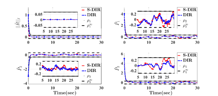
Refer to caption
Figure 3: Measured and true values of angular velocities.
Refer to caption
Figure 4: Measured and true values of translational velocities.
Refer to caption
Figure 5: True and measured body-frame vectorial measurements.
Refer to caption
Figure 6: True and estimated Euler angles of the rigid-body.
Refer to caption
Figure 7: True and estimated rigid-body positions in 3D space.
Refer to caption
Figure 8: Systematic convergence of the error trajectories within the prescribed performance boundaries.
Refer to caption
Figure 9: The estimated bias of the proposed filters.

The simulation results establish the strong filtering capability of the two proposed pose filters and their robustness against uncertain measurements and large initialized errors making them perfectly fit for the measurements obtained from low quality sensors such as IMU. The two filters conform to the dynamic constraints imposed by the user referring guaranteed prescribed performance measures in transient as well as steady-state performance. The pose filters previously proposed in the literature [12, 13, 16, 17, 18] lack this remarkable quality. Semi-direct pose filter with prescribed performance demands pose reconstruction, in this case attitude has been extracted using SVD [2, 3]. This adds complexity, and therefore the semi-direct pose filter requires more computational power in comparison with the direct pose filter with prescribed performance. Nevertheless, the two proposed pose filters are robust and demonstrate impressive convergence capabilities.

VI Conclusion

Two nonlinear pose filters evolved directly on 𝕊𝔼(3)𝕊𝔼3\mathbb{SE}\left(3\right) with prescribed performance characteristics have been considered. Pose error has been defined in terms of position error and normalized Euclidean distance error, and the innovation term has been selected to guarantee predefined measures of transient and steady-state performance. As a result, the proposed filters exhibit superior convergence properties with transient error being bounded by a predefined dynamically decreasing constrained function and steady-state error being less than a predefined lower bound. The proposed pose filters are deterministic and the stability analysis ensure boundedness of all closed loop signals with asymptotic convergence of the homogeneous transformation matrix to the origin. Simulation results established the strong ability of the proposed filters to impose the predefined constraints on the pose error considering large initial pose error and high level of uncertainties in the measurements.

Acknowledgment

The authors would like to thank Maria Shaposhnikova for proofreading the article.

Appendix A

Proof of Lemma 1

Let R𝕊𝕆(3)𝑅𝕊𝕆3R\in\mathbb{SO}\left(3\right) be the attitude of a rigid-body in 3D space. The attitude could be extracted for a given Rodriguez parameters vector ρ3𝜌superscript3\rho\in\mathbb{R}^{3}. The mapping from Rodriguez vector to 𝕊𝕆(3)𝕊𝕆3\mathbb{SO}\left(3\right) is defined by ρ:3𝕊𝕆(3):subscript𝜌superscript3𝕊𝕆3\mathcal{R}_{\rho}:\mathbb{R}^{3}\rightarrow\mathbb{SO}\left(3\right) [33]

ρ(ρ)=subscript𝜌𝜌absent\displaystyle\mathcal{R}_{\rho}\left(\rho\right)= 11+ρ2((1ρ2)𝐈3+2ρρ+2[ρ]×)11superscriptnorm𝜌21superscriptnorm𝜌2subscript𝐈32𝜌superscript𝜌top2subscriptdelimited-[]𝜌\displaystyle\frac{1}{1+||\rho||^{2}}\left(\left(1-||\rho||^{2}\right)\mathbf{I}_{3}+2\rho\rho^{\top}+2\left[\rho\right]_{\times}\right) (132)

With direct substitution of (132) in (4) one easily obtains [3]

RI=ρ21+ρ2subscriptnorm𝑅𝐼superscriptnorm𝜌21superscriptnorm𝜌2||R||_{I}=\frac{||\rho||^{2}}{1+||\rho||^{2}} (133)

Additionally, for ρ=ρ(ρ)subscript𝜌subscript𝜌𝜌\mathcal{R}_{\rho}=\mathcal{R}_{\rho}\left(\rho\right) the anti-symmetric projection operator of the attitude in (132) is equivalent to

𝓟a(R)=12(ρρ)=subscript𝓟𝑎𝑅12subscript𝜌superscriptsubscript𝜌topabsent\displaystyle\boldsymbol{\mathcal{P}}_{a}\left(R\right)=\frac{1}{2}\left(\mathcal{R}_{\rho}-\mathcal{R}_{\rho}^{\top}\right)= 211+ρ2[ρ]×211superscriptnorm𝜌2subscriptdelimited-[]𝜌\displaystyle 2\frac{1}{1+||\rho||^{2}}\left[\rho\right]_{\times} (134)

Thus, the vex operator of (134) becomes

𝐯𝐞𝐱(𝓟a(R))=2ρ1+ρ2𝐯𝐞𝐱subscript𝓟𝑎𝑅2𝜌1superscriptnorm𝜌2\mathbf{vex}\left(\boldsymbol{\mathcal{P}}_{a}\left(R\right)\right)=2\frac{\rho}{1+||\rho||^{2}} (135)

From the result in (133) one can obtain

(1RI)RI=ρ2(1+ρ2)21subscriptnorm𝑅𝐼subscriptnorm𝑅𝐼superscriptnorm𝜌2superscript1superscriptnorm𝜌22\left(1-||R||_{I}\right)||R||_{I}=\frac{||\rho||^{2}}{\left(1+||\rho||^{2}\right)^{2}} (136)

and from (135) it is easily shown that

𝐯𝐞𝐱(𝓟a(R))2=4ρ2(1+ρ2)2superscriptnorm𝐯𝐞𝐱subscript𝓟𝑎𝑅24superscriptnorm𝜌2superscript1superscriptnorm𝜌22||\mathbf{vex}\left(\boldsymbol{\mathcal{P}}_{a}\left(R\right)\right)||^{2}=4\frac{||\rho||^{2}}{\left(1+||\rho||^{2}\right)^{2}} (137)

Therefore, (136) and (137) prove (32) in Lemma 1. From Section IV-B i=1NRkiR=3superscriptsubscript𝑖1subscript𝑁Rsuperscriptsubscript𝑘𝑖R3\sum_{i=1}^{N_{{\rm R}}}k_{i}^{{\rm R}}=3 which indicates that Tr{𝐌R}=3Trsubscript𝐌R3{\rm Tr}\left\{\mathbf{M}_{{\rm R}}\right\}=3. Recall that the normalized Euclidean distance of R𝐌R𝑅subscript𝐌RR\mathbf{M}_{{\rm R}} is R𝐌RI=14Tr{(𝐈3R)𝐌R}subscriptnorm𝑅subscript𝐌R𝐼14Trsubscript𝐈3𝑅subscript𝐌R\left\|R\mathbf{M}_{{\rm R}}\right\|_{I}=\frac{1}{4}{\rm Tr}\left\{\left(\mathbf{I}_{3}-R\right)\mathbf{M}_{{\rm R}}\right\}. From the angle-axis parameterization in (5), one finds

R𝐌RIsubscriptnorm𝑅subscript𝐌R𝐼\displaystyle\left\|R\mathbf{M}_{{\rm R}}\right\|_{I} =14Tr{(sin(θ)[u]×+(1cos(θ))[u]×2)𝐌R}absent14Tr𝜃subscriptdelimited-[]𝑢1𝜃superscriptsubscriptdelimited-[]𝑢2subscript𝐌R\displaystyle=\frac{1}{4}{\rm Tr}\left\{-\left(\sin(\theta)\left[u\right]_{\times}+\left(1-\cos(\theta)\right)\left[u\right]_{\times}^{2}\right)\mathbf{M}_{{\rm R}}\right\}
=14Tr{(1cos(θ))[u]×2𝐌R}absent14Tr1𝜃superscriptsubscriptdelimited-[]𝑢2subscript𝐌R\displaystyle=-\frac{1}{4}{\rm Tr}\left\{\left(1-\cos(\theta)\right)\left[u\right]_{\times}^{2}\mathbf{M}_{{\rm R}}\right\} (138)

where Tr{[u]×𝐌R}=0Trsubscriptdelimited-[]𝑢subscript𝐌R0{\rm Tr}\left\{\left[u\right]_{\times}\mathbf{M}_{{\rm R}}\right\}=0 as in identity (10). One has [34]

RI=14Tr{𝐈3R}=sin2(θ/2)subscriptnorm𝑅𝐼14Trsubscript𝐈3𝑅superscriptsin2𝜃2\left\|R\right\|_{I}=\frac{1}{4}{\rm Tr}\left\{\mathbf{I}_{3}-R\right\}={\rm sin}^{2}\left(\theta/2\right) (139)

The Rodriguez vector can be expressed in terms of angle-axis parameterization as [33]

u=cot(θ/2)ρ𝑢cot𝜃2𝜌u={\rm cot}\left(\theta/2\right)\rho (140)

From identity (8) and (140), the expression in (138) becomes

R𝐌RIsubscriptnorm𝑅subscript𝐌R𝐼\displaystyle\left\|R\mathbf{M}_{{\rm R}}\right\|_{I} =12RIu𝐌¯Ru=12RIcot2(θ2)ρ𝐌¯Rρabsent12subscriptnorm𝑅𝐼superscript𝑢topsubscript¯𝐌R𝑢12subscriptnorm𝑅𝐼superscriptcot2𝜃2superscript𝜌topsubscript¯𝐌R𝜌\displaystyle=\frac{1}{2}\left\|R\right\|_{I}u^{\top}\bar{\mathbf{M}}_{{\rm R}}u=\frac{1}{2}\left\|R\right\|_{I}{\rm cot}^{2}\left(\frac{\theta}{2}\right)\rho^{\top}\bar{\mathbf{M}}_{{\rm R}}\rho

Also, from (139), cos2(θ2)=1RIsuperscriptcos2𝜃21subscriptnorm𝑅𝐼{\rm cos}^{2}\left(\frac{\theta}{2}\right)=1-\left\|R\right\|_{I} which implies that

tan2(θ2)=RI1RIsuperscripttan2𝜃2subscriptnorm𝑅𝐼1subscriptnorm𝑅𝐼{\rm tan}^{2}\left(\frac{\theta}{2}\right)=\frac{\left\|R\right\|_{I}}{1-\left\|R\right\|_{I}}

Accordingly, the normalized Euclidean distance of R𝐌R𝑅subscript𝐌RR\mathbf{M}_{{\rm R}} could be formulated in the sense of Rodriguez vector

R𝐌RIsubscriptnorm𝑅subscript𝐌R𝐼\displaystyle\left\|R\mathbf{M}_{{\rm R}}\right\|_{I} =12(1RI)ρ𝐌¯Rρ=12ρ𝐌¯Rρ1+ρ2absent121subscriptnorm𝑅𝐼superscript𝜌topsubscript¯𝐌R𝜌12superscript𝜌topsubscript¯𝐌R𝜌1superscriptnorm𝜌2\displaystyle=\frac{1}{2}\left(1-\left\|R\right\|_{I}\right)\rho^{\top}\bar{\mathbf{M}}_{{\rm R}}\rho=\frac{1}{2}\frac{\rho^{\top}\bar{\mathbf{M}}_{{\rm R}}\rho}{1+\left\|\rho\right\|^{2}} (141)

The anti-symmetric projection operator of R𝐌R𝑅subscript𝐌RR\mathbf{M}_{{\rm R}} can be defined in terms of Rodriquez vector using identity (6) and (9) by

𝓟a(R𝐌R)subscript𝓟𝑎𝑅subscript𝐌R\displaystyle\boldsymbol{\mathcal{P}}_{a}\left(R\mathbf{M}_{{\rm R}}\right) =ρρ𝐌R𝐌Rρρ+𝐌R[ρ]×+[ρ]×𝐌R1+ρ2absent𝜌superscript𝜌topsubscript𝐌Rsubscript𝐌R𝜌superscript𝜌topsubscript𝐌Rsubscriptdelimited-[]𝜌subscriptdelimited-[]𝜌subscript𝐌R1superscriptnorm𝜌2\displaystyle=\frac{\rho\rho^{\top}\mathbf{M}_{{\rm R}}-\mathbf{M}_{{\rm R}}\rho\rho^{\top}+\mathbf{M}_{{\rm R}}\left[\rho\right]_{\times}+\left[\rho\right]_{\times}\mathbf{M}_{{\rm R}}}{1+\left\|\rho\right\|^{2}}
=[(Tr{𝐌R}𝐈3𝐌R[ρ]×𝐌R)ρ]×1+ρ2absentsubscriptdelimited-[]Trsubscript𝐌Rsubscript𝐈3subscript𝐌Rsubscriptdelimited-[]𝜌subscript𝐌R𝜌1superscriptnorm𝜌2\displaystyle=\frac{\left[\left({\rm Tr}\left\{\mathbf{M}_{{\rm R}}\right\}\mathbf{I}_{3}-\mathbf{M}_{{\rm R}}-\left[\rho\right]_{\times}\mathbf{M}_{{\rm R}}\right)\rho\right]_{\times}}{1+\left\|\rho\right\|^{2}}

Thereby, the vex operator of the above expression is

𝐯𝐞𝐱(𝓟a(R𝐌R))𝐯𝐞𝐱subscript𝓟𝑎𝑅subscript𝐌R\displaystyle\mathcal{\mathbf{vex}}\left(\boldsymbol{\mathcal{P}}_{a}\left(R\mathbf{M}_{{\rm R}}\right)\right) =(𝐈3+[ρ]×)1+ρ2𝐌¯Rρabsentsubscript𝐈3subscriptdelimited-[]𝜌1superscriptnorm𝜌2subscript¯𝐌R𝜌\displaystyle=\frac{\left(\mathbf{I}_{3}+\left[\rho\right]_{\times}\right)}{1+\left\|\rho\right\|^{2}}\bar{\mathbf{M}}_{{\rm R}}\rho (142)

Hence, the 2-norm of (142) is equivalent to

𝐯𝐞𝐱(𝓟a(R𝐌R))2superscriptnorm𝐯𝐞𝐱subscript𝓟𝑎𝑅subscript𝐌R2\displaystyle\left\|\mathcal{\mathbf{vex}}\left(\boldsymbol{\mathcal{P}}_{a}\left(R\mathbf{M}_{{\rm R}}\right)\right)\right\|^{2} =ρ𝐌¯R(𝐈3[ρ]×2)𝐌¯Rρ(1+ρ2)2absentsuperscript𝜌topsubscript¯𝐌Rsubscript𝐈3superscriptsubscriptdelimited-[]𝜌2subscript¯𝐌R𝜌superscript1superscriptnorm𝜌22\displaystyle=\frac{\rho^{\top}\bar{\mathbf{M}}_{{\rm R}}\left(\mathbf{I}_{3}-\left[\rho\right]_{\times}^{2}\right)\bar{\mathbf{M}}_{{\rm R}}\rho}{\left(1+\left\|\rho\right\|^{2}\right)^{2}}

From the identity in (8), [ρ]×2=ρ2𝐈3+ρρsuperscriptsubscriptdelimited-[]𝜌2superscriptnorm𝜌2subscript𝐈3𝜌superscript𝜌top\left[\rho\right]_{\times}^{2}=-||\rho||^{2}\mathbf{I}_{3}+\rho\rho^{\top} such that

𝐯𝐞𝐱(𝓟a(R𝐌R))2superscriptnorm𝐯𝐞𝐱subscript𝓟𝑎𝑅subscript𝐌R2\displaystyle\left\|\mathcal{\mathbf{vex}}\left(\boldsymbol{\mathcal{P}}_{a}\left(R\mathbf{M}_{{\rm R}}\right)\right)\right\|^{2} =ρ𝐌¯R(𝐈3[ρ]×2)𝐌¯Rρ(1+ρ2)2absentsuperscript𝜌topsubscript¯𝐌Rsubscript𝐈3superscriptsubscriptdelimited-[]𝜌2subscript¯𝐌R𝜌superscript1superscriptnorm𝜌22\displaystyle=\frac{\rho^{\top}\bar{\mathbf{M}}_{{\rm R}}\left(\mathbf{I}_{3}-\left[\rho\right]_{\times}^{2}\right)\bar{\mathbf{M}}_{{\rm R}}\rho}{\left(1+\left\|\rho\right\|^{2}\right)^{2}}
=ρ(𝐌¯R)2ρ1+ρ2(ρ𝐌¯Rρ)2(1+ρ2)2absentsuperscript𝜌topsuperscriptsubscript¯𝐌R2𝜌1superscriptnorm𝜌2superscriptsuperscript𝜌topsubscript¯𝐌R𝜌2superscript1superscriptnorm𝜌22\displaystyle=\frac{\rho^{\top}\left(\bar{\mathbf{M}}_{{\rm R}}\right)^{2}\rho}{1+\left\|\rho\right\|^{2}}-\frac{\left(\rho^{\top}\bar{\mathbf{M}}_{{\rm R}}\rho\right)^{2}}{\left(1+\left\|\rho\right\|^{2}\right)^{2}}
λ¯(1ρ21+ρ2)ρ𝐌¯Rρ1+ρ2absent¯𝜆1superscriptnorm𝜌21superscriptnorm𝜌2superscript𝜌topsubscript¯𝐌R𝜌1superscriptnorm𝜌2\displaystyle\geq\underline{\lambda}\left(1-\frac{\left\|\rho\right\|^{2}}{1+\left\|\rho\right\|^{2}}\right)\frac{\rho^{\top}\bar{\mathbf{M}}_{{\rm R}}\rho}{1+||\rho||^{2}}
2λ¯(1RI)R𝐌RIabsent2¯𝜆1subscriptnorm𝑅𝐼subscriptnorm𝑅subscript𝐌R𝐼\displaystyle\geq 2\underline{\lambda}\left(1-\left\|R\right\|_{I}\right)\left\|R\mathbf{M}_{{\rm R}}\right\|_{I} (143)

where λ¯=λ¯(𝐌¯R)¯𝜆¯𝜆subscript¯𝐌R\underline{\lambda}=\underline{\lambda}\left(\bar{\mathbf{M}}_{{\rm R}}\right) is the minimum singular value of 𝐌¯Rsubscript¯𝐌R\bar{\mathbf{M}}_{{\rm R}} and RI=ρ2/(1+ρ2)subscriptnorm𝑅𝐼superscriptnorm𝜌21superscriptnorm𝜌2\left\|R\right\|_{I}=\left\|\rho\right\|^{2}/\left(1+\left\|\rho\right\|^{2}\right) as in (133). One can find

1RI1subscriptnorm𝑅𝐼\displaystyle 1-\left\|R\right\|_{I} =14(1+Tr{R𝐌R𝐌R1})absent141Tr𝑅subscript𝐌Rsuperscriptsubscript𝐌R1\displaystyle=\frac{1}{4}\left(1+{\rm Tr}\left\{R\mathbf{M}_{{\rm R}}\mathbf{M}_{{\rm R}}^{-1}\right\}\right) (144)

Hence, from (143) and (144) the following inequality holds

𝐯𝐞𝐱(𝓟a(R𝐌R))2superscriptnorm𝐯𝐞𝐱subscript𝓟𝑎𝑅subscript𝐌R2\displaystyle\left\|\mathcal{\mathbf{vex}}\left(\boldsymbol{\mathcal{P}}_{a}\left(R\mathbf{M}_{{\rm R}}\right)\right)\right\|^{2} λ¯2(1+Tr{R𝐌R𝐌R1})R𝐌RIabsent¯𝜆21Tr𝑅subscript𝐌Rsuperscriptsubscript𝐌R1subscriptnorm𝑅subscript𝐌R𝐼\displaystyle\geq\frac{\underline{\lambda}}{2}\left(1+{\rm Tr}\left\{R\mathbf{M}_{{\rm R}}\mathbf{M}_{{\rm R}}^{-1}\right\}\right)\left\|R\mathbf{M}_{{\rm R}}\right\|_{I}

This validates (33) and completes the proof of Lemma 1.

Appendix B

Quaternion Representation

Define Q=[q0,q]𝕊3𝑄superscriptsubscript𝑞0superscript𝑞toptopsuperscript𝕊3Q=[q_{0},q^{\top}]^{\top}\in\mathbb{S}^{3} as a unit-quaternion with q0subscript𝑞0q_{0}\in\mathbb{R} and q3𝑞superscript3q\in\mathbb{R}^{3} such that 𝕊3={Q4|Q=q02+qq=1}superscript𝕊3conditional-set𝑄superscript4norm𝑄superscriptsubscript𝑞02superscript𝑞top𝑞1\mathbb{S}^{3}=\{\left.Q\in\mathbb{R}^{4}\right|||Q||=\sqrt{q_{0}^{2}+q^{\top}q}=1\}. Q1=[q0q]𝕊3superscript𝑄1superscriptdelimited-[]subscript𝑞0superscript𝑞toptopsuperscript𝕊3Q^{-1}=[\begin{array}[]{cc}q_{0}&-q^{\top}\end{array}]^{\top}\in\mathbb{S}^{3} denotes the inverse of Q𝑄Q. Define direct-product\odot as a quaternion product where the quaternion multiplication of Q1=[q01q1]𝕊3subscript𝑄1superscriptdelimited-[]subscript𝑞01superscriptsubscript𝑞1toptopsuperscript𝕊3Q_{1}=[\begin{array}[]{cc}q_{01}&q_{1}^{\top}\end{array}]^{\top}\in\mathbb{S}^{3} and Q2=[q02q2]𝕊3subscript𝑄2superscriptdelimited-[]subscript𝑞02superscriptsubscript𝑞2toptopsuperscript𝕊3Q_{2}=[\begin{array}[]{cc}q_{02}&q_{2}^{\top}\end{array}]^{\top}\in\mathbb{S}^{3} is Q1Q2=[q01q02q1q2,q01q2+q02q1+[q1]×q2]direct-productsubscript𝑄1subscript𝑄2subscript𝑞01subscript𝑞02superscriptsubscript𝑞1topsubscript𝑞2subscript𝑞01subscript𝑞2subscript𝑞02subscript𝑞1subscriptdelimited-[]subscript𝑞1subscript𝑞2Q_{1}\odot Q_{2}=[q_{01}q_{02}-q_{1}^{\top}q_{2},q_{01}q_{2}+q_{02}q_{1}+[q_{1}]_{\times}q_{2}]. The mapping from unit-quaternion (𝕊3superscript𝕊3\mathbb{S}^{3}) to 𝕊𝕆(3)𝕊𝕆3\mathbb{SO}\left(3\right) is described by Q:𝕊3𝕊𝕆(3):subscript𝑄superscript𝕊3𝕊𝕆3\mathcal{R}_{Q}:\mathbb{S}^{3}\rightarrow\mathbb{SO}\left(3\right)

Qsubscript𝑄\displaystyle\mathcal{R}_{Q} =(q02q2)𝐈3+2qq+2q0[q]×𝕊𝕆(3)absentsuperscriptsubscript𝑞02superscriptnorm𝑞2subscript𝐈32𝑞superscript𝑞top2subscript𝑞0subscriptdelimited-[]𝑞𝕊𝕆3\displaystyle=(q_{0}^{2}-||q||^{2})\mathbf{I}_{3}+2qq^{\top}+2q_{0}\left[q\right]_{\times}\in\mathbb{SO}\left(3\right) (145)

The quaternion identity is described by QI=[1,0,0,0]subscript𝑄Isuperscript1000topQ_{{\rm I}}=[1,0,0,0]^{\top} with QI=𝐈3subscriptsubscript𝑄Isubscript𝐈3\mathcal{R}_{Q_{{\rm I}}}=\mathbf{I}_{3}. Define the estimate of Q=[q0,q]𝕊3𝑄superscriptsubscript𝑞0superscript𝑞toptopsuperscript𝕊3Q=[q_{0},q^{\top}]^{\top}\in\mathbb{S}^{3} as Q^=[q^0,q^]𝕊3^𝑄superscriptsubscript^𝑞0superscript^𝑞toptopsuperscript𝕊3\hat{Q}=[\hat{q}_{0},\hat{q}^{\top}]^{\top}\in\mathbb{S}^{3} with Q^=(q^02q^2)𝐈3+2q^q^+2q^0[q^]×subscript^𝑄superscriptsubscript^𝑞02superscriptnorm^𝑞2subscript𝐈32^𝑞superscript^𝑞top2subscript^𝑞0subscriptdelimited-[]^𝑞\mathcal{R}_{\hat{Q}}=(\hat{q}_{0}^{2}-||\hat{q}||^{2})\mathbf{I}_{3}+2\hat{q}\hat{q}^{\top}+2\hat{q}_{0}\left[\hat{q}\right]_{\times}, see the map in (145). For any x3𝑥superscript3x\in\mathbb{R}^{3} and Q𝕊3𝑄superscript𝕊3Q\in\mathbb{S}^{3}, define the map

x¯¯𝑥\displaystyle\overline{x} =[0,x]4absentsuperscript0superscript𝑥toptopsuperscript4\displaystyle=[0,x^{\top}]^{\top}\in\mathbb{R}^{4}
𝐘(Q1,x)¯¯𝐘superscript𝑄1𝑥\displaystyle\overline{\mathbf{Y}(Q^{-1},x)} =[0𝐘(Q1,x)]=Q1[0x]Qabsentdelimited-[]0𝐘superscript𝑄1𝑥direct-productsuperscript𝑄1delimited-[]0𝑥𝑄\displaystyle=\left[\begin{array}[]{c}0\\ \mathbf{Y}(Q^{-1},x)\end{array}\right]=Q^{-1}\odot\left[\begin{array}[]{c}0\\ x\end{array}\right]\odot Q
𝐘(Q,x)¯¯𝐘𝑄𝑥\displaystyle\overline{\mathbf{Y}(Q,x)} =[0𝐘(Q,x)]=Q[0x]Q1absentdelimited-[]0𝐘𝑄𝑥direct-product𝑄delimited-[]0𝑥superscript𝑄1\displaystyle=\left[\begin{array}[]{c}0\\ \mathbf{Y}(Q,x)\end{array}\right]=Q\odot\left[\begin{array}[]{c}0\\ x\end{array}\right]\odot Q^{-1}

The equivalent quaternion representation and complete implementation steps of the filter in (47), (48), (49), (50), (51), and (52) is:

{υi=𝐘(Q1,υi)Qy:Reconstructed by QUEST algorithmQ~=[q~0,q~]=Q^Qy1R~I=1q~02Py=1i=1NLkiLi=1NLsiL(vi(L)𝐘(Qy,vi(L)))P~=P^𝐘(Q~,Py)Γ=Ωmb^WQ^˙=12[0ΓΓ[Γ]×]Q^P^˙=𝐘(Q^,Vmb^VWV)b^˙Ω=γ𝚿RRq~0𝐘(Q^1,q~)+γ[𝐘(Q^1,P~P^)]×𝐘(Q^1,𝚿PP)b^˙V=γ𝐘(Q^1,𝚿PP)WΩ=4kw𝚿RR𝚲R/4q~0q~WV=𝐘(Q^1,kw𝚿PP+[P~P^]×WΩ𝚲PP~)casessuperscriptsubscript𝜐𝑖absent𝐘superscript𝑄1superscriptsubscript𝜐𝑖subscript𝑄𝑦:absentReconstructed by QUEST algorithm~𝑄absentsuperscriptsubscript~𝑞0superscript~𝑞toptopdirect-product^𝑄superscriptsubscript𝑄𝑦1subscriptnorm~𝑅𝐼absent1superscriptsubscript~𝑞02subscript𝑃𝑦absent1superscriptsubscript𝑖1subscript𝑁Lsuperscriptsubscript𝑘𝑖Lsuperscriptsubscript𝑖1subscript𝑁Lsuperscriptsubscript𝑠𝑖Lsuperscriptsubscriptv𝑖L𝐘subscript𝑄𝑦superscriptsubscriptv𝑖L~𝑃absent^𝑃𝐘~𝑄subscript𝑃𝑦ΓabsentsubscriptΩ𝑚^𝑏𝑊˙^𝑄absent12delimited-[]0superscriptΓtopΓsubscriptdelimited-[]Γ^𝑄˙^𝑃absent𝐘^𝑄subscript𝑉𝑚subscript^𝑏𝑉subscript𝑊𝑉subscript˙^𝑏Ωabsent𝛾subscript𝚿𝑅subscript𝑅subscript~𝑞0𝐘superscript^𝑄1~𝑞otherwise𝛾subscriptdelimited-[]𝐘superscript^𝑄1~𝑃^𝑃𝐘superscript^𝑄1subscript𝚿𝑃subscript𝑃subscript˙^𝑏𝑉absent𝛾𝐘superscript^𝑄1subscript𝚿𝑃subscript𝑃subscript𝑊Ωabsent4subscript𝑘𝑤subscript𝚿𝑅subscript𝑅subscript𝚲𝑅4subscript~𝑞0~𝑞subscript𝑊𝑉absent𝐘superscript^𝑄1subscript𝑘𝑤subscript𝚿𝑃subscript𝑃subscriptdelimited-[]~𝑃^𝑃subscript𝑊Ωsubscript𝚲𝑃~𝑃\begin{cases}\upsilon_{i}^{\mathcal{B}}&=\mathbf{Y}(Q^{-1},\upsilon_{i}^{\mathcal{I}})\\ Q_{y}&:\text{Reconstructed by QUEST algorithm}\\ \tilde{Q}&=[\tilde{q}_{0},\tilde{q}^{\top}]^{\top}=\hat{Q}\odot Q_{y}^{-1}\\ ||\tilde{R}||_{I}&=1-\tilde{q}_{0}^{2}\\ P_{y}&=\frac{1}{\sum_{i=1}^{N_{{\rm L}}}k_{i}^{{\rm L}}}\sum_{i=1}^{N_{{\rm L}}}s_{i}^{{\rm L}}\left({\rm v}_{i}^{\mathcal{I}\left({\rm L}\right)}-\mathbf{Y}\left(Q_{y},{\rm v}_{i}^{\mathcal{B}\left({\rm L}\right)}\right)\right)\\ \tilde{P}&=\hat{P}-\mathbf{Y}\left(\tilde{Q},P_{y}\right)\\ \Gamma&=\Omega_{m}-\hat{b}-W\\ \dot{\hat{Q}}&=\frac{1}{2}\left[\begin{array}[]{cc}0&-\Gamma^{\top}\\ \Gamma&-\left[\Gamma\right]_{\times}\end{array}\right]\hat{Q}\\ \dot{\hat{P}}&=\mathbf{Y}\left(\hat{Q},V_{m}-\hat{b}_{V}-W_{V}\right)\\ \dot{\hat{b}}_{\Omega}&=\gamma\boldsymbol{\Psi}_{R}\mathcal{E}_{R}\tilde{q}_{0}\mathbf{Y}\left(\hat{Q}^{-1},\tilde{q}\right)\\ &\hskip 10.00002pt+\gamma\left[\mathbf{Y}\left(\hat{Q}^{-1},\tilde{P}-\hat{P}\right)\right]_{\times}\mathbf{Y}\left(\hat{Q}^{-1},\boldsymbol{\Psi}_{P}\mathcal{E}_{P}\right)\\ \dot{\hat{b}}_{V}&=\gamma\mathbf{Y}\left(\hat{Q}^{-1},\boldsymbol{\Psi}_{P}\mathcal{E}_{P}\right)\\ W_{\Omega}&=4\frac{k_{w}\boldsymbol{\Psi}_{R}\mathcal{E}_{R}-\boldsymbol{\Lambda}_{R}/4}{\tilde{q}_{0}}\tilde{q}\\ W_{V}&=\mathbf{Y}\left(\hat{Q}^{-1},k_{w}\boldsymbol{\Psi}_{P}\mathcal{E}_{P}+\left[\tilde{P}-\hat{P}\right]_{\times}W_{\Omega}-\boldsymbol{\Lambda}_{P}\tilde{P}\right)\end{cases}

The equivalent quaternion representation and complete implementation steps of the filter in (114), (115), (116), (117), (118), and (119) is:

{[0υi]=[0𝐘(Q1,υi)]=Q1[0υi]Q[0υ^i]=[0𝐘(Q^1,υi)]=Q^1[0υi]Q^𝚼=𝐘(Q^,i=1NR(siR2υ^i(R)×υi(R)))R~𝐌RI=14i=1NR(1(υ^i(R))υi(R))M1=i=1NRsiRυi(R)(υi(R))M2=(i=1NRsiRυ^i(R)(υi(R)))1P~=P^+1𝐦c(𝐘(Q^,𝐤v)M1M2𝐦v)Γ=Ωmb^WQ^˙=12[0ΓΓ[Γ]×]Q^P^˙=𝐘(Q^,Vmb^VWV)b^˙Ω=γ2𝚿RR𝐘(Q^1,𝚼)+γ[𝐘(Q^1,P~P^)]×𝐘(Q^1,𝚿PP)b^˙V=γ𝐘(Q^1,𝚿PP)WΩ=4λ¯kw𝚿RR𝚲R1+Tr{M1M2}𝚼WV=𝐘(Q^1,kw𝚿PP+[P~P^]×WΩ𝚲PP~)casesdelimited-[]0superscriptsubscript𝜐𝑖absentdelimited-[]0𝐘superscript𝑄1superscriptsubscript𝜐𝑖direct-productsuperscript𝑄1delimited-[]0superscriptsubscript𝜐𝑖𝑄delimited-[]0superscriptsubscript^𝜐𝑖absentdelimited-[]0𝐘superscript^𝑄1superscriptsubscript𝜐𝑖direct-productsuperscript^𝑄1delimited-[]0superscriptsubscript𝜐𝑖^𝑄𝚼absent𝐘^𝑄superscriptsubscript𝑖1subscript𝑁Rsuperscriptsubscript𝑠𝑖R2superscriptsubscript^𝜐𝑖Rsuperscriptsubscript𝜐𝑖Rsubscriptnorm~𝑅subscript𝐌R𝐼absent14superscriptsubscript𝑖1subscript𝑁R1superscriptsuperscriptsubscript^𝜐𝑖Rtopsuperscriptsubscript𝜐𝑖Rsubscript𝑀1absentsuperscriptsubscript𝑖1subscript𝑁Rsuperscriptsubscript𝑠𝑖Rsuperscriptsubscript𝜐𝑖Rsuperscriptsuperscriptsubscript𝜐𝑖Rtopsubscript𝑀2absentsuperscriptsuperscriptsubscript𝑖1subscript𝑁Rsuperscriptsubscript𝑠𝑖Rsuperscriptsubscript^𝜐𝑖Rsuperscriptsuperscriptsubscript𝜐𝑖Rtop1~𝑃absent^𝑃1subscript𝐦c𝐘^𝑄subscript𝐤vsubscript𝑀1subscript𝑀2subscript𝐦vΓabsentsubscriptΩ𝑚^𝑏𝑊˙^𝑄absent12delimited-[]0superscriptΓtopΓsubscriptdelimited-[]Γ^𝑄˙^𝑃absent𝐘^𝑄subscript𝑉𝑚subscript^𝑏𝑉subscript𝑊𝑉subscript˙^𝑏Ωabsent𝛾2subscript𝚿𝑅subscript𝑅𝐘superscript^𝑄1𝚼otherwise𝛾subscriptdelimited-[]𝐘superscript^𝑄1~𝑃^𝑃𝐘superscript^𝑄1subscript𝚿𝑃subscript𝑃subscript˙^𝑏𝑉absent𝛾𝐘superscript^𝑄1subscript𝚿𝑃subscript𝑃subscript𝑊Ωabsent4¯𝜆subscript𝑘𝑤subscript𝚿𝑅subscript𝑅subscript𝚲𝑅1TrsubscriptM1subscriptM2𝚼subscript𝑊𝑉absent𝐘superscript^𝑄1subscript𝑘𝑤subscript𝚿𝑃subscript𝑃subscriptdelimited-[]~𝑃^𝑃subscript𝑊Ωsubscript𝚲𝑃~𝑃\begin{cases}\left[\begin{array}[]{c}0\\ \upsilon_{i}^{\mathcal{B}}\end{array}\right]&=\left[\begin{array}[]{c}0\\ \mathbf{Y}(Q^{-1},\upsilon_{i}^{\mathcal{I}})\end{array}\right]=Q^{-1}\odot\left[\begin{array}[]{c}0\\ \upsilon_{i}^{\mathcal{I}}\end{array}\right]\odot Q\\ \left[\begin{array}[]{c}0\\ \hat{\upsilon}_{i}^{\mathcal{B}}\end{array}\right]&=\left[\begin{array}[]{c}0\\ \mathbf{Y}(\hat{Q}^{-1},\upsilon_{i}^{\mathcal{I}})\end{array}\right]=\hat{Q}^{-1}\odot\left[\begin{array}[]{c}0\\ \upsilon_{i}^{\mathcal{I}}\end{array}\right]\odot\hat{Q}\\ \boldsymbol{\Upsilon}&=\mathbf{Y}\left(\hat{Q},\sum_{i=1}^{N_{{\rm R}}}\left(\frac{s_{i}^{{\rm R}}}{2}\hat{\upsilon}_{i}^{\mathcal{B}\left({\rm R}\right)}\times\upsilon_{i}^{\mathcal{B}\left({\rm R}\right)}\right)\right)\\ ||\tilde{R}\mathbf{M}_{{\rm R}}||_{I}&=\frac{1}{4}\sum_{i=1}^{N_{{\rm R}}}\left(1-\left(\hat{\upsilon}_{i}^{\mathcal{B}\left({\rm R}\right)}\right)^{\top}\upsilon_{i}^{\mathcal{B}\left({\rm R}\right)}\right)\\ M_{1}&=\sum_{i=1}^{N_{{\rm R}}}s_{i}^{{\rm R}}\upsilon_{i}^{\mathcal{B}\left({\rm R}\right)}\left(\upsilon_{i}^{\mathcal{I}\left({\rm R}\right)}\right)^{\top}\\ M_{2}&=\left(\sum_{i=1}^{N_{{\rm R}}}s_{i}^{{\rm R}}\hat{\upsilon}_{i}^{\mathcal{B}\left({\rm R}\right)}\left(\upsilon_{i}^{\mathcal{I}\left({\rm R}\right)}\right)^{\top}\right)^{-1}\\ \tilde{P}&=\hat{P}+\frac{1}{\mathbf{m}_{{\rm c}}}\left(\mathbf{Y}\left(\hat{Q},\mathbf{k}_{{\rm v}}\right)-M_{1}M_{2}\mathbf{m}_{{\rm v}}\right)\\ \Gamma&=\Omega_{m}-\hat{b}-W\\ \dot{\hat{Q}}&=\frac{1}{2}\left[\begin{array}[]{cc}0&-\Gamma^{\top}\\ \Gamma&-\left[\Gamma\right]_{\times}\end{array}\right]\hat{Q}\\ \dot{\hat{P}}&=\mathbf{Y}\left(\hat{Q},V_{m}-\hat{b}_{V}-W_{V}\right)\\ \dot{\hat{b}}_{\Omega}&=\frac{\gamma}{2}\boldsymbol{\Psi}_{R}\mathcal{E}_{R}\mathbf{Y}\left(\hat{Q}^{-1},\boldsymbol{\Upsilon}\right)\\ &\hskip 10.00002pt+\gamma\left[\mathbf{Y}\left(\hat{Q}^{-1},\tilde{P}-\hat{P}\right)\right]_{\times}\mathbf{Y}\left(\hat{Q}^{-1},\boldsymbol{\Psi}_{P}\mathcal{E}_{P}\right)\\ \dot{\hat{b}}_{V}&=\gamma\mathbf{Y}\left(\hat{Q}^{-1},\boldsymbol{\Psi}_{P}\mathcal{E}_{P}\right)\\ W_{\Omega}&=\frac{4}{\underline{\lambda}}\frac{k_{w}\boldsymbol{\Psi}_{R}\mathcal{E}_{R}-\boldsymbol{\Lambda}_{R}}{1+{\rm Tr\{M_{1}M_{2}\}}}\boldsymbol{\Upsilon}\\ W_{V}&=\mathbf{Y}\left(\hat{Q}^{-1},k_{w}\boldsymbol{\Psi}_{P}\mathcal{E}_{P}+\left[\tilde{P}-\hat{P}\right]_{\times}W_{\Omega}-\boldsymbol{\Lambda}_{P}\tilde{P}\right)\end{cases}

References

  • [1] M. D. Shuster and S. D. Oh, “Three-axis attitude determination from vector observations,” Journal of Guidance, Control, and Dynamics, vol. 4, pp. 70–77, 1981.
  • [2] F. L. Markley, “Attitude determination using vector observations and the singular value decomposition,” Journal of the Astronautical Sciences, vol. 36, no. 3, pp. 245–258, 1988.
  • [3] H. A. Hashim, L. J. Brown, and K. McIsaac, “Nonlinear stochastic attitude filters on the special orthogonal group 3: Ito and stratonovich,” IEEE Transactions on Systems, Man, and Cybernetics: Systems, pp. 1–13, 2018.
  • [4] R. Mahony, T. Hamel, and J.-M. Pflimlin, “Nonlinear complementary filters on the special orthogonal group,” IEEE Transactions on Automatic Control, vol. 53, no. 5, pp. 1203–1218, 2008.
  • [5] H. A. H. Mohamed, “Nonlinear attitude and pose filters with superior convergence properties,” Ph.D, University of Western Ontario, 2019.
  • [6] D. Choukroun, I. Y. Bar-Itzhack, and Y. Oshman, “Novel quaternion kalman filter,” IEEE Transactions on Aerospace and Electronic Systems, vol. 42, no. 1, pp. 174–190, 2006.
  • [7] E. J. Lefferts, F. L. Markley, and M. D. Shuster, “Kalman filtering for spacecraft attitude estimation,” Journal of Guidance, Control, and Dynamics, vol. 5, no. 5, pp. 417–429, 1982.
  • [8] F. L. Markley, “Attitude error representations for kalman filtering,” Journal of guidance, control, and dynamics, vol. 26, no. 2, pp. 311–317, 2003.
  • [9] H. A. Hashim, L. J. Brown, and K. McIsaac, “Nonlinear explicit stochastic attitude filter on SO(3),” in Proceedings of the 57th IEEE conference on Decision and Control (CDC).   IEEE, 2018, pp. 1210 –1216.
  • [10] H. F. Grip, T. I. Fossen, T. A. Johansen, and A. Saberi, “Attitude estimation using biased gyro and vector measurements with time-varying reference vectors,” IEEE Transactions on Automatic Control, vol. 57, no. 5, pp. 1332–1338, 2012.
  • [11] S. Q. Liu and R. Zhu, “A complementary filter based on multi-sample rotation vector for attitude estimation,” IEEE Sensors Journal, 2018.
  • [12] H. Rehbinder and B. K. Ghosh, “Pose estimation using line-based dynamic vision and inertial sensors,” IEEE Transactions on Automatic Control, vol. 48, no. 2, pp. 186–199, 2003.
  • [13] G. Baldwin, R. Mahony, J. Trumpf, T. Hamel, and T. Cheviron, “Complementary filter design on the special euclidean group se (3),” in Control Conference (ECC), 2007 European.   IEEE, 2007, pp. 3763–3770.
  • [14] H. A. Hashim, L. J. Brown, and K. McIsaac, “Nonlinear stochastic position and attitude filter on the special euclidean group 3,” Journal of the Franklin Institute, vol. 356, no. 7, pp. 4144–4173, 2018.
  • [15] H. A. Hashim, L. J. Brown, and K. McIsaac, “Guaranteed performance of nonlinear pose filter on SE(3),” in Proceedings of the American Control Conference (ACC), 2019, pp. 1–6.
  • [16] G. Baldwin, R. Mahony, and J. Trumpf, “A nonlinear observer for 6 dof pose estimation from inertial and bearing measurements,” in Robotics and Automation, 2009. ICRA’09. IEEE International Conference on.   IEEE, 2009, pp. 2237–2242.
  • [17] M.-D. Hua, T. Hamel, R. Mahony, and J. Trumpf, “Gradient-like observer design on the special euclidean group se (3) with system outputs on the real projective space,” in Decision and Control (CDC), 2015 IEEE 54th Annual Conference on.   IEEE, 2015, pp. 2139–2145.
  • [18] J. F. Vasconcelos, R. Cunha, C. Silvestre, and P. Oliveira, “A nonlinear position and attitude observer on se (3) using landmark measurements,” Systems & Control Letters, vol. 59, no. 3, pp. 155–166, 2010.
  • [19] S. Dominguez, “Simultaneous recognition and relative pose estimation of 3d objects using 4d orthonormal moments,” Sensors, vol. 17, no. 9, p. 2122, 2017.
  • [20] M.-D. Hua and G. Allibert, “Riccati observer design for pose, linear velocity and gravity direction estimation using landmark position and imu measurements,” in 2018 IEEE Conference on Control Technology and Applications, 2018.
  • [21] M. Tanaka, K. Tanaka, and H. O. Wang, “Practical model construction and stable control of an unmanned aerial vehicle with a parafoil-type wing,” IEEE Transactions on Systems, Man, and Cybernetics: Systems, 2017.
  • [22] F. Santoso, M. A. Garratt, S. G. Anavatti, and I. Petersen, “Robust hybrid nonlinear control systems for the dynamics of a quadcopter drone,” IEEE Transactions on Systems, Man, and Cybernetics: Systems, no. 99, pp. 1–13, 2018.
  • [23] L. Sun, W. Huo, and Z. Jiao, “Disturbance observer-based robust relative pose control for spacecraft rendezvous and proximity operations under input saturation,” IEEE Transactions on Aerospace and Electronic Systems, 2018.
  • [24] T. Lee, “Geometric control of quadrotor uavs transporting a cable-suspended rigid body,” IEEE Transactions on Control Systems Technology, vol. 26, no. 1, pp. 255–264, 2018.
  • [25] C. P. Bechlioulis and G. A. Rovithakis, “Robust adaptive control of feedback linearizable mimo nonlinear systems with prescribed performance,” IEEE Transactions on Automatic Control, vol. 53, no. 9, pp. 2090–2099, 2008.
  • [26] M. Wang and A. Yang, “Dynamic learning from adaptive neural control of robot manipulators with prescribed performance,” IEEE Transactions on Systems, Man, and Cybernetics: Systems, vol. 47, no. 8, pp. 2244–2255, 2017.
  • [27] Y. Yang, J. Tan, and D. Yue, “Prescribed performance tracking control of a class of uncertain pure-feedback nonlinear systems with input saturation,” IEEE Transactions on Systems, Man, and Cybernetics: Systems, 2018.
  • [28] J. Na, Q. Chen, X. Ren, and Y. Guo, “Adaptive prescribed performance motion control of servo mechanisms with friction compensation,” IEEE Transactions on Industrial Electronics, vol. 61, no. 1, pp. 486–494, 2014.
  • [29] H. A. Hashim, S. El-Ferik, and F. L. Lewis, “Neuro-adaptive cooperative tracking control with prescribed performance of unknown higher-order nonlinear multi-agent systems,” International Journal of Control, vol. 92, no. 2, pp. 445–460, 2019.
  • [30] H. A. Hashim, S. El-Ferik, and F. L. Lewis, “Adaptive synchronisation of unknown nonlinear networked systems with prescribed performance,” International Journal of Systems Science, vol. 48, no. 4, pp. 885–898, 2017.
  • [31] H. A. Hashim, L. J. Brown, and K. McIsaac, “Guaranteed performance of nonlinear attitude filters on the special orthogonal group SO(3),” IEEE Access, vol. 7, no. 1, pp. 3731–3745, 2019.
  • [32] F. Bullo and A. D. Lewis, Geometric control of mechanical systems: modeling, analysis, and design for simple mechanical control systems.   Springer Science & Business Media, 2004, vol. 49.
  • [33] M. D. Shuster, “A survey of attitude representations,” Navigation, vol. 8, no. 9, pp. 439–517, 1993.
  • [34] R. M. Murray, Z. Li, S. S. Sastry, and S. S. Sastry, A mathematical introduction to robotic manipulation.   CRC press, 1994.
[Uncaptioned image] Hashim A. Hashim (S’18) is a Ph.D. candidate in Robotics and Control, Department of Electrical and Computer Engineering at Western University, Ontario, Canada. He received the Bachelor’s degree in Mechatronics, Department of Mechanical Engineering from Helwan University, Cairo, Egypt and the M.Sc. in Systems and Control Engineering, Department of Systems Engineering from King Fahd University of Petroleum & Minerals, Dhahran, Saudi Arabia.
His current research interests include stochastic and deterministic attitude and pose filters, control of multi-agent systems, control applications and optimization techniques.
[Uncaptioned image] Lyndon J. Brown received the B.Sc. degree from the University of Waterloo, Canada in 1988 and the M.Sc. and PhD. degrees from the University of Illinois, Urbana-Champaign in 1991 and 1996, respectively. He is an associate professor in the department of electrical and computer engineering at Western University, Canada. He worked in industry for Honeywell Aerospace Canada and E.I. DuPont de Nemours.
His current research includes the identification and control of predictable signals, biological control systems, welding control systems, and attitude and pose estimation.
[Uncaptioned image] Kenneth McIsaac (M’99) received the B.Sc. degree from the University of Waterloo, Canada, in 1996, and the M.Sc. and Ph.D. degrees from the University of Pennsylvania, in 1998 and 2001, respectively. He is currently an Associate Professor and the Chair of Electrical and Computer Engineering with Western University, ON, Canada.
His current research interests include computer vision and signal processing, mostly in the context of using machine intelligence in robotics and assistive systems, and attitude and pose estimation.