Optimal Transport Relaxations
with Application to Wasserstein GANs

Abstract

We propose a family of relaxations of the optimal transport problem which regularize the problem by introducing an additional minimization step over a small region around one of the underlying transporting measures. The type of regularization that we obtain is related to smoothing techniques studied in the optimization literature. When using our approach to estimate optimal transport costs based on empirical measures, we obtain statistical learning bounds which are useful to guide the amount of regularization, while maintaining good generalization properties. To illustrate the computational advantages of our regularization approach, we apply our method to training Wasserstein GANs. We obtain running time improvements, relative to current benchmarks, with no deterioration in testing performance (via FID). The running time improvement occurs because our new optimality-based threshold criterion reduces the number of expensive iterates of the generating networks, while increasing the number of actor-critic iterations.

1 Introduction

Optimal transport costs, which include the Wasserstein Distance and the Earth-Mover-Distance as special cases, have become useful tools in machine learning and statistics [16, 3, 1, 18, 8, 6]. The optimal transport cost between two distributions is computed (in its primal form) as a minimization problem, in which the cost of transporting one distribution to another is minimized over all possible joint distributions, leading to linear program (see for example,[26]).

Optimal transport provides great flexibility when comparing (probability) measures and histograms. The transportation cost function (which we refer to as the cost function) can be used to capture key geometric characteristics [16]. It can be also used to compare discrete vs continuous distributions directly, without introducing smoothing, in contrast to alternatives such as the Kullback-Leibler divergence (see [3, 13] for more details). Also, by judiciously choosing the cost function, a Wasserstein distance can generate either the topology corresponding to weak convergence or the total variation distance.

In data-driven applications, one needs to estimate the optimal transport cost by means of sampled data. This involves using an empirical measure, say $\mu_{n}$, as a surrogates for the underlying population probability measure, say $\mu_{\infty}$. However, this direct approach fails to recognize that empirical measures are just imperfect descriptions of the underlying probabilities, and a small amount of perturbation in the empirical measure also may yield equally valid descriptions of the underlying probabilities. Adopting this perspective is particularly important in light of the fact that non-parametric empirical estimators of the Wasserstein distance converge slowly (at rate $O\left(n^{-1/d}\right))$ where $d$ is the underlying dimension of the distribution and $n$ the number of samples, see [9, 27]. It is natural to take the view that plausible variations of the data can be used to facilitate the estimation of optimal transport costs.

Using this insight, we provide a relaxation which regularizes the optimal transport cost between, $\mu_{n}$ and $\mu$, say $D_{\widetilde{c}}\left(\mu_{n},\mu\right)$ (depending on some cost function $\widetilde{c}\;$). Our relaxation takes the generic form

$$G_{\delta}\left(\mu_{n},\mu\right)=\inf\{D_{\widetilde{c}}\left(\nu,\mu\right):\nu\in\mathcal{D}_{\delta}\left(\mu_{n}\right)\},$$ (1)

where $\mathcal{D}_{\delta}\left(\mu_{n}\right)$ is a suitable region of ‘size’ $\delta$ around $\mu_{n}$. The region $\mathcal{D}_{\delta}\left(\mu_{n}\right)$ will typically be defined in terms of an optimal transport neighborhood of size $\delta$ around $\mu_{n}$, namely $\mathcal{D}_{\delta}\left(\mu_{n}\right)=\{\nu:D_{c}\left(\mu_{n},\nu\right)\leq\delta\}$, for some optimal transport cost $D_{c}\left(\mu_{n},\nu\right)$ depending on a cost function $c$. So, as $\delta\rightarrow 0$, we recover the standard optimal transport cost.

We stress that $\mathcal{D}_{\delta}\left(\mu_{n}\right)$ could be defined using criteria other than optimal transport, but given the flexibility mentioned earlier, we focus on optimal transport neighborhoods as stated earlier. We can also introduce a neighborhood around both $\mu_{n}$ and $\mu$ to define the inf. This modification can also be studied with the methods that we present.

The map $\mu_{n}\mapsto G_{\delta}\left(\mu_{n},\mu\right)$ is intuitively a more regular object than $G_{0}\left(\mu_{n},\mu\right)=D_{\widetilde{c}}\left(\mu_{n},\mu\right)$ as it is less sensitive to small perturbations of $\mu_{n}$. Of course, this type of regularity is also achieved by maximizing over a neighborhood of $\mu_{n}$ (instead of minimizing), but this operation leads to computational complications because the optimal transport cost is a convex functional. The dual formulation of the optimal transport costs can be used to connect our relaxation, at least formally, to smoothing techniques that are often used in the non-smooth convex optimization literature [22].

As indicated earlier, the regularization approach that we take is particularly meaningful given the slow rates of convergence in the empirical estimation of Wasserstein distances. Moreover, since the estimated Wasserstein distance is a positive random variable, the statistical error is likely to often have a right-tail bias, thus the minimization operation that we apply in (1) to regularize the Wasserstein distance is also sensible as a means of mitigating this bias. However, we need to be careful to not overcompensate. So, we also provide statistical learning bounds which can be used to ensure a choice of $\delta$ which enables the use of $G_{\delta}\left(\mu_{n},\mu\right)$, plus a small correction term, as an upper bound for $D_{\widetilde{c}}\left(\mu_{\infty},\mu\right)$. These statistical learning bounds are presented in Theorem 4. The parameter $\delta>0$ could also be chosen by a cross-validation procedure.

There are other regularization methods to estimate optimal transport costs. Some of these techniques require some smoothness or absolute continuity between the measures involved; this occurs, for example, when using entropic regularization, [8, 24, 14]. Others impose low rank constraints, as in [12], in the setting of domain adaptation, and others ([24, 14]) focus on specific applications such as Wasserstein GANs.

Our relaxation technique does not require smoothing or low rank properties. It acts directly at the same level of generality as the original optimal transport formulation. However, we are able to show that $G_{\delta}\left(\mu_{n},\mu\right)$ can often be evaluated directly and conveniently in terms of $D_{\widetilde{c}}\left(\mu_{n},\mu\right)$, leading to a variation of the optimal transport cost formulation which can then be used in conjunction with any of the regularization methods mentioned earlier. So, we do not see our work as a competitor to these regularization methods. Our approach can be reasonably viewed a pre-conditioning step which can be applied before any regularization tool that uses additional data structure.

As an application of our framework, we introduce a regularized Wasserstein GAN formulation which takes the form

$$\min_{\theta}\min_{\mathcal{W}\left(\mu_{n},\nu\right)\leq\delta}\mathcal{W}\left(\mu_{\theta},\nu\right)=\min_{\theta}G_{\delta}\left(\mu_{n},\mu_{\theta}\right)$$

where $\mathcal{W}\left(\mu_{\theta},\nu\right)$ is a Wasserstein distance between $\mu_{\theta}$ and $v$, and we are choosing $\widetilde{c}=c$, also coinciding with the metric used to define $\mathcal{W}$. The parameter $\theta$ represents the design of the generative network. The standard Wasserstein GAN formulation, [3], is recovered by setting $\delta=0$. In Section 2 we show that under mild assumptions,

$$\min_{\theta}\min_{\mathcal{W}\left(\mu_{n},\nu\right)\leq\delta}\mathcal{W}\left(\mu_{\theta},\nu\right)=\min_{\theta}\left(\mathcal{W}\left(\mu_{\theta},\mu_{n}\right)-\delta\right)^{+}.$$ (2)

Therefore, it is easily seen, after taking the gradients, that the number of iterates of the generative network, parameterized by $\theta$, is reduced relative to the actor-critic iterates, represented by $f$. While this implementation device (i.e. iterating the actor critic more often than the generator) is used in practice to speed up training times, our approach is theoretically supported from an optimality perspective. The inner minimization problem we introduce yields an optimal regularization form, which corresponds to ‘flattening’ the optimization surface in the parameter space $\theta$. The amount of flattening is governed by $\delta$, which should correspond to the degree of ambiguity in the data, measured from a statistical point of view. In summary, our Optimal Transport Relaxation (OTR) formulation suggests that training of the generative network can be reduced without loss of performance. We validate our findings by experimenting on two datasets: MNIST and CIFAR10.

Finally, we comment, owing to a duality result given in Theorem 1, that $G_{\delta}\left(\mu_{n},\mu_{\theta}\right)$ admits an economic interpretation as a distributionally robust revenue maximization problem in which an agent wishes to select a pricing policy which is robust to perturbations in a customer’s demand. While we do not exploit this interpretation directly in this paper, we believe that this formulation is of independent interest and thus it is worth exposing it in our Introduction.

The rest of the paper is organized as follows. In Section 2 we introduce the standard optimal transport problem, together with our novel OTR formulation. We compare the dual of the standard optimal transport problem to its robustified analogue. We show a strong duality result in the sense that the robustified optimal transport dual and primal achieve the same value. Next, using a general duality result in the distributionally robust optimization literature [6], we provide a convenient representation for the primal optimal transport problem. We use this representation to obtain closed form expressions for the contribution of the artificial player introduced in our distributionally robust formulation. These closed form expressions, in particular, include formulation (2). In Section 3, we discuss statistical learning bounds which provide generalization guarantees for our empirical estimator. We argue that our OTR-based estimator is intuitively more desirable than the standard empirical estimator for optimal transport costs, because it is directly seen to be smaller than the standard estimator. Nevertheless, Theorem 4 guarantees that it can be used to build an upper bound for the underlying optimal transport cost with high probability. We then provide numerical evidence to demonstrate our intuition. Our numerical examples suggest that our OTR estimator is often a better upper bound than the standard Wasserstein estimator. The proofs of all theorems are provided in the Appendix.

2 Problem Formulation, Interpretations and Tractability

We start by formulating the standard optimal transport problem. To do so, we shall introduce notation which will also be useful when describing our proposed formulation. Throughout the paper we will consider distributions supported on metric spaces $\mathcal{S}_{X}$ and $\mathcal{S}_{Y}$ with metrics $d_{X}$ and $d_{Y}$, respectively. We assume, for simplicity in the exposition that the spaces are complete, separable and compact.

We shall use $X$ to denote a generic random variables taking values in $\mathcal{S}_{X}$. Likewise, a generic random variable $Y$ will take values in $\mathcal{S}_{Y}$. The space of Borel probability measures defined on $\mathcal{S}_{X}$ and $\mathcal{S}_{Y}$ are defined as $\Pi_{X}$ and $\Pi_{Y}$, respectively. We use $\Pi_{X,Y}$ to denote the set of all couplings between $X,Y$ (i.e. joint Borel probability measures on $\mathcal{S}_{X}\times\mathcal{S}_{Y}$). Further, $\Pi_{X,Y}(\mu_{0},\nu)$ is the subset of $\Pi_{X,Y}$ such that $X\sim\mu_{0}$ and $Y\sim\nu$ (i.e. $X$ follows distribution $\mu$ and $Y$ follows distribution $\nu$).

Given a generic element $\pi\in\Pi_{X,Y}$, $\pi_{X}$ is the marginal distribution of $X$ and $\pi_{Y}$ is the marginal distribution of $Y$. So, $\pi\in\Pi_{X,Y}\left(\mu_{0},\nu\right)$ implies that $\pi_{X}=\mu_{0}$ and $\pi_{Y}=\nu$.

The standard optimal transport problem, also known as the Monge-Kantorovich problem, can be written as (see [26])

$$\mathcal{P}_{0}:D_{\widetilde{c}}\left(\mu_{0},\nu\right)=\min\{\mathbb{E}_{\pi}\widetilde{c}(X,Y):\pi\in\Pi_{X,Y}(\mu_{0},\nu)\}$$

where $\widetilde{c}:\mathcal{S}_{X}\times\mathcal{S}_{Y}\rightarrow[0,\infty)$ is a lower semi-continuous function. Clearly, $D_{\widetilde{c}}\left(\mu_{0},\nu\right)$ is the solution of a linear programming problem (albeit, an infinite dimensional one). We now consider the corresponding dual. First, let $C\left(\mathcal{S}_{X}\right)$ and $C\left(\mathcal{S}_{Y}\right)$ be the space of continuous functions on $\mathcal{S}_{X}$ and $\mathcal{S}_{Y}$, respectively. Next, define

$$\mathcal{A}\left(\widetilde{c}\right)=\{\left(\alpha,\beta\right)\in\mathcal{S}_{X}\times\mathcal{S}_{Y}:\alpha(x)+\beta(y)\leq\widetilde{c}(x,y)\text{ for all }x\in\mathcal{S}_{X},y\in\mathcal{S}_{Y}\},$$

then, the dual problem formulation of $\mathcal{P}_{0}$ is

$$\mathcal{\bar{P}}_{0}:\sup\{\mathbb{E}_{\mu_{0}}\alpha(X)+\mathbb{E}_{\nu}\beta(Y):\left(\alpha,\beta\right)\in\mathcal{A}\left(\widetilde{c}\right)\}.$$

It is known (see [26]) that strong duality holds.

To define our relaxed optimal transport formulation, we introduce the region

$$\mathcal{D}_{\delta}\left(\mu_{0}\right)=\{\nu:D_{c}\left(\mu_{0},\nu\right)\leq\delta\}.$$

We employ a lower semi-continuous cost function $c:\mathcal{S}_{X}\times\mathcal{S}_{X}\rightarrow[0,\infty)$ satisfying $c\left(x,x\right)=0$, so that $\mathcal{D}_{0}\left(\mu_{0}\right)=\{\mu_{0}\}$. As indicated in (1), we are interested in

$$G_{\delta}\left(\mu_{0},\nu\right)=\min\{D_{\widetilde{c}}\left(\mu,\nu\right):\mu\in\mathcal{D}_{\delta}\left(\mu_{0}\right)\}.$$

We have replaced the $\inf$ in (1) by $\min$ because $\mathcal{D}_{\delta}\left(\mu_{0}\right)$ is a compact set in the weak convergence topology (Prohorov’s theorem) and the optimal transport cost, as the supremum of linear and continuous functionals (by duality), is lower semicontinuous.

In terms of the dual problem $\mathcal{\bar{P}}_{0}$, our relaxed formulation then takes the form

$$G_{\delta}\left(\mu_{0},\nu\right)=\min_{\mu\in\mathcal{D}_{\delta}\left(\mu_{0}\right)}\sup_{\left(\alpha,\beta\right)\in\mathcal{A}\left(\widetilde{c}\right)}\mathbb{E}_{\mu}\alpha(X)+\mathbb{E}_{\nu}\beta(Y).$$

The next result indicates that duality holds in this representation, meaning, that $\min$ and $\sup$ can be exchanged, this will serve to provide useful interpretations for $G_{\delta}\left(\mu_{0},v\right)$.

Theorem 1.

$$G_{\delta}\left(\mu_{0},\nu\right)=\sup_{\left(\alpha,\beta\right)\in\mathcal{A}\left(\widetilde{c}\right)}\min_{\mu\in\mathcal{D}_{\delta}\left(\mu_{0}\right)}\mathbb{E}_{\mu}\alpha(X)+\mathbb{E}_{\nu}\beta(Y).$$

The above theorem can be used to provide a formal interpretation of our relaxation as a smoothing technique related to Nesterov’s smoothing [22]. We have

$$G_{\delta}\left(\mu_{0},v\right)=\sup_{-\alpha,\beta\in\mathcal{A}\left(\widetilde{c}\right)}\inf_{\mu\in\mathcal{D}_{\delta}\left(\mu_{0}\right)}E_{v}\beta\left(Y\right)-E_{\mu}\alpha\left(X\right)=\sup_{-\alpha,\beta\in\mathcal{A}\left(\widetilde{c}\right)}\left(E_{v}\beta\left(Y\right)-\phi\left(\alpha;\mu_{0}\right)\right)$$ (3)

where $\phi\left(\alpha;\mu_{0}\right)=\sup_{\mu\in\mathcal{D}_{\delta}\left(\mu_{0}\right)}E_{\mu}\alpha\left(X\right)$ is a convex function of $\alpha$. The above representation coincides in form with the smoothing operator technique introduced by Nesterov, see [22], equation (2.2). The resulting smooth mapping in Nesterov’s representation is to be considered as a function of $v$, namely $v\mapsto G_{\delta}\left(\mu_{0},v\right)$.

While we believe that it is interesting to study the transformation (3) in future research for the purpose of smoothing optimal transport problems, we shall focus on studying $G_{\delta}\left(\mu_{0},\nu\right)$. Note that controlling the size of $\delta$ will guarantee the validity of statistical bounds when estimating optimal transport costs from empirical data.

In addition to the smoothing interpretation given by (3), Theorem 1 also admits an economic interpretation. Consider an agent who offers a transportation service to two customers. One of them wishes to transport a pile of sand out of his/her backyard (this pile of sand is modeled according to distribution $\mu_{0}$, which represents the demand for the transportation service), while the other customer wishes to cover a sinkhole in his/her own backyard (the profile of the sinkhole is modeled by distribution $v$). It would cost $c\left(x,y\right)$ to transport mass from location $x$ to location $y$ if the customers arrange to solve this transportation problem among themselves. So, the agent would wish to charge a price $\alpha\left(x\right)$ per unit of mass transported from location $x$ to the first customer, a price $\beta\left(y\right)$ per unit of mass transported from location $y$ to the second customer, and would do so in such a way that it is cheaper to pay these prices than to pay the cost of transporting directly without the intervention of the agent, so $\alpha\left(x\right)+\beta\left(y\right)\leq c\left(x,y\right)$. But, of course, the agent wishes to maximize the total profit and this yields the dual interpretation for transporting items, encoded by distributions $\mu_{0},\nu$. Theorem 1 indicates that $G_{\delta}\left(\mu_{0},v\right)$ solves a distributionally robust revenue maximization problem, in which the agent selects a policy which is robust to perturbations in the shape of the pile of sand reported by the first customer.

Next, we provide another representation for $G_{\delta}(\mu_{0},\nu)$, which forms the basis for the design of gradient and subgradient algorithms and further simplifications.

Theorem 2.

$$G_{\delta}(\mu_{0},\nu)=(-1)\cdot\min_{\lambda\geq 0}\quad\left\{\lambda\delta+\max_{\pi\in\Pi_{W,Z}(\mu_{0},\nu)}\quad\mathbb{E}_{\pi}\left[h(W,Y,\lambda)\right]\right\}$$ (4)

where $h:\mathcal{S}_{X}\times\mathcal{S}_{Y}\times\mathbb{R}_{+}\rightarrow\mathbb{R}$ and $h(w,y,\lambda)=\sup_{x}\left\{-\widetilde{c}(x,y)-\lambda c(x,w)\right\}$.

The above result provides further insight into the smoothness properties introduced by our relaxation technique. For instance, min-max representation justifies understanding our relaxation as a regularization technique as in [10, 5]. Also, consider the case $\mathcal{S}_{X}=\mathcal{S}_{Y}$ and $c=d_{X}$. Then, the function $h(w,z,\lambda)$ becomes $\lambda$-Lipschitz in the $w$ argument. In particular, for all $w_{1},w_{2}\in\mathcal{S}_{X}$,

$$h(w_{1},z,\lambda)-h(w_{2},z,\lambda)\leq\sup_{x}\left\{\lambda c(x,w_{2})-\lambda c(x,w_{1})\right\}\leq\lambda d_{X}(w_{1},w_{2}).$$

So, Theorem 2 implies that solving for $G_{\delta}(\mu_{0},\nu)$ is equivalent to solving a standard optimal transport problem with measures $\mu_{0},\nu$ and a cost function that which replaces $\widetilde{c}(x,y)$ by a cost function which is $\lambda$-Lipschitz in $w$ and $\lambda$ is regularized.

In view of Theorem 2, we define

$$g(\lambda,\mu_{0},\nu)=\lambda\delta+\max_{\pi\in\Pi_{W,Y}(\mu_{0},\nu)}\quad\mathbb{E}_{\pi}\left[h(W,Y,\lambda)\right].$$

Thus, $G_{\delta}(\mu_{0},\nu)=-1\cdot\min_{\lambda\geq 0}\,g(\lambda,\mu_{0},\nu)$. The function $h(\cdot)$ is convex in $\lambda$ and subsequently $g(\cdot)$ is a convex function of $\lambda$. Hence, (4) is a convex optimization problem. Moreover, since $\lim_{\lambda\rightarrow\infty}g(\lambda,\mu_{0},\nu)=\infty$, the optimal solution set for (4) is bounded. Next, we provide a result which can be used as a basis for a subgradient algorithm to compute $G_{\delta}(\mu_{0},\nu)$.

Theorem 3.

If $\mathcal{S}_{X},\mathcal{S}_{Y}$ are convex subsets of $\mathbb{R}^{d}$ (for $d\in\mathbb{N}$), and $\widetilde{c},c$ are continuous, and $\widetilde{c}(\cdot,y)+\lambda c(\cdot,w)$ is a strictly convex function for $\lambda\geq 0,w$ and $y$, then $h$ is differentiable in $\lambda$, and the left-hand partial derivative of $g(\lambda,\mu_{0},\nu)$ with respect to $\lambda$ is

$$\delta+\min_{\pi\in\Pi^{\ast}({\lambda})}\mathbb{E}_{\pi}\left[\frac{\partial}{\partial\lambda}h(W,Y,\lambda)\right],$$

and the right-hand partial derivative of $g(\lambda,\mu_{0},\nu)$ with respect to $\lambda$ is

$$\delta+\max_{\pi\in\Pi^{\ast}({\lambda})}\mathbb{E}_{\pi}\left[\frac{\partial}{\partial\lambda}h(W,Y,\lambda)\right],$$

where $\Pi^{\ast}({\lambda})$ is set of optimal solutions to the problem

$$\max_{\pi}\quad\mathbb{E}_{\pi\in\Pi_{W,Y}(\mu_{0},\nu)}\left[h(W,Y,\lambda)\right]$$ (5)

Remark 1.

Theorem 3 still holds if the strict convexity condition for $\widetilde{c}(\cdot,y)+\lambda c(\cdot,w)$ is replaced with the condition that $\operatorname*{arg\,min}_{x\in\mathcal{S}_{X}}\{\widetilde{c}(x,y)+\lambda c(x,w)\}$ is a singleton for all $\lambda\geq 0,w$ and $y$.

Remark 2.

Function $g$ is differentiable at any point $\lambda$ if and only if the set $\{\mathbb{E}_{\pi}\left[\frac{\partial}{\partial\lambda}h(W,Y,\lambda)\right]|\;\pi\in\Pi^{\ast}({\lambda})\}$ is a singleton (for more details, see Corollary 4 of [21]).

Theorem 3 suggests implementing a subgradient method [4] to solve problem (4). In particular, at each iteration $t$, using $\lambda_{t-1}$, we can find $\pi_{\lambda_{t-1}}$ (a member of $\Pi^{\ast}({\lambda}_{t-1})$) and then $\lambda_{t}$. We assume we have access to an oracle to solve (5). Developing efficient methods to solve optimal transport problems as in (5) is a topic of separate interest which we will not focus in this paper. Once we arrive at the optimal solution $(\lambda^{*},\pi_{\lambda^{*}})$ (or a reasonable approximation of the optimal solution), then an optimal mapping between $y,x$ solving problem (4) can be constructed as follows.

1. For each point $y$, map it to a new point $w$ using $\pi_{\lambda^{*}}$.

2. Find $x$ as the solution to the problem $\sup_{x}\left\{-\widetilde{c}(x,y)-\lambda^{\ast}c(x,w)\right\}$.

We conclude this section with an example in which $G_{\delta}(\mu_{0},\nu)$ can be substantially simplified.

Example 1: Wasserstein Distances of Order 2

Let $\widetilde{c}(x,y)=||x-y||^{2}$ and $c(x,w)=||x-w||^{2}$. Then,

$$-G_{\delta}(\mu_{0},\nu)=\min_{\lambda\geq 0}\left\{\delta\lambda-\left(\frac{\lambda}{1+\lambda}\right)\cdot\left(\min_{\pi\in\Pi_{W,Y}(\mu_{0},\nu)}\mathbb{E}_{\pi}||W-Y||^{2}\right)\right\}$$

Let $H_{0}=\min_{\pi\in\Pi_{W,Y}(\mu_{0},\nu)}\mathbb{E}_{\pi}||W-Y||^{2}$. Then the optimal $\lambda$ is $\lambda=\left(\sqrt{\frac{H_{0}}{\delta}}-1\right)^{+}$.

Example 2: Wasserstein distance of order 1 and Wasserstein GANs

Let $\mathcal{S}_{X}=\mathcal{S}_{Y}$ with metric $d_{X}=d_{Y}=d$. For this subsection, let $\widetilde{c}(x,y)=c(x,y)=d(x,y)$ for all $x,y\in\mathcal{S}_{X}$.

First, we claim that

$$h(w,y,\lambda)=\begin{cases}-d(w,y),\quad\lambda>1\\ -\lambda d(w,y),\quad\lambda<1\end{cases}.$$

This can be seen as follows. Let $x_{(w,y)}=\operatorname*{arg\,max}_{x\in\mathcal{S}_{X}}\{\ -d(x,y)-\lambda d(x,w)\}$. Then for $\lambda>1$,

$$-d(w,y)=-d(w,y)-\lambda\cdot d(w,w)\leq-d(x_{(w,y)},y)-\lambda\cdot d(x_{(w,y)},w)$$

$$\Leftrightarrow \lambda\cdot d(x_{(w,y)},w)\leq d(w,y)-d(x_{(w,y)},y)\leq d(x_{(w,y)},w)$$

$$\Leftrightarrow (\lambda-1)d(x_{(w,y)},w)\leq 0\Leftrightarrow x_{(w,y)}=w.$$

A similar argument holds for $\lambda<1$.

In addition, since $h(w,y,\lambda)$ is the supremum of Lipschitz functions, it is continuous in $\lambda$. So, for $\lambda=1$, $h(w,y,\lambda)=-d(w,y)$. For $\lambda\geq 1$, the minimum of $g(\lambda,\mu_{0},\nu)$ occurs at $\lambda=1$. For $\lambda\in[0,1]$, if $G_{0}(\mu_{0},\nu)-\delta\leq 0$, the minimum of $g(\lambda,\mu_{0},\nu)$ occurs at $\lambda=0$; otherwise, the minimum occurs at $\lambda=1$. So,

$$G_{\delta}(\mu_{0},\nu)=\max\{G_{0}(\mu_{0},\nu)-\delta,0\}.$$ (6)

where $G_{0}(\mu_{0},\nu)$ is the order-1 Wasserstein distance between $\mu_{0},\nu$.

Expression (6) can be directly applied to training Wasserstein GANs. For additional background on these types of generative networks, see [3, 14]. Wasserstein GANs involve the optimization problem $\min_{\theta}G_{0}(\mu_{n},\mu_{\theta})$ where $\mu_{n}$ is the empirical measure of a real dataset and $\mu_{\theta}$ is a parametric probability measure to be constructed using a generative network.

Our OTR for Wasserstein GANs takes the form

$$\min_{\theta}G_{\delta}(\mu_{n},\mu_{\theta}) =\min_{\theta}\max\{G_{0}(\mu_{n},\mu_{\theta})-\delta,0\}$$

$$=\min_{\theta}\max\{\max_{f\in Lip\left(1\right)}E_{\mu_{n}}f\left(X\right)-E_{\mu_{\theta}}f\left(X\right)-\delta,0\}$$

$$=\min_{\theta}\max_{f\in Lip\left(1\right)}\left(E_{\mu_{n}}f\left(X\right)-E_{\mu_{\theta}}f\left(X\right)-\delta\right)^{+},$$ (7)

where $Lip\left(1\right)$ represent the space of 1-Lipschitz functions with respect to the metric $d\left(\cdot\right)$. Note that $\delta=0$ recovers the problem for Wasserstein GANs. Our implementation involves just a small modification of standard Wasserstein GAN platforms. However, it is important to choose the regularization parameter $\delta$ carefully. The next section provides statistical guidance to this effect.

Solving (7) requires only a simple augmentation to any stochastic gradient descent procedure proposed for Wasserstein GANs. In particular, (6) implies

$$\nabla_{\theta}G_{\delta}(\mu_{r},\mu_{\theta})=\nabla_{\theta}G_{0}(\mu_{r},\mu_{\theta})\mathbbm{1}\left(G_{0}(\mu_{r},\mu_{\theta})\geq\delta)\right)$$

where $\mathbbm{1}(\cdot)$ is the indicator function. So, in a stochastic gradient descent implementation, $\theta$ should be updated only when $\mathbbm{1}\left(G_{0}(\mu_{r},\mu_{\theta})\geq\delta)\right)$ and the procedure will be the same as for Wasserstein GANs. Experiment results are provided in Section 4.1.

3 The Statistics of the OTR Problem

In the previous section we studied the optimization problem $\min_{\lambda\geq 0}\,g(\lambda,\mu_{0},\nu)$ with respect to any distribution $\mu_{0}$. In this section, we study statistical guarantees when $\mu_{0}$ is given by an empirical measure $\mu_{n}$ of i.i.d. observations, so its canonical representation takes the form $\mu_{n}\left(dx\right)=n^{-1}\sum_{j=1}^{n}\delta_{X_{i}}\left(dx\right),$ with the $X_{i}$’s being i.i.d. copies of some distribution $\mu_{\infty}$. We derive a confidence interval for $G_{0}(\mu_{0},\nu)$ through the use of concentration inequalities.

In this section, we focus on the case where $\mathcal{S}_{X}=\mathcal{S}_{Y}$ and $d_{X}=d_{Y}$. In addition, for all $x,y\in\mathcal{S}_{X}$, we set $c(x,y)=d^{k}(x,y)$ where $k\geq 1$.

Suppose $c,\widetilde{c}$ are Lipschitz functions with Lipschitz constants $L(c)$ and $L(\widetilde{c})$ respectively. As a result, $h(w,y,\lambda)$ is Lipschitz in $(w,y)$ with Lipschitz constant $K_{\lambda}=O(L(c)\lambda\vee L(\widetilde{c}))$.

Define

$$\epsilon(n,\rho,\zeta,K_{\lambda}):= \sqrt{\frac{\log(\frac{1}{\rho})}{2n}}+4\zeta K_{\lambda}+$$

$$\frac{8\sqrt{2}K_{\lambda}}{\sqrt{n}}\int_{\zeta/4}^{4diam(\mathcal{S}_{X})}\sqrt{\mathcal{N}(\mathcal{S}_{X},d_{X},\xi/4)\log\left(2\left\lceil\frac{2diam(\mathcal{S}_{X})}{\xi}\right\rceil+1\right)}d{\xi}$$

where $\mathcal{N}(\mathcal{S}_{X},d_{X},\xi)$ is the $\xi$-covering number for ($\mathcal{S}_{X},d_{X}$).

Theorem 4.

For $k=1,d\geq 2,\zeta>0,\delta\geq 0,\lambda>L(\widetilde{c})$ with probability at least $1-\rho$,

$$G_{0}(\mu_{\infty},\nu)\leq G_{\delta}(\mu_{n},\nu)+\epsilon(n,\rho,\zeta,K_{\lambda})+\lambda\delta$$

Also for $k>1,d\geq 2,\zeta>0,\delta>0,\lambda=\delta^{-\frac{k-1}{k}}$ with probability at least $1-\rho$,

$$G_{0}(\mu_{\infty},\nu)\leq G_{\delta}(\mu_{n},\nu)+\epsilon(n,\rho,\zeta,K_{\lambda})+\left(2\cdot L^{\frac{k}{k-1}}(\widetilde{c})+1\right)\delta^{\frac{1}{k}}$$

Remark 3.

Theorem 4 also holds when $\mu_{n}$ and $\mu_{\infty}$ are switched. As a result, we obtain a confidence interval for $G_{0}(\mu_{\infty},\nu)$. In particular, with probability at least $1-2\rho$, $G_{0}(\mu_{\infty},\nu)$ resides in an interval centered at $G_{\delta}(\mu_{n},\nu)$ with radius $\epsilon(n,\rho,\zeta,K_{\lambda})+\lambda\delta$ for $k=1$ and radius $\epsilon(n,\rho,\zeta,K_{\lambda})+\left(2\cdot L^{\frac{k}{k-1}}(\widetilde{c})+1\right)\delta^{\frac{1}{k}}$ for $k>1$.

Remark 4.

By optimizing the upper bound in Theorem 4, we were able to recover the term $\frac{1}{n^{1/d}}$ (curse of dimensionality) [9]. For more details, see the appendix for Theorem 4.

4 Experiments

4.1 OTR Wasserstein GAN

This section provides experiment results evaluating OTR Wasserstein GANs (WGANs) in Section 2.

We trained on two dataset: MNIST [19] and CIFAR10 [17]. For the GAN implementation, we used the code provided by [14] and for Frechet Inception Distance (FID) calculation we used the code provided by [15]. For every fixed initial weights (seed), we trained our proposed GAN with different values of $\delta$. We performed training for 20000 generator iterations. For CIFAR10, $\delta\in\{0,1.9,2.0,2.1\}$. For MNIST, $\delta\in\{0,0.2,0.3,0.4\}$.

Representative results are provided in Figures 1,2 in log-log scale. Additional results that use different initializations are provided in the Appendix. Our experiments indicate that with an ‘appropriate’ choice of $\delta$, OTR WGAN has a similar test loss performance to WGAN. Also on the CIFAR10 dataset, they have similar Inception Score [23] performance. Moreover, OTR WGAN has either the same or faster FID[15] convergence rate than WGAN. In addition, OTR WGAN trains faster than WGAN because it skips training the Generator when the threshold criteria is not met. The ‘appropriate’ values for $\delta$ were found using cross validation. This ‘appropriate’ value for $\delta$ should be slightly greater than $\min_{\theta}\mathcal{W}(\mu_{n},\mu_{\theta})$. For values of $\delta$ considerably larger than $\min_{\theta}\mathcal{W}(\mu_{n},\mu_{\theta})$, training of OTR WGAN is faster; however, the FID performance of OTR WGAN is worse than WGAN. On the other hand for values of $\delta$ considerably less than $\min_{\theta}\mathcal{W}(\mu_{n},\mu_{\theta})$, the thresholding becomes ineffective and OTR WGAN behaves similar to WGAN. In addition, trying many different initial points (seeds) indicate that OTR WGAN is more stable and has less volatility compared to WGAN.

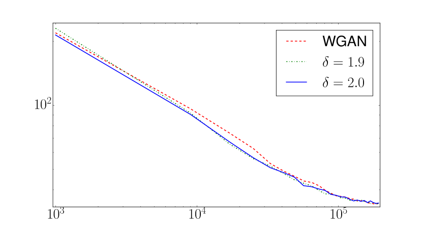
(a)

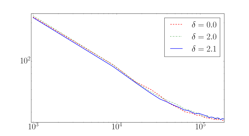
(b)

Figure 1: FID versus generator iteration on CIFAR10 for comparison of OTR WGAN and WGAN. Each subfigure presents a different initialization. In the legend, $\delta$ is the OTR WGAN parameter.

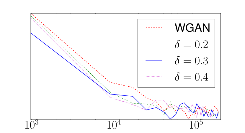
(a)

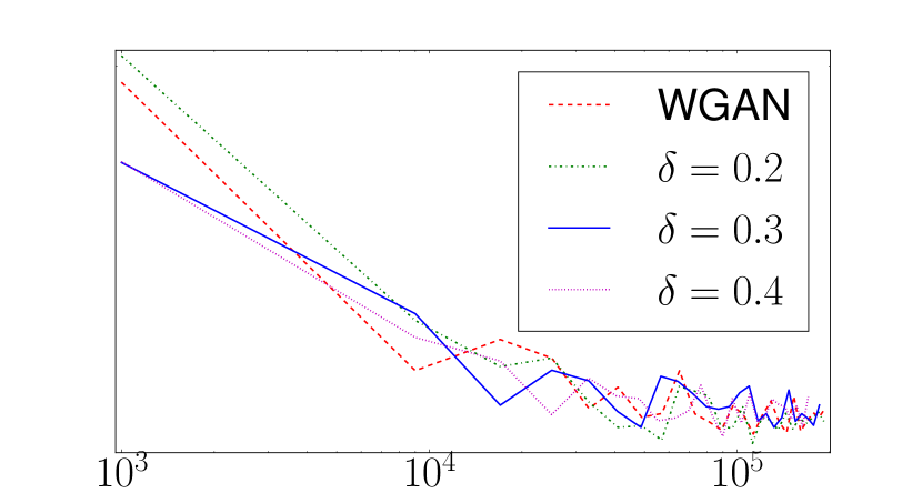
(b)

Figure 2: FID versus generator iteration on MNIST for comparison of OTR WGAN and WGAN. Each subfigure presents a different initialization. In the legend, $\delta$ is the OTR WGAN parameter.

4.2 Estimating the Optimal Transport Cost

In this section, we present simulation results denoting the value of optimal transport relaxation for estimating the Wasserstein distance between measures.

Let $\mu_{0},\nu$ be two probability measures defined on $\mathbb{R}^{20}$. The measure $\nu$ is constructed from $300$ i.i.d samples of $\mathcal{N}\left(0,I_{20\times 20}\right)$ where $I_{20\times 20}$ is the identity matrix. The measure $\mu_{0}$ is also constructed from $300$ i.i.d. sampling of a random vector $X\in\mathbb{R}^{20}$ defined as follows. For each component $X_{i}$ of $X$ ($1\leq i\leq 20$), $X_{i}:=\rho R_{i}+(1-\rho^{2})^{\frac{1}{2}}T$ where $\{R_{i}\}_{i=1}^{20},T$ are i.i.d. and $\mathcal{N}\left(0,1\right)$. In particular, $0\leq\rho\leq 1$ specifies dependence of the $X_{i}$’s.

For $n\in\mathbb{N}$, let $\hat{\mu}_{n}$ be an empirical probability measure constructed from $n$ i.i.d. samples from $\mu_{0}$. For $\widetilde{c}=c=\|\cdot\|^{2}_{2}$, we compute the values of $G_{\delta_{n}}(\hat{\mu}_{n},\nu),G_{0}(\hat{\mu}_{n},\nu)$ where $\delta_{n}=\frac{1}{n^{0.45}}$. Then we compare them with the value of $G_{0}({\mu}_{0},\nu)$. To solve the optimal transport problems, the implementation from the Python Optimal Transport Library [11] was used.

Our experiments indicate for large enough values of $n$, the empirical cost functions $G_{0}(\hat{\mu}_{n},\nu),G_{\delta_{n}}(\hat{\mu}_{n},\nu)$ often incur upward shifts relative to $G_{0}({\mu}_{0},\nu)$. This is illustrated in 3. Figure 3(a) and Figure 3(b) correspond to high and low dependence of the $X_{i}$’s, respectively.

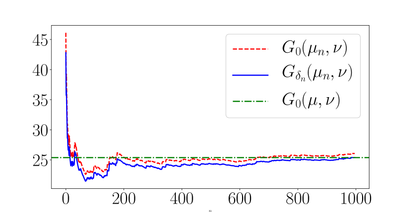
(a) $\rho=0.3$

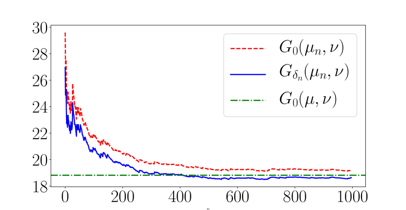
(b) $\rho=0.8$

Figure 3: Estimating the Optimal Transport Cost

Appendix A Proof of Theorem 1

The result follows directly from Sion’s min-max theorem (see [25]). First, the set $\mathcal{D}_{\delta}\left(\mu_{0}\right)$ is convex because, by duality, $D_{c}\left(\mu_{0},\cdot\right)$ is convex (because since it is the supremum of linear functionals). Next, since the spaces involved are compact, the set $\mathcal{D}_{\delta}\left(\mu_{0}\right)$ is compact in the weak convergence topology, by Prohorov’s theorem. Furthermore, it is immediate that the set $\mathcal{A}\left(\widetilde{c}\right)$ is convex. Finally, the objective function is bilinear both in $\left(\mu,v\right)$, on one hand, and $\left(\alpha,\beta\right)$ on the other. By definition of weak convergence, the functional is continuous in the weak convergence topology since the elements in $\mathcal{A}\left(\widetilde{c}\right)$ are both continuous, and bounded and the spaces are compact.

Appendix B Proof of Theorem 2

We have

$$G_{\delta}(\mu_{0},\nu)=\min_{D_{c}(\mu,\mu_{0})\leq\delta}\quad\min_{\pi\in\Pi_{X,Y}(\mu,\nu)}\quad\mathbb{E}_{\pi}\widetilde{c}(X,Y).$$

Given a coupling $\pi\in\Pi_{X,Y}(\mu,\nu)$ we can always have a coupling between $X$ and $W\sim\mu_{0}$ (by the gluing lemma, see [26]). Therefore, we have that

$$G_{\delta}(\mu_{0},\nu)=\min_{\pi}\quad \int\widetilde{c}(x,y)\pi(dx,dy,dw)$$

s.t. $$\int c(x,w)\pi(dx,dw)\leq\delta$$

$$\pi_{W}=\mu_{0},\pi_{Y}=\nu$$

which is the same as

$$-G_{\delta}(\mu_{0},\nu)=\max_{\pi}\quad \int-\widetilde{c}(x,y)\pi(dx,dy,dw)$$

s.t. $$\int c(x,w)\pi(dx,dw)\leq\delta$$

$$\pi_{W}=\mu_{0},\pi_{Y}=\nu$$

As a result,

$$-G_{\delta}(\mu_{0},\nu)=$$

$$\max_{\pi}\min_{\lambda\geq 0,h_{1}\in C\left(\mathcal{S}_{X}\right),h_{2}\in C\left(\mathcal{S}_{Y}\right)}\left[\int-\widetilde{c}(x,y)\pi(dx,dy,dw)+\int h_{1}(w)\mu_{0}(dw)-\right.$$

$$\left.\int h_{1}(w)\pi(dx,dy,dw)+\int h_{2}(y)\nu(dy)-\int h_{2}(y)\pi(dx,dy,dw)+\right.$$

$$\left.\lambda\left(\delta-\int c(x,w)\pi(dx,dw)\right)\right],$$

Further, Sion’s min-max Theorem [25] is applicable because the value function is both linear in $\pi$ and $(h_{1},h_{2})$. In particular, it is concave in $\pi$ and convex in $(h_{1},h_{2})$. We then need to argue upper semi-continuity as function of $\pi$ and lower semicontinuity as a function of $(h_{1},h_{2})$. We choose the topology of uniform convergence over the compact sets $\mathcal{S}_{X}$ and $\mathcal{S}_{Y}$. Continuity then follows easily by Dominated Convergence. Now, to show upper semicontinuity as a function of $\pi$, we consider the space of probabilities under the weak convergence topology. It suffices to show that $\int\widetilde{c}(x,y)\pi(dx,dy,dw)$ and $\int c(x,w)\pi(dx,dw)$ are lower semicontinuous as a function of $\pi$, since the remaining terms involving $\pi$ involve integrals of continuous functions over compact sets (hence continuous and bounded functions) and therefore those remaining terms are directly seen to be continuous by the definition of weak convergence (denoted by $\Rightarrow$). We need to show that if $\pi_{n}\Rightarrow\pi$ as $n\to\infty$, then $\liminf\int cd\pi_{n}\geq\int cd\pi$. By the Skorokhod representation, we may assume that there exists $Z_{n}=(X_{n},Y_{n},W_{n})$ such that $Z_{n}$ has distribution $\pi_{n}$ and $Z$ having distribution $\pi$, such that $Z_{n}\rightarrow Z$ almost surely as $n\to\infty$. Then, we have that

$$\liminf\int cd\pi_{n}=\liminf E(c(Z_{n}))\geq\int E(\liminf c(Z_{n}))\geq E(c(Z))=\int c\;d\pi,$$

where the first inequality follows by Fatou’s lemma and the second inequality follows because $c$ is lower semicontinuous. A similar argument holds for $\widetilde{c}$. As a result,

$$-G_{\delta}(\mu_{0},\nu)=$$

$$\min_{\lambda\geq 0,h_{1}\in C\left(\mathcal{S}_{X}\right),h_{2}\in C\left(\mathcal{S}_{Y}\right)}\max_{\pi}\left[\int\left(-\widetilde{c}(x,y)-h_{1}(w)-h_{2}(y)-\lambda c(x,w)\right)\pi(dx,dy,dw)\right.$$

$$\left.+\lambda\delta+\int h_{1}(w)\mu_{0}(dw)+\int h_{2}(y)\nu(dy)\right].$$

The above expression implies that for all $x,y,w$ we must have:

$$-\widetilde{c}(x,y)-h_{1}(w)-h_{2}(y)-\lambda c(x,w)\leq 0\Rightarrow\sup_{x}[-\widetilde{c}(x,y)-\lambda c(x,w)]\leq h_{1}(w)+h_{2}(y)$$

Therefore,

$$-G_{\delta}(\mu_{0},\nu) =\min_{\lambda\geq 0}\max_{\pi\in\Pi_{W,Y}(\mu_{0},\nu)}\left\{\lambda\delta+\mathbb{E}_{\mu_{0}}h_{1}(W)+\mathbb{E}_{\nu}h_{2}(Y)\right\}$$

$$=\min_{\lambda\geq 0}\max_{\pi\in\Pi_{W,Y}(\mu_{0},\nu)}\left\{\lambda\delta+\mathbb{E}_{\pi}\left[\sup_{x}\{-\widetilde{c}(x,Y)-\lambda c(x,W)\}\right]\right\}$$

$$=\min_{\lambda\geq 0}\left\{\lambda\delta+\max_{\pi\in\Pi_{W,Y}(\mu_{0},\nu)}\quad\mathbb{E}_{\pi}\left[\sup_{x}\left\{-\widetilde{c}(x,Y)-\lambda c(x,W)\right\}\right]\right\}$$

Appendix C Proof of Theorem 3

The differentiability of $h(\cdot)$ in $\lambda$ is an immediate result of Corollary 4 of [21].

Define

$$u(\lambda,\mu_{0},\nu)=\max_{\pi\in\Pi_{W,Y}(\mu_{0},\nu)}\quad \mathbb{E}_{\pi}\left[h(W,Y,\lambda)\right]$$

Therefore, $g(\lambda,\mu_{0},\nu)=\delta\lambda+u(\lambda,\mu_{0},\nu)$. In addition, define $f(\pi,\lambda)=\mathbb{E}_{\pi}\left[h(W,Y,\lambda)\right]$.

We need to show $\frac{\partial}{\partial\lambda}u(\lambda,\mu_{0},\nu)=\mathbb{E}_{\pi_{\lambda}^{*}}\left[\frac{\partial}{\partial\lambda}h(W,Y,\lambda)\right]$. For this statement to hold, according to Corollary 4 of [21], a sufficient condition is as follows. The set $\Pi(\mu_{0},\nu)$ needs to be compact, $f(\pi,\lambda)$ needs to be continuous in $\pi$, and $\frac{\partial}{\partial\lambda}f(\pi,\lambda)$ needs to be continuous in $(\pi,\lambda)$. In the remainder of this proof, we will show that this sufficient condition holds.

The set $\mathcal{S}_{X}\times\mathcal{S}_{Y}$ is compact. Therefore, Prohorov theorem implies under the weak convergence topology, $\Pi(\mu_{0},\nu)$ is a compact set.

On the other hand, the function $-\widetilde{c}(x,y)-\lambda c(x,w)$ is continuous in $(x,w,y,\lambda)$ and the supremum $\sup_{x}\left\{-\widetilde{c}(x,y)-\lambda c(x,w)\right\}$ is attained due to the compactness of $\mathcal{S}_{X},\mathcal{S}_{Y}$. Define $x^{*}(w,y,\lambda)$ to be the maximizing $x$, which will be unique (because $\widetilde{c}(\cdot,y)+\lambda c(\cdot,w)$ is strictly convex). Hence,

$$\sup_{x}\left\{-\widetilde{c}(x,y)-\lambda c(x,w)\right\}=-\widetilde{c}(x^{*}(w,y,\lambda),y)-\lambda c(x^{*}(w,y,\lambda),w)$$

Then, Berge’s maximum theorem [2] implies $h(w,y,\lambda)$ is continuous in $(w,y,\lambda)$ and $x^{*}(w,y,\lambda)$ is upper hemicontinuous in $(w,y,\lambda)$. Moreover, since $x^{*}$ is a single valued correspondence, it is continuous in $(w,y,\lambda)$.

Since it is defined on a compact set and continuous, $h(\cdot,\cdot,\lambda)$ is bounded. Also, $f(\cdot,\lambda)$ is linear in $\pi$. Therefore, under the weak convergence topology, $f(\pi,\lambda)$ is continuous in $\pi$.

Moreover,

$$\frac{\partial}{\partial\lambda}f(\pi,\lambda)$$

$$\overset{(a)}{=}\, \mathbb{E}_{\pi}\left[\frac{\partial}{\partial\lambda}h(W,Y,\lambda)\right]$$

$$=\, \mathbb{E}_{\pi}\left[-c(x^{*}(W,Y,\lambda),W)\right]$$ (8)

In the above statement, $(a)$ is an immediate result of the fact that $h(\cdot)$ is convex in $\lambda$ and the monotone convergence theorem together with the fact that $h(\cdot)$ is differentiable in $\lambda$. Since $c,x^{*}$ are continuous, the function $-c(x^{*}(W,Y,\lambda),W)$ is continuous in $(W,Y,\lambda)$. For fixed $\lambda$, this function is bounded since it is defined on a compact set. Thus the bounded convergence theorem implies (8) is continuous in $\lambda$. In addition, $\frac{\partial}{\partial\lambda}f(\pi,\lambda)$ is continuous in $\pi$ under the weak convergence topology. So, $\frac{\partial}{\partial\lambda}f(\pi,\lambda)$ is continuous in $(\pi,\lambda)$.

Appendix D Proof of Theorem 4 and Additional Comments

D.1 Proof of Theorem 4

It can be shown [26] that

$$f(X_{1},\cdots,X_{n}):=\min_{\pi\in\Pi_{W,Y}(\mu_{n},\nu)}\mathbb{E}_{\pi}\left\{-h(W,Y,\lambda)\right\}=\sup_{\alpha(\cdot)\in Lip(K_{\lambda})}\{\mathbb{E}_{\mu_{n}}\alpha(W)+\mathbb{E}_{\nu}\alpha_{\lambda}^{h}(Y)\}$$

where $X_{1},\cdots,X_{n}$ are the i.i.d samples associated with the empirical measure $\mu_{n}$. $Lip(K_{\lambda})$ denotes the set of all $K_{\lambda}$-Lipschitz functions $f(\cdot)$ defined on $\mathcal{S}_{X}$ such that $\min_{x\in\mathcal{S}_{X}}|f(x)|=0$. In addition, $\alpha_{\lambda}^{h}(y):=\sup_{w}\{-h(w,y,\lambda)-\alpha(w)\}$.

Proposition 1.

For all $t>0$,

$$\mathbb{P}\left(f(X_{1},\cdots,X_{n})-\mathbb{E}f(X_{1},\cdots,X_{n})\geq t\right)\leq\exp\left(\frac{-2nt^{2}}{K^{2}_{\lambda}.{diam}^{2}(\mathcal{S}_{X})}\right)$$

Proof.

See Appendix E. ∎

Proposition 2.

With probability at least $1-\rho$,

$$\min_{\pi\in\Pi_{W,Y}(\mu_{n},\nu)}\mathbb{E}_{\pi}\left\{-h(W,Y,\lambda)\right\}-\min_{\pi\in\Pi_{W,Y}(\mu_{0},\nu)}\mathbb{E}_{\pi}\left\{-h(W,Y,\lambda)\right\}\leq\sqrt{\frac{\log(\frac{1}{\rho})}{2n}}+2R_{n}(Lip(K_{\lambda}))$$

and

$$\min_{\pi\in\Pi_{W,Y}(\mu_{0},\nu)}\mathbb{E}_{\pi}\left\{-h(W,Y,\lambda)\right\}-\min_{\pi\in\Pi_{W,Y}(\hat{\mu}_{n},\nu)}\mathbb{E}_{\pi}\left\{-h(W,Y,\lambda)\right\}\leq\sqrt{\frac{\log(\frac{1}{\rho})}{2n}}+2R_{n}(Lip(K_{\lambda}))$$

Proof.

See Appendix F. ∎

Define $q_{k}=\begin{cases}\lambda\delta,\quad&k=1\\ \left(2\cdot L^{\frac{k}{k-1}}(\widetilde{c})+1\right)\delta^{\frac{1}{k}},\quad&k>1\end{cases}$. Now for the event of interest we have

$$\left\{G_{0}(\mu_{0},\nu)\leq G_{\delta}(\mu_{n},\nu)+\epsilon(n,\delta,\zeta,K_{\lambda})+q_{k}\right\}$$

$$= \left\{q_{k}\geq G_{0}(\mu_{0},\nu)+\min_{\lambda\geq 0}\left\{\delta\lambda+\max_{\pi\in\Pi_{W,Y}(\mu_{n},\nu)}\mathbb{E}_{\pi}h(W,Y,\lambda)\right\}-\epsilon(n,\delta,\zeta,K_{\lambda})\right\}$$

$$= \left\{\exists{\lambda\geq 0}:q_{k}\geq\delta\lambda+\underbrace{\max_{\pi\in\Pi_{W,Y}(\mu_{n},\nu)}\mathbb{E}_{\pi}h(W,Y,\lambda)-\max_{\pi\in\Pi_{X,Y}(\mu_{0},\nu)}\mathbb{E}_{\pi}h(X,Y,\lambda)-\epsilon(n,\delta,\zeta,K_{\lambda})}_{(I)}\right.$$

$$+\left.\underbrace{\min_{\pi\in\Pi_{X,Y}(\mu_{0},\nu)}\mathbb{E}_{\pi}\widetilde{c}(X,Y)+\max_{\pi\in\Pi_{X,Y}(\mu_{0},\nu)}\mathbb{E}_{\pi}h(X,Y,\lambda)}_{(II)}\right\}.$$

In the remainder, we show that the above event occurs with probability at least $1-\rho$.

Lemma 1.

Let $(\mathcal{S},d)$ present a compact metric space. Also let $f:\mathcal{S}\rightarrow\mathbb{R}$ be an L-Lipschitz function (for $L>0$) (i.e. for $x,y\in\mathcal{S}$, $|f(x)-f(y)|\leq L\cdot d(x,y)$. For $k\geq 1,\lambda>0$, define $y_{x}:=\operatorname*{arg\,max}_{y\in\mathcal{S}}\left\{f(y)-\lambda\cdot d^{k}(x,y)\right\}$) . Then for $k=1$ and $\lambda>L$,

$$y_{x}=x$$

Also for $k>1$,

$$d(y_{x},x)\leq\left(L/\lambda\right)^{1/\left(k-1\right)}.$$

Proof.

See Appendix G. ∎

For $(I)$, using Proposition 2 with probability at least $1-\rho$:

$$\max_{\pi\in\Pi_{X,Y}(\mu_{n},\nu)}\mathbb{E}_{\pi}h(X,Y,\lambda)-\max_{\pi\in\Pi_{X,Y}(\mu_{0},\nu)}\mathbb{E}_{\pi}h(X,Y,\lambda)-\epsilon(n,\delta,\zeta,K_{\lambda})$$

$$\leq\; \sqrt{\frac{\log(\frac{1}{\rho})}{2n}}+R_{n}(Lip(K_{\lambda}))-\epsilon(n,\delta,\zeta,K_{\lambda})$$

$$\overset{(a)}{\leq}\; 0$$

where (a) is due to Theorem 18 of [20].

For $(II)$:

$$\min_{\pi\in\Pi_{X,Y}(\mu_{0},\nu)}\mathbb{E}_{\pi}\widetilde{c}(X,Y)+\max_{\pi\in\Pi_{X,Y}(\mu_{0},\nu)}\mathbb{E}_{\pi}h(X,Y,\lambda)$$

$$= \max_{\pi\in\Pi_{X,Y}(\mu_{0},\nu)}\mathbb{E}_{\pi}h(X,Y,\lambda)-\max_{\pi\in\Pi_{X,Y}(\mu_{0},\nu)}\mathbb{E}_{\pi}\{-\widetilde{c}(X,Y)\}$$

$$\leq \max_{\pi\in\Pi_{X,Y}(\mu_{0},\nu)}\mathbb{E}_{\pi}\{h(X,Y,\lambda)+\widetilde{c}(X,Y)\}$$

For $k=1$, Lemma 1 indicates $h(x,y,\lambda)+\widetilde{c}(x,y)=0$ for $\lambda>L(\widetilde{c})$ and all $(x,y)$. This concludes the proof for $k=1$.

For $k>1$, Lemma 1 shows that for all $(x,y)$,

$$h(x,y,\lambda)+\widetilde{c}(x,y)\leq L(\widetilde{c})\left(\frac{L(\widetilde{c})}{\lambda}\right)^{\frac{1}{k-1}}+\lambda\left(\frac{L(\widetilde{c})}{\lambda}\right)^{\frac{k}{k-1}}=2\frac{L^{\frac{k}{k-1}}(\widetilde{c})}{\lambda^{\frac{1}{k-1}}}.$$

Now setting $\lambda=(\frac{1}{\delta})^{\frac{k-1}{k}}$, we get

$$\delta\lambda+(II)\leq(2\cdot L^{\frac{k}{k-1}}(\widetilde{c})+1)\delta^{\frac{1}{k}}=q_{k}.$$

D.2 Additional Comments

From Theorem 18 of [20], for connected and centered sets $\mathcal{S}_{X}$, with the following (tighter) definition for $\epsilon(n,\rho,\zeta,K_{\lambda})$, Theorem 4 still holds.

$$\sqrt{\frac{\log(\frac{1}{\rho})}{2n}}+4\zeta K_{\lambda}+\frac{8\sqrt{2}K_{\lambda}}{\sqrt{n}}\int_{\zeta/4}^{2diam(\mathcal{S}_{X})}\sqrt{\mathcal{N}(\mathcal{S}_{X},d_{X},\xi/2)\log 2+\log\left(2\left\lceil\frac{2diam(\mathcal{S}_{X})}{\xi}\right\rceil+1\right)}d{\xi}$$

In particular, for $\mathcal{S}_{X}=[0,1]^{d}$ since $\mathcal{N}(\mathcal{S}_{X},d_{X},\xi)\leq\frac{H}{\xi^{d}}$ for some $H>0$, we get that for all $\zeta>0$ and $d>2$,

$$\epsilon(n,\rho,\zeta,K_{\lambda})\leq\sqrt{\frac{\log(\frac{1}{\rho})}{n}}+4\zeta K_{\lambda}+\frac{8\sqrt{2}K_{\lambda}}{\sqrt{n}}\left(\frac{2^{d/2}\sqrt{H\log 2}\,\cdot\,(\zeta/4)^{(-d/2+1)}}{d/2-1}+10\cdot diam(\mathcal{S}_{X})\right)$$ (9)

Finding the minimizing $\zeta$ results in

$$\epsilon(n,\rho,\zeta,K_{\lambda})\leq\sqrt{\frac{\log(\frac{1}{\rho})}{n}}+32K_{\lambda}\left(\frac{8\log 2\cdot H}{n}\right)^{{1}/{d}}+\frac{8K_{\lambda}(8\log 2\cdot H)^{1/d}}{(d/2-1)\cdot n^{1/d}}+\frac{(80\sqrt{2})diam(\mathcal{S}_{X})K_{\lambda}}{\sqrt{n}}$$

The $n^{-1/d}$ factor (curse of dimensionality) aligns with [9, 27]. However, (9) also suggests that fixing $\zeta$ results in an expression for $\epsilon$ which is a constant plus an term of order $n^{-1/2}$. So, if one is willing to compromise for a bias term $\Theta(\zeta)$, a convergence rate of $n^{-1/2}$ is attainable by fixing $\zeta$.

Appendix E Proof of Proposition 1

Using McDiarmid’s inequality [7], it suffices to show that $f(\cdot)$ satisfies the bounded difference condition.

Let $X_{1},\ldots,X_{n},X^{\prime}_{n}$ be i.i.d samples from the measure $\mu_{0}$. Let $\mu_{n},\mu^{\prime}_{n}$ be the empirical measures associated with $X_{1},\ldots,X_{n-1},X_{n}$ and $X_{1},\ldots,X_{n-1},X^{\prime}_{n}$ respectively.

$$|f(X_{1},\ldots,X_{n})-f(X_{1},\ldots,X^{\prime}_{n})|=\left|\sup_{\alpha(\cdot)\in Lip(K_{\lambda})}\{\mathbb{E}_{\mu_{n}}\alpha(W)+\mathbb{E}_{\nu}\alpha^{h}_{\lambda}(Y)\}-\right.$$

$$\left.\sup_{\alpha(\cdot)\in Lip(K_{\lambda})}\{\mathbb{E}_{\mu^{\prime}_{n}}\alpha(W)+\mathbb{E}_{\nu}\alpha^{h}_{\lambda}(Y)\}\right|\leq\left|\sup_{\alpha(\cdot)\in Lip(K_{\lambda})}\{\mathbb{E}_{\mu_{n}}\alpha(W)-\mathbb{E}_{\mu^{\prime}_{n}}\alpha(W)\}\right|=$$

$$\left|\sup_{\alpha(\cdot)\in Lip(K_{\lambda})}\frac{\alpha(X_{n})-\alpha(X^{\prime}_{n})}{n}\right|\leq\left|\sup_{\alpha(\cdot)\in Lip(K_{\lambda})}\frac{\alpha(X_{n})-\alpha(X^{\prime}_{n})}{n}\right|\leq$$

$$\frac{K_{\lambda}}{n}d(X_{n},X^{\prime}_{n})\leq\frac{K_{\lambda}}{n}diam(\mathcal{S}_{X})$$

Appendix F Proof of Proposition 2

$$\min_{\pi\in\Pi_{W,Y}(\hat{\mu}_{n},\nu)}\mathbb{E}_{\pi}\left\{-h(W,Y,\lambda)\right\}-\min_{\pi\in\Pi_{W,Y}(\mu_{0},\nu)}\mathbb{E}_{\pi}\left\{-h(W,Y,\lambda)\right\}=$$

$$\sup_{\alpha(\cdot)\in Lip(K_{\lambda})}\{\mathbb{E}_{\hat{\mu}_{n}}\alpha(W)+\mathbb{E}_{\nu}\alpha^{h}_{\lambda}(Y)\}-\sup_{\alpha(\cdot)\in Lip(K_{\lambda})}\{\mathbb{E}_{\mu_{0}}\alpha(W)+\mathbb{E}_{\nu}\alpha^{h}_{\lambda}(Y)\}$$

Using Proposition 1, with probability at least $1-\rho$, the above expression is less than or equal to

$$\sqrt{\frac{\log(\frac{1}{\rho})}{2n}}+\mathbb{E}\left[\sup_{\alpha(\cdot)\in Lip(K_{\lambda})}\{\mathbb{E}_{\hat{\mu}_{n}}\alpha(W)+\mathbb{E}_{\nu}\alpha^{h}_{\lambda}(Y)\}-\sup_{\alpha(\cdot)\in Lip(K_{\lambda})}\{\mathbb{E}_{\mu_{0}}\alpha(W)+\mathbb{E}_{\nu}\alpha^{h}_{\lambda}(Y)\}\right]$$

$$\leq\; \sqrt{\frac{\log(\frac{1}{\rho})}{2n}}+\mathbb{E}\left[\sup_{\alpha(\cdot)\in Lip(K_{\lambda})}\{\mathbb{E}_{\hat{\mu}_{n}}\alpha(W)-\mathbb{E}_{\mu_{0}}\alpha(W)\}\right]$$

$$\overset{(a)}{\leq}\; \sqrt{\frac{\log(\frac{1}{\rho})}{2n}}+2R_{n}(Lip(K_{\lambda}))$$

where (a) is an error bound result stated in [20]. The proof of the other inequality is similar.

Appendix G Proof of Lemma 1

$$f(x)=f(x)-\lambda\cdot d^{k}(x,x)\leq f(y_{x})-\lambda\cdot d^{k}(x,y_{x})$$

$$\Leftrightarrow \lambda\cdot d^{k}(x,y_{x})\leq f(y_{x})-f(x)\leq L\cdot d(x,y_{x})$$

$$\Leftrightarrow (\lambda d^{k-1}(x,y_{x})-L)d(x,y_{x})\leq 0$$

So for $k=1$ and $\lambda>L$, $d(y_{x},x)=0$. Also for $k>1$, $d(y_{x},x)\leq{(\frac{L}{\lambda})}^{\frac{1}{k-1}}$.

Appendix H Additional Experiment Results for Section 4.1

Figures 4,5 provide additional results for Section 4.1. The initializations in these figures are different from Figures 1,2.

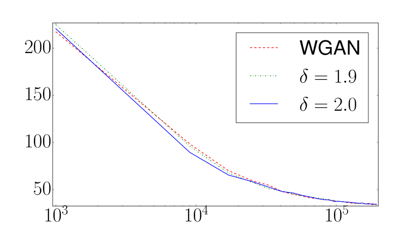
(a)

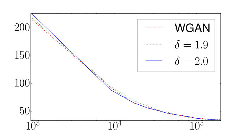
(b)

Figure 4: FID versus generator iteration on CIFAR10 for comparison of OTR WGAN and WGAN. Each subfigure presents a different initialization. These initializations are different from Figure 1. In the legend, $\delta$ is the OTR WGAN parameter.

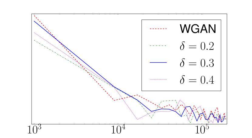
(a)

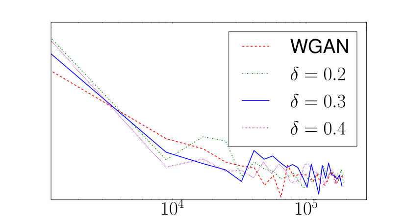
(b)

Figure 5: FID versus generator iteration on MNIST for comparison of OTR WGAN and WGAN. Each subfigure presents a different initialization. These initializations are different from Figure 2. In the legend, $\delta$ is the OTR WGAN parameter.

References

- [1] Soroosh Shafieezadeh Abadeh, Peyman Mohajerin Mohajerin Esfahani, and Daniel Kuhn. Distributionally robust logistic regression. In Advances in Neural Information Processing Systems, pages 1576–1584, 2015.
- [2] Charalambos D. Aliprantis and Kim C. Border. Infinite Dimensional Analysis. Springer, third edition, 2006.
- [3] Martin Arjovsky, Soumith Chintala, and Léon Bottou. Wasserstein generative adversarial networks. In International Conference on Machine Learning, pages 214–223, 2017.
- [4] Dimitri P Bertsekas. Convex optimization algorithms. Athena Scientific, 2015.
- [5] Jose Blanchet, Yang Kang, and Karthyek Murthy. Robust wasserstein profile inference and applications to machine learning. arXiv preprint arXiv:1610.05627, 2016.
- [6] Jose Blanchet and Karthyek Murthy. Quantifying distributional model risk via optimal transport. Mathematics of Operations Research, 2019.
- [7] Stéphane Boucheron, Gábor Lugosi, and Pascal Massart. Concentration Inequalities: A Nonasymptotic Theory of Independence. Oxford university press, 2013.
- [8] Marco Cuturi. Sinkhorn distances: Lightspeed computation of optimal transport. In Advances in Neural Information Processing Systems, pages 2292–2300, 2013.
- [9] RM Dudley. The speed of mean Glivenko-Cantelli convergence. The Annals of Mathematical Statistics, 40(1):40–50, 1969.
- [10] Peyman Mohajerin Esfahani and Daniel Kuhn. Data-driven distributionally robust optimization using the wasserstein metric: Performance guarantees and tractable reformulations. Mathematical Programming, 171(1-2):115–166, 2018.
- [11] R’emi Flamary and Nicolas Courty. Pot python optimal transport library, 2017.
- [12] Aden Forrow, Jan-Christian Hütter, Mor Nitzan, Philippe Rigollet, Geoffrey Schiebinger, and Jonathan Weed. Statistical optimal transport via factored couplings. In The 22nd International Conference on Artificial Intelligence and Statistics, pages 2454–2465, 2019.
- [13] Aude Genevay, Marco Cuturi, Gabriel Peyré, and Francis Bach. Stochastic optimization for large-scale optimal transport. In Advances in Neural Information Processing Systems, pages 3440–3448, 2016.
- [14] Ishaan Gulrajani, Faruk Ahmed, Martin Arjovsky, Vincent Dumoulin, and Aaron C Courville. Improved training of Wasserstein GANs. In Advances in Neural Information Processing Systems, pages 5767–5777, 2017.
- [15] Martin Heusel, Hubert Ramsauer, Thomas Unterthiner, Bernhard Nessler, and Sepp Hochreiter. GANs trained by a two time-scale update rule converge to a local Nash equilibrium. In Advances in Neural Information Processing Systems, pages 6626–6637, 2017.
- [16] Soheil Kolouri, Se Rim Park, Matthew Thorpe, Dejan Slepcev, and Gustavo K Rohde. Optimal mass transport: Signal processing and machine-learning applications. IEEE Signal Processing Magazine, 34(4):43–59, 2017.
- [17] Alex Krizhevsky and Geoffrey Hinton. Learning multiple layers of features from tiny images. Technical report, 2009.
- [18] Matt Kusner, Yu Sun, Nicholas Kolkin, and Kilian Weinberger. From word embeddings to document distances. In International Conference on Machine Learning, pages 957–966, 2015.
- [19] Yann LeCun. The mnist database of handwritten digits. http://yann. lecun. com/exdb/mnist/, 1998.
- [20] Ulrike von Luxburg and Olivier Bousquet. Distance-based classification with Lipschitz functions. Journal of Machine Learning Research, 5(Jun):669–695, 2004.
- [21] Paul Milgrom and Ilya Segal. Envelope theorems for arbitrary choice sets. Econometrica, 70(2):583–601, 2002.
- [22] Yu. Nesterov. Smooth minimization of non-smooth functions. Mathematical Programming, 103(1):127–152, 2005.
- [23] Tim Salimans, Ian Goodfellow, Wojciech Zaremba, Vicki Cheung, Alec Radford, and Xi Chen. Improved techniques for training GANs. In Advances in Neural Information Processing Systems, pages 2234–2242, 2016.
- [24] Maziar Sanjabi, Jimmy Ba, Meisam Razaviyayn, and Jason D Lee. On the convergence and robustness of training GANs with regularized optimal transport. In Advances in Neural Information Processing Systems, pages 7091–7101, 2018.
- [25] Maurice Sion. On general minimax theorems. Pacific Journal of Mathematics, 8(1):171–176, 1958.
- [26] Cédric Villani. Topics in Optimal Transportation. Number 58. American Mathematical Soc., 2003.
- [27] Jonathan Weed and Francis Bach. Sharp asymptotic and finite-sample rates of convergence of empirical measures in Wasserstein distance. arXiv preprint arXiv:1707.00087, 2017.