Ensemble Pruning via Margin Maximization

Abstract

Ensemble models refer to methods that combine a typically large number of classifiers into a compound prediction. The output of an ensemble method is the result of fitting a base-learning algorithm to a given data set, and obtaining diverse answers by reweighting the observations or by resampling them using a given probabilistic selection. A key challenge of using ensembles in large-scale multidimensional data lies in the complexity and the computational burden associated with them. The models created by ensembles are often difficult, if not impossible, to interpret and their implementation requires more computational power than single classifiers. Recent research effort in the field has concentrated in reducing ensemble size, while maintaining their predictive accuracy. We propose a method to prune an ensemble solution by optimizing its margin distribution, while increasing its diversity. The proposed algorithm results in an ensemble that uses only a fraction of the original classifiers, with improved or similar generalization performance. We analyze and test our method on both synthetic and real data sets. The simulations show that the proposed method compares favorably to the original ensemble solutions and to other existing ensemble pruning methodologies.

Keywords Quadratic Programming  $\cdot$ Ensemble Thinning  $\cdot$ Bagging  $\cdot$ Boosting  $\cdot$ Random Forests

1 Introduction

Ensemble methods combine a large number of fitted values (sometimes in the hundreds) into a bundled prediction. The output of an ensemble method is generally the combination of many fits of the same data set by either reweighting the observations or by using subsets of the original set obtained from bootstrapping, resampling or other probabilistic selections of the data. There is sufficient empirical evidence pointing to ensemble performance being generally superior to that of individual or single classifiers (Drucker et al., 1994; Breiman, 1996a, b; Quinlan, 1996; Schapire et al., 1998; Opitz and Maclin, 1999; Dietterich, 2000; Breiman, 2001; Maclin and Opitz, 2011). Boosting (Schapire, 1990) is one of the most well-known ensemble methods. The term boosting refers to a family of methods that combine weak classifiers (classification algorithms that perform at least slightly better than random) into a strong performing ensemble through weighted voting. AdaBoost (Freund and Schapire, 1997) is the leading implementation of boosting algorithms.

Among ensembles, Bagging (Breiman, 1996a), random forests (Breiman, 2001) and rotation forests (Rodriguez et al., 2006) are also strong performers in terms of their generalization ability. In addition to their ability to outperform individual classifiers, ensembles can also be very robust to overfitting, even when performing a large number of iterations (Quinlan, 1996; Schapire et al., 1998). To explain the successful performance of ensembles, Breiman (1999) suggested that boosting, bagging and random Forests (which he referred to as arcing classifiers) reduce the variance, in the bias-variance decomposition framework, however Schapire et al. (1998) refuted this claim by empirically providing evidence that AdaBoost mainly reduced the bias. More importantly, Schapire et al. (1998) showed that AdaBoost is especially effective at increasing the margins of the training data. Schapire et al. (1998) developed an upper bound on the generalization error of any ensemble, based on the margins of the training data, from which it was concluded that larger margins should lead to lower generalization error, everything else being equal (sometimes referred to as the “large margins theory"). The large margins theory has its roots in the margin separation framework in support vector machines (SVM) (Cortes and Vapnik, 1995).

The proliferation of large scale, high velocity data sets, often containing variables of different data types, creates challenges for most traditional statistical and machine learning classification techniques, but it does so, even more markedly, for ensembles. The term “big data" has been used to describe large, diverse and complex data sets generated from various sources. The volume, variety and velocity (known as the 3Vs) are the main characteristics to distinguish big data problems from others (Megahed and Jones-Farmer, 2013). A key drawback of fitting ensembles to large scale multidimensional data (big data) is their computational burden. The iterative nature of ensembles, as well as how complex the resulting solutions are, makes their implementation especially challenging. In addition, interpretations of ensemble predictions are not as straightforward as those of single classifiers and the implementation of the resulting models requires fitting the data through all of the iterations (sometimes in the hundreds) of the ensemble. A high number of iterations is oftentimes necessary to reap the benefits of the improved generalization performance provided by ensembles (Schapire et al., 1998; Dietterich, 2000). For this reason, recent research effort has concentrated in reducing ensemble sizes, also called ensemble pruning (thinning), while trying to maintain or improve their predictive accuracy (see, e.g., Partalas et al. 2006; Zhang et al. 2006; Martinez-Munoz et al. 2009; Chen et al. 2009; Tsoumakas et al. 2009; Zhang et al. 2009; Lu et al. 2010; Li et al. 2012; Dai 2013; Germain et al. 2015). There is also evidence that smaller ensembles perform as well as, or better than, their large counterparts (Zhou et al. 2002), but knowing how large they should be is still an open research question.

Ensemble pruning generally places additional computational costs on the training phase of the ensemble, due to the additional emphasis to identify a strong-performing subensemble, however a reduced ensemble translates into a more manageable and computationally less prohibitive model in the implementation phase (Chen et al., 2009). Of particular importance in ensemble pruning is obtaining an ensemble that takes into account not only the quality of the individual classifiers, but also their disagreement (Zhang and Zhang, 2009; Germain et al., 2015), that is, the effectiveness of ensembles depends also on the diversity of their componentwise classifiers, with the premise that more diverse classifiers perform better. Therefore, for high dimensional data sets, a more efficient algorithm could be constructed, if only the most diverse weak classifiers of the ensemble solution are taken into consideration in the final combination. In this article we propose an algorithm that produces a reduced, strong-performing subensemble by optimizing the diversity of the resulting classifiers and maximizing its lower margin distribution. The proposed method is a weight-based quadratic optimization that aims to tune the weights of a given ensemble, such that the pairwise correlations of the weak classifiers and the margin variance are minimized, while the lower percentiles of the margin distribution of the ensemble are maximized.

2 Preliminaries

We assume a set of $T$ weak classifiers (also called weak learners), $h_{t}(\textbf{x}),t=1,2,...,T$, is created from the space (finite) of classifiers $\mathscr{H}$, each of which takes a $p\times 1$ input vector x and produces a prediction $h_{t}(\textbf{x})\in\{-1,+1\}$ for a binary response variable Y. The combined classifier prediction of an ensemble with $T$ learners for a covariate vector x is given by:

$$f_{T}(\textbf{x})=\text{sign}\left(\sum_{t=1}^{T}\alpha_{t}h_{t}(\textbf{x})\right),$$ (1)

where $\text{sign}:\mathbb{R}\rightarrow\{-1,0,+1\}$, such that $\text{sign}(a)=-1$, when $a<0$, $\text{sign}(a)=+1$ if $a>0$ and $\text{sign}(a)=0$ if $a=0$ (when $\text{sign}(a)=0$, we randomly assign $\{-1,+1\}$ to $f_{T}$); $\alpha_{t}$ is the weight associated with the $t^{th}$ weak learner, where $0\leq\alpha_{t}\leq 1$ and $\sum_{t=1}^{T}\alpha_{t}=1$. The task of any ensemble or combined classifier $f$ is to create a set of weak learners and determine their associated weights $\{\alpha_{1},\alpha_{2},...,\alpha_{T}\}$ based on a training sample of data pairs $S=\{(\textbf{x}_{i},y_{i}),i=1,2,...,n\}$ generated independently and identically distributed (i.i.d) according to an unknown joint distribution $P_{XY}$, to produce a combined prediction with small generalization (also called risk of the classifier)

$$R[f]=E_{XY}g(y,f(\textbf{x})),$$ (2)

for a given loss function $g$. For the binary classification framework, the generalization error is defined as $P_{XY}\left[f(\textbf{x})\neq y\right]$, which is generally estimated by $\hat{P}_{S}\left[f_{T}(\textbf{x})\neq y\right]=\sum_{i=1}^{n}I(y_{i}\neq f_{T}(\textbf{x}_{i}))/n$, where $I(y_{i}\neq f_{T}(\textbf{x}_{i}))=1$ if $y_{i}\neq f_{T}(\textbf{x}_{i})$, and 0 otherwise. We denote $P_{XY}[a]$ as the probability of event $a$ under the unknown distribution $P_{XY}$, and $\hat{P}_{S}[a]$ as the empirical probability of $a$ under $S$. We use $P[a]$ and $\hat{P}[a]$, when it is clear which distribution we are referring to. The weights assigned to the weak learners $\{\alpha_{1},\alpha_{2},...,\alpha_{T}\}$ can be uniform, as in the case of random forests, or based the accuracy of the componentwise learners, as in the case of boosting. We will refer to the classifiers $h_{t}(\textbf{x})$ contained in an ensemble as weak learners, base learners or (individual) classifiers, and they are implemented by a base-learning algorithm B, that maps the input vector x to the binary response variable Y. Base-learning algorithms can be decision trees, neural networks, or any other kind of learning or statistical method. The construction of an ensemble is based on two main steps, i.e., generating the weak learners, and then combining them. The final combination is done with a linear function, but the final prediction can also be based on user-specified thresholds.

To explain the, generally superior, performance of ensembles, Schapire et al. (1998) showed that margins were an integral part in understanding how ensembles could generalize. The margin of the $i^{th}$ training observation is defined by:

$$m_{i}=m_{i}(\textbf{x}_{i},y_{i})=y_{i}\sum_{t=1}^{T}\alpha_{t}h_{t}(\textbf{x}_{i}).$$ (3)

The margin can be viewed as a measure of “confidence" of the prediction for the $i^{th}$ training observation and is equal to the difference in the weighted proportion of weak classifiers correctly predicting the $i^{th}$ observation and the weighted proportion of weak classifiers incorrectly predicting the $i^{th}$ observation, so that $-1\leq m_{i}\leq 1$. A margin value of $-1$ indicates that all of the weak learner predictions were incorrect, while a margin value of $+1$ indicates all of the weak learners correctly predicted the observation. Next, we will briefly define the most common ensembles to date: boosting (Schapire, 1990; Freund and Schapire, 1997), and random forests (Breiman, 2001). There are other ensemble methods that merit mention, but given the scope of this paper, we will only discuss these two.

2.1 Boosting Algorithms

Boosting refers to the idea of converting a weak learning algorithm into a strong learner, that is, taking a classifier that performs slightly better than random chance and improving (boosting) it into a classifier with arbitrarily high accuracy. Boosting originated from the PAC (probably approximately correct) learning theory (Valiant, 1984) and the question that Kearns and Valiant (1994) posed on whether a “weak” learning algorithm can be boosted into an arbitrarily accurate “strong" learner. AdaBoost, the most well-know boosting algorithm, has been shown to be a PAC (strong) learner. A strong PAC learner is formalized in the following definition:

Definition 1 (Kearns and Valiant, 1994). Let $\mathscr{F}$ be a class of concepts. For every distribution $P_{\textbf{X}Y}$, all concepts $f\in\mathscr{F}$ and all $\epsilon\in(0,1/2)$, $\delta\in(0,1/2)$, a strong PAC learner has the property that with probability at least $1-\delta$ the base learning algorithm B outputs a hypothesis $h$ with $P\left[h(\textbf{x})\neq f(\textbf{x})\right]\leq\epsilon$. B must run in polynomial time in $1/\epsilon$, and $1/\delta$ using only a polynomial (in $1/\epsilon$ and $1/\delta$) number of examples.

Boosting can be based on resampling or reweighting (Seiffert et al., 2008). The main goal of boosting methods is to give more voting power $\alpha_{t}$ to the weak learners or classifiers that perform the best. AdaBoost, for example, achieves this by iteratively using the same base-learning classifier, only modifying the weights of the observations $D_{i}^{t}$ at iteration $t$, therefore B must accept observation weights $D_{i}$ as inputs. AdaBoost adaptively places more emphasis on the training observations that were misclassified by the previous weak learner (iteration). The weight that each observation receives in round $t+1$ of the iterations is given by

$$D_{i}^{t+1}=\frac{D_{i}^{t}\exp⁡(-\alpha_{t}y_{i}h_{t}(\textbf{x}_{i}))}{Z_{t}},$$ (4)

where $Z_{t}=\sum_{i=1}^{n}D_{i}^{(t)}\exp\{-\alpha_{t}y_{i}h_{t}(\textbf{x}_{i})\}$ is a normalization constant. The weights of misclassified observations increase by a factor of $\exp⁡(\alpha_{t})$ at iteration $t$. The AdaBoost algorithm is described in Algorithm 1. The voting power of each base learner is given by $\alpha_{t}=\frac{1}{2}\ln\left(\frac{1-\epsilon_{t}}{\epsilon_{t}}\right)$, where more emphasis is given to those base learners with lower misclassification error $\epsilon_{t}$.

Algorithm 1 AdaBoost

1:$[Input]:S=\{(\textbf{x}_{i},y_{i}),i=1,...,n\}$ for $T$ iterations

2:$[Initialize]:D_{i}^{(1)}=\frac{1}{n}$

3:$[Loop]:$ do for $t=1,...,T$

4:(a) obtain $h_{t}$ on the sample set $\{S,D_{i}^{(t)}\}$

5:(b) set $\epsilon_{t}=\sum_{i=1}^{n}D_{i}^{(t)}I\left(y_{i}\neq h_{t}(\textbf{x}_{i})\right)$

6:(c) break if $\epsilon_{t}=0$ or $\epsilon_{t}\geq\frac{1}{2}$

7:(d) set $\alpha_{t}=\frac{1}{2}\ln\left(\frac{1-\epsilon_{t}}{\epsilon_{t}}\right)$

8:(e) update $D_{i}^{(t+1)}=\frac{D_{i}^{(t)}\exp\{-\alpha_{t}y_{i}h_{t}(\textbf{x}_{i})\}}{Z_{t}}$

9:$[Output]:f_{T}{\textbf{(x)}}=sign\left(\sum_{t=1}^{T}\alpha_{t}h_{t}(\textbf{x})\right)$

Other boosting variations proposed are based on modifying the observation weighting function (4) (see, e.g., LogitBoost (Friedman et al., 2000), MadaBoost (Domingo and Watanabe, 2000), Gradient Boosting (Friedman, 2001), Stochastic Gradient Boosting (Friedman, 2002), Local Boosting (Zhang and Zhang, 2008)), and although they address some of AdaBoost’s limitations, they have not been proven to be strong PAC learners as formulated in Definition 1. The applications of boosting methods can be extended to regression, and multiclass problems easily, however as mentioned before we will focus only on the binary classification problem.

2.2 Random Forests

Breiman (2001) defines a random forest (RF) as an algorithm “consisting of a collection of tree structured classifiers ${h_{t}(\textbf{x},\theta_{t}),t=1,...,T}$, where ${\theta_{t}}$ are independently and identically distributed random vectors." Each tree casts a unit vote for the most popular class at input x.

RFs inject randomness by growing each of the $T$ trees on a random subsample of the training data, and also by using a small random subset of the predictors at each decision node split. The RF method is similar to boosting in the fact that it combines classifiers that have been trained on a subset sample or a weighted subset, but they differ in the fact that boosting gives different weight to the base learners based on their accuracy, while random forests have uniform weights. There has been ample research on these ensemble methods and how they perform under different settings. For a more complete review on their performance, the reader is referred to Quinlan (1996); Maclin and Opitz (1997); Dietterich (2000), and Maclin and Opitz (2011).

2.3 Generalization Error Bound Based on Margins

Schapire et al. (1998) proved an upper bound on the generalization error of an ensemble that does not depend on the number of classifiers combined $T$. The generalization error bound is formalized in Theorem 1.

Theorem 1 (Schapire et al., 1998). Assuming that the base-classifier space $\mathscr{H}$ is finite, that is $\mathscr{\left|H\right|}<\infty$, and for any $\delta>0$ and $\theta>0$, then with probability at least $1-\delta$ over the training set $S$ with size $n$, every voting classifier $f$ satisfies the following bound:

$$P\left[f_{T}(\textbf{x})\neq y\right]\leq\hat{P}\left[m(\textbf{x},y)\leq\theta)\right]+O\left(\frac{1}{\sqrt{n}}\sqrt{\frac{\ln{n}\ln{\mathscr{\left|H\right|}}}{\theta^{2}}+\ln{\frac{1}{\delta}}}{}\right),$$ (5)

where $P\left[f_{T}(\textbf{x})\neq y\right]$ is the generalization error of the combined classifier, the term $\hat{P}\left[m(\textbf{x},y)\leq\theta\right]$ is the proportion of training set less than a value $\theta>0$. When the hypothesis space is infinite, the expression $\ln{n}\ln{\mathscr{\left|H\right|}}$ is replaced by $d\log_{2}(d/n)$, where $d$ is the VC-dimension of the space of all possible weak classifiers (a measure of complexity). Schapire et al. (1998) use this bound to provide an explanation for the superior performance of AdaBoost, which they show is highly effective at increasing the margins. Based on this bound, Schapire et al. (1998) concluded that larger margins should lead to lower generalization error, holding other factors constant, such as the cardinality of the hypothesis space $\mathscr{\left|H\right|}$, the sample size $n$, and $\delta$. This is sometimes referred to as the “large margins theory" (Grove and Schuurmans, 1998; Schapire et al., 1998; Mason et al., 2000; Shen and Li, 2010; Wang et al., 2011, 2012; Gao and Zhou, 2013; Cid, 2012; Martinez and Gray, 2014; Zhou, 2014). Given that maximizing the minimum margin has not yielded positive results in terms of generalization performance (see, e.g., Schapire et al. 1998, Grove and Schuurmans 1998), many authors have proposed optimizing other functions of the ensemble margin distribution instead. For instance, Reyzin and Schapire (2006) suggested maximizing the average or the median margin, while other researchers have proposed that minimizing the variance of the margins might be a key component in designing better performing ensembles (e.g., Shen and Li 2010).

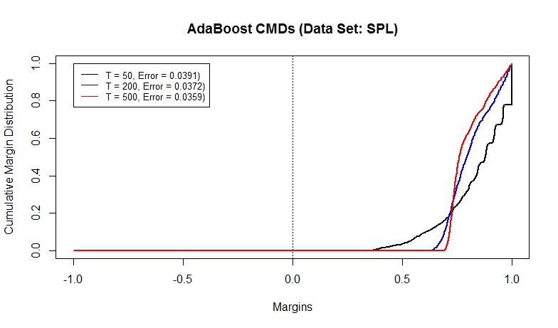
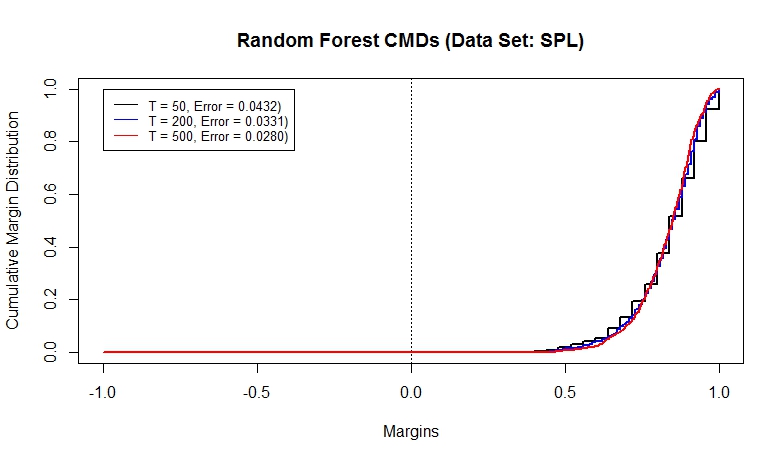
Figure 1 shows a typical behavior of the margins for a given ensemble. The cumulative margin distributions (CMDs) for ensembles of size $T=50,200,500$ are shown for AdaBoost and random forests for the SPL data set (see table 2 for data set description) using full-grown trees. As the ensemble size grows, the test set error (which is an estimate of the generalization performance) rate decreases for both type of ensembles using these settings. More importantly, we can see that the variation of the margins does appear to decrease as $T$ increases. An important observation of Figure 1 is that, as Schapire et al. (1998) noted, “boosting is especially aggressive at increasing the margins of the examples, so much so that it is willing to suffer significant reductions in the margins of those examples that already have large margins." This behavior is of particular significance, given that other researchers have shown that the lower margins play a pivotal role in ensemble performance (see, e.g., Guo and Boukir 2013). The improvement in the lower margins is evident in Figure 1 as the ensemble size grows, and it also corresponds closely to better generalization performance. This is more markedly visible in AdaBoost than the random forest solution.

(a)

(b)

Figure 1: Cumulative Margin Distributions (CMDs) for AdaBoost and Random Forests for $T=50,200,500$ for the SPL data set using full grown trees.

2.4 Relationship Between Ensemble Performance and Ensemble Diversity

A different, but no less important measure of effectiveness, is how diverse the individual classifiers within an ensemble are. Several researchers provide evidence on the importance of diversity within ensembles (Margineantu and Dietterich, 1997; Breiman, 2001; Kuncheva and Whitaker, 2003; Liu et al., 2004; Banfield et al., 2005; Brown et al., 2005; Blaser and Fryzlewicz, 2016). Li et al. (2012) proved an upper bound on the generalization error of any ensemble based on the diversity of its individual classifiers. The bound is given in Theorem 2.

Theorem 2 (Li et al., 2012). Assuming that for every $f$, there exists a set of $T$ classifiers $h_{t}(\textbf{x}),t=1,2,...,T$, satisfying $f_{t}(\textbf{x})=1/T\left(\sum_{t=1}^{T}h_{t}(\textbf{x})\right)$ and $div(f)\geq r$ for any i.i.d training set $S$ with size $n$, then for any $\epsilon$, and with probability at least $1-\delta$, for any $\theta>0$, every function $f$ satisfies the following bound:

$$P\left[f_{T}(\textbf{x})\neq y\right]\leq\hat{P}\left[m(\textbf{x},y)\leq\theta)\right]+\frac{C}{\sqrt{T}}\left(\frac{\ln{n}\ln{(T\sqrt{1/n+(1-1/n)(1-r)})}}{\theta^{2}}+\ln{\frac{1}{\delta}}\right),$$ (6)

where $C$ is a constant, $div(f)$ is any measure of diversity or disagreement among voters of a given ensemble $f$. The bound in (6) cannot be minimized directly, but it suggests that an increase in diversity should improve generalization performance, holding other factors constant, such as the complexity of the classifier and sample size. Note that this bound does depend on $T$.

Margineantu and Dietterich (1997) define diversity or disimilarities of ensembles based on either the probability distributions on which the weak learner are derived, or the agreement (disagreement) of the classifiers in their predictions. Several researchers have used the $\kappa$ and $\kappa$-error diagrams proposed by Margineantu and Dietterich (1997) to construct more diverse ensembles and/or evaluate their performance (see, e.g., Banfield et al. 2003; Kuncheva and Hadjitodorov 2004; Tsymbal et al. 2005; Rodriguez et al. 2006; Zhang and Zhang 2009). Germain et al. (2015) studied the relationship of ensemble diversity and the risk of majority voters, along with the first and second moments of the ensemble margins. They bounded the risk of a classifier with the expected disagreement between the individual learners. Germain et al. (2015) define $M(\textbf{x},y)$ as a random variable, that given an example $(\textbf{x},y)$ drawn according to $P_{XY}$, outputs the margin of the majority voter on that example, that is:

$$M(\textbf{x},y)=E_{XY}yf(\textbf{x}).$$ (7)

The generalization error, or risk of $f$, can then be defined in terms of the margins, as the probability that the majority voter is incorrect $R[f]=P\left[M(\textbf{x},y)\leq 0\right]$. An important characteristic of the random variable $M(\textbf{x},y)$ is its first moment defined as:

$$\mu_{M}=E_{XY}M(\textbf{x},y).$$ (8)

$\mu_{M}$ is estimated by $\bar{m}=\sum_{i=1}^{n}m_{i}(\textbf{x}_{i},y_{i})/n$, where $m_{i}(\textbf{x}_{i},y_{i})$ is the margin of the $i^{th}$ training observation. As previously stated, several authors have concluded that maximizing $\bar{m}$, or maximizing the whole margins distribution should improve the generalization performance, and that simply maximizing the minimum margin ($\min_{i}{m_{i}(\textbf{x}_{i},y_{i})}$) does not result in improved generalization performance (Schapire, 1999; Reyzin and Schapire, 2006; Grove and Schuurmans, 1998; Zhou, 2014). The second moment of the distribution of $M(\textbf{x},y)$ is also of particular importance. We define the second moment as:

$$\mu^{2}_{M}=E_{XY}M^{2}(\textbf{x},y).$$ (9)

Germain et al. (2015) provide an upper bound on the generalization error $R[f]$ of an ensemble that relates the diversity or expected disagreement between voters $(d_{S})$, which is a particular measure of $\text{div}(f)$ on distribution $S$, and the second moment of the margin distribution $\mu^{2}_{M}$. The bound is given in Theorem 3.

Theorem 3 (Germain et al., 2015). For any distribution $Q$ on a set of voters and any distribution $D$ ox $X$, if $\mu_{M}>0$, we have:

$$P\left[f_{T}(\textbf{x})\neq y\right]\leq 1-\frac{1-2R_{D}(G_{Q})}{1-2d^{D}_{Q}},$$ (10)

where $R_{D}(G_{Q})$ is the Gibbs risk and $1-2d^{D}_{Q}$ relates the risk of the classifier with the second moment of the margin distribution. The reader is referred to Germain et al. (2015) for a more complete explanation and the derivation of the bound, but the work in Germain et al. (2015) suggests that reducing the second moment $\mu^{2}_{M}$ of the margins of any given ensemble, should produce a more diverse and better performing classifier. Hypotheses presented by Reyzin and Schapire (2006), Shen and Li (2010) and Germain et al. (2015) all suggest that reducing the variation of the margins might also improve the generalization performance of an ensemble. Shen and Li (2010), for instance, proposed an algorithm named MD-Boost (Margin Distribution Boosting) that maximizes the average margin while reducing the variance of the margin distribution.

3 Existing Ensemble Pruning Methods

The idea on diversity-based pruning is to reduce the size of a given ensemble based on the similarity of the weak learners, working on the premise that a more diverse ensemble performs better, however there are various types of ensemble pruning methods, not necessarily based on diversity. Most of them fall into either selection-based methods, or weight-adjusting methods (Chen et al., 2009).

3.1 Selection-Based Methods

The main purpose of selection-based pruning methods is to either reject or select the given weak learner based on some criterion or criteria. The most common methodology used in selection-based pruning methods is to rank the weak learners within an ensemble according to some performance metric in a validation set and select a subset of the top $T_{r}$ out of the original $T$ weak learners. Margineantu and Dietterich (1997) proposed several measures of diversity and ways to prune ensembles accordingly. They proposed the use of the Kullback-Leibler divergence (KL distance) (Cover and Thomas, 1991) to prune ensembles, by maximizing the KL distance of the distribution upon which the classifiers were constructed. The KL distance between two probability distributions $p$ and $q$ is defined as:

$$D(q\left|\right|p)\leq q\ln\frac{q}{p}+(1-q)\ln\frac{1-q}{1-p},0\leq p,q\leq 1.$$ (11)

To measure the agreement (or disagreement) of ensemble predictions, Margineantu and Dietterich (1997) use the Kappa statistic ($\kappa$) (Kohen, 1960). Given two classifiers $h_{a}$ and $h_{b}$, Margineantu and Dietterich (1997) consider their agreement by constructing a contingency table with elements $C_{ij}$, where $i\in\{-1,+1\}$ and $j\in\{-1,+1\}$, corresponding to the number of observations for which $h_{a}(\textbf{x})=i$ and $h_{b}(\textbf{x})=j$, and

$$\theta_{1}=\frac{\sum_{i\in\{-1,+1\}}C_{ii}}{n}.$$ (12)

However, to account for class imbalances, the probability that the two classifiers agree is defined as:

$$\theta_{2}=\sum_{i\in\{-1,+1\}}\left(\frac{\sum_{i\in\{-1,+1\}}C_{ij}}{n}\frac{\sum_{i\in\{-1,+1\}}C_{ji}}{n}\right).$$ (13)

Finally, a measure of agreement $\kappa$ can be obtained by quantifying the likelihood to agree, compared to the expected agreement by chance:

$$\kappa=\frac{\theta_{1}-\theta_{2}}{1-\theta_{2}}.$$ (14)

The $\kappa$ measure in (23) has become a standard way to measure diversity in ensembles, and has been used extensively in selection-based pruning methods. Examples of other metrics used in selection-based methods include the margins of the ensemble and test set performance. For instance Martinez-Munoz and Suarez (2006) use classification performance on a test set based on orientation ordering to select the best subensemble, while Lu et al. (2010) and Li et al. (2012) proposed a heuristic to order the weak learners based on both their accuracy and their diversity. Prodromidis and Stolfo (2001) proposed reducing the size of ensembles by minimizing a cost complexity metric. Ordering the weak learners could also be based on their margins (e.g. Guo and Boukir 2013), or other measures that apply to specific types of analyses, such as time series (e.g., Ma et al. 2015). Other selection-based methods include formulating the selection of the pruned subsensemble as an integer optimization heuristic (e.g., Zhang et al. 2006). The list of selection-based pruning methods presented here is not exhaustive, the user is referred to Tsoumakas et al. (2009) for a more complete reference. One of the main limitations of most selection-based methods is that we must prespecify the size $T_{r}$ of the pruned subensemble. The selection-based approach is straightfoward, but does not guarantee the best possible subensemble and does not necessarily guarantee optimal performance.

3.2 Weight-Adjusting Methods

For weight-adjusting pruning methods, the main goal is not necessarily to prune the ensemble, but to adjust the weights of the weak learners, so that the generalization error is improved. In the process, some of the weights get zeroed out and consequently the ensemble is reduced (pruned). The main limitation of most weight-adjusting methods is that they do not have any theoretical guarantee to diminish the size of the ensemble, nor is there any explicit formulation to do so in their heuristics. For example Grove and Schuurmans (1998) used a linear programming technique to adjust the weights of the weak learners, so that the ensemble’s minimum margin is maximized. Grove and Schuurmans (1998) remark that the final ensemble was generally reduced significantly with their proposed algorithm. Demiriz et al. (2002) also used a weight-adjusting linear program to optimize a generalization error bound, which they show is also effective at pruning the ensemble. Chen et al. (2009) use expectation propagation to approximate the posterior estimation of the weight vectors. There are other weight-adjusting pruning methods in the literature that merit attention (e.g., Chen et al. 2006), and the reader is again referred to Tsoumakas et al. (2009) for a more exhaustive reference.

4 QMM (Quadratic Margin Maximization) Optimization Algorithm

In this section, we propose a weight-adjusting method based on quadratic programming to reduce the fraction of weak learners utilized in a particular ensemble. In designing our proposed algorithm, we take into account the generalization error bound in Theorem 1, which suggests that larger margins should lead to lower generalization error. Specifically, we focus on increasing the lower margin percentiles (Schapire et al., 1998). We also consider Theorem 2, which relates the performance of ensembles to the diversity of classifiers, with higher diverse classifiers expected to perform better, along with Theorem 3, which states that reducing the variance of the margins induces a more diverse and better performing combined classifier. The quadratic program formulation aims to tune the weights of the given ensemble, such that the pairwise correlations of the weak learners and the variance of the margins are minimized, while maximizing the lower percentiles of the margins.

4.1 Quadratic Programming (QP) Formulation

We assume that we are given an ensemble solution, i.e., a set of weak learners $h_{t}(\textbf{x}),t=1,2,...,T$, and a set of weights $\boldsymbol{\alpha}\in(0,1)^{T}$, where $\boldsymbol{\alpha}=\{\alpha_{1}\alpha_{2}\dots\alpha_{T}\}^{\top}$, where $0\leq\alpha_{t}\leq 1$ and $\sum_{t=1}^{T}\alpha_{t}=1$, associated with the weak classifiers. The weights $\alpha_{t}$ can be normalized without loss of generality. Note that for the training sample $S=\{(\textbf{x}_{i},y_{i}),i=1,2,...,n\}$ used to produce the ensemble solution, the values of the weak learner predictions $h_{it}$ and the weights $\alpha_{t}$ are fixed. We will let $h_{it}=\pm 1$ denote the prediction of the $t^{th}$ weak learner for the $i^{th}$ observation in the training data, $\textbf{y}=\{y_{1}y_{2}\dots y_{n}\}^{\top}$ and $\textbf{m}=\{m_{1}m_{2}\dots m_{n}\}^{\top}$ . We define the matrix

$$\textbf{H}_{n,T}=\begin{pmatrix}h_{11}&h_{12}&\cdots&h_{1T}\\ h_{21}&h_{22}&\cdots&h_{2T}\\ \vdots&\vdots&\ddots&\vdots\\ h_{n1}&h_{n2}&\cdots&h_{nT}\end{pmatrix},$$ (15)

where $\textbf{H}\in\{-1,1\}^{n\times T}$, as the predictions matrix for the $T$ weak classifiers within the ensemble. The error matrix $\textbf{E}=\textbf{H}\bullet\textbf{y}$ is defined as:

$$\textbf{E}_{n,T}=\begin{pmatrix}y_{1}h_{11}&y_{1}h_{12}&\cdots&y_{1}h_{1T}\\ y_{2}h_{21}&y_{2}h_{22}&\cdots&y_{2}h_{2T}\\ \vdots&\vdots&\ddots&\vdots\\ y_{n}h_{n1}&y_{n}h_{n2}&\cdots&y_{n}h_{nT}\end{pmatrix},$$ (16)

where $\textbf{E}\in\{-1,1\}^{n\times T}$, with element $E_{ij}=-1$ when the prediction of $j^{th}$ classifier for observation $i$ is incorrect, $+1$ otherwise. Note that $\textbf{E}\boldsymbol{\alpha}=\textbf{m}$. Let $\hat{\boldsymbol{\Sigma}}=\text{cov}(\textbf{E})$ be the sample covariance matrix of E, where $\hat{\boldsymbol{\Sigma}}$ is a symmetric positive definite matrix, with error variance of the each weak learner $h_{t}$ in the diagonals $\hat{\sigma}_{h_{t}}^{2}$, and the errors covariance for weak learners $i$ and $j$ in the off-diagonals $\hat{\sigma}_{h_{ij}}$.

$$\hat{\boldsymbol{\Sigma}}_{T,T}=\begin{pmatrix}\hat{\sigma}_{h_{1}}^{2}&\hat{\sigma}_{h_{12}}&\cdots&\hat{\sigma}_{h_{1T}}\\ \hat{\sigma}_{h_{21}}&\hat{\sigma}_{h_{2}}^{2}&\cdots&\hat{\sigma}_{h_{2T}}\\ \vdots&\vdots&\ddots&\vdots\\ \hat{\sigma}_{h_{T1}}&\hat{\sigma}_{h_{T2}}&\cdots&\hat{\sigma}_{h_{T}}^{2}\end{pmatrix}.$$ (17)

Let $m_{(1)}<m_{(2)}<\cdots<m_{(n)}$ denote the ensemble margins after arrangement in increasing order of magnitude, and the margin vector $\boldsymbol{\varphi}_{\upsilon}\in(-1,1)^{\lceil n\upsilon\rceil}=\{m_{(1)}m_{(2)}\cdots m_{(\lceil n\upsilon\rceil)}\}^{\top}$ for a given percentile $\upsilon$. We define the matrix $\Lambda_{\upsilon}\in(-1,1)^{\lceil n\upsilon\rceil\times T}$ as

$$\boldsymbol{\Lambda}^{\upsilon}_{\lceil n\upsilon\rceil,T}=\begin{pmatrix}y_{(1)}h_{(11)}&y_{(1)}h_{(12)}&\cdots&y_{(1)}h_{(1T)}\\ y_{(2)}h_{(21)}&y_{(2)}h_{(22)}&\cdots&y_{(2)}h_{(2T)}\\ \vdots&\vdots&\ddots&\vdots\\ y_{(\lceil n\upsilon\rceil)}h_{(\lceil n\upsilon\rceil 1)}&y_{(\lceil n\upsilon\rceil)}h_{(\lceil n\upsilon\rceil 2)}&\cdots&y_{(\lceil n\upsilon\rceil)}h_{(\lceil n\upsilon\rceil T)}\end{pmatrix},$$ (18)

such that

$$\boldsymbol{\Lambda}^{\upsilon}\begin{pmatrix}\alpha_{1}\\ \alpha_{2}\\ \vdots\\ \alpha_{T}\end{pmatrix}=\begin{pmatrix}m_{(1)}\\ m_{(2)}\\ \vdots\\ m_{(\lceil n\upsilon\rceil)}\end{pmatrix}.$$

The main goal is to minimize the error covariance matrix $\hat{\boldsymbol{\Sigma}}$, such that the lower $\upsilon$ margin percentiles are optimized. We call the quadratic program used to achieve this solution the QMM algorithm and it can be expressed in the following form:

minimize $$\textbf{w}^{\top}\hat{\Sigma}\textbf{w}$$ (19)

subject to $$\boldsymbol{\Lambda}^{\upsilon}\textbf{w}\geq\boldsymbol{\varphi}^{\upsilon}, \textbf{w}^{\top}\textbf{1}=1, \textbf{w}\geq\textbf{0},$$

where w are the new weights for the weak learners to be determined by solving the QP. The constraint $\Lambda^{\upsilon}\textbf{w}\geq\boldsymbol{\varphi}^{\upsilon}$ guarantees that the choice of w generates lower $\upsilon$ margin percentiles $\boldsymbol{\Lambda}^{\upsilon}\begin{pmatrix}w_{1}&w_{2}&\cdots&w_{T}\end{pmatrix}^{\top}$ at least as large, or larger than the lower $\upsilon$ margin percentiles generated by the ensemble $\boldsymbol{\Lambda}^{\upsilon}\begin{pmatrix}\alpha_{1}&\alpha_{2}&\cdots&\alpha_{T}\end{pmatrix}^{\top}$. Optimal solutions generally induce some of the w to equal zero, therefore reducing the final ensemble size, but the zeroing-out of the weights w is not guaranteed, as in most weight-adjusting pruning methods. The main hypothesis here is that reducing the error covariance, and minimizing the margin variance will cause the optimization algorithm to zero-out weights corresponding to the less diverse, worse performing weak learners.

One of the main issues that we can run into with QMM algorithm is the possibility of a less than full-rank H matrix because of column dependencies, which consequently would render the $\hat{\boldsymbol{\Sigma}}$ matrix also rank-deficient, and not positive semidefinite. Chen et al. (2009) use the least square pruning method ($lscov$) as a baseline before their proposed method to alleviate the rank deficient cases. We propose using a QR decomposition with pivoting to detect the column dependencies of H . If H has rank $r<\min{(n,T)}$, then there is an orthogonal matrix Q and a permutation matrix P such that

$$\textbf{Q}^{\top}\textbf{H}\textbf{P}=\begin{pmatrix}\textbf{I}_{r}&\textbf{0}_{r,T-r}\\ \textbf{0}_{n-r,r}&\textbf{0}_{n-r,T-r}&\\ \end{pmatrix},$$

The $r$ column pivot positions for H with indices $D_{H}=\{d_{1},d_{2},\cdots,d_{r}\}$ determine a basis for the number of columns needed to span the ensemble space of $T$ classifiers, while the $T-r$ non-pivot columns with indices $G=\{g_{1},g_{2},\cdots,g_{T-r}\}$ can be expressed as linear combinations of the $r$ pivot columns. Let $\boldsymbol{\alpha}^{\prime}=\{\alpha^{\prime}_{1}\alpha^{\prime}_{2}...\alpha^{\prime}_{r}\}^{\top}=\{\alpha_{d_{1}}\alpha_{d_{2}}...\alpha_{d_{r}}\}^{\top}$ denote the weights of the classifiers for the $r$ column pivot positions of H. Dropping the remaining $T-r$ columns of H, we obtain:

$$\textbf{H}^{\prime}_{n,r}=\begin{pmatrix}h^{\prime}_{11}&h^{\prime}_{12}&\cdots&h^{\prime}_{1r}\\ h^{\prime}_{21}&h^{\prime}_{22}&\cdots&h^{\prime}_{2r}\\ \vdots&\vdots&\ddots&\vdots\\ h^{\prime}_{n1}&h^{\prime}_{n2}&\cdots&h^{\prime}_{nr}\end{pmatrix}=\begin{pmatrix}h_{1d_{1}}&h_{1d_{2}}&\cdots&h_{1d_{r}}\\ h_{2d_{1}}&h_{2d_{2}}&\cdots&h_{2d_{r}}\\ \vdots&\vdots&\ddots&\vdots\\ h_{nd_{1}}&h_{nd_{2}}&\cdots&h_{nd_{r}}\end{pmatrix},$$ (20)

where $\textbf{H}^{\prime}$ is a full-rank matrix comprised $r\leq T$ classifiers, therefore also potentially pruning the ensemble. We also define the matrix $\textbf{H}^{*}=\textbf{H}/\textbf{H}^{\prime}$ as

$$\textbf{H}^{*}_{n,T-r}=\begin{pmatrix}h^{*}_{11}&h^{*}_{12}&\cdots&h^{*}_{1T-r}\\ h^{*}_{21}&h^{*}_{22}&\cdots&h^{*}_{2T-r}\\ \vdots&\vdots&\ddots&\vdots\\ h^{*}_{n1}&h^{*}_{n2}&\cdots&h^{*}_{nT-r}\end{pmatrix}=\begin{pmatrix}h_{1g_{1}}&h_{1g_{2}}&\cdots&h_{1g_{T-r}}\\ h_{2g_{1}}&h_{2g_{2}}&\cdots&h_{2g_{T-r}}\\ \vdots&\vdots&\ddots&\vdots\\ h_{ng_{1}}&h_{ng_{2}}&\cdots&h_{ng_{T-r}}\end{pmatrix}.$$ (21)

Let $\textbf{h}^{\prime}_{j},j=1,\cdots,r$ denote the $j^{th}$ column of $\textbf{H}^{\prime}$ with $\alpha^{\prime}_{r}$ associated weights, and $\textbf{h}^{*}_{k},k=1,\cdots,T-r$ the $k^{th}$ column of $\textbf{H}^{*}$ with $\alpha^{*}_{T-r}$ associated weights. If $r<\min{(n,T)}$ then $\textbf{h}^{\prime}_{j}=\sum^{G_{R}}_{i=1}(c_{i}\textbf{h}^{\prime}_{g})$, where $G_{R}$ is the number of columns from $\textbf{H}^{*}$ equal to $\textbf{h}^{\prime}_{j}$. Finally, the $j^{th}$ element of the weight vector for the classifier $\boldsymbol{\alpha}^{\prime}$ would be defined as:

$$\alpha^{\prime}_{j}=\sum^{G_{R}}_{i=1}(\alpha^{*}_{i}).$$ (22)

We would use $\textbf{H}^{\prime}$ and $\boldsymbol{\alpha}^{\prime}$ instead of H and $\boldsymbol{\alpha}$ in the QMM optimization formulation in (19) as a baseline, and the covariance matrix $\hat{\boldsymbol{\Sigma}}^{\prime}=\text{cov}(\textbf{H}^{\prime}\bullet\textbf{y})$ with the corresponding $\boldsymbol{\Lambda}^{\prime\upsilon}$ and $\boldsymbol{\varphi}^{\prime\upsilon}$. Therefore even if H is less than full-rank, the optimization would still be based on a full-rank $\hat{\boldsymbol{\Sigma}}^{\prime}$ matrix. It is also possible that $\hat{\boldsymbol{\Sigma}}$ is a full rank matrix but not positive semidefinite, especially in the case where $n<T$. In that case, the QMM algorithm will fail to find an optimal solution, and the resulting ensemble solution will be the original $f_{T}(\textbf{x})=\text{sign}(\textbf{E}\boldsymbol{\alpha})$ or most likely $f_{T}(\textbf{x})=\text{sign}(\textbf{E}^{\prime}\boldsymbol{\alpha}^{\prime})$. All the steps of the QMM algorithm are summarized in Algorithm 2.

Algorithm 2 QMM Algorithm

1:$[Input]:S$, $\textbf{H}=\{h_{it}\},t=1,...,T$, $\boldsymbol{\alpha}=\{\alpha_{1}\alpha_{2}...\alpha_{T}\}^{\top}$, m, and $\upsilon$ from Algorithm 1

2:$[Compute]:\textbf{H}^{\prime}$, $\boldsymbol{\alpha}^{\prime}$, $\hat{\boldsymbol{\Sigma}}$, and $\boldsymbol{\Lambda}^{\upsilon}$. Let $\textbf{H}\doteq\textbf{H}^{\prime}$, $\boldsymbol{\alpha}\doteq\boldsymbol{\alpha}^{\prime}$, $\boldsymbol{\Lambda}^{\upsilon}\doteq\boldsymbol{\Lambda}^{\prime\upsilon}$, and $\boldsymbol{\varphi}^{\upsilon}\doteq\boldsymbol{\varphi}^{\prime\upsilon}$

3:$[Optimize]:$ minimize $\textbf{w}^{\top}\hat{\boldsymbol{\Sigma}}\textbf{w}$ subject to $\boldsymbol{\Lambda}^{\upsilon}\textbf{w}\geq\boldsymbol{\varphi}^{\upsilon},\textbf{w}^{\top}\textbf{1}=1,\textbf{w}\geq 0$

4:$[Return]:\textbf{w}$

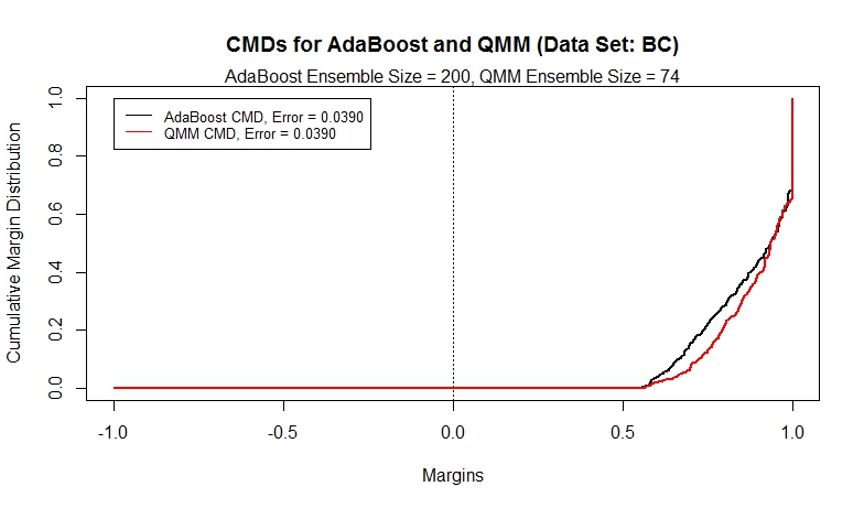
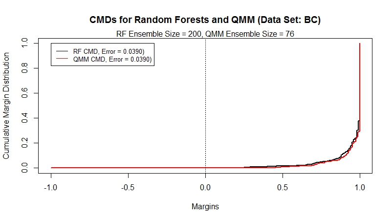
We illustrate the performance of the QMM algorithm in Figure 4 by plotting the cumulative margin distributions (CMDs) for the original AdaBoost and random forest solutions and the proposed QMM method on the Breast Cancer (BC) data set (see table 1 for data set description). The QMM ensemble uses only 74 trees (4-node, depth = 2) out of the 200 used by the AdaBoost solution, and 76 trees out of the random forest solution of 200 trees with equal error rates.

(a)

(b)

Figure 2: By round comparison of AdaBoost and MMI algorithm for the Splice data set using decision trees with 4 terminal nodes

4.2 Choice of $\upsilon$

The parameter $\upsilon$ determines the fraction of margins that will be maximized, that is, the QMM solution will constraint these margins to be at least as large as those of the original ensemble solution. Selecting a high value of $\upsilon$ will require a higher fraction of margins to be improved or maintained and since AdaBoost and random forests are highly effective at increasing the training margins (Schapire et al., 1998), the optimization will likely fail to find a feasible set. For $\upsilon=1$ we would likely obtain the original solution $\textbf{w}=\boldsymbol{\alpha}$ or an even an infeasible solution in the optimization algorithm, in which case we also assign $\textbf{w}=\boldsymbol{\alpha}$. On the other hand, setting $\upsilon$ close to 0 would most likely result in a smaller but underperforming ensemble. The selection of $\upsilon$ can be based on cross-validation, but this will result in higher computational costs. Making use of the structure of the margins distribution for the particular ensemble might also give some useful insights. For instance, Wang et al. (2011) developed an upper bound based on a single margin instance called the equilibrium margin (EMargin) as an explanation of the performance of ensemble methods. To explain the EMargin, we use the Bernoulli Kullback-Leiler function $D(q\left|\right|p)$ as defined in (6). $D(q\left|\right|p)$ is a monotone increasing function for a fixed $q$ and $q\leq p<1$. We can also see that $D(q\left|\right|p)=0$ when $p=q$ and $D(q\left|\right|p)\rightarrow\infty$ as $p\rightarrow 1$. The bound that relates the EMargin to the performance of an ensemble classifier is presented in Theorem 4.

Theorem 4 (Wang et al., 2011). Assuming that the base-classifier space $\mathscr{\left|H\right|}$ is finite, and for any $\delta>0$ and $\theta>0$, then with probability at least $1-\delta$ over the training set $S$ with size $n$, every voting classifier $f$ satisfies the following bound:

$$P\left[f_{T}(\textbf{x})\neq y\right]\leq\frac{\ln{\mathscr{\left|H\right|}}}{n}+\inf_{q\in\left(0,\frac{1}{n},\frac{2}{n},...,1\right)}D^{-1}\left(q;u\left[\hat{\theta}(q)\right]\right),$$ (23)

where $u\left[\hat{\theta}(q)\right]=\frac{1}{n}\left(\frac{8\ln\mathscr{\left|H\right|}}{\hat{\theta}^{2}(q)}\ln\left(\frac{2n^{2}}{\ln\mathscr{\left|H\right|}}\right)+\ln{\mathscr{\left|H\right|}}+\ln\frac{1}{\delta}\right)$ and

$$\hat{\theta}(q)=\sup_{\theta\in\left(\sqrt{\frac{8}{\mathscr{\left|H\right|}}},1\right]}\hat{P}\left[m(\textbf{x},y)\leq\theta)\right]\leq q.$$ (24)

The optimal value of $q$ in (23) defined as $q^{*}$ and evaluated at $\hat{\theta}(q^{*})$ is called the EMargin, while $q^{*}$ is called the EMargin error. Wang et al. (2011) suggest that an ensemble with higher EMargin $\hat{\theta}(q^{*})$ and lower EMargin error $q^{*}$ should perform better, holding everything else constant. With these results in mind, the value of $\upsilon$ can be set to $\hat{P}\left[m(\textbf{x},y)\leq\hat{\theta}(q^{*})\right]=\upsilon$.

The main drawback of using the EMargin to select the value of $\upsilon$ is the extra computational cost, as well as the difficulties in obtaining the size of the base-classifier space $\mathscr{\left|H\right|}$. Wang et al. (2011) suggested using a preespecified number of thresholds uniformly distributed on $\left[0,1\right]$ on each feature with a fixed classifier complexity, such as decision stumps, so that $\mathscr{\left|H\right|}$ can be computed accurately.

(a)

(b)

Figure 3: Performance of the QMM algorithm under different values of $\upsilon$ for AdaBoost and Random Forests using full-grown trees. The shaded grey represents the fraction of weak learners used given the ensemble size, while the red and black curves represent the test set error rates of the QMM algorithm and AdaBoost respectively.

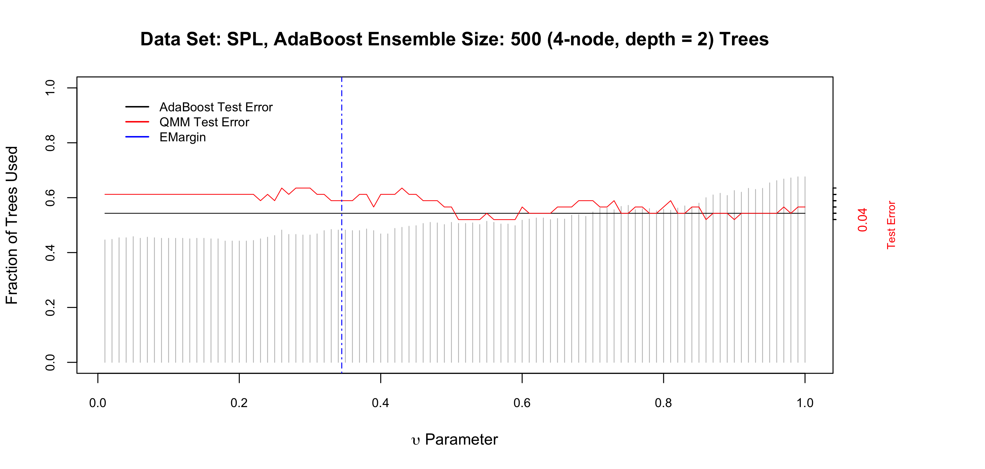
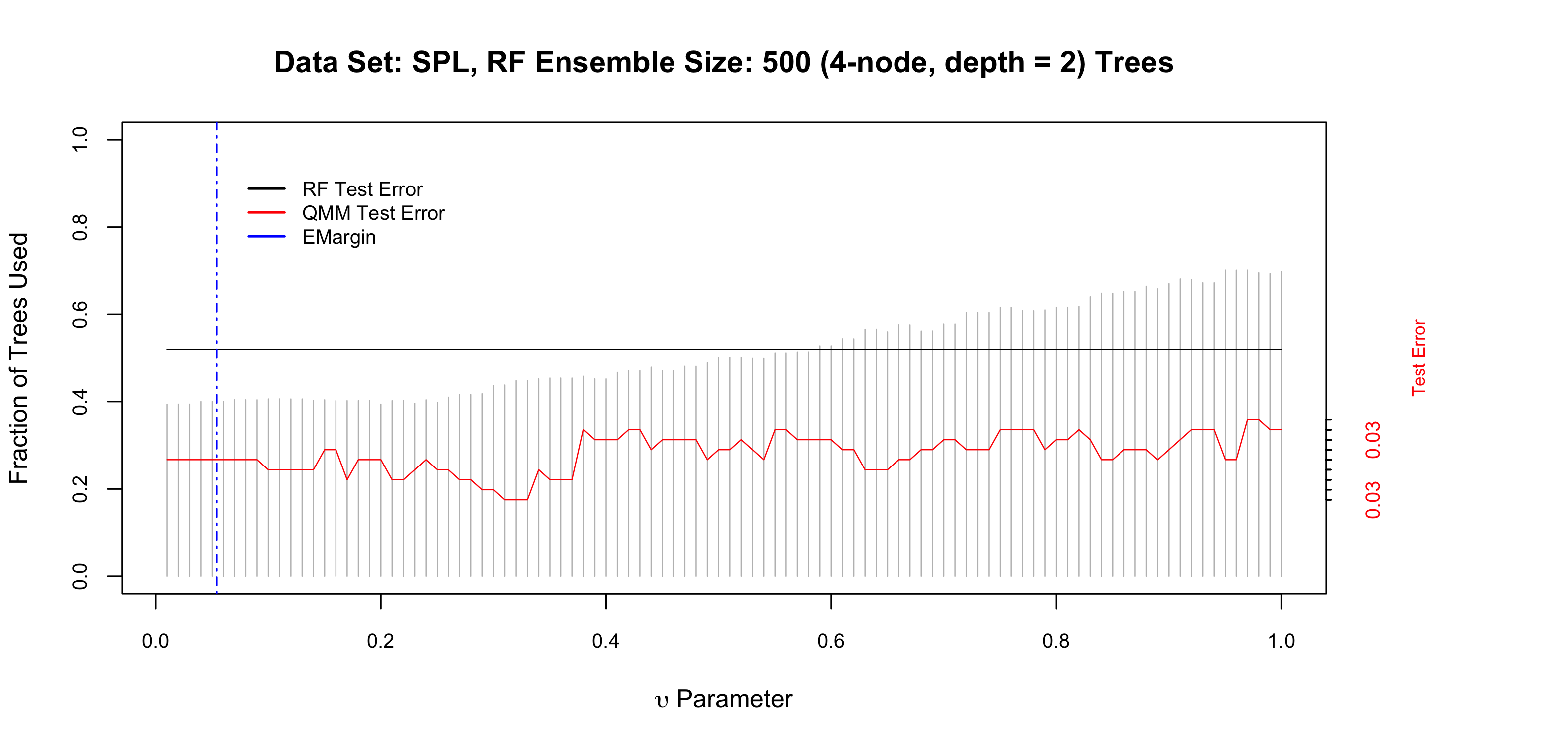
Figure 3 illustrates the performance of the QMM algorithm for the SPL data set under different values of $\upsilon$ for both AdaBoost and random forests. We fix the complexity and obtain the size of hypothesis space by using 4-node (depth = 2) decision trees. We further normalize each feature of the SPL data set to $\left[0,1\right]$ and consider only 100 thresholds uniformly distributed on $\left[0,1\right]$ on each feature, so that $\mathscr{\left|H\right|}=\left(2\times 100\times p\right)^{3}$, where $p=60$. We then obtain the fraction of trees used, the test set error rate for values of $\upsilon=(0,1]$ with increments of $0.01$. This specific example shows that lower values of $\upsilon$ correspond to the highest ensemble pruning rate for both AdaBoost and random forests, however it translates to worse performance for the AdaBoost algorithm. For higher values of $\upsilon$, it becomes increasingly more difficult for the algorithm to prune the ensemble and consequently the QMM algorithm yields a higher fraction of trees selected. It is clear that the optimal value of $\upsilon$ depends on the ensemble type, as well as the data set used. The vertical dotted blue line in Figure 3 corresponds to the EMargin. The example in Figure 3 is a typical performance of the QMM algorithm and shows that the performance of the QMM algorithm is better for higher values of $\upsilon$ with an AdaBoost solution, while values of $\upsilon$ ranging from 0.01 to 0.40 result in improved performance in random forests. Using the EMargin to set the parameter $\upsilon$ generally results in a higher pruning rate with acceptable performance results, however to reduce computational costs in our simulations, we have set $\upsilon=0.5$ for AdaBoost, and $\upsilon=0.25$ for random forests knowing that this value could be further optimized by different means that not are limited to the use of the EMargin, but can also be derived by cross validation, especially if computational costs for the specific problem are not an issue. For further simulations, we do not restrict the decision trees to a preespecified number of thresholds.

Table 1: Description of Data Sets (Low Dimensional)

Data Set	Description	Source	Train	Test	Features
AU	Australian Credit Approval	Lichman (2013)	482	208	14
BAN	Banana Data Set	Rätsch (2014)	3710	1590	2
BC	Breast Cancer Wisconsin	Lichman (2013)	478	205	10
DIA	Diabetes Patient Records	Lichman (2013)	537	231	8
FC	Fourclass Non-Separable	Ho and Kleinberg (1996)	603	259	2

5 Experiments and Simulations

The application of the QMM algorithm is illustrated on several synthetic and real data sets to gauge its applicability. We compare the performance of QMM algorithm to the original ensemble using the test set error rate and the percentage of the weak learners used at a given ensemble size. Tables 1, 2 and 3 show descriptions and properties of the data sets utilized in the simulations. Data sets that do not contain a validation data set were split on a 70/30 sampling scheme. The data sets range in size and dimensionality. We have arbitrarily broken down the data sets into three main types: low dimensional data sets (Table 1), mid dimensional data sets (Table 2), and high dimensional data sets (Table 3). The ensembles used for the this analysis are AdaBoost and random forests. If the QMM algorithm does not result in a feasible solution we have provided alternative decreasing values of $\upsilon$. For AdaBoost, we have set the following options $\upsilon\in\{0.50,0.25,0.05,0.01\}$, and for random forests $\upsilon\in\{0.25,0.15,0.05,0.01\}$.

5.1 QMM Performance

Table 2: Description of Data Sets (Mid Dimensional)

Data Set	Description	Source	Train	Test	Features
IJC	IJCNN 2001 Competition	Prokhorov (2001)	49990	91701	22
ION	Ionosphere Data Set	Lichman (2013)	245	106	34
MR	Mushrooms Data Set	Lichman (2013)	5686	2438	112
SON	Sonar Data Set	Lichman (2013)	145	63	60
SPL	DNA Splice Junctions	Lichman (2013)	1000	2175	60

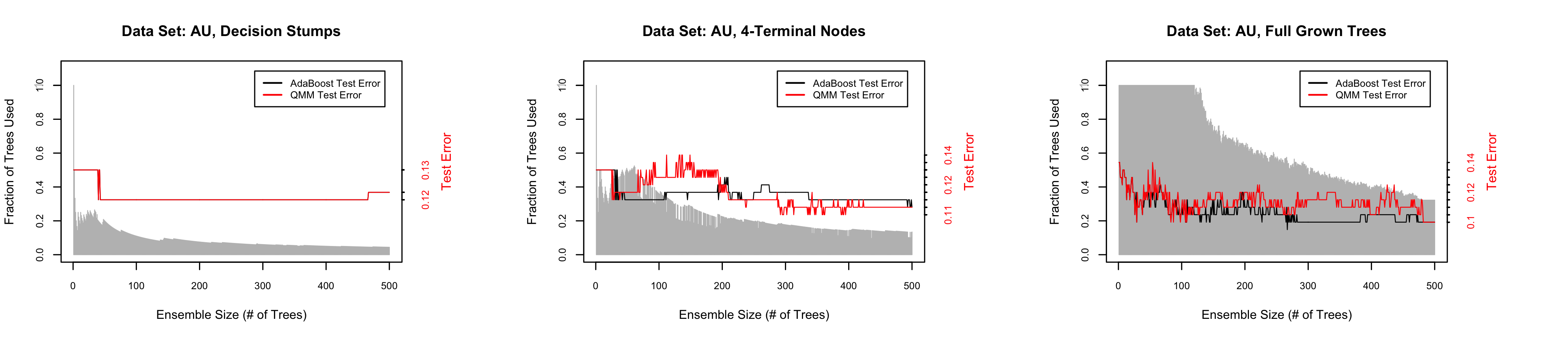
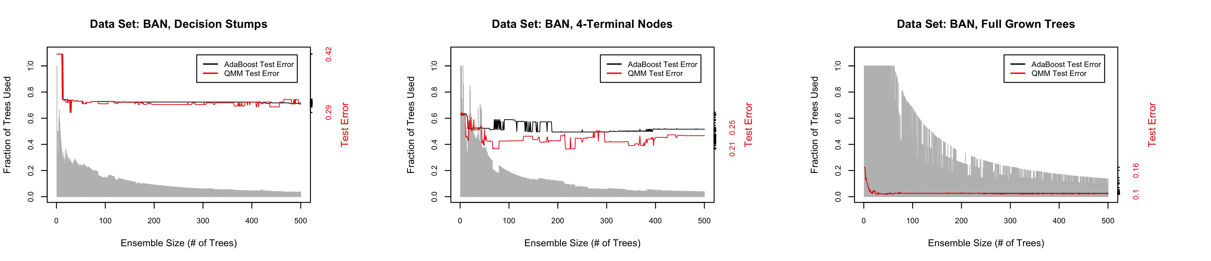
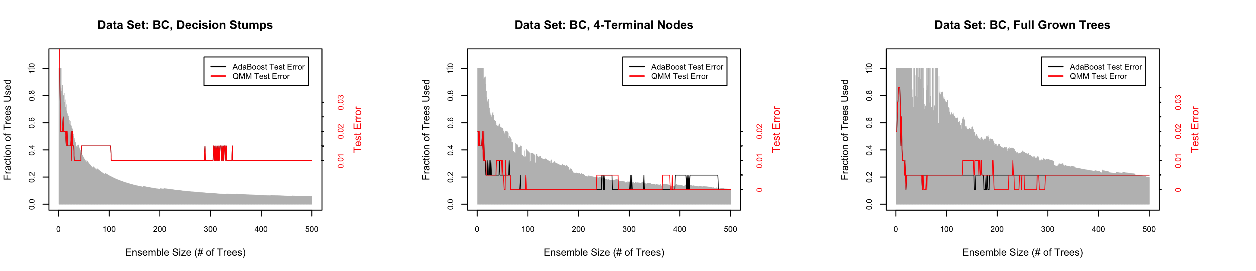
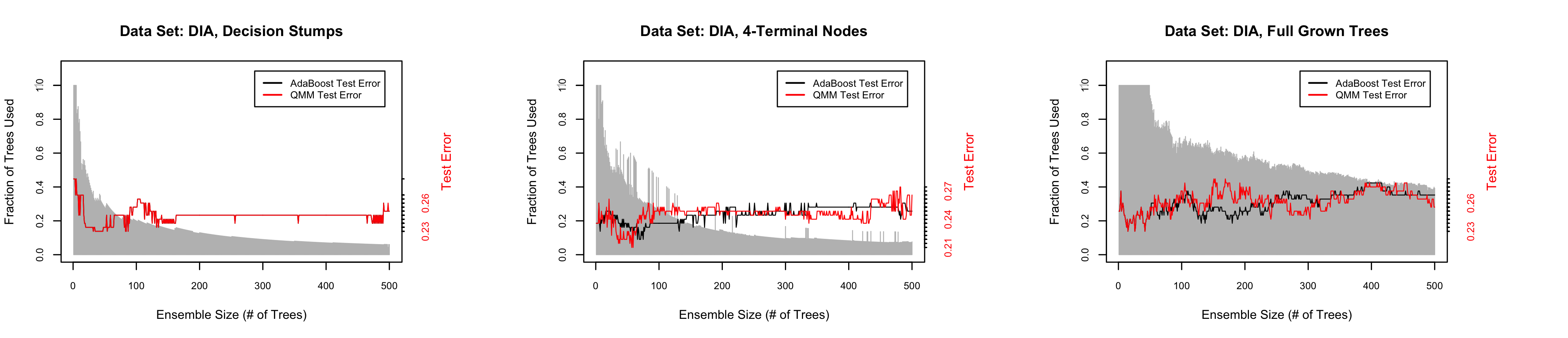
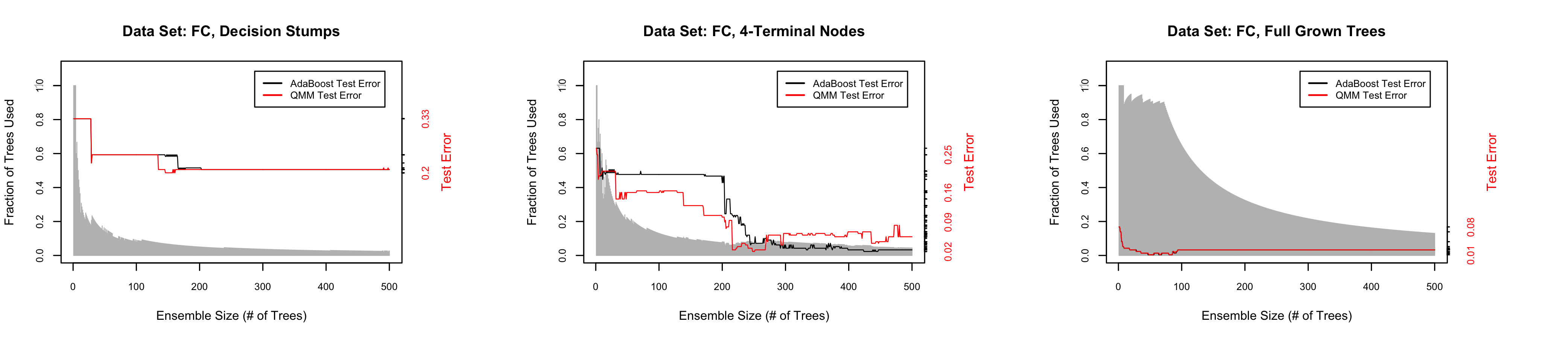
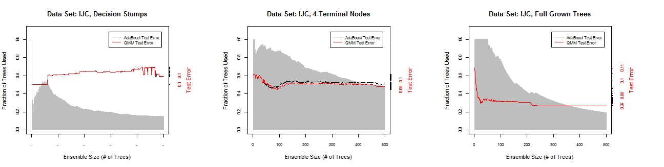
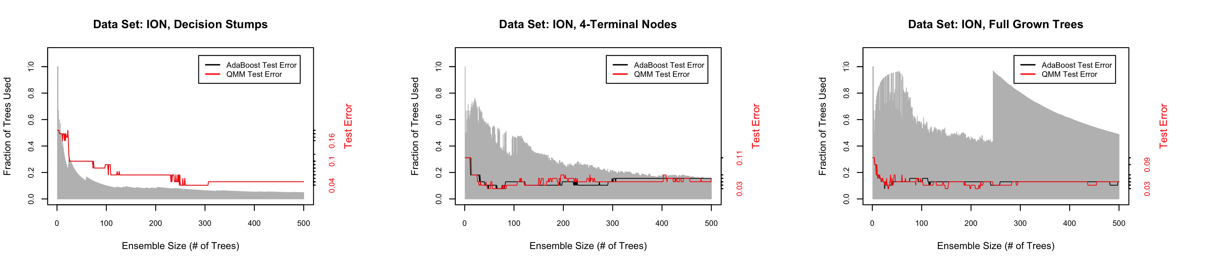
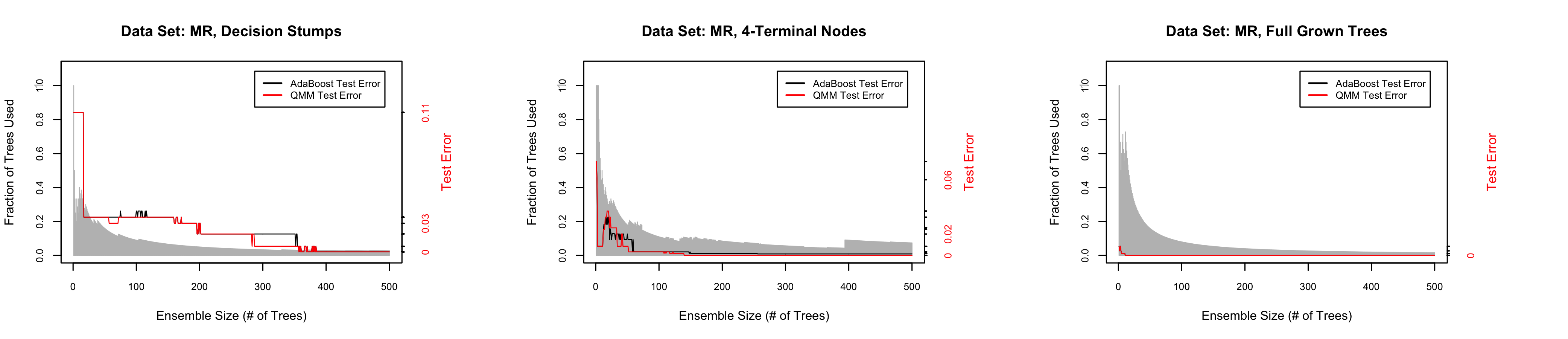
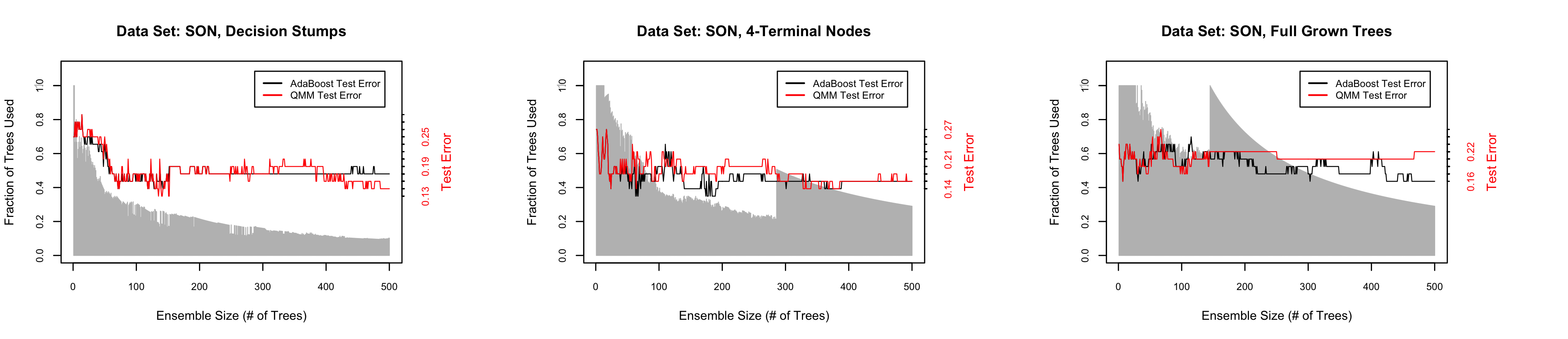
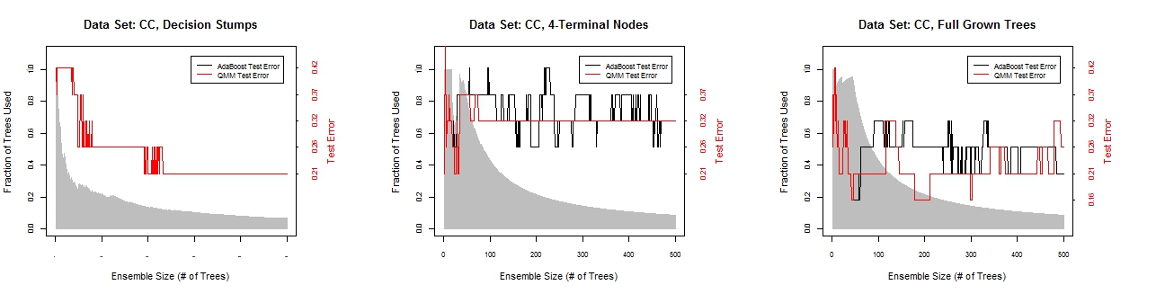
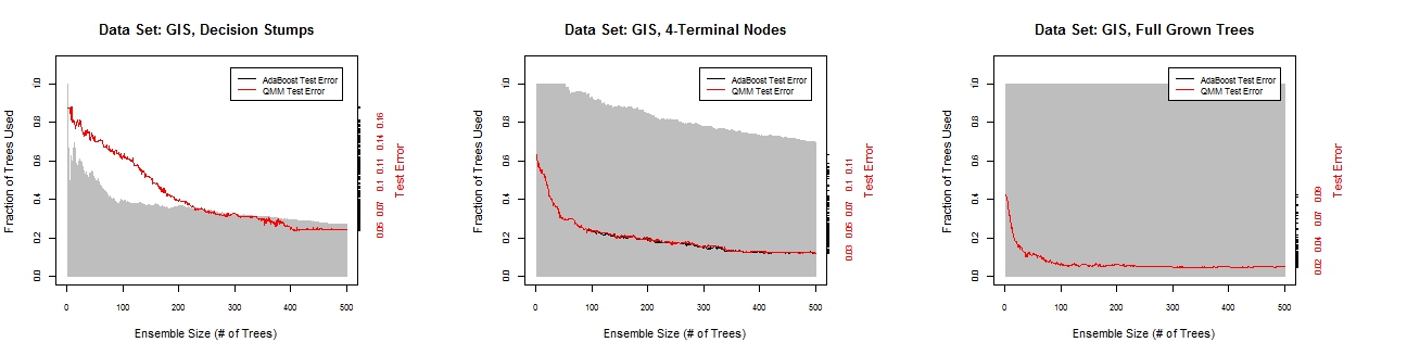
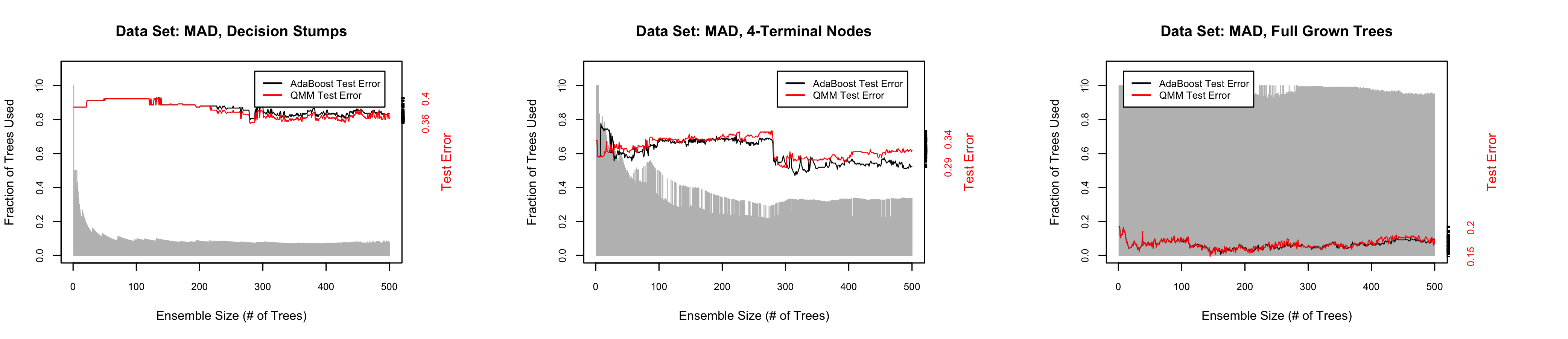
Figure 5 illustrates the test error curves and percentage of trees utilized for the QMM algorithm versus the original AdaBoost on low dimensional data sets. The ensemble is grown to a size $T=500$. The shaded grey area represents the fraction of weak learners used for the given ensemble size, while the red and black curves represent the test set error rates of the QMM algorithm and AdaBoost respectively. We have used different topologies of CART classification trees (Breiman et al., 1984) that include decision stumps, 4-node (depth = 2) trees and full-grown trees as our base-learning classifiers. We can see in Figure 5 that the test set error rates of the QMM algorithm are comparable and sometimes outperform those of AdaBoost. The QMM algorithm only uses a fraction of the classifiers given by the AdaBoost solutions. As $T$ increases, the number of decision trees selected by the QMM algorithm decreases. This happens more markedly for ensembles of decision stumps. For instance, for low dimensional data sets on average only 22 trees out of an ensemble of size $T=500$ are assigned positive weights by the QMM algorithm, a 95.6% reduction. As the complexity of the classifier increases, a higher diversity is expected within the ensemble members. For 4-node trees, the ensemble is on average pruned to only 40.2 out of 500 trees, which suggests that the fraction of trees used by the QMM algorithm is generally higher as the tree depth increases. This is likely due to the fact that a less complex tree topology will induce more similar resulting trees. For full-grown trees the QMM algorithm prunes the AdaBoost ensemble to an average of 120 trees out of 500. The performance of the QMM algorithm in mid dimensional data sets does not differ significantly from low dimensional data sets as illustrated in Figure 6 . On average 37.8, 134 and 149.6 trees out 500 were selected for decision stumps, 4-node trees and full-grown trees respectively, which might also suggest lower pruning rates as the dimensionality of the data set increases. Results also indicate a similar performance of the resulting ensemble of the QMM algorithm compared to AdaBoost in terms of generalization ability. An interesting phenomenon happens for ION and SON data sets, showing a sudden increase in the percentage of trees used right after $T>n$, and this is likely due to the fact that $\hat{\boldsymbol{\Sigma}}^{\prime}$ is not positive semidefinite for data sets with $n<T$, nevertheless the QR decomposition of the H matrix reduces the size of the ensemble even if the QP formulation fails to find any feasible solution to prune the ensemble further. Figure 7 shows the performance of the proposed method for high dimensional data sets, which suggests a similar story to the low and mid dimensional data sets simulations. On average 67.3, 164.7 and 327 trees out 500 were used for decision stumps, 4-node trees and full-grown trees respectively. The trend further suggests that as the dimensionality of the data set increases, a higher number of trees is needed to achieve feasibility in the constraints of the QMM algorithm. An interesting note for the simulations on AdaBoost ensembles is that on occasions the percentage of trees varies wildly as $T$ increases for some data sets and this is due to the algorithm going back and forth to different values of $\upsilon$.

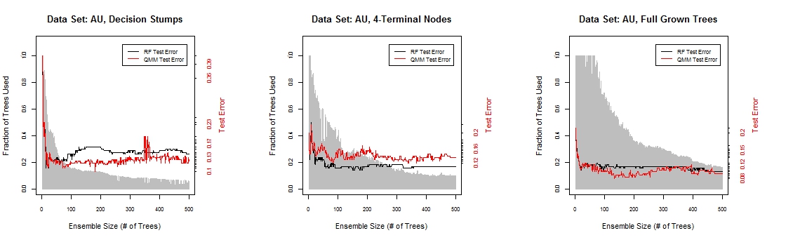
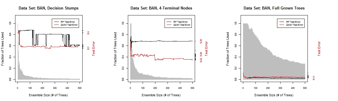
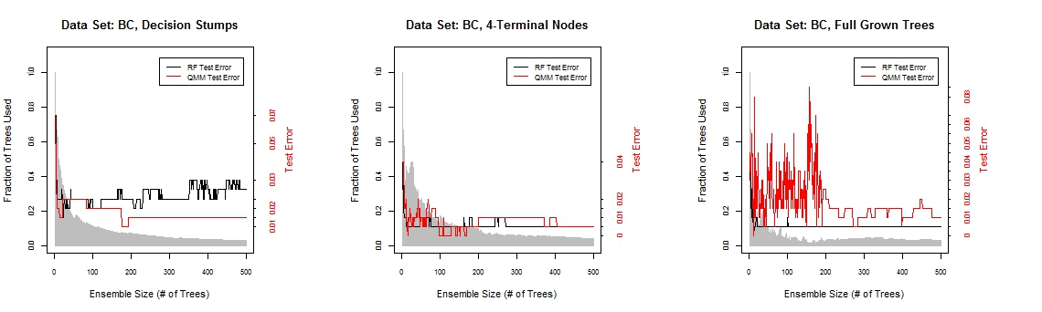
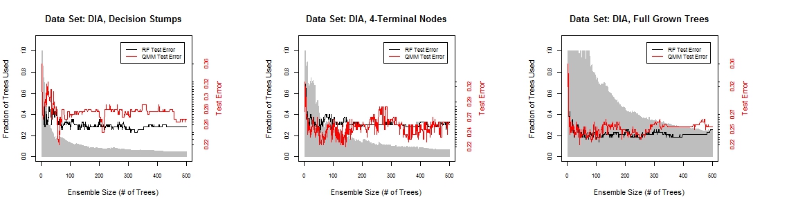
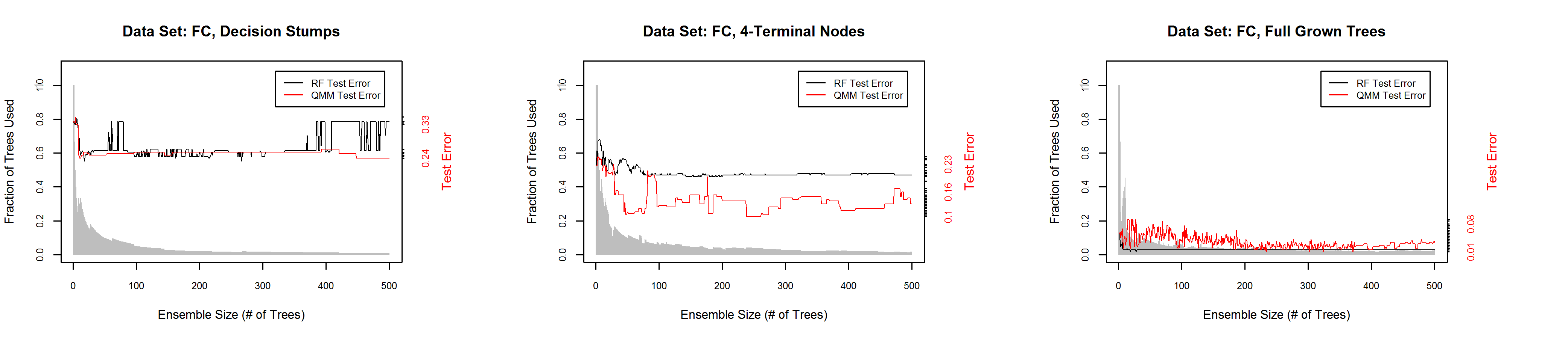
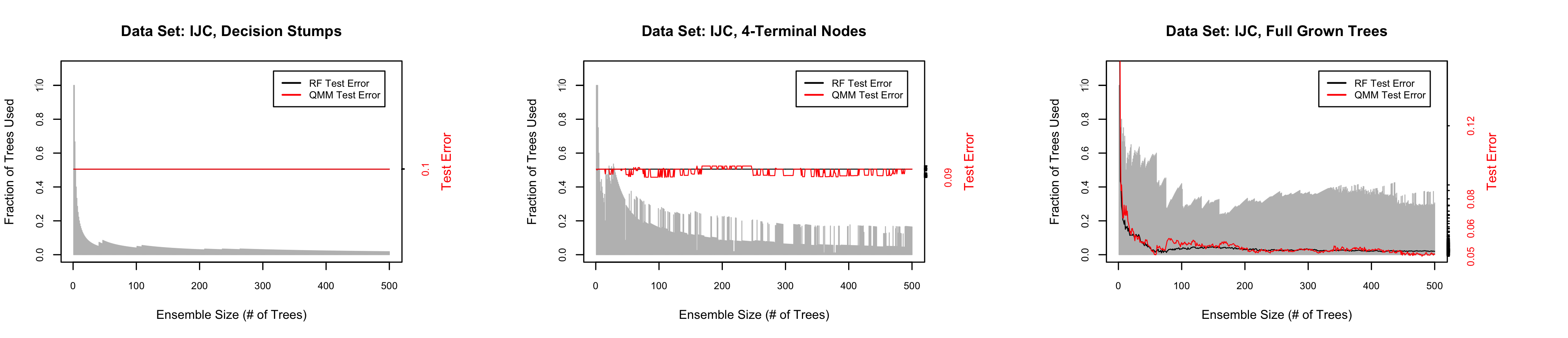
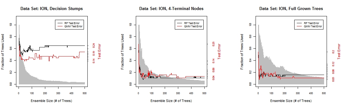
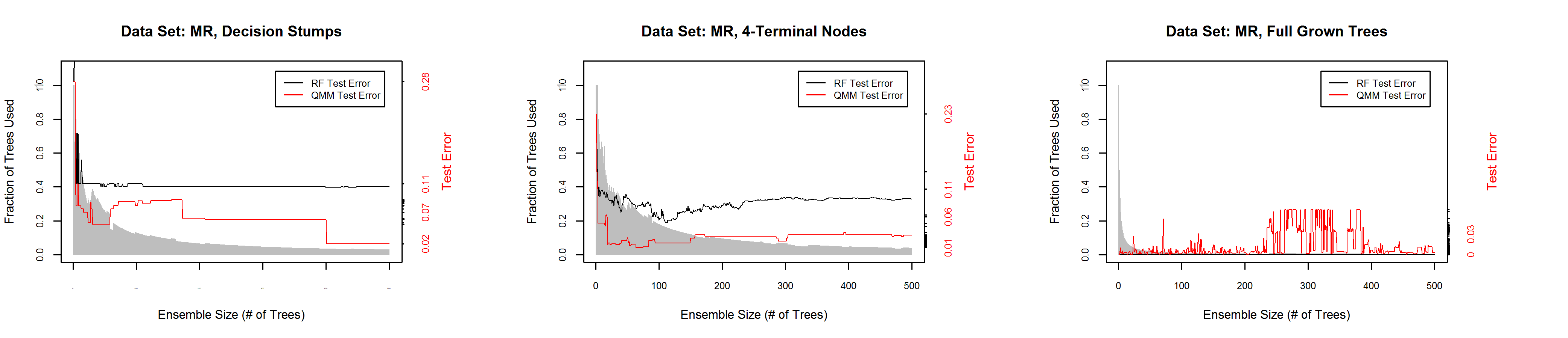
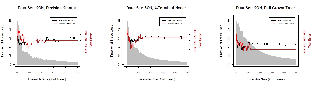
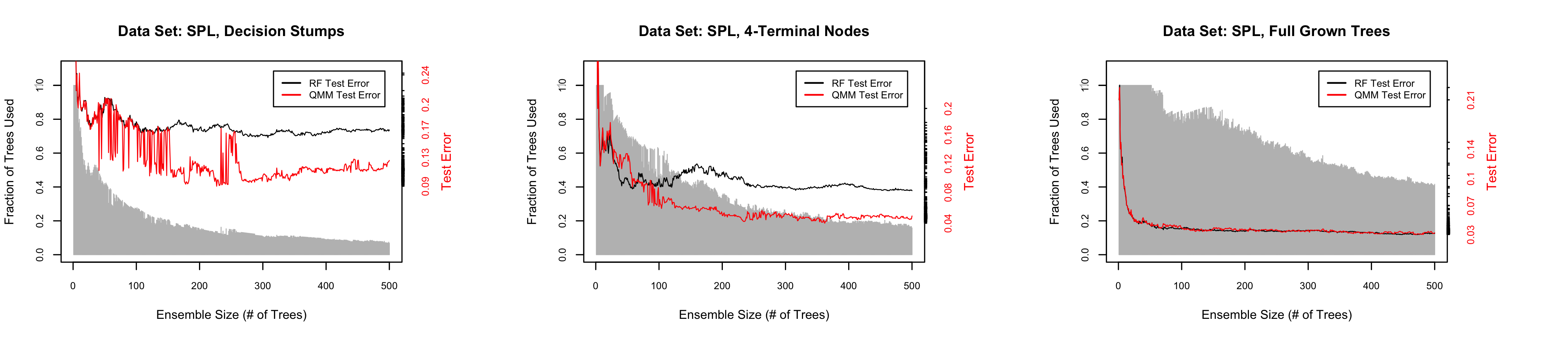
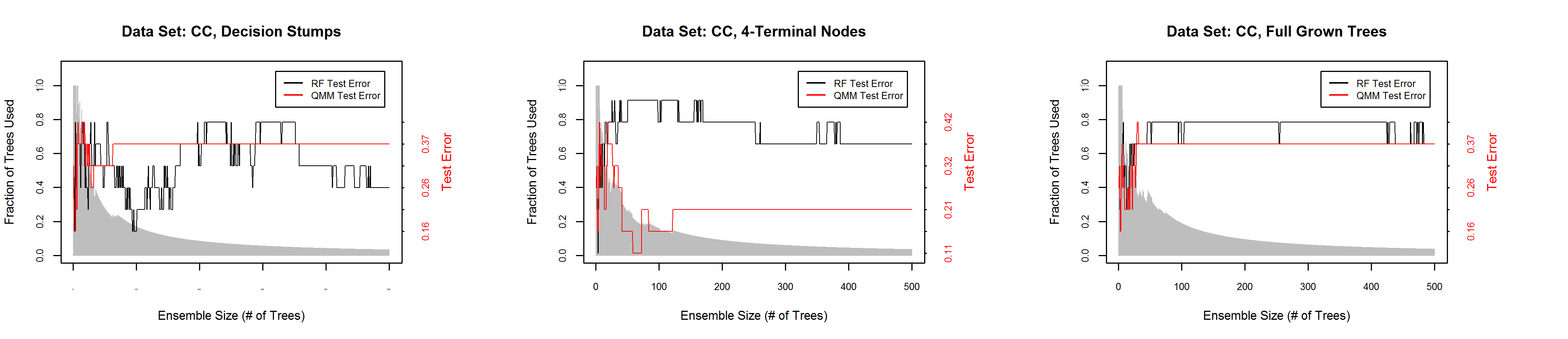
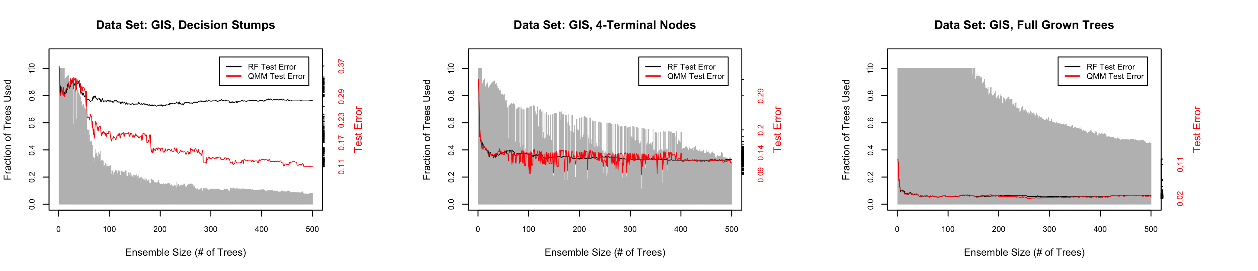
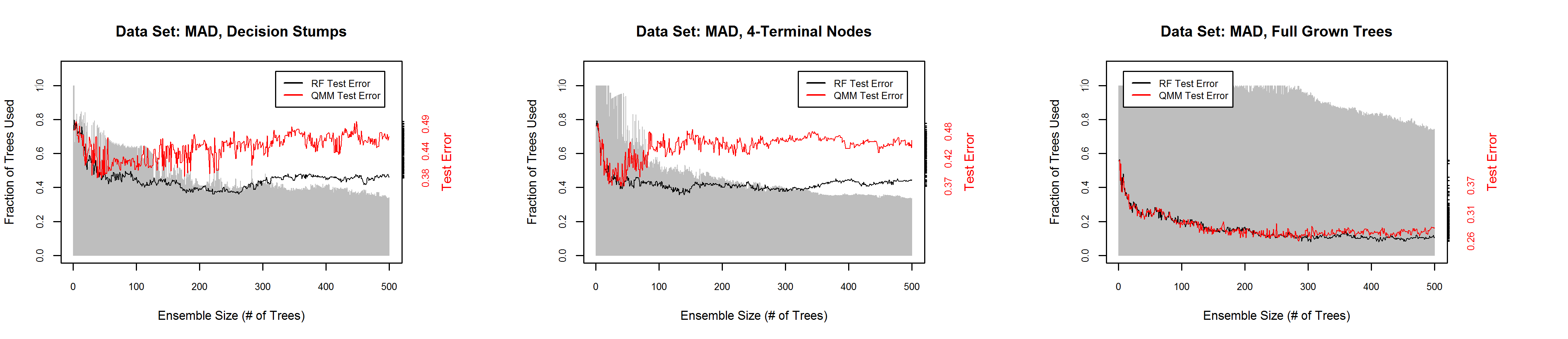
Figures 8, 9 and 10 show how the QMM algorithm compares to random forest ensembles for low, mid and high dimensional data sets using ensembles of size $T=1,2,...,500$. We can see the fraction of weak learners used in the QMM algorithm is also on average decreasing as $T$ increases, and the performance is similar to the results using AdaBoost ensembles. For low dimensional data sets the QMM algorithm uses on average 17, 57.2 and 216 trees out of 500 for decision stumps, 4-node trees and full-grown trees respectively. The average tree sizes for the QMM algorithm are 31.2, 97.6 and 186.8 for decision stumps, 4-node trees and full-grown trees respectively for mid dimensional data sets, and 119.3, 202.7 and 273.7 for high dimensional data sets. The QMM algorithm is able to produce significant improvements to the random forest solutions in some data sets, however it does perform worse in others. On average, though, the QMM algorithm does provide improvements both in the test set error and the reduction in the size of the ensemble compared to the random forest solutions.

Table 3: Description of Data Sets (High Dimensional)

Data Set	Description	Source	Train	Test	Features
CC	Colon Cancer Data	Alon et al. (1999)	43	19	2000
GIS	Digit Recognition Data	Guyon et al. (2004)	6000	1000	5000
MAD	Artificial Data	Guyon et al. (2004)	2000	600	500

5.2 QMM Performance Under Noise

Ensembles, particularly AdaBoost, tend to be sensitive to outliers and noise. Grove and Schuurmans (1998), Mason et al. (2000) and Dietterich (2000) provide evidence that AdaBoost does overfit and the generalization error deteriorates rapidly when the data is noisy. Long and Servedio (2010) proved that for any boosting algorithm with a potential convex loss function, and any nonzero random classification noise rate, there is a data set, which can be efficiently learnable by the booster if there is no noise, but cannot be learned with accuracy better than 1/2 with random classification noise present. Many methods that automatically handle noisy data and outliers have been proposed to alleviate the limitations of AdaBoost. Algorithms such as BrownBoost (Freund, 2001), LogitBoost (Friedman et al., 2000), MadaBoost (Domingo and Watanabe, 2000), LPReg-AdaBoost (Rätsch et al., 2001), $\nu$-LP and $\nu$-ARC, (Rätsch, 2001) mostly attempt to accommodate noise by somehow allowing unusual observations to fall in on the wrong side of the prediction in subsequent iterations of AdaBoost. Although bagging and random forests generally perform better than AdaBoost under noisy circumstances, they are still not completely robust to noise and outliers (Maclin and Opitz, 1997). Deleting outliers (also called noise filtering or noise peeling) by pre-processing the data is preferable under certain high noise circumstances (Martinez and Gray, 2016).

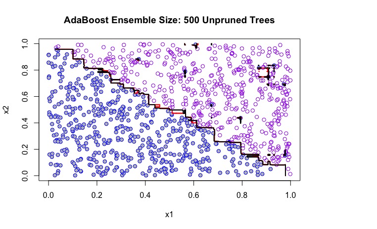
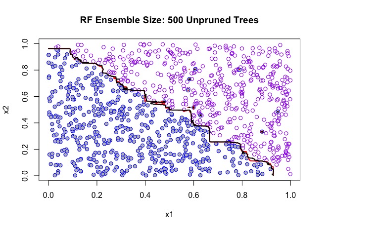
To visually illustrate how the QMM algorithm performs under a noisy scenario, we generate a synthetic two dimensional data set consisting of 1000 data points uniformly distributed on the unit square with $y=-1$ when $x1+x2<1$, and $y=+1$ when $x1+x2>1$, and randomly assign to $y\in\{-1,1\}$, when $x1+x2=1$. The true boundary would be the diagonal line $x1+x2=1$. To generate noise, we randomfly flip the response variable of 20 observations with $y=-1$ to $y=+1$. A test set of 1000 observations with no noise was also generated to gauge upon the performance of the methods. Figure 4 shows the decision boundaries for AdaBoost and Random Forests and the corresponding solutions for the QMM algorithm using 500 full-grown trees. The QMM algorithm improves slightly upon the performance of AdaBoost, since it is evident that it does overfit the data set by trying to more closely get a boundary for the noisy points. The random forest solution does not overfit as closely, but its boundary looks more ragged than that of AdaBoost.

(a)

(b)

Figure 4: Performance of the QMM algorithm with $\upsilon=0.5$ for AdaBoost and Random Forest using full-grown trees. The test set error for AdaBoost is 0.0280, compared to 0.0240 for the QMM algorithm, pruning the ensemble to only 127 trees. The RF test error rate was 0.0228 compared to QMM test error of 0.0224 selecting only 165 trees.

(a)

(b)

(c)

(d)

(e)

Figure 5: Performance of the QMM algorithm vs. AdaBoost for low dimensional data sets using $\upsilon=0.5$. The shaded grey represents the fraction of weak learners used given the ensemble size, while the red and black curves represent the test set error rates of the QMM algorithm and AdaBoost respectively.

(a)

(b)

(c)

(d)

(e)

Figure 6: Performance of the QMM algorithm vs. AdaBoost for mid dimensional data sets using $\upsilon=0.5$. The shaded grey represents the fraction of weak learners used given the ensemble size, while the red and black curves represent the test set error rates of the QMM algorithm and AdaBoost respectively.

(a)

(b)

(c)

Figure 7: Performance of the QMM algorithm vs. AdaBoost for high dimensional data sets using $\upsilon=0.5$. The shaded grey represents the fraction of weak learners used given the ensemble size, while the red and black curves represent the test set error rates of the QMM algorithm and AdaBoost respectively.

(a)

(b)

(c)

(d)

(e)

Figure 8: Performance of the QMM algorithm vs. random forests for low dimensional data sets using $\upsilon=0.25$. The shaded grey represents the fraction of weak learners used given the ensemble size, while the red and black curves represent the test set error rates of the QMM algorithm and AdaBoost respectively.

(a)

(b)

(c)

(d)

(e)

Figure 9: Performance of the QMM algorithm vs. random forests for mid dimensional data sets using $\upsilon=0.25$. The shaded grey represents the fraction of weak learners used given the ensemble size, while the red and black curves represent the test set error rates of the QMM algorithm and AdaBoost respectively.

(a)

(b)

(c)

Figure 10: Performance of the QMM algorithm vs. random forests for high dimensional data sets using $\upsilon=0.25$. The shaded grey represents the fraction of weak learners used given the ensemble size, while the red and black curves represent the test set error rates of the QMM algorithm and AdaBoost respectively.

5.3 Comparison to Other Ensemble Pruning Methodologies

We test how the proposed method compares to two of the leading ensemble pruning techniques: the Diversity Regularized Ensemble Pruning (DREP) method (Li et al., 2012) and $\kappa$-pruning (Margineantu and Dietterich, 1997). Both are selection-based methods and considered to be two of the leading ensemble pruning algorithms. One of the main drawbacks of ordered-ensemble pruning methods such as $\kappa$-pruning, is that we need to specify the size of the pruned subensemble and it might not necessarily be the optimal size. Several authors have considered that pruning close to 80% of a given ensemble yields the most consistent good results. For that particular reason, we set the $\kappa$-pruning method to prune 80% of the given ensemble. We show the test set error rate, the resulting ensemble size, along with a measure of diversity of the method. In this research we define diversity as:

$$\text{div}(f)=1-\frac{1}{\sum_{1\leq i\neq j\leq T}1}\sum_{1\leq i\neq j\leq T}\text{diff}(h_{i},h_{j}).$$ (25)

where $\text{diff}(h_{i},h_{j})=1/n\sum_{k=1}^{n}I[h_{i}(\textbf{x}_{k})h_{j}(\textbf{x}_{k})<0]$.

Table 4: Summary for AdaBoost Ensembles. Test Error Average Rank and Average Pruning Rate.

	Decision Stumps		4-Node Trees		Full-Grown Trees
	Test Error Rank	Pruning Rate	Test Error Rank	Pruning Rate	Test Error Rank	Pruning Rate
AdaBoost	1.31		1.46		1.69
QMM	1.08	0.9229	1.46	0.7900	1.54	0.6417
DREP	3.23	0.9758	2.77	0.8943	2.92	0.9518
$\kappa$-pruning	3.69	0.8000	3.46	0.8000	2.07	0.8000

Tables 6, 7 and 8 summarize the comparison results for AdaBoost ensembles. The simulations suggest that DREP prunes trees more aggresively than both the QMM algorithm and $\kappa$-pruning, however the QMM algorithm performs better in terms of the test set error in most of the cases, which is not surprising given the primary emphasis of the algorithm to achieve better performance, as opposed to explicitly prune the ensemble. For low dimensional data sets the QMM algorithm performs very similar to the original AdaBoost ensemble in terms of the test set error, but only using around 12% of the trees generated by the AdaBoost solution. Table 4 is a breakdown of the average rank of the test error rates for the methods compared, along with the average pruning rate for AdaBoost solutions. In terms of generalization error performance, the average rank of the QMM algorithm is 1.08, 1.46, and 1.54 for decision stumps, 4-node (depth = 2) trees and full-grown trees respective. The QMM algorithm ranks better than DREP and $\kappa$-pruning for decision stumps, 4-node (depth = 2) and full grown trees, and ranks on average better than the original AdaBoost solution for decision stumps and full-grown trees, with a tied performance on 4-node trees. The average pruning rate for the QMM is 92.29% for decision stumps, 79% for 4-node trees and 64.17% for full-grown trees. DREP on average prunes the trees more aggresively than the QMM algorithm with an average pruning rate of 97.58% for decision stumps, 89.43% for 4-node trees and 95.18% for full-grown trees. Tables 9, 10 and 11 show the comparison results for Random Forest ensembles. For Random Forest solutions, the QMM algorithm ranks best on average in terms of generalization performance for both decision stumps and 4-node (depth = 2) trees, while it ranks second in full-grown trees after the original Random Forest solution. $\kappa$-pruning outperforms DREP only in full-grown trees. In terms of the pruning rate, DREP also obtains on average a higher pruning rate under all decision tree types.

Table 5: Summary for Random Forest Ensembles. Test Error Average Rank and Average Pruning Rate.

	Decision Stumps		4-Node Trees		Full-Grown Trees
	Test Error Rank	Pruning Rate	Test Error Rank	Pruning Rate	Test Error Rank	Pruning Rate
Random Forest	2.46		1.85		1.84
QMM	1.69	0.9078	1.62	0.7874	2.08	0.5638
DREP	2.08	0.9263	2.46	0.9245	3.15	0.9637
$\kappa$-pruning	2.83	0.8000	3.15	0.8000	2.77	0.8000

6 Conclusions and Future Research

Ensembles generally perform strongly in terms of their generalization ability compared to individual classifiers. The proliferation of large scale, high velocity data sets, often containing variables of different data types, creates challenges for the use of ensembles in industry. Recent research effort has concentrated in reducing the size of ensembles, while maintaining their predictive accuracy (pruning the ensemble). In this paper, we propose a quadratic program formulation that aims to tune the weights of a given ensemble, such that the pairwise correlations of the weak learners and the variance of the margin instances are minimized, while maximizing the lower percentiles of the margins. The proposed method results in a combined classifier with an average pruning rate of 91.5% for decision stumps, 78.9% for 4-node trees and 61.8% for full-grown trees. The generalization performance of the proposed method (the QMM algorithm) compares favorably to that of the original ensemble and other ensemble pruning methodologies analyzed here. Moreover, the proposed method, as with many ensemble pruning methodologies, appears to offer some improvements over the original ensemble in data sets containing noisy examples. Further directions for this research include to implicitly adhere cost functions in the boosting and random forest ensembles that maximize the lower margin distribution and select the most diverse classifiers.

Table 6: Comparison of the QMM Algorithm to Existing Methodologies in Low Dimensional Data Sets (AdaBoost Solutions).

		500 Trees (decision stumps)			500 Trees (4-terminal nodes)			500 Trees (full-grown)
		Test Error	Ensemble Size	Diversity	Test Error	Ensemble Size	Diversity	Test Error	Ensemble Size	Diversity
AU	AdaBoost	0.1202	500	0.51818	0.1105	500	0.52969	0.1009	500	0.67624
	QMM	0.1202	22	0.99923	0.1105	67	0.98555	0.1009	155	0.67624
	DREP	0.1346	1	1.00000	0.1058	27	0.99873	0.1250	17	0.99973
	$\kappa$-pruning	0.3894	100	0.99099	0.1298	100	0.98446	0.1154	100	0.98560
BAN	AdaBoost	0.3086	500	0.50273	0.2502	500	0.50863	0.1075	500	0.35591
	QMM	0.3061	17	0.99890	0.2357	19	0.99618	0.1068	71	0.99170
	DREP	0.3702	7	0.99998	0.2809	29	0.99835	0.1339	29	0.99779
	$\kappa$-pruning	0.3130	100	0.99636	0.2778	100	0.98157	0.2998	100	0.96775
BC	AdatBoost	0.0146	500	0.54122	0.0049	500	0.58258	0.0098	500	0.86199
	QMM	0.0146	28	0.99899	0.0049	55	0.98027	0.0098	98	0.94103
	DREP	0.0537	5	0.99999	0.0098	37	0.99814	0.0195	11	0.99996
	$\kappa$-pruning	0.0342	100	0.99151	0.0146	100	0.98788	0.0146	100	0.99299
DIA	AdaBoost	0.2468	500	0.53804	0.2468	500	0.54749	0.2641	500	0.60059
	QMM	0.2468	30	0.99845	0.2641	38	0.99175	0.2511	211	0.65181
	DREP	0.2641	5	0.99996	0.2337	26	0.99890	0.2641	38	0.99802
	$\kappa$-pruning	0.3550	100	0.98450	0.2597	100	0.98312	0.2511	100	0.98399
FC	AdaBoost	0.2124	500	0.54855	0.0232	500	0.57073	0.0232	500	0.98695
	QMM	0.2124	13	0.99971	0.0541	22	0.99441	0.0232	65	0.99906
	DREP	0.3320	3	0.99999	0.2625	23	0.99925	0.0232	3	1.00000
	$\kappa$-pruning	0.4285	100	0.99382	0.1737	100	0.98305	0.0232	100	0.99810

Table 7: Comparison of the QMM Algorithm to Existing Methodologies in Mid Dimensional Data Sets (AdaBoost Solutions).

		500 Trees (decision stumps)			500 Trees (4-terminal nodes)			500 Trees (full-grown)
		Test Error	Ensemble Size	Diversity	Test Error	Ensemble Size	Diversity	Test Error	Ensemble Size	Diversity
IJC	AdaBoost	0.1040	500	0.52748	0.0959	500	0.54184	0.0740	500	0.87387
	QMM	0.1040	75	0.99047	0.0935	242	0.89703	0.0740	96	0.99209
	DREP	0.0959	2	1.00000	0.1107	148	0.96062	0.0972	15	0.98352
	$\kappa$-pruning	0.3393	100	0.98360	0.1162	100	0.98295	0.0699	100	0.99640
ION	AdaBoost	0.0472	500	0.52661	0.0566	500	0.56099	0.0472	500	0.76899
	QMM	0.0472	24	0.99921	0.0566	76	0.95103	0.0472	244	0.94753
	DREP	0.1132	20	0.99927	0.0660	7	0.99994	0.1132	6	0.99999
	$\kappa$-pruning	0.1981	100	0.99087	0.3585	100	0.98245	0.0377	100	0.98810
MR	AdatBoost	0.0029	500	0.54464	0.0012	500	0.58310	0.0000	500	0.99985
	QMM	0.0029	14	0.99955	0.0000	37	0.99778	0.0000	8	1.00000
	DREP	0.1148	1	1.00000	0.0066	10	0.99988	0.0000	2	1.00000
	$\kappa$-pruning	0.0849	100	0.98607	0.0221	100	0.99393	0.0000	100	0.99997
SON	AdaBoost	0.1746	500	0.51665	0.1587	500	0.54364	0.1587	500	0.59817
	QMM	0.1429	51	0.99088	0.1587	145	0.96215	0.2222	145	0.96701
	DREP	0.2381	68	0.99124	0.2222	26	0.99884	0.2381	10	0.99988
	$\kappa$-pruning	0.3175	100	0.98168	0.1746	100	0.981742	0.1905	100	0.98273
SPL	AdaBoost	0.0662	500	0.52568	0.0359	500	0.55834	0.0359	500	0.76731
	QMM	0.0662	25	0.99883	0.0349	170	0.94612	0.0363	255	0.76731
	DREP	0.1651	42	0.99674	0.0446	103	0.98297	0.0556	4	1.00000
	$\kappa$-pruning	0.3402	100	0.98732	0.1582	100	0.98480	0.0363	100	0.99010

Table 8: Comparison of the QMM Algorithm to Existing Methodologies in High Dimensional Data Sets (AdaBoost Solutions).

		500 Trees (decision stumps)			500 Trees (4-terminal nodes)			500 Trees (full-grown)
		Test Error	Ensemble Size	Diversity	Test Error	Ensemble Size	Diversity	Test Error	Ensemble Size	Diversity
CC	AdaBoost	0.2105	500	0.62274	0.3684	500	0.00000	0.3684	500	0.59920
	QMM	0.2105	29	0.99814	0.3684	1	1.00000	0.3158	42	0.99770
	DREP	0.4210	1	1.00000	0.3684	1	1.00000	0.4210	2	0.99999
	$\kappa$-pruning	0.2631	100	0.98365	0.3684	100	0.96032	0.3158	100	0.99132
GIS	AdaBoost	0.0540	500	0.94414	0.0320	500	0.93792	0.0200	500	0.52574
	QMM	0.0540	135	0.99469	0.0320	325	0.95839	0.0200	465	0.52574
	DREP	0.1690	1	1.00000	0.0390	177	0.98646	0.0210	177	0.93672
	$\kappa$-pruning	0.1400	100	0.99093	0.0720	100	0.99364	0.0210	100	0.98647
MAD	AdaBoost	0.3783	500	0.50401	0.2933	500	0.50689	0.1783	500	0.52150
	QMM	0.3700	38	0.99660	0.3200	168	0.94464	0.1683	474	0.52150
	DREP	0.3883	1	1.00000	0.3450	87	0.99998	0.1967	75	0.98963
	$\kappa$-pruning	0.4400	100	0.98085	0.3266	100	0.98296	0.2250	100	0.98056

Table 9: Comparison of the QMM Algorithm to Existing Methodologies in Low Dimensional Data Sets (Random Forest Solutions).

		500 Trees (decision stumps)			500 Trees (4-terminal nodes)			500 Trees (full-grown)
		Test Error	Ensemble Size	Diversity	Test Error	Ensemble Size	Diversity	Test Error	Ensemble Size	Diversity
AU	RF	0.1442	500	0.68613	0.1105	500	0.73518	0.0961	500	0.75578
	QMM	0.1250	32	0.99819	0.1442	102	0.96848	0.0913	282	0.77948
	DREP	0.1250	51	0.99692	0.1106	52	0.99734	0.1250	18	0.99968
	$\kappa$-pruning	0.2500	100	0.98616	0.1538	100	0.98897	0.0961	100	0.98832
BAN	RF	0.3243	500	0.69109	0.3494	500	0.76218	0.1068	500	0.87735
	QMM	0.3193	4	0.99997	0.2099	14	0.99962	0.1081	470	0.87735
	DREP	0.4192	11	0.99985	0.3620	3	0.99999	0.1087	45	0.99903
	$\kappa$-pruning	0.4173	100	0.99643	0.4028	100	0.99145	0.1119	100	0.99460
BC	RF	0.0292	500	0.90661	0.0098	500	0.93904	0.0098	500	0.94265
	QMM	0.0146	14	0.99988	0.0098	34	0.99964	0.0146	15	0.99993
	DREP	0.0292	9	0.99997	0.0098	11	0.99998	0.0341	4	1.00000
	$\kappa$-pruning	0.0376	100	0.99615	0.0195	100	0.99613	0.0146	100	0.99697
DIA	RF	0.2510	500	0.67500	0.2640	500	0.71681	0.2467	500	0.67500
	QMM	0.2641	31	0.67641	0.2554	126	0.94086	0.2511	300	0.67632
	DREP	0.2554	58	0.99969	0.2554	51	0.99695	0.2640	16	0.99969
	$\kappa$-pruning	0.3246	100	0.98610	0.2727	100	0.99068	0.2554	100	0.98610
FC	RF	0.3359	500	0.71945	0.2007	500	0.78693	0.0116	500	0.91949
	QMM	0.2432	4	0.99998	0.1737	10	0.99985	0.0309	13	0.99992
	DREP	0.2780	4	0.99589	0.2896	9	0.99995	0.0232	5	0.99999
	$\kappa$-pruning	0.3243	100	0.99711	0.2278	100	0.99766	0.0154	100	0.99535

Table 10: Comparison of the QMM Algorithm to Existing Methodologies in Mid Dimensional Data Sets (Random Forest Solutions).

		500 Trees (decision stumps)			500 Trees (4-terminal nodes)			500 Trees (full-grown)
		Test Error	Ensemble Size	Diversity	Test Error	Ensemble Size	Diversity	Test Error	Ensemble Size	Diversity
IJC	RF	0.0959	500	1.00000	0.0959	500	0.99130	0.0520	500	0.32555
	QMM	0.0959	12	1.00000	0.0959	70	0.99968	0.0522	367	0.328200
	DREP	0.0959	3	1.00000	0.0959	4	1.00000	0.0555	59	0.99091
	$\kappa$-pruning	0.0959	100	1.00000	0.0959	100	0.99867	0.0466	100	0.97544
ION	RF	0.2358	500	0.50635	0.0377	500	0.77674	0.0566	500	0.81124
	QMM	0.1887	32	0.99579	0.0472	96	0.97949	0.0377	111	0.97477
	DREP	0.2358	2	0.99999	0.0755	13	0.99987	0.0471	7	0.99997
	$\kappa$-pruning	0.2170	100	0.98236	0.1132	100	0.99065	0.0471	100	0.99069
MR	RF	0.1095	500	0.70385	0.0890	500	0.77811	0.0000	500	0.99164
	QMM	0.0689	31	0.99947	0.0422	68	0.99181	0.0037	1	1.00000
	DREP	0.1140	3	0.99999	0.0972	11	0.99993	0.0008	2	1.00000
	$\kappa$-pruning	0.2506	100	0.98546	0.1058	100	0.98800	0.0000	100	0.99928
SON	RF	0.2698	500	0.85220	0.2698	500	0.79122	0.2222	500	0.79578
	QMM	0.2539	40	0.99893	0.2857	82	0.98355	0.1587	99	0.98402
	DREP	0.2063	35	0.99919	0.2857	13	0.99986	0.1905	6	0.99998
	$\kappa$-pruning	0.1905	100	0.99469	0.2063	100	0.99513	0.2381	100	0.99513
SPL	RF	0.1678	500	0.84542	0.0869	500	0.79140	0.0285	500	0.62272
	QMM	0.1264	41	0.99926	0.0483	172	0.96441	0.0280	356	0.62272
	DREP	0.1651	91	0.99556	0.0993	119	0.98794	0.0662	13	0.99976
	$\kappa$-pruning	0.3457	100	0.99035	0.1660	100	0.99334	0.0303	100	0.98926

Table 11: Comparison of the QMM Algorithm to Existing Methodologies in High Dimensional Data Sets (Random Forest Solutions).

		500 Trees (decision stumps)			500 Trees (4-terminal nodes)			500 Trees (full-grown)
		Test Error	Ensemble Size	Diversity	Test Error	Ensemble Size	Diversity	Test Error	Ensemble Size	Diversity
CC	AdaBoost	0.2631	500	0.72614	0.3684	500	0.69650	0.3684	500	0.70117
	QMM	0.3158	27	0.99822	0.1579	33	0.99808	0.3684	29	0.99843
	DREP	0.3158	8	0.99995	0.2105	2	0.99999	0.2105	4	0.99997
	$\kappa$-pruning	0.1579	100	0.99558	0.2632	100	0.99394	0.2631	100	0.99366
GIS	AdaBoost	0.2810	500	0.71720	0.1260	500	0.74891	0.0320	500	0.84613
	QMM	0.1060	109	0.96065	0.1040	285	0.81060	0.0310	358	0.84613
	DREP	0.2770	13	0.99984	0.1320	190	0.96449	0.0340	25	0.99963
	$\kappa$-pruning	0.3410	100	0.98808	0.1750	100	0.98848	0.0340	100	0.99314
MAD	AdatBoost	0.3883	500	0.95258	0.3800	500	0.92124	0.2650	500	0.96271
	QMM	0.4550	222	0.99895	0.4417	290	0.96039	0.2967	434	0.96296
	DREP	0.3683	191	0.99221	0.4167	13	0.99991	0.3250	32	0.99984
	$\kappa$-pruning	0.3850	100	0.99071	0.3800	100	0.99353	0.3267	100	0.99922

References

- Alon et al. (1999) Uri Alon, Naama Barkai, Daniel A Notterman, Kurt Gish, Suzanne Ybarra, Daniel Mack, and Arnold J Levine. Broad patterns of gene expression revealed by clustering analysis of tumor and normal colon tissues probed by oligonucleotide arrays. Proceedings of the National Academy of Sciences, 96(12):6745–6750, 1999.
- Banfield et al. (2003) Robert E. Banfield, Lawrence O. Hall, Kevin W. Bowyer, and W. Philip Kegelmeyer. A new ensemble diversity measure applied to thinning ensembles. Multiple Classifier Systems, pages 306–316, 2003.
- Banfield et al. (2005) Robert E. Banfield, Lawrence O. Hall, Kevin W. Bowyer, and W. Philip Kegelmeyer. Ensemble diversity measures and their application to thinning. Information Fusion, 6(1):49–62, 2005.
- Blaser and Fryzlewicz (2016) Rico Blaser and Piotr Fryzlewicz. Random rotation forests. The Journal of Machine Learning Research, 17:1–26, 2016.
- Breiman (1996a) Leo Breiman. Bagging predictors. Machine Learning, 24(2):123–140, 1996a.
- Breiman (1996b) Leo Breiman. Bias, variance, and arcing classifiers. Technical Report 460, 1996b.
- Breiman (1999) Leo Breiman. Prediction games and arcing algorithms. Neural Computation, 11(7):1493–1517, 1999.
- Breiman (2001) Leo Breiman. Random forests. Machine Learning, 45(1):5–32, 2001.
- Breiman et al. (1984) Leo Breiman, Jerome Friedman, Charles J Stone, and Richard A Olshen. Classification and regression trees. CRC press, 1984.
- Brown et al. (2005) Gavin Brown, Jeremy L Wyatt, and Peter Tiňo. Managing diversity in regression ensembles. Journal of Machine Learning Research, 6(Sep):1621–1650, 2005.
- Chen et al. (2006) Huanhuan Chen, Peter Tino, and Xin Yao. A probabilistic ensemble pruning algorithm. In Sixth IEEE International Conference on Data Mining-Workshops (ICDMW’06), pages 878–882. IEEE, 2006.
- Chen et al. (2009) Huanhuan Chen, Peter Tiho, and Xin Yao. Predictive ensemble pruning by expectation propagation. Knowledge and Data Engineering, IEEE Transactions on, 21(7):999–1013, 2009.
- Cid (2012) Waldyn Gerardo Martinez Cid. Three essays on the use of margins to improve ensemble models. PhD thesis, The University of Alabama, 2012.
- Cortes and Vapnik (1995) Corinna Cortes and Vladimir Vapnik. Support-vector networks. Machine Learning, 20(3):273–297, 1995.
- Cover and Thomas (1991) Thomas M. Cover and Joy A. Thomas. Information theory and statistics. Elements of Information Theory, pages 279–335, 1991.
- Dai (2013) Qun Dai. A competitive ensemble pruning approach based on cross-validation technique. Knowledge-Based Systems, 37:394–414, 2013.
- Demiriz et al. (2002) Ayhan Demiriz, Kristin P Bennett, and John Shawe-Taylor. Linear programming boosting via column generation. Machine Learning, 46(1-3):225–254, 2002.
- Dietterich (2000) Thomas G. Dietterich. Ensemble methods in machine learning. Multiple Classifier Systems, pages 1–15, 2000.
- Domingo and Watanabe (2000) Carlos Domingo and Osamu Watanabe. Madaboost: A modification of adaboost. COLT, pages 180–189, 2000.
- Drucker et al. (1994) Harris Drucker, Corinna Cortes, Lawrence D. Jackel, Yann LeCun, and Vladimir Vapnik. Boosting and other ensemble methods. Neural Computation, 6(6):1289–1301, 1994.
- Freund (2001) Yoav Freund. An adaptive version of the boost by majority algorithm. Machine learning, 43(3):293–318, 2001.
- Freund and Schapire (1997) Yoav Freund and Robert E. Schapire. A decision-theoretic generalization of on-line learning and an application to boosting. Journal of Computer and System Sciences, 55:119–139, 1997.
- Friedman (2001) Jerome H. Friedman. Greedy function approximation: a gradient boosting machine. Annals of statistics, pages 1189–1232, 2001.
- Friedman (2002) Jerome H. Friedman. Stochastic gradient boosting. Computational Statistics and Data Analysis, 38(4):367–378, 2002.
- Friedman et al. (2000) Jerome H. Friedman, Trevor Hastie, Robert Tibshirani, et al. Additive logistic regression: a statistical view of boosting (with discussion and a rejoinder by the authors). Annals of Statistics, 28(2):337–407, 2000.
- Gao and Zhou (2013) Wei Gao and Zhi-Hua Zhou. On the doubt about margin explanation of boosting. Artificial Intelligence, 203:1–18, 2013.
- Germain et al. (2015) Pascal Germain, Alexandre Lacasse, François Laviolette, Mario Marchand, and Jean-Francis Roy. Risk bounds for the majority vote: From a pac-bayesian analysis to a learning algorithm. The Journal of Machine Learning Research, 16(1):787–860, 2015.
- Grove and Schuurmans (1998) Adam J. Grove and Dale Schuurmans. Boosting in the limit: Maximizing the margin of learned ensembles. Proceedings of the Fifteenth National Conference on Artificial Intelligence, pages 692–699, 1998.
- Guo and Boukir (2013) Li Guo and Samia Boukir. Margin-based ordered aggregation for ensemble pruning. Pattern Recognition Letters, 34(6):603–609, 2013.
- Guyon et al. (2004) Isabelle Guyon, Steve Gunn, Asa Ben-Hur, and Gideon Dror. Result analysis of the nips 2003 feature selection challenge. In Advances in neural information processing systems, pages 545–552, 2004.
- Ho and Kleinberg (1996) Tin Kam Ho and Eugene M Kleinberg. Building projectable classifiers of arbitrary complexity. In Pattern Recognition, 1996., Proceedings of the 13th International Conference on, volume 2, pages 880–885. IEEE, 1996.
- Kearns and Valiant (1994) Michael Kearns and Leslie Valiant. Cryptographic limitations on learning boolean formulae and finite automata. Journal of the ACM (JACM), 41(1):67–95, 1994.
- Kohen (1960) Jacob Kohen. A coefficient of agreement for nominal scale. Educational and Psychological Measurements, 20:37–46, 1960.
- Kuncheva and Hadjitodorov (2004) Ludmila I. Kuncheva and Stefan T. Hadjitodorov. Using diversity in cluster ensembles. Systems, Man and Cybernetics, 2004 IEEE international Conference on, 2:1214–1219, 2004.
- Kuncheva and Whitaker (2003) Ludmila I. Kuncheva and Christopher J. Whitaker. Measures of diversity in classifier ensembles and their relationship with the ensemble accuracy. Machine learning, 51(2):181–207, 2003.
- Li et al. (2012) Nan Li, Yang Yu, and Zhi-Hua Zhou. Diversity regularized ensemble pruning. Machine Learning and Knowledge Discovery in Databases, pages 330–345, 2012.
- Lichman (2013) M. Lichman. UCI machine learning repository, 2013. URL http://archive.ics.uci.edu/ml.
- Liu et al. (2004) Huan Liu, Amit Mandvikar, and Jigar Mody. An empirical study of building compact ensembles. Advances in Web-Age Information Management, pages 622–627, 2004.
- Long and Servedio (2010) Philip M Long and Rocco A Servedio. Random classification noise defeats all convex potential boosters. Machine Learning, 78(3):287–304, 2010.
- Lu et al. (2010) Zhenyu Lu, Xindong Wu, Xingquan Zhu, and Josh Bongard. Ensemble pruning via individual contribution ordering. Proceedings of the 16th ACM SIGKDD international conference on Knowledge discovery and data mining, pages 871–880, 2010.
- Ma et al. (2015) Zhongchen Ma, Qun Dai, and Ningzhong Liu. Several novel evaluation measures for rank-based ensemble pruning with applications to time series prediction. Expert Systems with Applications, 42(1):280–292, 2015.
- Maclin and Opitz (1997) Richard Maclin and David Opitz. An empirical evaluation of bagging and boosting. AAAI/IAAI, 1997:546–551, 1997.
- Maclin and Opitz (2011) Richard Maclin and David Opitz. Popular ensemble methods: An empirical study. Journal of Artificial Intelligence Research, 11:169–198, 2011.
- Margineantu and Dietterich (1997) Dragos D. Margineantu and Thomas G. Dietterich. Pruning adaptive boosting. ICML, 97:211–218, 1997.
- Martinez and Gray (2014) Waldyn Martinez and J. Brian Gray. The role of margins in boosting and ensemble performance. Wiley Interdisciplinary Reviews: Computational Statistics, 6(2):124–131, 2014.
- Martinez and Gray (2016) Waldyn Martinez and J. Brian Gray. Noise peeling methods to improve boosting algorithms. Computational Statistics & Data Analysis, 93:483–497, 2016.
- Martinez-Munoz and Suarez (2006) Gonzalo Martinez-Munoz and Alberto Suarez. Pruning in ordered bagging ensembles. In Proceedings of the 23rd international conference on Machine learning, pages 609–616. ACM, 2006.
- Martinez-Munoz et al. (2009) Gonzalo Martinez-Munoz, Daniel Hernandez-Lobato, and Almudena Suarez. An analysis of ensemble pruning techniques based on ordered aggregation. Pattern Analysis and Machine Intelligence, IEEE Transactions on, 31(2):245–259, 2009.
- Mason et al. (2000) Llew Mason, Peter L. Bartlett, and Jonathan Baxter. Improved generalization through explicit optimization of margins. Machine Learning, 38(3):243–255, 2000.
- Megahed and Jones-Farmer (2013) Fadel M. Megahed and L. Allison Jones-Farmer. A statistical process monitoring perspective on big data. Frontiers in Statistical Quality Control, 11th ed. Springer, New York, 2013.
- Opitz and Maclin (1999) David Opitz and Richard Maclin. Popular ensemble methods: An empirical study. Journal of Artificial Intelligence Research, pages 169–198, 1999.
- Partalas et al. (2006) Loannis Partalas, Grigorios Tsoumakas, Loannis Katakis, and Loannis Vlahavas. Ensemble pruning using reinforcement learning. Advances in Artificial Intelligence, pages 301–310, 2006.
- Prodromidis and Stolfo (2001) Andreas L Prodromidis and Salvatore J Stolfo. Cost complexity-based pruning of ensemble classifiers. Knowledge and Information Systems, 3(4):449–469, 2001.
- Prokhorov (2001) Danil Prokhorov. Slide presentation in ijcnn’01, ford research laboratory. IJCNN, 2001.
- Quinlan (1996) J. Ross Quinlan. Bagging, boosting, and c4. 5. AAAI/IAAI, Vol. 1, pages 725–730, 1996.
- Rätsch (2001) Gunnar Rätsch. Robust boosting via convex optimization: Theory and applications, 2001.
- Rätsch (2014) Gunnar Rätsch. Ida benchmark repository. https://mldata.org/, 2014.
- Rätsch et al. (2001) Gunnar Rätsch, Takashi Onoda, and K-R Müller. Soft margins for adaboost. Machine learning, 42(3):287–320, 2001.
- Reyzin and Schapire (2006) Lev Reyzin and Robert E. Schapire. How boosting the margin can also boost classifier complexity. Proceedings of the 23rd international conference on Machine learning, pages 753–760, 2006.
- Rodriguez et al. (2006) Juan J. Rodriguez, Ludmila I. Kuncheva, and Carlos J. Alonso. Rotation forest: A new classifier ensemble method. Pattern Analysis and Machine Intelligence, IEEE Transactions on, 28(10):1619–1630, 2006.
- Schapire (1990) Robert E. Schapire. The strength of weak learnability. Machine learning, 5(2):197–227, 1990.
- Schapire (1999) Robert E. Schapire. Theoretical views of boosting. Computational Learning Theory, pages 1–10, 1999.
- Schapire et al. (1998) Robert E. Schapire, Yoav Freund, Peter Bartlett, and Wee S. Lee. Boosting the margin: A new explanation for the effectiveness of voting methods. Annals of Statistics, 26:1651–1686, 1998.
- Seiffert et al. (2008) Chris Seiffert, Taghi M Khoshgoftaar, Jason Van Hulse, and Amri Napolitano. Resampling or reweighting: A comparison of boosting implementations. In Tools with Artificial Intelligence, 2008. ICTAI’08. 20th IEEE International Conference on, volume 1, pages 445–451. IEEE, 2008.
- Shen and Li (2010) Chunhua Shen and Hanxi Li. Boosting through optimization of margin distributions. Neural Networks, IEEE Transactions on, 21(4):659–666, 2010.
- Tsoumakas et al. (2009) Grigorios Tsoumakas, Loannis Partalas, and Loannis Vlahavas. An ensemble pruning primer. Applications of Supervised and Unsupervised Ensemble Methods, pages 1–13, 2009.
- Tsymbal et al. (2005) Alexey Tsymbal, Mykola Pechenizkiy, and Pádraig Cunningham. Diversity in search strategies for ensemble feature selection. Information fusion, 6(1):83–98, 2005.
- Valiant (1984) Leslie G. Valiant. A theory of the learnable. Communications of the ACM, 27(11):1134–1142, 1984.
- Wang et al. (2011) Liwei Wang, Masashi Sugiyama, Zhaoxiang Jing, Cheng Yang, Zhi-Hua Zhou, and Jufu Feng. A refined margin analysis for boosting algorithms via equilibrium margin. The Journal of Machine Learning Research, 12:1835–1863, 2011.
- Wang et al. (2012) Liwei Wang, Xiaocheng Deng, Zhaoxiang Jing, and JuFu Feng. Further results on the margin explanation of boosting: new algorithm and experiments. Science China Information Sciences, 55(7):1551–1562, 2012.
- Zhang and Zhang (2008) Chun-Xia Zhang and Jiang-She Zhang. A local boosting algorithm for solving classification problems. Computational Statistics and Data Analysis, 52(4):1928–1941, 2008.
- Zhang and Zhang (2009) Chun-Xia Zhang and Jiang-She Zhang. A novel method for constructing ensemble classifiers. Statistics and Computing, 19(3):317–327, 2009.
- Zhang et al. (2009) Jun Zhang, Kwok-Wing Chau, et al. Multilayer ensemble pruning via novel multi-sub-swarm particle swarm optimization. J. UCS, 15(4):840–858, 2009.
- Zhang et al. (2006) Yi Zhang, Samuel Burer, and W Nick Street. Ensemble pruning via semi-definite programming. The Journal of Machine Learning Research, 7:1315–1338, 2006.
- Zhou (2014) Zhi-Hua Zhou. Large margin distribution learning. Artificial Neural Networks in Pattern Recognition, pages 1–11, 2014.
- Zhou et al. (2002) Zhi-Hua Zhou, Jianxin Wu, and Wei Tang. Ensembling neural networks: many could be better than all. Artificial intelligence, 137(1):239–263, 2002.