Characterizing atomic magnetic gradiometers for fetal magnetocardiography

Abstract

Atomic magnetometers (AMs) offer many advantages over superconducting quantum interference devices (SQUIDs) due to, among other things, having comparable sensitivity while not requiring cryogenics. One of the major limitations of AMs is the challenge of configuring them as gradiometers. We report the development of a spin-exchange relaxation free (SERF) vector atomic magnetic gradiometer with sensitivity of $3\,\rm{fT}\,{cm}^{-1}{Hz}^{-1/2}$ and common mode rejection ratio (CMRR) $>150$ in the band from DC to 100 Hz. We introduce a background suppression figure of merit for characterizing the performance of gradiometers. It allows for optimally setting the measurement baseline, and for quickly assessing the advantage, if any, of performing a measurement in gradiometric mode. As an application, we consider the problem of fetal magnetocardiography (fMCG) detection in the presence of a large background maternal MCG signal.

I Introduction

Magnetic gradiometers can often achieve higher fidelity detection of localized magnetic field distributions than magnetometers. This is true in environments where the primary noise sources are far from the detectors such as in magnetocardiography (MCG), magnetoencephalography (MEG) Colombo et al. (2016); Sander et al. (2012), geomagnetism Keenan, Blay, and Romans (2011), ordnance detection Wiegert and Oeschger (2006) and in low field NMR Jiang et al. (2019), with the benefit arising with suppression of common mode noise. Sensitivity, bandwidth and dynamic range determine the optimal choice of sensor for each application.

Consider a situation where a uniform magnetic field $B_{c}$ component (or magnitude for scalar sensors) is measured by two closely separated sensors. The common mode rejection ratio, CMRR is

$$\xi=\frac{M_{1}B_{1c}+M_{2}B_{2c}}{2(M_{1}B_{1c}-M_{2}B_{2c})}=\frac{M_{1}+M_{2}}{2(M_{1}-M_{2})}$$ (1)

where $B_{ic}$ is the field measured by sensor $i$, and $M_{i}$ is the transfer function for each sensor. For identical sensors in this situation $(M_{1}=M_{2},B_{1c}=B_{2c})$, we expect a CMRR of infinity resulting in vanishing sensitivity to the difference signal. In practice however, differences in sensors lead to a finite CMRR $\xi$.

Presently, the highest performing magnetic gradiometers involve inductively coupling the magnetic field of interest to low Tc superconducting quantum interference devices, SQUIDs via counter-wound pickup coils Quartero et al. (2002); Strasburger, Cheulkar, and Wakai (2008). The SQUID gradiometer CMRR is limited by the degree to which the areas and alignments of these (often hand-wound) coils are matched. Typical values of SQUID gradiometer balance is about one part in 100, setting the upper bound of the common-mode suppression at that level. Hämäläinen et al. (1993); Clarke and Braginski (2009).

Unlike SQUIDs, atomic magnetometers (AMs) require no cryogens. They are relatively inexpensive to operate and have significantly lower setup and operating costs due to their working temperatures and smaller shielding volume requirements. However, configuring AMs as gradiometers poses a number of challenges and is an active area of work Affolderbach et al. (2002); Dang, Maloof, and Romalis (2010); Kominis et al. (2003); Kim et al. (2014); Kamada et al. (2015); Sheng et al. (2013, 2017); Johnson, Schwindt, and Weisend (2010); Xu et al. (2006).

Most AM gradiometer implementations, this work included, involve subtracting magnetic field measurements from adjacent sensors in post processing. In this paper, we consider the challenge of performing such a subtraction and recommend procedures for calibrating and characterizing AM gradiometers. In section II, we introduce a figure of merit for evaluating gradiometer performance. It is a function of the CMRR, the gradiometer baseline, as well as the geometric scaling of the signal and the dominant background fields. This metric will be useful for comparing different implementations of gradiometers when applying the sensors to a particular measurement problem. In section III, we report the development of Spin Exchange Relaxation Free (SERF) gradiometers with performance metrics comparable to SQUIDs. Finally, in section IV, we consider the problem of detecting fetal magneto-cardiography (fMCG) in the presence of the large maternal MCG signal. Our goal is to efficiently isolate the fMCG signal from the maternal background. Some relevant questions to address are how best to configure the sensors, what CMRR is sufficient and how to compare different gradiometer implementations. We shall discuss the gradiometer we have developed in comparisons with others in the literature.

II Gradiometry Figure of Merit

Often, measurements from an array of magnetic field sensors are input into an analysis pipeline for further processing: e.g for source localization, Independent Component Analysis etc. The question we consider is if and when does using the output of gradiometers provide an advantage over using magnetometers?

Consider a magnetic field signal described by the power law $B(r)\propto(1/r)^{p}$ in the presence of noise with rms amplitude $\delta B=(\delta B_{u}^{2}+\delta B_{c}^{2})^{1/2}$, where $\delta B_{u}$ and $\delta B_{c}$ are the rms magnitudes of uncorrelated and correlated (uniform) noise respectively. A gradiometric measurement of such a field is only beneficial if the signal-to-noise ratio in gradiometric mode is superior to that obtained from two separate magnetometers. We therefore define a figure of merit $\mathcal{F}$ as the ratio:

$$\mathcal{F}=\frac{SNR_{G}}{SNR_{M}} =\frac{g^{p}-1}{g^{p}+1}\frac{\sqrt{\left(\delta B_{u}\right)^{2}+\left(\delta B_{c}\right)^{2}}}{\sqrt{\left(\delta B_{u}\right)^{2}+\left(\frac{\delta B_{c}}{\xi}\right)^{2}}},$$ (2)

where $g\left(=1+L/r_{s}\right)$ is a dimensionless parameter which includes the “baseline” distance $L$ between the two detectors and source distance $r_{s}$. (Full derivation is given in Appendix A). The contribution of the correlated noise is suppressed by a factor of the CMRR.

Understanding the spatial characteristics of the dominant background is important when considering gradiometers for a measurement. We identify a number of limiting cases of Equation 2.

• Case (0): ${\delta B_{u}\gg\delta B_{c}}$, that is in situations for which the uncorrelated noise dominates, $\mathcal{F}<1$, and there is no advantage to using gradiometers. Doing so will only reduce the SNR.

• Case (1): $\delta B_{u}\ll\delta B_{c}$. Here we then have that

  $$\mathcal{F}\approx\frac{g^{p}-1}{g^{p}+1}\frac{1}{\sqrt{\left(\frac{\delta B_{u}}{\delta B_{c}}\right)^{2}+\xi^{-2}}}.$$ (3)

  In this regime, a combination of $\xi$ and $\delta B_{u}\ll\delta B_{c}$ governs the figure of merit. $\mathcal{F}$ in this case will be a sensitive function of the baseline. Investing in much higher CMRR might not yield significant change. Other strategies might yield higher payoff.

• Case (2): $\delta B_{u}\ll\delta B_{c}$ and $\left(\delta B_{u}/\delta B_{c}\right)^{2}\ll\xi^{-2}$,

  This describes a scenario where the ambient magnetic background is highly correlated.

  $$\mathcal{F}=\frac{g^{p}-1}{g^{p}+1}\xi$$ (4)

  An example of this would be operating the gradiometer in the earth’s field, away from strong local sources. This is the ideal situation to operate a gradiometer. The figure of merit in this case is primarily limited by the CMRR. Design decisions which improve the CMRR will yield a high payoff.

We note that the geometric factor $(g^{p}-1)/(g^{p}+1)$ is a monotonically increasing function of the baseline. Therefore in case (2), larger baselines are desirable. However, in general, the optimal baseline will depend on the length over which the background remains uniform.

III Development of SERF Gradiometer

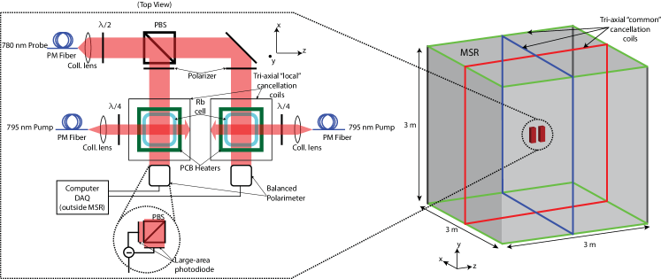
We have developed a diffusion-mode, two-beam SERF magnetometer array configured as a gradiometer for use in fetal magnetocardiography, fMCG Wyllie et al. (2012); Sulai et al. (2013). SERF conditions require working in a near-zero field environment Allred et al. (2002). As a result, we work in a (two-layer mu-metal, 1-layer Aluminum) magnetically shielded room (MSR). The MSR has a residual DC field on the order of 50 nT which we compensate for using active cancellation via a large ($D\approx$ 3 m) set of 3-axis “common” coils wrapped on the perimeter of the MSR and sets of small ($D\approx$ 4 cm) “local” coils wound around each individual magnetometer.

One potential source of magnetic noise is the noise on the currents creating the compensation fields. A 50 nT DC field for example requires a 150 dB$\sqrt{\text{Hz}}$ signal to noise ratio to reach 1 fT/$\sqrt{\text{Hz}}$. We compensate the majority of this DC field with large coils wound near the walls of the room, such that noise associated with these shimming currents is common-mode to a large degree. In practice, we null the field of one of the channels using the large set of coils, and then minimize the residual fields in the other channel ($\leq$ 5 nT) with its set of local coils. This reduces the current noise requirement by 20 dB. In our experiments, the common-mode noise produced by these large sets of coils was measured to be approximately 5 $\text{fT}/\sqrt{\text{Hz}}$ at the location of the magnetometers.

Two channels (shown in Figure 1) are spaced a distance of $L=4\,\rm{cm}$ apart. Each channel comprises a $1\,\rm{cm}^{3}$ Pyrex vapor cell with Rubidium and approximately $200$ Torr of Nitrogen and Neon buffer gas. We heat the cells up to a temperature of $150^{\circ}$ C, elevating the vapor pressure, such that the equilibrium density is $n=10^{14}\,\rm{cm}^{-3}$. The basic idea behind the operation of the SERF magnetometer is that an electron spin polarization $\mathbf{P}$ established by optical pumping interacts with the ambient field, and relaxes at a rate governed primarily by background atom collisions. Rubidium atoms are polarized along $\mathbf{z}$ with circular polarized light resonant with the Rb D1 line at 795 nm. We subsequently detect the projection of $\mathbf{P}$ along the probe direction, $P_{x}$, via off-resonance Faraday rotation using light near the Rb D2 line at 780 nm.

Figure 1: Two SERF magnetometers comprising the gradiometer are placed at the center of a magnetically shielded room. Large (common)coils wrapped around the perimeter of the innermost shield are used to null the total field at one of the magnetometers, as well as to apply calibration signals. Local coils compensate residual gradients. The magnetometers are a distance $L$ = 4 cm apart. A circularly polarized pump beam polarizes a rubidium vapor along the $\hat{z}$ axis. Magnetic fields along $\hat{y}$ (or $\hat{x}$ and $\hat{y}$ in Z-mode) cause rotation of the atomic electron spin polarization which is detected by Faraday rotation of an off-resonance linearly polarized probe beam using a balanced polarimeter.

The spin dynamics of the polarization are described by the Bloch equations and are discussed more fully in Appendix B.

III.1 Operating Modes

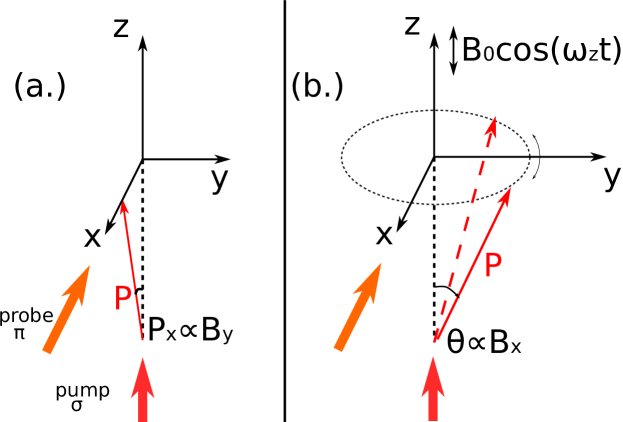
We operate the instrument in either a so called ‘DC mode’ or a parametrically modulated ‘Z-mode.’ In the DC operating mode, the component of the magnetic field perpendicular to the plane of the pump and probe lasers ($B_{y}$) tilts the atomic polarization onto the detection axis Allred et al. (2002); Wyllie IV (2012). This maps $B_{y}(t)$ on to the Faraday rotation signal. See panel (a.) of Figure 2.

Figure 2: Optical pumping along $\mathbf{\hat{z}}$ establishes an electron spin polarization. Off resonance Faraday rotation of the probe light senses the projection of the polarization along the $\mathbf{\hat{x}}$ axis. Panel (a.) shows the DC mode for which $P_{x}(t)\propto B_{y}(t)$. In panel (b.), we show Z-mode, where a modulating field is applied along z, and $P_{x}(t)\propto B_{z}\,\rm{cos}(\omega_{z}t)$

.

In Z-mode, we apply a high frequency modulating magnetic field aligned along the pumping direction ($B_{0}\cos{\omega_{z}t}$, with $\omega_{z}\sim 2\pi\times 1\,\rm{kHz}$) Li, Wakai, and Walker (2006). A field along $\mathbf{\hat{x}}$ torques the polarization $\mathbf{P}$ into the $y-z$ plane at an angle proportional to $B_{x}$. The polarization is modulated at $\omega_{z}$ in the $x-y$ plane as shown in panel (b.) of Figure 2. By demodulating the detected $P_{x}$ signal at $\omega_{z}$, we gain sensitivity to $B_{x}$ at the fundamental frequency (and higher odd harmonics). In addition, we retain sensitivity to $B_{y}$ at DC (and even harmonics of the modulation) Li, Wakai, and Walker (2006). This lock-in technique has the advantage of moving the signal away from DC, to a higher frequency which is free of low frequency laser intensity and polarization noise. Therefore in Z-mode, we can in principle simultaneously detect two components of the magnetic field gradient tensor: $\partial{B_{y}}/\partial{z}$ and $\partial{B_{x}}/\partial{z}$ per the coordinate system shown in Figure 1. For this work, we report measurements where only one component of the tensor was considered at a time.

The DC and Z-mode sensors can be run in open-loop, described above, or in closed-loop, where we use a PID circuit to drive the measured field to zero in the sensitive direction at each sensor position. The compensating signal applied by the servo is then equal to the time varying magnetic field. One of the advantages of running in closed-loop mode is an increased dynamic range. This arises from keeping the average field at the sensor location near zero – thus avoiding saturating the detectors and/or amplifiers. We observe that the closed loop dynamic range is $\sim 100\,\rm{nT}$ compared to $\sim 10\,\rm{nT}$ in the open loop mode. Second, maintaining the field near zero keeps the polarimeter signal balanced. Residual laser intensity fluctuations on the probe can then be suppressed to a higher degree Hobbs (2004). Thirdly, the feedback mode flattens the response of the device through design of the feedback circuit. Operating in closed-loop, we are able to broaden the 3 dB bandwidth of the magnetometers from $\sim 50$ Hz to $\sim 120$ Hz.

III.2 Calibration / Characterization

Due to differences in vapor cell gas composition, temperature, pump and probe laser characteristics etc, the two magnetometers may have different amplitude and phase responses. Their signals cannot be simply subtracted. The full complex response of the two sensors must be properly accounted for. Failure to do so will result in poor common mode rejection due to dephasing errors. Because of this we calibrate the magnetometers against some common calibration signal which we design to ensure adequate coverage of the whole band of interest, as inadequate SNR in the calibration step can limit the achievable CMRR.

Figure 3: Two magnetometer channels comprising a gradiometer were calibrated simultaneously by applying a time dependent field of the form of equation 5 to a common coil shown in (a.). Panel (b.) shows Z-mode open loop response to the applied fields. (c.) shows the closed loop response where the increased bandwidth is clearly evident

.

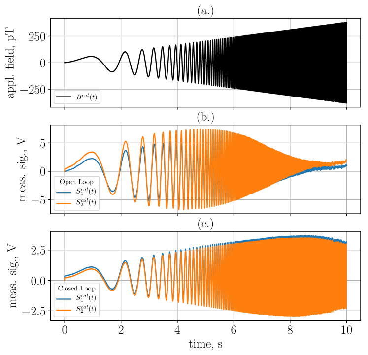
We apply a signal $B^{cal}(t)$ to the large coil and obtain calibration responses from the two channels $S^{cal}_{1}(t)$ and $S^{cal}_{2}(t)$. We choose calibration fields to be of the form

$$B^{cal}(t)=\left(\alpha_{0}+\alpha_{1}t\right)\,\sin(\omega(t)\,t),$$ (5)

where $\omega(t)=\alpha_{2}\exp{\alpha_{3}t}$, with $\alpha_{i}$ positive constants which govern the ‘speed’ of the frequency chirp. This function has an exponentially increasing frequency and a linearly increasing amplitude, which ensures that the SNR for the calibration signal and response does not limit $\xi$ in the DC to 200 Hz frequency range. The applied calibration signal along with the magnetometer responses are shown in Figure 3.

Figure 4: Calibrated response of a single channel of the open-loop magnetometers used in constructing the gradiometer. The total noise is dominated by the magnetic noise in the MSR. The amplitude and phase response is shown on the right.

By taking the Fourier transforms of $B^{cal}(t)$ and $S^{cal}(t)$, we obtain the transfer function of each sensor: $\tilde{M}_{i}(f)=\tilde{S}^{cal}_{i}(f)/\tilde{B}^{cal}(f)$. We interpolate the measured transfer function – obtaining a functional representation of the complex gain which we use to transform subsequent measurements. On acquiring the time series $S_{1}(t)$ and $S_{2}(t)$, we compute a gradiometric signal (in $\rm{fT/cm}$) by calculating

$$\begin{split}G(t)&=(B_{1}(t)-B_{2}(t))/L\\ &=\mathcal{F}^{-1}\left\{\tilde{B}^{cal}(f)\left(\frac{\tilde{S}_{1}(f)}{\tilde{S}^{cal}_{1}(f)}-\frac{\tilde{S}_{2}(f)}{\tilde{S}^{cal}_{2}(f)}\right)\right\}\times\frac{1}{L}\\ &=\mathcal{F}^{-1}\left\{\frac{\tilde{S}_{1}(f)}{\tilde{M}_{1}(f)}-\frac{\tilde{S}_{2}(f)}{\tilde{M}_{2}(f)}\right\}\times\frac{1}{L}\end{split}$$ (6)

where $\mathcal{F}^{-1}$ represents an inverse Fourier transform and $L$ is the gradiometer baseline. We have assumed here that the transfer functions $M_{i}(f)$ are stable on the calibration and measurement time scales. Furthermore, we use the results of the fit to $M_{i}(f)$ to design control servos Deland (2017) for closed loop operation.

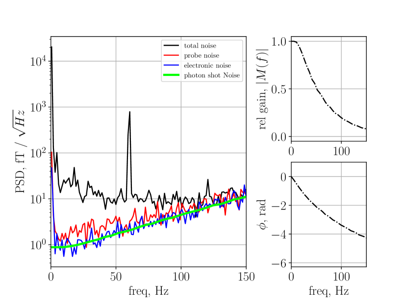
In Figure 4, we plot the complex response of a single magnetometer. The magnetometers’ (DC normalized) relative gain $M(f)=|\tilde{M}(f)|/|\tilde{M}(0)|$ and phase dependence are shown on the two right panels. We also plot the noise spectral density scaled into magnetic field units. The black trace represents the total effective magnetic ambient noise in the room. The probe noise is the noise associated with the intensity and laser polarization fluctuations of the probe laser and has a lower bound given by the photon shot noise.

Figure 5: Complex response function of the different operating modes. The lower plots in each of panels (a.) to (c.) show the gain and phase difference $\Delta M$ and $\Delta\phi$ of two magnetometer channels. These differences are minimized for an optimized configuration.

We measure the probe noise by observing the signal fluctuations with the pump light blocked. Similarly, we measure the electronic noise – the noise due to digitization and EM pickup on the DAQ input lines by blocking both the pump and probe light. In the situation shown in the figure, the magnetic noise dominates all other noise sources. This establishes a margin within which a gradiometer can suppress the uniform component of the magnetic noise. This margin can be amplified by increasing the overall gain of the magnetometer – e.g. by using larger volume cells, or multi-pass cells Sheng et al. (2013); Li, Wakai, and Walker (2006). If the individual magnetometers are limited by technical noise, i.e. probe or electronic noise, then there is no advantage to operating in gradiometric mode. This corresponds to case (0) described in section II.

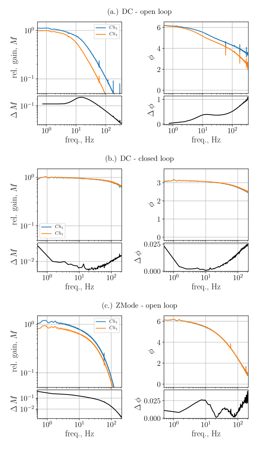
In Figure 5, we show the relative gains of pairs of magnetometers comprising a gradiometer. Panels a - c show DC - open loop implementation, DC - closed loop, and Z-Mode open loop implementations respectively. We plot the difference in response between the two sensor $\Delta M$ and $\Delta\phi$ as the lower plots of each panel. The phase and amplitude response of the two sensor is particularly striking in the open loop operation mode. If not properly accounted for, dephasing errors proportional to $1-\cos{\delta\phi}$, where $\delta\phi$ is the error on $\Delta\phi$, would show up in the difference channel and subsequently in the CMRR. The idea here is that the two channels are vectors in the complex plane, and the dephasing error is the magnitude of the difference vector not accounted for by the calibration.

Panel (b.) shows the measured response of the two gradiometers in DC-mode, closed-loop. Notice the expanded bandwidth, as well as the diminished phase difference. This portends well for achieving high CMRR. Indeed we find that to be the case. The responses are very similar because in closed loop, the shape of the response is dominated by the servo electronics.

Panel (c.) shows the Z-mode open-loop response. One prominent feature of this mode is that the phase response of the two sensors is dominated by the low pass filter associated with the demodulation. Because of the steep phase response we could not, using the same PID loop, apply stable negative feedback over the 0 - 200 Hz band to a Z-mode closed-loop sensor as we did in the the DC-mode closed loop case. We therefore do include Z-mode closed-loop case in our comparisons. Implementing this is on the agenda for future work. We believe however, that the major conclusions of this work stand without it.

Figure 6: Determination of CMRR, $\xi$. White noise is added to the magnetically shielded room via the large coils mounted on the inside surface of the MSR. Panels (a.) and (c.) show the time domain measurements of the individual sensors, as well as their sum and difference. Panels (b.) and (d.) show the power spectral density of the individual as well as of the combined channels. We estimate $\xi$ from the measurements in panel (d). The dotted line is at 2.5 fT/$\sqrt{Hz}\mathrm{cm}$ as a guide for the eye.

Figure 7: Comparison of the CMRR $(\xi)$ for various operating modes. $\xi$ was determined by using equation 1 for measurements made with applied noise as in Figure 6

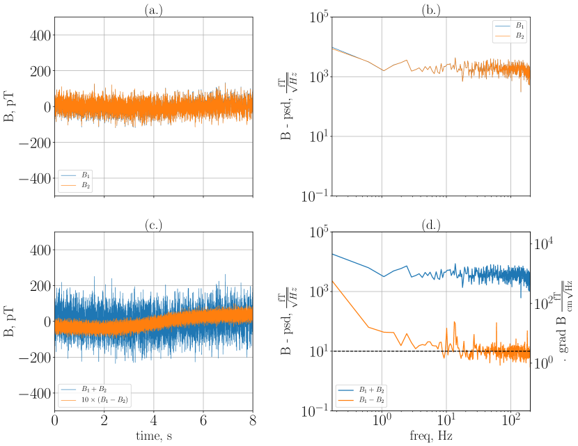
We determined the common-mode rejection ratio $\xi$ of the gradiometer described above by measuring the suppression factor of digitally synthesized white magnetic noise applied to the large coils. It is critical in this step that the amplitude of the applied noise be greater than $\xi$ times the noise floor of the sensors. Otherwise $\xi$ will be underestimated.

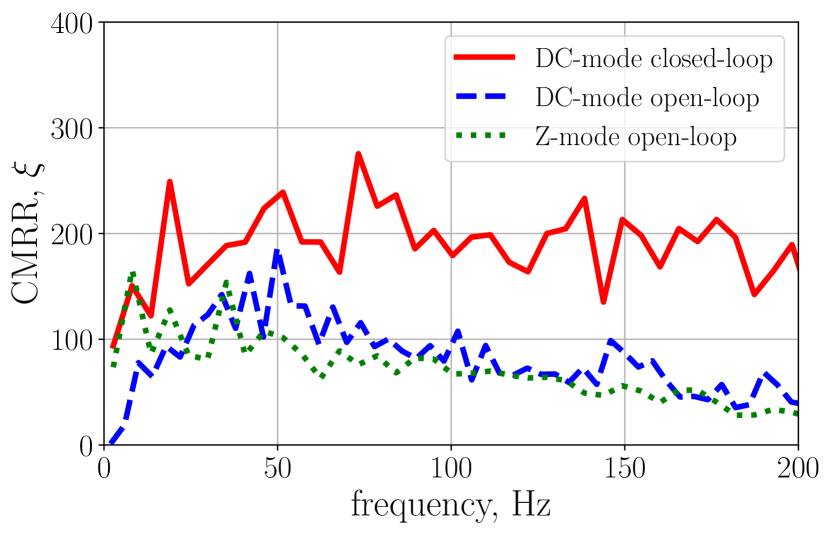
In Figure 6, we show CMRR measurement of the DC - closed loop gradiometer. We observe noise in the difference channel of $<12fT/\sqrt{Hz}$ over a baseline of 4 cm. This corresponds to a magnetic field gradient noise of $<3fT/\mathrm{cm}\sqrt{\mathrm{Hz}}$ In Figure 7, we show a compilation of the measured CMRR for the three operating modes. We found that the DC closed-loop gradiometer had the highest CMRR, with the two open loop cases being comparable. This is summarized in Figure 7.

In summary, we have developed a closed loop first order gradiometer with CMRR $\xi\sim 150$, and gradient noise $<3\,\rm{fT\,cm^{-1}}/\sqrt{\rm{Hz}}$.

Figure 8: The stability of $\xi$ over time was measured in DC-mode with and without active feedback. In the former case, the device was able to maintain an acceptably high level of common-mode noise suppression over a time period comparable to a fMCG measurement. When operating without the feedback, however, the device suffers both in the absolute value of $\xi$ as well as its stability.

IV Gradiometers for fMCG

As noted by Hornberger et al., Hornberger and Collins (2008), “Fetal magnetocardiography (fMCG), the magnetic analog of fetal ECG, is at this time the most effective means of assessing fetal rhythms.” It enables the in-utero diagnoses and monitoring of congenital heart abnormalities Batie et al. (2018). The primary technical challenge of fMCG arises from the relative weakness of the fMCG signal in comparison to background fields – especially the maternal MCG.

Presently, the FDA approved instruments for clinical fMCG applications are SQUID arrays comprising on the order of $\sim 20$ gradiometers, FDA ; Clarke and Braginski (2009). This multiplicity of channels offers an advantage of higher order spatial filtering, or equivalently, the implementation of higher order gradiometers. SQUID based fMCG measurements require magnetically shielded rooms of sufficient size to accommodate the large liquid helium dewars needed for cooling the devices. The required size of the shielded rooms, and the necessary cryogenics, make SQUID gradiometers expensive to set up and operate.

IV.1 MCG signal properties

The magnetic field from a heart is often modeled as that arising from a current dipoleCohen and Hosaka (1976), $B(r_{s})\propto(1/r)^{p}$, with $p\sim 1.8-2.2$ . Consequently, with $g=1+L/r_{s}$, we calculate the the figure of merit for detecting fMCG using equation 3. Given the baseline $L$, and distance from the source $r_{s}$, we choose an optimal sensor for fMCG to be that which maximizes the figure of merit given in equation 3.

Figure 9: Simulated fMCG and MCG wave forms using the ECGSYN program. The power spectral density from the simulation, along as from actual data collected from a recent fMCG data collection run is also shown. Sensors with a bandwidth of $\sim 100\,\mathrm{Hz}$ and sensitivity of a few $\sim 10\mathrm{fT/\sqrt{Hz}}$ will detect the majority of the signal.

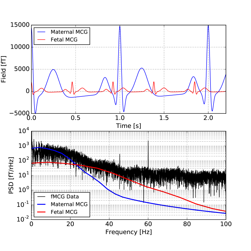
In assessing the interference from the maternal background on the fMCG, we simulated MCG wave forms using the ECGSYN McSharry and Clifford program – scaling the field strengths to the magnitudes typically observed. As shown in Figure 9, the maternal signal is roughly ten times that of the fetus Wyllie IV (2012). This corresponds to an arrangement where the maternal heart signal originates $\sim 60$ cm from the device (compared to the $\sim 5$ cm distance to the fetal heart). We compute and plot in Figure 9 the power spectral density of the two signals, and compare them with the spectral density from a real fMCG measurement obtained using our SERF magnetometers. From this, we posit that for fMCG detection, magnetometers with sensitivity of a few $fT/\sqrt{Hz}$ and bandwidth $\sim 100Hz$ are necessary.

Typically also, fMCG measurements acquired over a ${1\,\rm{to}\,3}$ minute window can be averaged in order to determine relevant MCG parameters such as the time intervals between phases of the MCG waveform. We therefore desire sensors whose calibrations are stable over the course of a measurement interval that is averaged. Finally, the CMRR of the gradiometer will serve to suppress ambient magnetic noise that is uniform. The degree to which it helps suppress the maternal MCG will be described below.

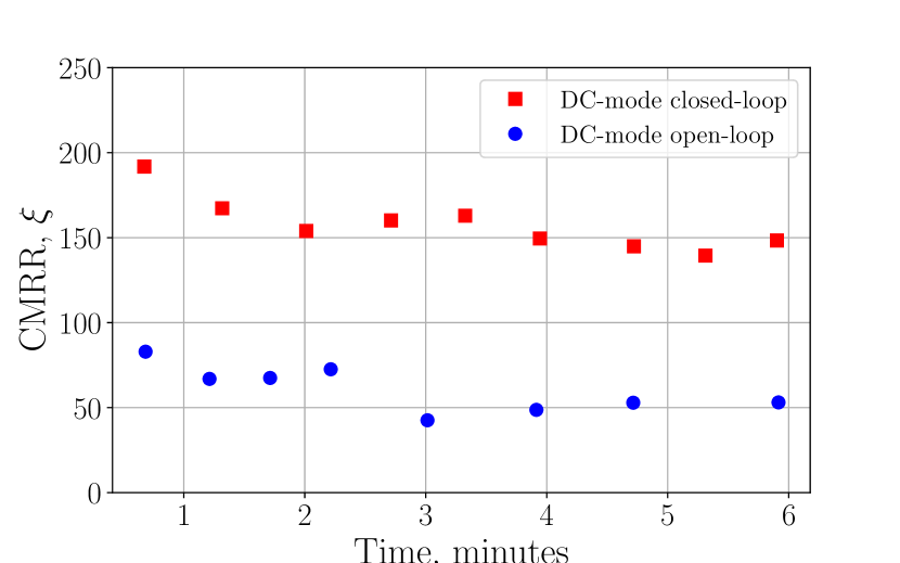
The AM gradiometer we have described above meets the stated sensitivity and bandwidth requirement, along with having $\xi>100$ over the relevant band. It is also stable over the averaging time. We tested this by performing a calibration after which we measured the CMRR over a period of $\sim$ 5 minutes, as shown in Figure 8. The average value of $\xi$ over the band of 1-100 Hz was recorded at various times after calibration in both “open-loop” and “closed-loop” modes. The stability of the CMRR over this interval suggests that the calibration is sufficiently stable for the signals to be averaged. As in previous experiments, we find $\xi$ was superior when operating in closed-loop mode. We did however observe a measurable reduction of $\xi$ with time, and hypothesize that the observed degradation is dominated by residual sensitivity to transverse fields. In our setup, the feedback was only applied along one direction. We suspect that drifts of the field in the other two directions could change the complex response of the two channels. Implementing a scheme where the fields are sensed and compensated in all three directions is one of our priorities for future studies. Operating in closed loop, we find that we can comfortably operate with $\xi>100$.

IV.2 On isolating fetal signal from maternal background

We now consider the question of how effective a gradiometer is in suppressing the maternal background. Modeling the fetal and maternal MCG sources as current dipoles with $B\sim B_{0}/r^{p}$, with $p\sim 2$, we plot in Figure 10 the variation of the fields, their gradients, and their second order gradients with distance from the fetus. We have assumed that the maternal heart is $r_{m}=60$ cm away from the sensor, which is $r_{f}=5$ cm from the fetal heart.

Figure 10: Spatial dependence of the fetal and maternal fields with distance. We assume a $B\propto 1/r^{p}\,(p=2)$ scaling and plot the magnitude of the field along with its first and second order derivatives. This illustrates the advantage of higher order gradiometry in suppressing the maternal signal.

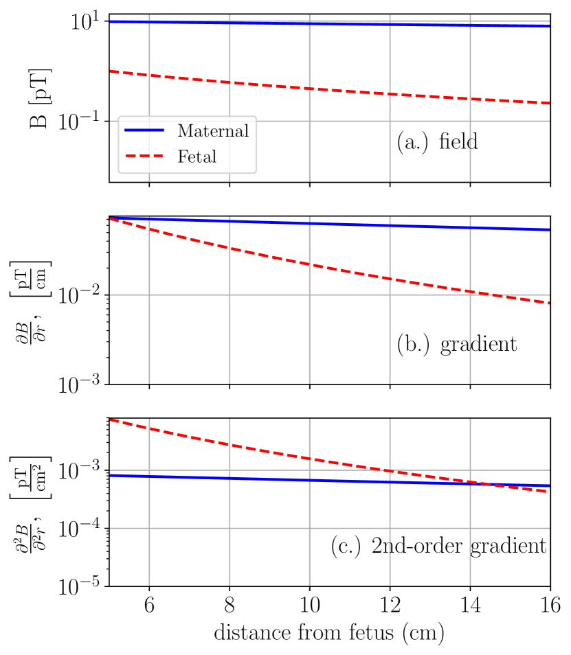
The advantage of using a gradiometer to suppress the maternal contribution to the signal is clear from Figure 10. We see that at $\sim 5\,\rm{cm}$ from the fetus,the maternal field is $\sim 10\times$ larger than the fetal field. The gradients of the field are however comparable in magnitude. A gradient measurement will therefore have less maternal MCG interference. We also see in Figure 10 that we can gain an even greater advantage by detecting the second order gradient. This gain can be obtained if the gradiometers have sufficient sensitivity. For example, in order to detect the fetal gradient at 10 cm with SNR = 1 in 1 second, we surmise (from Figure 10) that we need a sensor with gradient sensitivity $\sim 10\,\rm{fT}\,\rm{cm^{-1}Hz^{-1/2}}$ or better. Likewise, for a second order gradiometer we need a sensitivity of $\sim 10\,\rm{fT}\,\rm{cm^{-2}Hz^{-1/2}}$

Another way to quantify the advantage of the gradiometer is to consider Equation 2. The idea here is that the background to be suppressed is the maternal field $B_{m}\sim B_{0}/r^{p}$. Assuming that the magnetometer has baseline $L$, we then have that ${\delta B_{u}=B_{f}Lp/r_{f}^{p+1}}$, the gradient of the fetal field $\times$ the baseline, and that $\delta B_{c}=B_{m}/r_{m}^{p}$, the average value of the maternal field at the gradiometer. We substitute those values into equation 2 and plot $\mathcal{F}$ for different baselines and CMRRs.

Figure 11: Figure of merit for detecting a fetal field valuated for the case in which the dominant background is the maternal field as shown in figure 9. This calculation illustrates that for our operating condition, $\mathcal{F}$ is limited by the magnitude of the gradient of the maternal field for $\xi>100$

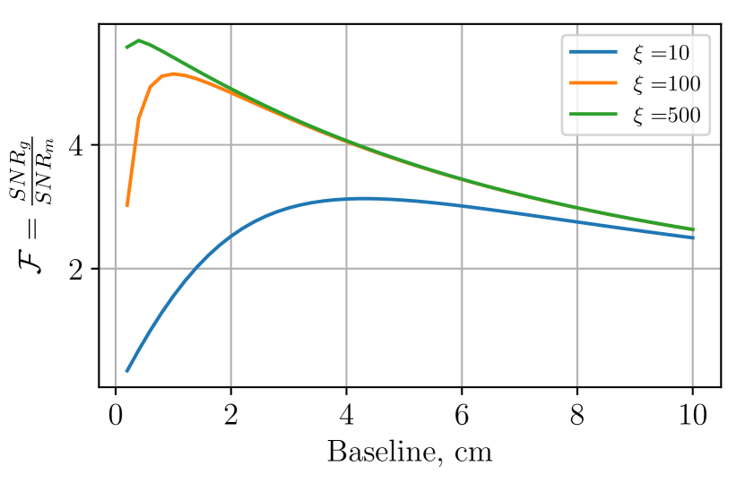
The point to note from Figure 11 is that using a gradiometer for $\xi>100$, the figure of merit is limited by the maternal field gradient, and not the CMRR. With regards to suppressing the maternal signal therefore, there is no advantage to working to increase the CMRR; time is better spent developing a higher order gradiometer. Furthermore, baselines on the order of 1cm are best suited for maternal MCG suppression.

V Comparison to Previous Work

A number of different AM gradiometer implementations have been reported in the literatureAffolderbach et al. (2002); Dang, Maloof, and Romalis (2010); Kominis et al. (2003); Kim et al. (2014); Kamada et al. (2015); Sheng et al. (2013, 2017); Johnson, Schwindt, and Weisend (2010); Xu et al. (2006). Baselines ranging from 0.3 to 10 cm have been attained by either (a) imaging a probe laser going through a single cell onto a segmented photo-detector such as by Kominis et al. Kominis et al. (2003), (b) using spatially separated sensors which requires having multiple probe beams, as in this work, or (c) having a single beam going through multiple cells sequentially as done by Kamada et al. Kamada et al. (2015). Some features of the design choices are that in case (a) the baseline is limited to the size of the cell $\sim 1\,\mathrm{cm}$. One advantage it offers is that atomic responses from the two spatial regions comprising the gradiometer may be very similar as the atoms occupy nearly the same volume. This will enable high CMRR. The designs in cases (b) and (c) allow for larger baselines. For case (c), the subtraction of the signal is effectively performed by Faraday rotation of the probe and not by an electronic circuit or in software. As a result, photon shot noise factors in the total noise budget only once, unlike in case (b) where it factors in twice.

Type	Baseline, L	Mag. Sens	$\xi$	$\mathcal{F}$	bw	Ref
	(cm)	$(\rm{fT/\sqrt{Hz}})$			(Hz)
SQUID	5	5	100	60	$1-150$
SERF	4	10	350	184	$1-150$
SERF	2	10	750	243	$1-150$	Sheng et al. (2017)
SERF	0.8	14	40		$40-400$	Jiang et al. (2019)
NMOR	2.5	80	$>20$			Xu et al. (2006)
SERF	3	9.3	$>6$			Kamada et al. (2015)
SERF	0.5	.16	$<5$			Dang, Maloof, and Romalis (2010)
SERF	$0.3-0.9$	.54	$>13$			Kominis et al. (2003)
SERF	$0.75-12$	4	$>17$			Kim et al. (2014)
SERF	0.5	5	$>3$			Johnson, Schwindt, and Weisend (2010)
SERF	$>2.5$	5	$>6$			Fang et al. (2014)
CPT	1.5	2600	$>800$			Affolderbach et al. (2002)
CsOPM	10	54	$>5$			Koch et al. (2015)
Mx	5	300	1000			Bison et al. (2009)

Table 1: Summary of published results of atomic gradiometers. The figure of merit $\mathcal{F}$ is calculated for $r_{s}=$ 5 cm, and $p=2$–typical values for fMCG Cohen and Hosaka (1976). $\mathcal{F}$ is calculated for an ambient environment sufficiently noisy such that $\left(\delta B_{u}/\delta B_{c}\right)^{2}\ll\xi^{-2}$ and is reported for sensors with well measured $\xi$ and favorable bandwidth for fMCG measurements. The values of $\xi$ for previously-published work should be considered lower bounds.

We compare the different AM gradiometer implementations in Table 1, listing their baselines and the magnetometric sensitivities. We also list CMRRs in situations where it is carefully measured by applying large amplitude noise signal and measuring its suppression. In cases where the CMRR is not well measured, we report the lower limit. Given that the sensitivities and CMRR are functions of frequency, we report their average values over a frequency band of interest. For fMCG, that band is roughly 1 - 100 Hz. Addressing the question of which implementation is best suited for fMCG, we evaluate the figure of merit $\mathcal{F}$ for a source distance characteristic of fMCG in this frequency band.

The evaluated figure of merit $\mathcal{F}$ in Table 1 can be used to assess the suitability of the gradiometer for fMCG in a noisy environment. It does not quantify the degree to which the maternal MCG signal can be suppressed in the fMCG measurement. As discussed in section IV.2, that limitation is due to the non-negligible gradient of the maternal MCG field that is not suppressed by a first order gradiometer.

We note from Table 1 that SERF sensors can achieve comparable and even superior sensitivity and CMRR to SQUIDs. The achieved SERF sensitivity is well established. We have shown here that the CMRR can reliably operate at a few $\times 10^{2}$ over a large frequency range while maintaining this sensitivity.

The chip scale SERF gradiometers described by Sheng et al. Sheng et al. (2017) have the largest figure of merit for an fMCG application of all the sensors we’ve considered. In fact, they report that for the cost of a reduced bandwidth, their closed loop gradiometer can achieve a CMRR of up to 1000 at 10Hz. This is very promising for biomagnetism and low field NMR studiesJiang et al. (2019).

Compared to the chip scale sensors, magnetometers like ours with volumes $\sim\,\rm{cm^{3}}$ have an advantage of a a fundamentally lower spin projection noise level. That sensitivity can be exploited once other sources of technical and uncorrelated magnetic noise are reduced..

As a final point, we recommend that subsequent studies in the development of atomic magnetic gradiometers should report the frequency dependence of their CMRR – measured by adding noise in the frequency range of interest. This specification will enable a more meaningful comparison of techniques and suitability for applications.

VI Conclusion

One key result from this work is that due to differences in temperature, laser intensity distributions, cell wall conditions etc, the individual AM dynamic responses can be different to a degree in which the CMRR can be compromised. As such, we expect that superior gradiometry performance will be obtained if, as described above, a calibration procedure which allows for individual channel differences – factoring their full complex responses – is applied to the sensors comprising the gradiometers. We suspect that even implementations with short baselines where atoms occupy nearly the same volume stand to benefit from this.

We have also in this work introduced a figure of merit $\mathcal{F}$ derived from the gradiometer CMRR, its baseline, and the geometric scaling of the signal and noise background. Knowing this figure of merit will help users judge the optimality of a sensor for a particular application. If the noise background is from a well-known sources (e.g. a current dipole), the noise background scaling can be described analytically. Otherwise, it can be estimated by measuring the gradient noise for a number of baseline values. The optimal baseline is the one that maximizes $\mathcal{F}$

We have demonstrated a gradiometer constructed from two atomic magnetometers with baseline $L=4$ and common-mode rejection ratio $\sim 150$ in the DC to 100 Hz band operating in closed loop. Its performance is comparable with current commercially-available SQUIDs. Future work will include efforts to combine the benefits of parametric-modulation with active feedback to create a superior gradiometer device.

Finally, we note that for the fMCG detection problem, higher order gradiometry is needed. The gradient in the field arising from the maternal MCG which is not suppressed by a first order gradiometer can be comparable to the fMCG. The development of larger count AM gradiometer arrays should therefore be prioritized.

This work was supported by the NIH Eunice Kennedy Shriver National Institute of Child Health & Human Development, No. R01HD057965.

Appendix A Gradiometer Figure of Merit

Consider a configuration as shown in Figure 12. A magnetic field source is located a distance $r_{s}$ from a magnetometer, with a second magnetometer positioned at an additional distance of $L$ along the same axis. The source is assumed to generate a magnetic field with a power law $B(r_{s})\propto(1/r)^{p}$. For example, a point source magnetic dipole in a uniform medium would have a profile with $p=3$. On the other hand, the field from a heart – relevant for MCG – is often modeled as a current dipole Cohen and Hosaka (1976), with $p\sim 1.8-2.2$ .

Figure 12: Configuration of source and magnetometers. The source, a fetal heart, is modeled to be a current dipole $Id\vec{l}$. In the cartoon, the dipole is oriented perpendicular to the axis of the magnetometers, but it should be noted the intra-heart currents that generate the detected fields flow along all three axes.

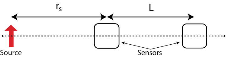
We express the output signal $S_{i}$ of each magnetometer as $S_{i}=M_{i}B(r_{i})$ where $M$ is a response function and $B(r_{i})$ is the field magnitude at a distance $r_{i}$ from the source. The difference signal $S_{G}$ is then given by:

$$S_{G}=S_{1}-S_{2}=M_{1}B_{1}-M_{2}B_{2}.$$ (1)

The signal from a well-balanced (i.e. $M_{1}\approx M_{2}=M$) gradiometer in a magnetic field $B_{i}=B_{0}/r_{i}^{p}$ is

$$S_{G}\approx M(B_{1}-B_{2}) =M\left(\frac{B_{0}}{r_{s}^{p}}-\frac{B_{0}}{\left(r_{s}+L\right)^{p}}\right)$$

$$=\frac{-r_{s}^{p}+\left(r_{s}+L\right)^{p}}{\left(r_{s}+L\right)^{p}}MB_{1}$$

$$=\frac{g^{p}-1}{g^{p}}MB_{1}$$ (2)

where $g=1+L/r_{s}$, and $B_{1}$ is the magnetic field strength at the magnetometer closest to the source.

In practice, the magnetometers can have different amplitude and phase responses to identical magnetic field inputs. The resulting gradiometer consequently will acquire a residual sensitivity to correlated magnetic fields. The undesired residual sensitivity is inversely proportional to the common-mode rejection ratio $\xi$, where

$$\xi =\frac{\frac{1}{2}(S_{1corr}+S_{2corr})}{S_{1corr}-S_{2corr}}$$

$$=\frac{\frac{1}{2}(M_{1}+M_{2})}{M_{1}-M_{2}}.$$ (3)

$S_{icorr}$ is the measured signal from magnetometer $i$ due to an applied correlated field. In SQUID gradiometry Vrba (1996), $\xi$ is limited by the matching pickup coil areas or angular alignment of the two coils. In the case of atomic magnetometers, it is limited by a combination of the noise floor of the magnetometers and the calibration procedure.

In general, a measurement is made in a magnetically noisy environment with total noise $\delta B=\sqrt{(\delta B_{u})^{2}+(\delta B_{c})^{2}}$. $\delta B_{u}$ and $\delta B_{c}$ are the uncorrelated and correlated sources of magnetic noise, respectively. The SNR for the two-channel gradiometer is then

$$SNR_{G} =\frac{\frac{g^{p}-1}{g^{p}}MB_{1}}{\sqrt{(M\delta B_{u1})^{2}+(M\delta B_{u2})^{2}+2\left(M\delta B_{c}\right/\xi)^{2}}}$$

$$=\frac{g^{p}-1}{g^{p}}\frac{B_{1}}{\sqrt{2\left(\delta B_{u}\right)^{2}+2\left(\delta B_{c}/\xi\right)^{2}}}.$$ (4)

where we have made the assumption that $\delta B_{u1}\approx\delta B_{u2}$ for the two magnetometers.

If, instead, the two magnetometers (again, with $M_{1}\approx M_{2}=M$) were not operated as a gradiometer, then the total signal is

$$S_{M} =S_{1}+S_{2}=M\left(B_{1}+B_{2}\right)$$

$$=M\left(\frac{B_{0}}{r_{s}^{p}}+\frac{B_{0}}{\left(r_{s}+L\right)^{p}}\right)$$

$$=\frac{g^{p}+1}{g^{p}}MB_{1}$$ (5)

Thus the signal-to-noise ratio for this two-channel magnetometer is

$$SNR_{M} =\frac{g^{p}+1}{g^{p}}\frac{B_{1}}{\sqrt{2\left(\delta B_{u}\right)^{2}+2\left(\delta B_{c}\right)^{2}}}.$$ (6)

Comparing equations A and 6 illustrates the potential advantage of using a gradiometer, which we define as the gradiometer figure of merit $\mathcal{F}$.

$$\mathcal{F}=\frac{SNR_{G}}{SNR_{M}} =\frac{g^{p}-1}{g^{p}+1}\frac{\sqrt{2\left(\delta B_{u}\right)^{2}+2\left(\delta B_{c}\right)^{2}}}{\sqrt{2\left(\delta B_{u}\right)^{2}+2\left(\delta B_{c}/\xi\right)^{2}}}$$

$$=\frac{g^{p}-1}{g^{p}+1}\frac{\sqrt{\left(\frac{\delta B_{u}}{\delta B_{c}}\right)^{2}+1}}{\sqrt{\left(\frac{\delta B_{u}}{\delta B_{c}}\right)^{2}+\xi^{-2}}}$$ (7)

Gradiometers are only useful if the total noise is dominated by correlated noise between the two channels. Under the assumption that $\delta B_{u}/\delta B_{c}\ll 1$,

$$\mathcal{F}\approx\frac{g^{p}-1}{g^{p}+1}\frac{1}{\sqrt{\left(\frac{\delta B_{u}}{\delta B_{c}}\right)^{2}+\xi^{-2}}}.$$ (8)

This clearly demonstrates the the figure of merit depends on not only the noise ratio of $\delta B_{u}/\delta B_{c}$, but also on how that ratio compares to $\xi$. If $\left(\delta B_{u}/\delta B_{c}\right)^{2}\ll\xi^{-2}$, immediate and potentially substantial benefits to the figure of merit (and therefore gradiometer performance) will be gained through an increase of $\xi$. If, instead, $\left(\delta B_{u}/\delta B_{c}\right)^{2}\gg\xi^{-2}$, further experimental efforts would be best focused elsewhere.

Taking $p=2$ and $L=r_{s}$, for example, we obtain

$$\mathcal{F}\approx\frac{3}{5}\frac{1}{\sqrt{\left(\frac{\delta B_{u}}{\delta B_{c}}\right)^{2}+\xi^{-2}}}.$$ (9)

Appendix B SERF magnetometry

For an ensemble of alkali atoms with total angular momentum F, electronic angular momentum $\mathbf{S}$ and electron spin polarization $\mathbf{P}=2\mathbf{S}$, the SERF regime is where the alkali-alkali spin exchange rate is sufficiently high such that the atoms are described by a spin temperature distribution. We can describe the evolution of angular momentum with the Bloch equation:

$$2\frac{\partial{\left<\mathbf{F}\right>}}{\partial t}=R\left(\mathbf{s}-\left<\mathbf{P}\right>\right)+\mathbf{\Omega}\times\left<\mathbf{P}\right>-\Gamma\left<\mathbf{P}\right>$$ (10)

R is the optical pumping rate, $\mathbf{s}$ the photon angular momentum vector. The magnetic field, $\mathbf{B}=\mathbf{\Omega}/\gamma$ is the given in terms of the Larmor frequency and the gyro-magnetic ratio $\gamma$. $\Gamma$ is the total effective spin relaxation rate. In steady state, equation 10 has solution:

$$\left<\bf{P}\right>=\frac{R}{\Gamma^{\prime}(\Gamma^{\prime 2}+\Omega^{2})}\left(\ \begin{array}[]{c}\Gamma^{\prime}\Omega_{y}+\Omega_{z}\Omega_{x}\\ -\Gamma^{\prime}\Omega_{x}+\Omega_{y}\Omega_{z}\\ -\Gamma^{\prime 2}+\Omega_{z}^{2}\end{array}\right)$$ (11)

where $\Gamma^{\prime}=\Gamma+R$. In our design, we probe the x-component of $\bf{P}$ is probed via off-resonance Faraday rotation.

In near zero field, we have $\mathbf{\Omega}\sim 0$. Consequently

$$P_{x}\sim\frac{R}{\Gamma^{\prime}+\Omega^{2}}\Omega_{y}$$ (12)

In the Z mode case, we apply a modulating field along the pumping direction, such that the total field in equation 10 is now

$${\bf{\Omega}}=\Omega_{x}\hat{x}+\Omega_{y}\hat{y}+(\Omega_{z}+\Omega_{0}\cos(\omega_{z}t))\hat{z}$$

yielding the results:

$$\begin{array}[]{ll}P_{x}(DC)&\approx-\frac{P_{z}}{\Gamma^{\prime}}\Omega_{y}J_{0}(u)^{2}\\ P_{x}(n\omega_{z})&\approx-\frac{P_{z}}{\Gamma^{\prime}}2J_{0}(u)J_{n}(u)\begin{cases}-\Omega_{x}\sin(n\omega_{z}t),&n\text{ odd}\\ -\Omega_{y}\cos(n\omega_{z}t),&n\text{ even}\\ \end{cases}\\ \end{array}$$ (13)

Consequently, we see that the $P_{x}$ signals demodulated at even(odd) harmonics of $\omega_{z}$ lead to sensitivity to $B_{y}$ ($B_{z}$). See Wyllie IV (2012); Deland (2017); Li, Wakai, and Walker (2006) for more detailed description.

References

- Colombo et al. (2016) A. P. Colombo, T. R. Carter, A. Borna, Y.-Y. Jau, C. N. Johnson, A. L. Dagel, and P. D. D. Schwindt, Opt. Express 24, 15403 (2016).
- Sander et al. (2012) T. H. Sander, J. Preusser, R. Mhaskar, J. Kitching, L. Trahms, and S. Knappe, Biomed. Opt. Express 3, 981 (2012).
- Keenan, Blay, and Romans (2011) S. T. Keenan, K. R. Blay, and E. J. Romans, Superconductor Science and Technology 24, 085019 (2011).
- Wiegert and Oeschger (2006) R. Wiegert and J. Oeschger, in OCEANS 2006 (2006) pp. 1–6.
- Jiang et al. (2019) M. Jiang, R. P. Frutos, T. Wu, J. W. Blanchard, X. Peng, and D. Budker, Phys. Rev. Applied 11, 024005 (2019).
- Quartero et al. (2002) H. W. P. Quartero, J. G. Stinstra, E. G. M. Golbach, E. J. Meijboom, and M. J. Peters, Ultrasound in Obstetrics and Gynecology 20, 142 (2002).
- Strasburger, Cheulkar, and Wakai (2008) J. F. Strasburger, B. Cheulkar, and R. T. Wakai, Heart Rhythm 5, 1073 (2008).
- Hämäläinen et al. (1993) M. Hämäläinen, R. Hari, R. J. Ilmoniemi, J. Knuutila, and O. V. Lounasmaa, Rev. Mod. Phys. 65, 413 (1993).
- Clarke and Braginski (2009) J. Clarke and A. I. Braginski, The SQUID Handbook (John Wiley and Sons, Inc, 2009).
- Affolderbach et al. (2002) C. Affolderbach, M. Stahler, S. Knappe, and R. Wynands, Applied Physics B 75, 605 (2002).
- Dang, Maloof, and Romalis (2010) H. B. Dang, A. C. Maloof, and M. V. Romalis, Applied Physics Letters 97, 151110 (2010).
- Kominis et al. (2003) I. K. Kominis, T. W. Kornack, J. C. Allred, and M. V. Romalis, Nature 422, 596 (2003).
- Kim et al. (2014) K. Kim, S. Begus, H. Xia, S.-K. Lee, V. Jazbinsek, Z. Trontelj, and M. V. Romalis, NeuroImage 89, 143 (2014).
- Kamada et al. (2015) K. Kamada, Y. Ito, S. Ichihara, N. Mizutani, and T. Kobayashi, Opt. Express 23, 6976 (2015).
- Sheng et al. (2013) D. Sheng, S. Li, N. Dural, and M. V. Romalis, Phys. Rev. Lett. 110, 160802 (2013).
- Sheng et al. (2017) D. Sheng, A. R. Perry, S. P. Krzyzewski, S. Geller, J. Kitching, and S. Knappe, Applied Physics Letters 110, 031106 (2017).
- Johnson, Schwindt, and Weisend (2010) C. Johnson, P. D. D. Schwindt, and M. Weisend, Applied Physics Letters 97, 243703 (2010).
- Xu et al. (2006) S. Xu, S. M. Rochester, V. V. Yashchuk, M. H. Donaldson, and D. Budker, Review of Scientific Instruments 77, 083106 (2006).
- Wyllie et al. (2012) R. Wyllie, M. Kauer, G. S. Smetana, R. T. Wakai, and T. G. Walker, Physics in Medicine and Biology 57, 2619 (2012).
- Sulai et al. (2013) I. A. Sulai, R. Wyllie, M. Kauer, G. S. Smetana, R. T. Wakai, and T. G. Walker, Opt. Lett. 38, 974 (2013).
- Allred et al. (2002) J. C. Allred, R. N. Lyman, T. W. Kornack, and M. V. Romalis, Phys. Rev. Lett. 89, 130801 (2002).
- Wyllie IV (2012) R. Wyllie IV, The Development of a Multichannel Atomic Magnetometer Array for Fetal Magnetocardiography, Ph.D. thesis, University of Wisconsin-Madison (2012).
- Li, Wakai, and Walker (2006) Z. Li, R. T. Wakai, and T. G. Walker, Applied Physics Letters 89, 134105 (2006).
- Hobbs (2004) P. C. D. Hobbs, Building Electro-Optical Systems: Making it all Work, Vol. I (Wiley-VCH, 2004).
- Deland (2017) Z. J. Deland, Advances in Fetal Magnetocardiography Using SERF atomic magnetometers, Ph.D. thesis, University of Wisconsin-Madison (2017).
- Hornberger and Collins (2008) L. K. Hornberger and K. Collins, Journal of the American College of Cardiology 51, 85 (2008).
- Batie et al. (2018) M. Batie, S. Bitant, J. F. Strasburger, V. Shah, O. Alem, and R. T. Wakai, JACC Clin Electrophysiol. 4, 284 (2018).
- (28) FDA, “005_revised 510(k) summary statement for model 621_624,” https://www.accessdata.fda.gov/cdrh_docs/pdf15/K151135.pdf.
- Cohen and Hosaka (1976) D. Cohen and H. Hosaka, Journal of Electrocardiology 9, 409 (1976).
- (30) P. McSharry and G. Clifford, “Ecgsyn: A realistic ecg waveform generator,” https://www.physionet.org/physiotools/ecgsyn/, accessed 2016.01.07.
- Fang et al. (2014) J. Fang, T. Wang, H. Zhang, Y. Li, and S. Zou, Review of Scientific Instruments 85, 123104 (2014), http://dx.doi.org/10.1063/1.4902567.
- Koch et al. (2015) H.-C. Koch, G. Bison, Z. Grujić, W. Heil, M. Kasprzak, P. Knowles, A. Kraft, A. Pazgalev, A. Schnabel, J. Voigt, and A. Weis, The European Physical Journal D 69, 202 (2015), 10.1140/epjd/e2015-60018-7.
- Bison et al. (2009) G. Bison, N. Castagna, A. Hofer, P. Knowles, J.-L. Schenker, M. Kasprzak, H. Saudan, and A. Weis, Applied Physics Letters 95, 173701 (2009).
- Vrba (1996) J. Vrba, in SQUID Sensors: Fundamentals, Fabrication and Applications, NATO ASI Series, Vol. 329, edited by H. Weinstock (Springer Netherlands, 1996) pp. 117–178.