Hierarchical Event-triggered Learning for Cyclically Excited Systems with Application to Wireless Sensor Networks*

Abstract

Communication load is a limiting factor in many real-time systems. Event-triggered state estimation and event-triggered learning methods reduce network communication by sending information only when it cannot be adequately predicted based on previously transmitted data. This paper proposes an event-triggered learning approach for nonlinear discrete-time systems with cyclic excitation. The method automatically recognizes cyclic patterns in data – even when they change repeatedly – and reduces communication load whenever the current data can be accurately predicted from previous cycles. Nonetheless, a bounded error between original and received signal is guaranteed. The cyclic excitation model, which is used for predictions, is updated hierarchically, i.e., a full model update is only performed if updating a small number of model parameters is not sufficient. A nonparametric statistical test enforces that model updates happen only if the cyclic excitation changed with high probability. The effectiveness of the proposed methods is demonstrated using the application example of wireless real-time pitch angle measurements of a human foot in a feedback-controlled neuroprosthesis. The experimental results show that communication load can be reduced by 70 % while the root-mean-square error between measured and received angle is less than 1^∘.

I Introduction

Many applications require real-time transmission of signals over communication channels with bandwidth limitations. A typical example is given by wireless sensor networks in feedback-controlled systems. The number of agents (i.e., network nodes) and their communication rate is limited by the amount of information the wireless network can transmit in real-time. It is, therefore, desirable to reduce the communication load without compromising the accuracy of the transmitted signals.

Well known approaches are event-based sampling [c1, t1, t2] and event-triggered state estimation (ETSE [t3, t4, t5], sometimes referred to as model-based event-based sampling [c2]): At each sampling instant, the receiving agent independently predicts the state, which is measured by the sender, based on previous estimations and a model. The sender performs the identical prediction and communicates the measured state if and only if the error between prediction and measurement exceeds a predefined threshold. Otherwise, there is no communication and the receiving agent uses the model-based prediction as estimation (cf. Fig. 1).

Figure 1: Event-triggered learning in a two-agents network. If the measured signal (e.g., a human foot angle) can be described by a cyclically excited system model, the model is shared with the receiver and the communication is reduced to those samples that cannot be predicted using the model and previously transmitted data. Inaccuracy of the model (e.g., due to change in walking pattern) is detected and a new model is identified and shared.

Since the prediction accuracy heavily depends on the quality of the utilized model, it was recently proposed to learn and update models in an event-triggered fashion as well [c4]. Occurrence of communication is treated as a random variable, and the model is updated when empirical data does not fit the probability distribution that would result if the model was the truth.

The present paper builds on the idea of [c4] and develops event-triggered learning (ETL) methods for cyclically excited systems. The main contributions are:

• Extension of the concept of ETL to specifically target systems with a locally cyclic excitation. Locally means that cycles close in time are almost identical; however, cycles that are far apart are not necessarily similar. This class of systems is useful for describing both biological and technical processes (e.g., human motion, breath, heartbeat, and production cycles).

• Utilization of a learning trigger tailored to the problem at hand (one-sided Kolmogorov-Smirnov test [ksTest]), which fires with high probability in case of a model change and with low probability otherwise.

• Introduction of the novel idea of a hierarchical model learning strategy, which updates and communicates only a reduced number of model parameters whenever that is sufficient.

• Demonstration of significant communication savings (70 %) using experimental data from cyclic human motion collected with a wearable inertial sensor network. This is the first application of ETL on real-world network data.

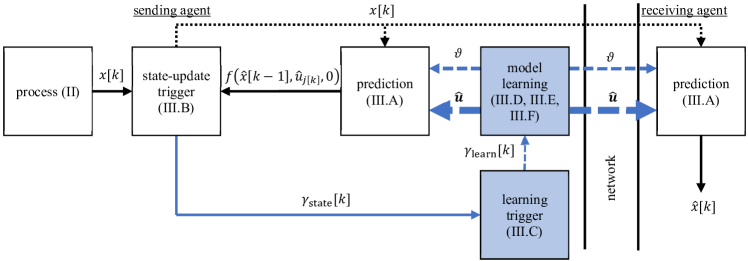
Figure 2: One sending and one receiving agent with the typical event-triggered state estimation architecture in black and event-triggered learning in blue (extended from [c4]). The process provides the measured state $x[k]$ at every sampling instant $k$. At the same time, the state is estimated by the prediction blocks of the sender and the receiver using the previous estimate $\hat{x}\left[k-1\right]$ and a trajectory model of the excitation $\hat{\boldsymbol{u}}$. If the prediction differs significantly from the measured state, then a state update is triggered, and the internal states of both prediction blocks are set to the measured state. Too frequent state updates indicate poor model quality and, therefore, trigger model learning. This can either lead to only an adjustment of certain parameters $\vartheta$ of the current model trajectory or to a completely new excitation trajectory $\hat{\boldsymbol{u}}$. In any case, the new model information is shared between sender and receiver.

The paper continues as follows. After defining the considered problem in Sec. II, the event-triggered learning architecture from [c4] is briefly explained in Sec. III and then extended to cyclically excited systems. Subsequently, the properties of the method are validated experimentally in Sec. LABEL:sec:eval. Finally, Sec. LABEL:sec:conclusions provides conclusions.

II System Representation and Problem Formulation

Consider a discrete-time system with sample index $k\in\mathbb{Z}$ and state $x\left[k\right]\in\mathbb{R}^{n}$, which is measured by the sending agent. The system is assumed to be influenced by a cyclic input $u\left[k\right]\in\mathbb{R}^{m}$ with cycle length $N\in\mathbb{N}^{+}$ such that $u\left[k+N\right]=u[k]$ and by zero-mean noise $\varepsilon\left[k\right]\in\mathbb{R}^{s}$, which is distributed according to a time-invariant probability distribution $\mathcal{P}$. The recursive state update law of the system is characterized by the dynamics $f\colon\mathbb{R}^{n}\times\mathbb{R}^{m}\times\mathbb{R}^{s}\rightarrow\mathbb{R}^{n}$, i.e.,

$$x\left[k\right]=f\left(x\left[k-1\right],u\left[k\right],\varepsilon\left[k\right]\right).$$ (1)

While the dynamics $f$ is assumed to be known, the excitation $u\left[k\right]$ and its cyclicity $N$ are unknown and may change with time. In the following, whenever the term model is used, it refers to an approximation of the cyclic excitation $u\left[k\right]$. The distribution $\mathcal{P}$ of the noise $\varepsilon\left[k\right]$ is known.

This paper considers architectures with one sending and one receiving agent. However, the methods can be directly applied to multi-agent systems and yield the same advantages therein.

The sending and receiving agents have the following capabilities, which will be made precise in the next section:

• the sender can transmit measured data samples to the receiver, i.e., perform state updates;

• sender and receiver can estimate current data samples from previously transmitted data and a model, i.e., perform predictions;

• the sender can estimate excitation trajectories from measured data, i.e., perform model identification;

• the sender can send model parameters to the receiver, i.e., perform model updates.

The main objective is to find a joint strategy for the sender and the receiver such that the amount of communication (state and model updates) is reduced while the error between the actual measurement signal $x\left[k\right]$ and the signal estimate $\hat{x}\left[k\right]\in\mathbb{R}^{n}$ on the receiver side remains small in the sense of a suitable metric $\left\|\cdot,\cdot\right\|\colon\mathbb{R}^{n}\times\mathbb{R}^{n}\rightarrow\mathbb{R}_{0}^{+}$.

III Algorithm Design

The proposed event-triggered learning approach for cyclically excited systems is illustrated in Fig. 2. It can be described by the following building blocks:

• Two identical predictors that estimate the measured state $x[k]$ based on an internal state $\hat{x}[k-1]$ and an estimated excitation trajectory $\hat{\boldsymbol{u}}\in\mathbb{R}^{m\times\hat{N}}$ of one cycle with estimated cycle length $\hat{N}\in\mathbb{N}^{+}$.

• A binary state-update trigger $\gamma_{\text{state}}\left[k\right]\in\left\{0,1\right\}$ that determines when to update the internal state $\hat{x}[k]$ of the predictors with the measurement $x\left[k\right]$ to ensure a bounded error $\left\|x\left[k\right],\hat{x}\left[k\right]\right\|$ of the estimation.

• A model learning block that estimates the excitation trajectory $\hat{\boldsymbol{u}}$ used by the predictors or updates the estimated parameters $\vartheta\in\mathbb{R}^{v}$ (e.g., cycle length or amplitude) of the current trajectory $\hat{\boldsymbol{u}}$.

• A binary learning trigger $\gamma_{\text{learn}}\left[k\right]\in\left\{0,1\right\}$ that determines when to update the internal excitation trajectory model $\hat{\boldsymbol{u}}$ of the predictors. Ideally, learning shall be triggered if and only if the rate of state updates increases due to a false or inaccurate model $\hat{\boldsymbol{u}}$.

III-A Prediction

Let the current model of the cyclic excitation $u\left[k\right]$ be described by the aforementioned matrix $\hat{\boldsymbol{u}}$ such that the current excitation is the $(j[k])^{\text{th}}$ column of $\hat{\boldsymbol{u}}$, i.e., $\hat{u}_{j\left[k\right]}$ is the estimated value of $u\left[k\right]$, where the index $j\left[k\right]$ obeys

$$j\left[k+1\right]=\begin{cases}j\left[k\right]+1&\text{if }\gamma_{\text{learn}}\left[k\right]=0\wedge j\left[k\right]<\hat{N}\\ 1&\text{if }\gamma_{\text{learn}}\left[k\right]=1\vee j\left[k\right]=\hat{N}\end{cases}.$$ (2)

The index $j\left[k\right]$ is increased after every prediction step, unless the end of the estimated excitation trajectory is reached ($j\left[k\right]=\hat{N}$) or learning is triggered ($\gamma_{\text{learn}}\left[k\right]=1$).

The estimate $\hat{x}\left[k\right]$ is determined by

$$\hat{x}\left[k\right]=\begin{cases}f\left(\hat{x}\left[k-1\right],\hat{u}_{j\left[k\right]},0\right)&\text{if }\gamma_{\text{state}}\left[k\right]=0\\ x\left[k\right]&\text{if }\gamma_{\text{state}}\left[k\right]=1\end{cases}.$$ (3)

III-B State-update Trigger

If $d\left[k\right]=\left\|x\left[k\right],f\left(\hat{x}\left[k-1\right],\hat{u}_{j\left[k\right]},0\right)\right\|$ reaches or exceeds the predefined threshold $\delta$, then a state update as defined in Sec. III-A is triggered

$$\gamma_{\text{state}}\left[k\right]=\begin{cases}0&\text{if }d\left[k\right]<\delta\\ 1&\text{if }d\left[k\right]\geq\delta\end{cases}.$$ (4)

Triggers that compare the actual value to a model-based prediction are common in ETSE (cf. [c3, c5, c1, c2, trigger, t3, t4, t5]). Because a state update ($\gamma_{\text{state}}[k]=1$) leads to zero error, (3) and (4) together ensure that $\left\|x\left[k\right],\hat{x}\left[k\right]\right\|$ is bounded by $\delta$.

III-C Robust Learning Trigger

If the model (the estimated excitation trajectory $\hat{\boldsymbol{u}}$) is exact, then state updates occur only due to noise $\varepsilon\left[k\right]$. If the model no longer yields valid predictions of the current data, the time durations between two consecutive state updates will decrease. The learning trigger aims at detecting this decrease and then triggering a model update.

Let the inter-communication time be the discrete time duration (number of samples) between two consecutive state updates and collect these times $\tau_{1},\tau_{2},\ldots,\tau_{i}$ in a buffer, which is emptied whenever model learning is triggered ($\gamma_{\text{learn}}\left[k\right]=1$).

Perform Monte Carlo (MC) simulations of (1), (3), and (4) for the case in which the model $\hat{\boldsymbol{u}}$ is perfect and state updates occur only due to noise. This yields a hypothetical cumulative distribution function $F\colon\mathbb{N}^{+}\rightarrow\left[0,1\right]$ of the inter-communication times. At each sample instant $k$, the aforementioned buffer provides an empirical cumulative distribution function $\hat{F}_{k}\colon\mathbb{N}^{+}\rightarrow\left[0,1\right]$ of the previously observed inter-communication times; i.e., for any value $\tau\in\mathbb{N}^{+}$, $\hat{F}_{k}(\tau)$ is the proportion of observed inter-communication times less than or equal to $\tau$.

The hypothetical and the empirical distribution function of the inter-communication times are compared by the one-sided two-sample Kolmogorov-Smirnov test (KS-test) [ksTest, ksTestTab, ksTestFormula]. Its null hypothesis is that the empirical inter-communication times come from the hypothetical distribution $F(\tau)$. The alternative hypothesis is that they come from a different one. The result of the test is an estimated probability $p\left[k\right]\in\left[0,1\right]$ that the null hypothesis is true. It is compared with a defined significance level $\eta\in\left[0,1\right]$, i.e., the probability that the test rejects the null hypothesis although it is correct (type I error). If the $p\left[k\right]$-value is smaller than $\eta$ for a predefined minimum holding time duration $t_{\min}\in\mathbb{R}_{0}^{+}$, then a model update is triggered

$$\gamma_{\text{learn}}\left[k\right]=\begin{cases}0&\text{if }\exists\;l\in\left[k-t_{\min},k\right]\colon p\left[l\right]\geq\eta\\ 1&\text{if }p\left[l\right]<\eta\;\forall\;l\in\left[k-t_{\min},k\right]\end{cases}.$$ (5)

Note that the null hypothesis is always accepted if no inter-communication times were observed since the last model update. Furthermore, for a large class of systems, the hypothetical distribution $F\left(\tau\right)$ will not depend on $\hat{\boldsymbol{u}}$ and, therefore, can be determined beforehand, i.e., no MC simulations must be performed in real time. Finally, for sufficiently simple systems, the distribution might even be determined analytically, and the one-sided one-sample KS-test can be used.

Utilizing the KS-test to design learning triggers was first proposed in [newPaper]. Density-based learning triggers use richer statistical information and have more advantageous properties than learning triggers that are based on the expected value as proposed in [c4]. In contrast to [newPaper], the current method uses a one-sided trigger condition because model updates are not required if the inter-communication times are larger than expected. The robustification with a minimum holding time $t_{\min}$ prevents model learning due to unmodeled short-term effects. Furthermore, if a change of the process behavior occurs, then learning should not be triggered before the change is completed. For the theoretical properties of the statistical tests to hold, $\tau_{1},\tau_{2},\ldots,\tau_{i}$ are assumed independent and identically distributed (see [c4, newPaper]). While this is not necessarily the case for every system of the form (1), it holds, for example, for the application system considered in Sec. LABEL:sec:eval.

III-D Model Learning – Small Model Update

The model learning block learns a new model trajectory $\hat{\boldsymbol{u}}$ based on the previous measurements $x\left[k\right],x\left[k-1\right],\ldots$ However, transferring the complete trajectory $\hat{\boldsymbol{u}}$ of a cycle from the sending to the receiving agent leads to a significant amount of communication. Therefore, it is assumed that, in some cases, an appropriate new model trajectory $\hat{\boldsymbol{u}}_{+}\in\mathbb{R}^{m\times\hat{N}_{+}}$ with a new cycle length $\hat{N}_{+}$ can be derived from the old one by employing a parametric deformation function $g\colon\mathbb{R}^{m\times\hat{N}}\times\mathbb{R}^{v}\rightarrow\mathbb{R}^{m\times\hat{N}_{+}}$ with a small number of parameters $\vartheta\in\mathbb{R}^{v}$ such that $\hat{\boldsymbol{u}}_{+}=g\left(\hat{\boldsymbol{u}},\vartheta\right)$.

Whenever a learning update is triggered, the learning block determines the parameters $\vartheta$ that lead to the best approximation of the states measured during the last cycle:

$$e(k,\tilde{\vartheta})=\sum_{l=k-\hat{N}_{+}+1}^{k}\|\boldsymbol{x}\left[l\right],\tilde{\boldsymbol{x}}_{\tilde{\vartheta}}\left[l\right]\|^{2},$$ (6)

$$E\left[k\right]=\min_{\tilde{\vartheta}}{e(k,\tilde{\vartheta})},\quad\vartheta=\operatorname*{\arg\!\min}_{\tilde{\vartheta}}{e(k,\tilde{\vartheta})},$$ (7)

where $\tilde{\boldsymbol{x}}_{\tilde{\vartheta}}$ is the state obtained from simulating (1) with excitation $\hat{\boldsymbol{u}}_{+}=g(\hat{\boldsymbol{u}},\tilde{\vartheta})$ and with initial state $x[k-\hat{N}_{+}]$. This value provides an estimate of how good the model would fit after a small update.

Provided the small update is sufficient (see Sec. III-E), the parameters $\vartheta$ are transmitted to the receiver and, subsequently, the receiver determines the new trajectory using the predefined function $g$ and the previous model trajectory $\hat{\boldsymbol{u}}$. For a cyclic process, useful parameters could be cycle length, phase shift, or amplitude, which can be estimated using standard signal processing methods in frequency or time domain to lower the computational costs in comparison to solving the optimization problem (6) explicitly (for an example see Sec. LABEL:sec:eval). Learning of these parameters is always carried out as first step of the block model learning in Fig. 2.

III-E Learning-type Trigger

The small update described above requires much less communication than an update of the full trajectory $\hat{\boldsymbol{u}}$, but might not always lead to sufficiently precise predictions. We define a binary trigger $\gamma_{\text{full}}\left[k\right]\in\left\{0,1\right\}$ that indicates when a small update is not sufficient to achieve a satisfying performance improvement.

If the error $E\left[k\right]$ exceeds a threshold $\alpha\in\mathbb{R}_{0}^{+}$, then a full update is triggered

$$\gamma_{\text{full}}\left[k\right]=\begin{cases}0&\text{if }\gamma_{\text{learn}}\left[k\right]=0\vee E\left[k\right]\leq\alpha\\ 1&\text{if }\gamma_{\text{learn}}\left[k\right]=1\wedge E\left[k\right]>\alpha\end{cases}$$ (8)

and a new full trajectory $\hat{u}$ is identified and transmitted as detailed in Sec. III-F. Otherwise ($\gamma_{\text{full}}\left[k\right]=0$), the sensor sends the parameters $\vartheta$ as small model update and both agents deform the previous excitation trajectory to obtain the new model $\hat{\boldsymbol{u}}=\hat{\boldsymbol{u}}_{+}$. The triggers of both model updates and the state update exhibit a hierarchical dependency: A small model update is only executed if the (communication-wise cheaper) state updates occur too frequently. Likewise, a (communication-wise expensive) full model update is only carried out if a small model update is expected to be insufficient.

III-F Model Learning – Full Model Update

In case of a triggered full update, an appropriate new model $\hat{\boldsymbol{u}}$ cannot be obtained from the previous one by applying the deformation $g$. Therefore, the excitation trajectory for the previously measured cycle is estimated based on the available state measurements. We assume that the dynamics $f$ allow for estimating $u[k]$ from a finite number of state measurements (as is the case in the considered application, see Sec. LABEL:sec:eval).

This trajectory could be transferred directly to the receiving agent via the network and used as a precise model by both prediction blocks for the following state estimations. However, sending all samples of the trajectory would require the network to transfer many values in a short time interval. Therefore, the sender compresses the trajectory at first with polynomial regression and the receiver performs reconstruction to obtain $\hat{\boldsymbol{u}}$. Possible alternatives to polynomial regression for compression are, e.g., wavelet transformation with thresholding of the coefficients [wav], and (sparse) Gaussian process regression [gpr, sparseGpr].

The entire approach described in Sec. III is summarized in Algorithm 1.