Resistivity near a nematic quantum critical point: Impact of acoustic phonons

Abstract

We revisit the issue of the resistivity of a two-dimensional electronic system tuned to a nematic quantum critical point (QCP), focusing on the non-trivial impact of the coupling to the acoustic phonons. Due to the unavoidable linear coupling between the electronic nematic order parameter and the lattice strain fields, long-range nematic interactions mediated by the phonons emerge in the problem. By solving the semi-classical Boltzmann equation in the presence of scattering by impurities and nematic fluctuations, we determine the temperature dependence of the resistivity as the nematic QCP is approached. One of the main effects of the nemato-elastic coupling is to smooth the electronic non-equilibrium distribution function, making it approach the simple cosine angular dependence even when the impurity scattering is not too strong. We find that at temperatures lower than a temperature scale set by the nemato-elastic coupling, the resistivity shows the $T^{2}$ behavior characteristic of a Fermi liquid. This is in contrast to the $T^{4/3}$ low-temperature behavior expected for a lattice-free nematic quantum critical point. More importantly, we show that the effective resistivity exponent $\alpha_{\text{eff}}(T)$ in $\rho(T)-\rho_{0}\sim T^{\alpha_{\text{eff}}(T)}$ displays a pronounced temperature dependence, implying that a nematic QCP cannot generally be characterized by a simple resistivity exponent. We discuss the implications of our results to the interpretation of experimental data, particularly in the nematic superconductor FeSe_1-xS_x.

I Introduction

Recent experiments in several quantum materials have revealed the widespread presence of electronic nematicity, i.e. the lowering of the crystalline point-group symmetry by electronic degrees of freedom Hinkov et al. (2008); Daou et al. (2010); Hashimoto et al. (2012); Fujita et al. (2014); Hosoi et al. (2016); Kuo et al. (2016); Sato et al. (2017); Wang et al. (2018); Coldea and Watson (2018); Böhmer and Kreisel (2018); Ronning et al. (2017). Assessing the impact of these nematic degrees of freedom on the normal-state and superconducting properties of these materials remains an important challenge, particularly near a putative nematic quantum critical point (QCP) Fradkin et al. (2010); Metlitski and Sachdev (2010); Mross et al. (2010); Drukier et al. (2012); Holder and Metzner (2015); Metlitski et al. (2015); Schattner et al. (2016); Lederer et al. (2017); Lee (2018). Experiments provide some evidence that the nematic transition can indeed be tuned to zero temperature by doping or pressure Coldea and Watson (2018); Böhmer and Kreisel (2018); Licciardello et al. (2019). However, progress in elucidating the properties of a nematic quantum critical metal is often hindered by the fact that other types of ordered states are observed concomitantly, such as magnetic order in the pnictides Fernandes et al. (2014), or charge order in the cuprates Keimer et al. (2015). The simultaneous presence of fluctuations associated with multiple ordered phases makes it difficult to disentangle the relevance of the putative nematic QCP to the non-Fermi liquid behavior or to the unconventional superconducting dome often observed in these systems.

However, materials have been recently discovered that seem to display only nematic order, disentangled from other ordered states. This is the case of the chemically substituted iron chalcogenide FeSe_1-xS_x Hosoi et al. (2016): for $x=0$, the system displays a nematic transition at $T_{\mathrm{nem}}\approx 90$ K, whereas for $x=1$ the system is tetragonal. A putative nematic QCP is inferred near the $x\approx 0.18$ concentration, although it is not clear whether the transition is first-order (in which case the QCP would be avoided) or second-order. A nickel-based cousin of the iron pnictides, Ba_1-xSr_xNi₂As₂, and LaFeAsO_1-xF_x also show evidence for a putative nematic QCP without magnetic order Eckberg et al. (2019); Yang et al. (2015), although for the former charge fluctuations may be important. Finally, certain $4f$ intermetallics, such as TmAg₂, undergo a single transition to a nematic phase as temperature is lowered Morin and Rouchy (1993). It has been proposed that shear strain can be used to tune this nematic transition to zero temperature Maharaj et al. (2017), promoting a putative nematic QCP.

These observations motivate a closer theoretical investigation of the metallic nematic QCP and, particularly, of its transport properties, since resistivity is one of the most widely employed probes for non-Fermi liquid behavior. Within the so-called Hertz-Millis approach Hertz (1976); Millis (1993); Löhneysen et al. (2007), in which electronic degrees of freedom are integrated out, the dynamic exponent $z$ characterizing the nematic QCP is the same as that of a ferromagnetic QCP, $z=3$ Rech et al. (2006). This is because Landau damping has the same form in both cases, since the two ordered states have zero wave-vector. A semi-classical Boltzmann-equation approach then predicts that, for a two-dimensional system, the resistivity $\Delta\rho(T)\equiv\rho(T)-\rho_{0}$, where $\rho_{0}$ is the residual resistivity, vanishes as the QCP is approached according to $\Delta\rho(T)\sim T^{4/3}$ Dell’Anna and Metzner (2007); *Metzner-PRL(2009); Löhneysen et al. (2007). Importantly, the presence of impurity scattering to provide a mechanism for momentum relaxation and multiple bands to avoid geometrical cancellation effects are essential Maslov et al. (2011); Pal et al. (2012). Such an exponent, however, has not been observed in recent transport measurements in “optimally doped” FeSe_1-xS_x Licciardello et al. (2019) – in contrast, the resistivity of certain metallic ferromagnets near the QCP seems to be consistent with Hertz-Millis predictions Löhneysen et al. (2007). There are several reasons that could be behind this disagreement, from the possible unsuitability of the Boltzmann-equation approach to describe a system without well-defined quasi-particles to the possible failure of the Hertz-Millis description. Indeed, calculations using the memory matrix formalism have found different temperature dependencies for $\Delta\rho(T)$ Hartnoll et al. (2014); Wang and Berg (2019). Quantum Monte Carlo simulations also provide evidence for non-Hertz-Millis behavior near a nematic QCP Schattner et al. (2016); Lederer et al. (2017).

Although both the ferromagnetic and nematic QCPs are characterized by the same dynamic exponent $z=3$ in the Hertz-Millis approach, a crucial distinction between them is that the nematic order parameter couples linearly to elastic modes of the tetragonal lattice Qi and Xu (2009); Fernandes et al. (2010); Cano et al. (2010); Liang et al. (2013); Karahasanovic and Schmalian (2016); Paul and Garst (2017); Labat and Paul (2017), which are associated with acoustic phonon modes. As a result, the acoustic phonons mediate long-range interactions involving the nematic order parameter Cowley (1976). While these interactions render the classical (i.e., thermal) nematic transition mean-field like, they also restore Fermi-liquid like thermodynamic behavior near the nematic QCP, as shown in Ref. Paul and Garst (2017).

In this paper, we focus on the impact of the coupling to elastic degrees of freedom on the transport properties of a two-dimensional (2D) electronic system close to a nematic QCP. Because this coupling promotes well-defined quasi-particles near the QCP, we employ a Hertz-Millis Boltzmann-equation approach to calculate the temperature-dependence of the resistivity $\Delta\rho(T)$ upon approaching the QCP Ziman (1960); Hlubina and Rice (1995); Rosch (1999); Fernandes et al. (2011). We go beyond the relaxation-time approximation by solving numerically the Boltzmann equation, from which we obtain the non-equilibrium electronic distribution function. Impurity scattering is included as the main source for electronic momentum relaxation. We obtain a momentum-anisotropic distribution function due to the interplay between the $d$-wave nematic form factor and the coupling to the elastic degrees of freedom. The main effect of the latter is to cause the nematic correlation length to diverge only along certain momentum-space directions, as discussed previously in Refs. Karahasanovic and Schmalian (2016); Paul and Garst (2017). At the lowest temperatures, we obtain the standard Fermi-liquid-like behavior $\Delta\rho(T)\sim T^{2}$, which is consistent with the Fermi-liquid behavior previously found in equilibrium thermodynamic properties of the same model Paul and Garst (2017). But our key result is that, upon approaching the nematic QCP, the resistivity cannot be described by a simple power-law $\Delta\rho(T)\sim T^{\alpha}$ over a wide temperature range. Instead, the effective temperature-dependent exponent $\alpha_{\mathrm{eff}}(T)\equiv\partial\ln\left[\Delta\rho(T)\right]/\partial\ln T$ displays a prominent temperature dependence, crossing over from $4/3$ at moderate temperatures to $2$ at very low temperatures. This regime in which $\alpha_{\mathrm{eff}}(T)$ is strongly temperature dependent is particularly sizable for systems with strong nemato-elastic coupling and small Fermi energy, as it is presumably the case of the iron-based superconductors. We also contrast our theoretical results with recent experiments performed in FeSe_1-xS_x Reiss et al. (2019); Licciardello et al. (2019), and discuss the limitations of our approach.

This paper is structured as follows. In Sec. II, we describe the 2D electronic model for the nematic QCP coupled to elastic degrees of freedom. In Sec. III, we give a brief description of the formalism involved in the derivation of the Boltzmann equation and present its numerical solution as a function of temperature as well as other parameters of the model. After that, we describe the low-temperature behavior of the resistivity obtained from the solution of the Boltzmann equation. Lastly, Sec. IV is devoted to the discussion of the results and the presentation of our concluding remarks. The details of some numerical calculations are given in the Appendix.

II Microscopic model

We consider here a two-dimensional tetragonal electronic system coupled to nematic quantum fluctuations and the elastic degrees of freedom of the lattice, similar to that in to Ref. Paul and Garst (2017). The Hamiltonian is given by $\mathcal{H}=\mathcal{H}_{\text{el-nem}}+\mathcal{H}_{\text{nem-latt}}$, where $\mathcal{H}_{\text{el-nem}}$ describes the coupling between the fermions and the $B_{1g}$ nematic order parameter $\phi(\mathbf{q})$, whereas $\mathcal{H}_{\text{nem-latt}}$ denotes, from a renormalization-group point of view, the most relevant coupling of $\phi(\mathbf{q})$ to the local orthorhombic strain $\epsilon(\mathbf{r})=\epsilon_{xx}(\mathbf{r})-\epsilon_{yy}(\mathbf{r})$. Here, strain is defined in the standard way in terms of the displacement vector $\bm{u}$, such that $\epsilon_{ij}=\partial_{i}u_{j}+\partial_{j}u_{i}$ Landau and Lifshitz (1970); Cowley (1976). To keep the analysis as simple as possible, we consider a single circular Fermi surface that has nematic cold spots, with dispersion $\xi_{\mathbf{k}}=\varepsilon_{\mathbf{k}}-\mu$, where $\mu$ is the chemical potential, and write $\mathcal{H}_{\text{el-nem}}$ according to

$$\mathcal{H}_{\text{el-nem}}=\sum\limits_{\mathbf{k},\sigma}\xi_{\mathbf{k}}\psi_{\sigma}^{\dagger}(\mathbf{k})\psi_{\sigma}(\mathbf{k})+\frac{g_{\text{nem}}}{\sqrt{\nu_{0}}}\sum\limits_{\mathbf{k},\mathbf{q},\sigma}h_{\mathbf{k}}\psi_{\sigma}^{\dagger}(\mathbf{k}+\mathbf{q}/2)\psi_{\sigma}(\mathbf{k}-\mathbf{q}/2)\phi(\mathbf{q}),$$ (1)

where $\psi_{\sigma}^{\dagger}(\mathbf{k})$ [$\psi_{\sigma}(\mathbf{k})$] creates (annihilates) electrons with momentum $\mathbf{k}$ and spin projection $\sigma\in\{\uparrow,\downarrow\}$, $g_{\text{nem}}$ is the nematic coupling, and $h_{\mathbf{k}}$ denotes the $d$-wave nematic form factor. We introduced the density of states $\nu_{0}$ for convenience. In the case of a $B_{1g}$ nematic instability, in which the tetragonal symmetry is broken by making the $x$ and $y$ directions inequivalent, $h_{\mathbf{k}}$ is given by:

$$h_{\mathbf{k}}=\cos(k_{x})-\cos(k_{y}),$$ (2)

where the momentum $\mathbf{k}$ is restricted to the vicinity of the Fermi surface. Note that $h_{\mathbf{k}}$ vanishes along the diagonals of the Brillouin zone. Thus, the electronic states at the points where the Fermi surface intercepts these diagonals are effectively uncoupled from the nematic fluctuations. For this reason, they are known as cold spots.

The nematic degrees of freedom are described by the bare propagator:

$$\left(\chi_{\mathrm{nem}}^{0}\right)^{-1}\left(\mathbf{q},i\Omega_{n}\right)=\nu^{-1}_{0}\bigg{(}r_{0}+q^{2}+\frac{\Omega_{n}^{2}}{c^{2}}\bigg{)},$$ (3)

where $c$ is a constant, $\Omega_{n}=2n\pi T$ for $n\in\mathbb{Z}$ is the bosonic Matsubara frequency, and $r_{0}$ is the control parameter proportional to the distance to the bare nematic QCP. Hereafter, all momenta are given in units of the inverse lattice constant, whereas all length scales are given in units of the lattice constant.

As for the Hamiltonian $\mathcal{H}_{\text{nem-latt}}$, it is given by

$$\mathcal{H}_{\text{nem-latt}}=\frac{1}{2}\sum\limits_{\mathbf{q}\neq 0}\bm{u}^{\dagger}(\mathbf{q})\mathcal{\bm{M}}(\mathbf{q})\bm{u}(\mathbf{q})+ig_{\mathrm{latt}}\sum\limits_{\mathbf{q}\neq 0}\mathbf{a}_{\mathbf{q}}\cdot\bm{u}(\mathbf{q})\phi(-\mathbf{q}),$$ (4)

where $\bm{u}(\mathbf{q})$ denotes the Fourier transform of the displacement vector, $\mathbf{a}_{\mathbf{q}}=(q_{x},-q_{y},0)$ is a two-dimensional vector, $g_{\mathrm{latt}}$ represents the nemato-elastic coupling, and $\mathcal{\bm{M}}(\mathbf{q})$ stands for the matrix:

$$\mathcal{\bm{M}}(\mathbf{q})=\begin{pmatrix}C_{11}q_{x}^{2}+C_{66}q_{y}^{2}+C_{44}q_{z}^{2}&(C_{12}+C_{66})q_{x}q_{y}&(C_{13}+C_{44})q_{x}q_{z}\\ (C_{12}+C_{66})q_{x}q_{y}&C_{66}q_{x}^{2}+C_{11}q_{y}^{2}+C_{44}q_{z}^{2}&(C_{13}+C_{44})q_{y}q_{z}\\ (C_{13}+C_{44})q_{x}q_{z}&(C_{13}+C_{44})q_{y}q_{z}&C_{44}(q_{x}^{2}+q_{y}^{2})+C_{33}q_{z}^{2}\end{pmatrix},$$ (5)

with the $C_{ij}$ denoting the elastic constants for a system with tetragonal symmetry Landau and Lifshitz (1970); Cowley (1976).

The effect of the elastic coupling on the nematic degrees of freedom can be evaluated by integrating out the $\bm{u}(\mathbf{q})$ fields. Following the procedure outlined in Ref. Paul and Garst (2017), we first project $\bm{u}(\mathbf{q})$ onto the basis of the polarization vectors of the acoustic phonons $\hat{\bm{e}}_{\mu}(\mathbf{q})$:

$$\bm{u}(\mathbf{q})=\sum_{\mu}U_{\mu}(\mathbf{q})\hat{\bm{e}}_{\mu}(\mathbf{q}).$$ (6)

The polarization vectors are given by the eigenvalue equation $\mathcal{\bm{M}}(\mathbf{q})\hat{\bm{e}}_{\mu}(\mathbf{q})=\varrho\omega_{\mu}^{2}(\mathbf{q})\hat{\bm{e}}_{\mu}(\mathbf{q})$, where $\omega_{\mu}(\mathbf{q})$ are the phonon dispersions and $\varrho$ is the mass density. Next, we use a path integral representation for $\mathcal{H}_{\text{nem-latt}}$ and then integrate out the elastic degrees of freedom. As a result, we obtain the renormalized nematic propagator

$$\chi_{\mathrm{nem}}^{-1}\left(\mathbf{q},i\Omega_{n}\right)=\left(\chi_{\mathrm{nem}}^{0}\right)^{-1}\left(\mathbf{q},i\Omega_{n}\right)-\Pi_{\mathrm{latt}}(\mathbf{q},i\Omega_{n}),$$ (7)

with the polarization bubble:

$$\Pi_{\text{latt}}(\mathbf{q},i\Omega_{n})=\frac{g_{\mathrm{latt}}^{2}}{\varrho}\sum_{\mu}\frac{|\mathbf{a}_{\mathbf{q}}\cdot\hat{\bm{e}}_{\mu}(\mathbf{q})|^{2}}{\omega_{\mu}^{2}(\mathbf{q})+\Omega_{n}^{2}}.$$ (8)

This last expression, when Fourier-transformed back to real space, corresponds to a long-range interaction experienced by the nematic degrees of freedom $\phi(\mathbf{q})$ Paul and Garst (2017). To proceed, since we are mostly interested in layered systems, we hereafter set $q_{z}=0$. By defining the angle $\varphi=\tan^{-1}(q_{y}/q_{x})$ between the two components of $\mathbf{q}$ restricted to the $x$-$y$ plane and the elastic constants combinations $\gamma_{1}=C_{11}+C_{66}$, $\gamma_{2}=C_{11}-C_{66}$, and $\gamma_{3}=C_{12}+C_{66}$, we find that the eigenvalues of $\mathcal{\bm{M}}(\mathbf{q})$ can be written as $\omega_{\mu}(\mathbf{q})=v_{\mu}(\varphi)|\mathbf{q}|$, with anisotropic sound velocities Schütt et al. (2018):

$$v_{\pm}(\varphi) =\frac{1}{\sqrt{2\varrho}}\sqrt{\gamma_{1}\pm\sqrt{\frac{\gamma_{2}^{2}+\gamma_{3}^{2}}{2}+\frac{\gamma_{2}^{2}-\gamma_{3}^{2}}{2}\cos(4\varphi)}},$$ (9)

Accordingly, the normalized eigenvectors of that matrix are given by:

$$\hat{\bm{e}}_{\pm}(\varphi) =\frac{1}{\sqrt{2\Upsilon[\Upsilon\mp\gamma_{2}\cos(2\varphi)]}}\begin{pmatrix}\gamma_{3}\sin(2\varphi)\\ \pm\Upsilon-\gamma_{2}\cos(2\varphi)\\ 0\end{pmatrix},$$ (10)

where $\Upsilon\left(\varphi\right)=\sqrt{\frac{1}{2}(\gamma_{2}^{2}+\gamma_{3}^{2})+\frac{1}{2}(\gamma_{2}^{2}-\gamma_{3}^{2})\cos(4\varphi)}$ is a $C_{4}$-symmetric function.

By inserting Eqs. (9)–(10) into Eq. (8), we can determine straightforwardly the static polarization bubble $\Pi_{\text{latt}}(\mathbf{q},i\Omega_{n}=0)$ and, consequently, the effective mass of the nematic fluctuations defined according to $\nu^{-1}_{0}r\equiv\chi_{\mathrm{nem}}^{-1}(0,0)$. We obtain

$$r(\varphi)=r_{0}-\frac{2g_{\mathrm{latt}}^{2}\nu_{0}}{\gamma_{1}^{2}-\Upsilon^{2}\left(\varphi\right)}\bigg{[}\gamma_{1}+\gamma_{3}-\left(\gamma_{2}+\gamma_{3}\right)\cos^{2}(2\varphi)\bigg{]}.$$ (11)

Note that $r(\varphi)$ is invariant under $\pi/2$ rotations, and has a set of minima for $\varphi_{n}=(2n+1)\pi/4$ with $n\in\mathbb{Z}$. It is convenient to consider the case in which $\frac{C_{11}-C_{12}}{2}=C_{66}$, which corresponds to a lattice that is equally hard with respect to the two types of orthorhombic distortion fluctuations. In this case, one has $\gamma_{2}=\gamma_{3}$ and, consequently, the expression above becomes:

$$r(\varphi)=r_{0}-r_{0,c}+\lambda_{\text{latt}}\cos^{2}(2\varphi),$$ (12)

with $r_{0,c}\equiv\frac{g_{\mathrm{latt}}^{2}\nu_{0}}{C_{66}}$ and $\lambda_{\text{latt}}\equiv\frac{r_{0,c}}{2}\left(1+\frac{C_{12}}{C_{11}}\right)$ being two positive parameters. Thus, the elastic degrees of freedom have two effects: Firstly, they shift the nematic QCP from $r_{0}=0$ to $r_{0}=r_{0,c}>0$ and, secondly, they endow the effective nematic mass with an angular dependence. As a result, the nematic correlation length $\xi_{\mathrm{nem}}\propto r^{-1/2}$ only diverges along the special momentum-space directions $\varphi_{n}=(2n+1)\pi/4$, which coincide with the cold spots positions. This is illustrated in Fig. 1. For this reason, the quantum critical regime becomes directional selective, as discussed in Ref. Paul and Garst (2017). This non-analytic behavior in momentum space can be recast in terms of long-range, dipolar-like interactions in real space involving the nematic order parameter Qi and Xu (2009); Karahasanovic and Schmalian (2016).

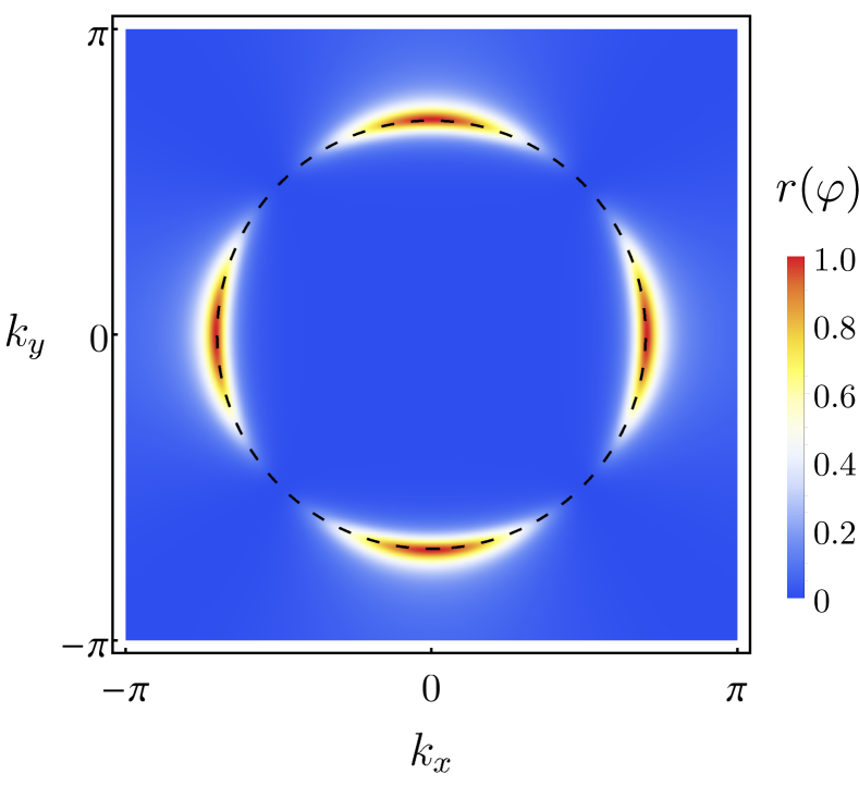
Figure 1: (Color online) Density plot of the effective mass $r(\varphi)$ (in units of $\lambda_{\text{latt}}$) of the critical nematic fluctuations around a circular Fermi surface (dashed black circumference). Notice that $r(\varphi)$ only goes to zero at the cold spots located at the intersection of the Brillouin-zone diagonals with the Fermi surface. In this situation, the quantum critical regime becomes directional-selective.

III Resistivity near the nematic QCP

The consequences of the directional-dependent nematic correlation length, Eq. (11), to the thermodynamic and single-particle electronic properties near the nematic QCP were established in Ref. Paul and Garst (2017). The main result is that, at low enough temperatures, electronic quasi-particles are well-defined, and the system displays a conventional Fermi-liquid behavior. Of course, this temperature scale depends crucially on the nemato-elastic coupling constant $g_{\mathrm{latt}}$. Our goal here is to determine the transport properties near the QCP. While one may be tempted to employ a relaxation-time approximation and replace the transport lifetime by the single-particle lifetime, it is well known that this approximation can be problematic in the case of anisotropic scattering Hlubina and Rice (1995); Rosch (1999, 2000); Fernandes et al. (2011). Furthermore, the relaxation-time approximation makes no reference to momentum relaxation mechanisms, which are particularly important near instabilities with zero wave-vector Maslov et al. (2011).

III.1 Boltzmann equation formalism

We calculate the electrical resistivity by employing a semi-classical Boltzmann-equation approach Ziman (1960); Hlubina and Rice (1995); Rosch (1999); Fernandes et al. (2011). Because the coupling to the elastic degrees of freedom restores well-defined quasi-particles at the QCP, as discussed above, such a semi-classical approach is not unreasonable. We will come back to discuss the shortcomings of this approach in the next section. The main quantity calculated through the Boltzmann equation is the non-equilibrium electronic distribution function $f_{\mathbf{k}}$. In the linearized approximation, which is valid for small departure from equilibrium, it can be expanded as $f_{\mathbf{k}}=f_{\mathbf{k}}^{0}-\Phi_{\mathbf{k}}(\partial f_{\mathbf{k}}^{0}/\partial\varepsilon_{\mathbf{k}})$, where $f_{\mathbf{k}}^{0}\equiv(e^{\beta\xi_{\mathbf{k}}}+1)^{-1}$ is the equilibrium Fermi-Dirac distribution. In this case, the Boltzmann equation is a linear integral equation for $\Phi_{\mathbf{k}}$:

$$-e\mathbf{E}\cdot\mathbf{v}_{\mathbf{k}}\left(\frac{\partial f_{\mathbf{k}}^{0}}{\partial\varepsilon_{\mathbf{k}}}\right)=\frac{1}{T}\sum\limits_{\mathbf{k}^{\prime}}(\Phi_{\mathbf{k}}-\Phi_{\mathbf{k}^{\prime}})f_{\mathbf{k}}^{0}(1-f_{\mathbf{k}^{\prime}}^{0})t_{\mathbf{k},\mathbf{k}^{\prime}},$$ (13)

where $\mathbf{E}$ represents a uniform electric field applied to the electronic quasi-particles with charge $-e$ and $v_{\mathbf{k}}=\nabla_{\mathbf{k}}\varepsilon_{\mathbf{k}}$ is the momentum dependent velocity. The quantity $t_{\mathbf{k},\mathbf{k}^{\prime}}$ is the collision integral; in our problem, we consider that momentum relaxation is provided by collision with impurities. Using the Kadanoff-Baym ansatz Kadanoff and Baym (1962) with the effective self-energy correction in Fig. 2(a) and the Born approximation, the collision integral evaluates to

$$t_{\mathbf{k},\mathbf{k}^{\prime}}= \frac{2g_{\text{imp}}^{2}}{\nu_{0}}\delta(\varepsilon_{\mathbf{k}}-\varepsilon_{\mathbf{k}^{\prime}})+\frac{2g_{\text{nem}}^{2}}{\nu_{0}}h_{(\mathbf{k}+\mathbf{k}^{\prime})/2}^{2}n(\varepsilon_{\mathbf{k}^{\prime}}-\varepsilon_{\mathbf{k}})$$

$$\times\operatorname{Im}[\chi_{\text{nem}}(\mathbf{k}^{\prime}-\mathbf{k},\varepsilon_{\mathbf{k}^{\prime}}-\varepsilon_{\mathbf{k}}+i\eta)],$$ (14)

where $\eta\rightarrow 0^{+}$, $g_{\text{imp}}$ and $g_{\text{nem}}$ [defined previously in Eq. (1)] correspond, respectively, to the impurity and nematic transition rate amplitudes, $n(\omega)\equiv(e^{\beta\omega}-1)^{-1}$ is the Bose-Einstein distribution, and $\chi_{\text{nem}}(\mathbf{q},i\Omega_{n})$ is the nematic susceptibility renormalized by the coupling to both elastic and electronic degrees of freedom. Note that $g_{\mathrm{imp}}$ is proportional to both the impurity scattering potential and the impurity concentration. It is important to note that the nematic fluctuations here are assumed to effectively behave as a bath that is always in equilibrium. This can only be justified if there are additional processes by which the nematic fluctuations equilibrate much faster than the electronic ones. One option is the phonon subsystem, particularly due to the coupling between the nematic order parameter and acoustic phonons, as described by Eq. (1). Morever, if nematic fluctuations arise from separate degrees of freedom (e.g. composite spin order parameters Fernandes et al. (2014)), these fast equilibration processes can take place within the nematic subsystem. However, if the nematic fluctuations arise from a Pomeranchuk-like interaction between low-energy fermions, additional bands are necessary to ensure a finite resistivity and avoid special geometric cancellations Maslov et al. (2011); Pal et al. (2012); Wang and Berg (2019).

Figure 2: Self-energy corrections for (a) the electronic and (b) the nematic degrees of freedom. The electronic and bosonic propagators are denoted here by the solid and dashed lines, respectively. The black dots (“$\bullet$”) correspond to the product of the nematic interaction $g_{\text{nem}}$ with the nematic $d$-wave form factor $h_{\mathbf{k}}$.

Generally, we can write the renormalized nematic susceptibility as:

$$\chi_{\mathrm{nem}}^{-1}\left(\mathbf{q},i\Omega_{n}\right) =\nu^{-1}_{0}\bigg{[}r_{0}+q^{2}+\frac{\Omega_{n}^{2}}{c^{2}}$$

$$-\nu_{0}\Pi_{\mathrm{latt}}(\mathbf{q},i\Omega_{n})-\nu_{0}\Pi_{\mathrm{elec}}(\mathbf{q},i\Omega_{n})\bigg{]},$$ (15)

where $\Pi_{\mathrm{latt}}(\mathbf{q},i\Omega_{n})$ and $\Pi_{\text{elec}}(\mathbf{q},i\Omega_{n})$ are bosonic self-energy corrections due to the coupling to elastic fluctuations and particle-hole excitations [see Fig. 2(b)]. The former was exactly computed in Eq. (8), and its main effect is to replace $r_{0}$ by the renormalized mass $r\left(\varphi\right)$ given by Eq. (12). As for the latter, within a Hertz-Millis approach, its main effect is to change the dynamics of the nematic fluctuations by giving rise to additional frequency-dependent terms:

$$\Pi_{\text{elec}}(\mathbf{q},i\Omega_{n})= -g_{\text{nem}}^{2}\cos^{2}(2\varphi)\frac{|\Omega_{n}|}{v_{F}q}$$

$$-4g_{\text{nem}}^{2}\sin^{2}(2\varphi)\biggl{(}\frac{\Omega_{n}}{v_{F}q}\biggr{)}^{2},$$ (16)

where $v_{F}\equiv|\mathbf{v}_{\mathbf{k}_{F}}|$ is the Fermi velocity. Although the second term yields a sub-leading frequency dependence as compared to the first term, it is the only non-zero term along the directions $\varphi_{n}=(2n+1)\pi/4$ (see also Refs. Hartnoll et al. (2014); Zacharias et al. (2009); Paul and Garst (2017)). These are the same directions along which the renormalized mass $r\left(\varphi\right)$ vanishes, and along which the nematic form factor $h_{\mathbf{k}}$ vanishes, i.e. the cold spots directions.

Within the Boltzmann-equation formalism, the electrical resistivity $\rho(T)$ can be computed by the minimization of the functional Hlubina and Rice (1995); Rosch (1999)

$$\rho[\Phi]=\frac{1}{\nu_{0}e^{2}}\frac{\oint\oint\frac{d\mathbf{k}}{|\mathbf{v}_{\mathbf{k}}|}\frac{d\mathbf{k}^{\prime}}{|\mathbf{v}_{\mathbf{k}^{\prime}}|}\mathcal{F}_{\mathbf{k},\mathbf{k}^{\prime}}(\Phi_{\mathbf{k}}-\Phi_{\mathbf{k}^{\prime}})^{2}}{\Bigl{[}\oint\frac{d\mathbf{k}}{|\mathbf{v}_{\mathbf{k}}|}(\mathbf{v}_{\mathbf{k}}\cdot\hat{\bm{n}})\Phi_{\mathbf{k}}\Bigr{]}^{2}},$$ (17)

where the unitary vector $\hat{\bm{n}}$ points in the direction of the electric field $\mathbf{E}$, the momentum integrals are defined around the Fermi surface, and the function $\mathcal{F}_{\mathbf{k},\mathbf{k}^{\prime}}$ encodes the scattering by impurities and nematic fluctuations. In our case, it is given by

$$\mathcal{F}_{\mathbf{k},\mathbf{k}^{\prime}}= \;g_{\text{imp}}^{2}+g_{\text{nem}}^{2}\frac{h_{(\mathbf{k}+\mathbf{k}^{\prime})/2}^{2}}{T}\int_{-\infty}^{\infty}d\omega\,\omega\,n(\omega)[n(\omega)+1]$$

$$\times\operatorname{Im}[\chi_{\text{nem}}(\mathbf{k}-\mathbf{k}^{\prime},\omega+i\eta)],$$ (18)

with the nematic susceptibility:

$$\chi_{\mathrm{nem}}^{-1}\left(\mathbf{q},i\Omega_{n}\right) =\nu^{-1}_{0}\bigg{[}r_{0}-r_{0,c}+\lambda_{\text{latt}}\cos^{2}(2\varphi)+q^{2}$$

$$+\nu_{0}g_{\text{nem}}^{2}\frac{|\Omega_{n}|}{v_{F}q}\left(\cos^{2}2\varphi+4\sin^{2}2\varphi\,\frac{|\Omega_{n}|}{v_{F}q}\right)\bigg{]}.$$ (19)

Eq. (18) can be evaluated analytically by using the residue theorem and by linearizing the form factor $h_{\mathbf{k}}$ at the Fermi surface. As a result, we find:

$$\mathcal{F}(\mathbf{q})= \;g_{\text{imp}}^{2}+g_{\text{nem}}^{2}\nu_{0}\cos^{2}(2\varphi)\Biggl{[}\left(\frac{B_{\mathbf{q}}-\sqrt{B_{\mathbf{q}}^{2}-4A_{\mathbf{q}}R_{\mathbf{q}}}}{2\pi TA_{\mathbf{q}}\sqrt{B_{\mathbf{q}}^{2}-4A_{\mathbf{q}}R_{\mathbf{q}}}}\right)\psi^{(1)}\left(\frac{B_{\mathbf{q}}-\sqrt{B_{\mathbf{q}}^{2}-4A_{\mathbf{q}}R_{\mathbf{q}}}}{4\pi TA_{\mathbf{q}}}\right)-\left(\frac{B_{\mathbf{q}}+\sqrt{B_{\mathbf{q}}^{2}-4A_{\mathbf{q}}R_{\mathbf{q}}}}{2\pi TA_{\mathbf{q}}\sqrt{B_{\mathbf{q}}^{2}-4A_{\mathbf{q}}R_{\mathbf{q}}}}\right)$$

$$\times\psi^{(1)}\left(\frac{B_{\mathbf{q}}+\sqrt{B_{\mathbf{q}}^{2}-4A_{\mathbf{q}}R_{\mathbf{q}}}}{4\pi TA_{\mathbf{q}}}\right)-\frac{2\pi T}{R_{\mathbf{q}}}\Biggr{]},$$ (20)

where $\mathcal{F}_{\mathbf{k},\mathbf{k}^{\prime}}=\mathcal{F}(\mathbf{k}-\mathbf{k}^{\prime})$, $\psi^{(1)}(z)$ is the trigamma function, $R_{\mathbf{q}}\equiv r_{0}-r_{0,c}+\lambda_{\text{latt}}\cos^{2}(2\varphi)+q^{2}$, $A_{\mathbf{q}}\equiv 4\nu_{0}g_{\text{nem}}^{2}\frac{\sin^{2}(2\varphi)}{(v_{F}q)^{2}}$, and $B_{\mathbf{q}}\equiv\nu_{0}g_{\text{nem}}^{2}\frac{\cos^{2}(2\varphi)}{v_{F}q}$. In order to simplify some of the numerical calculations, we will henceforth approximate $\psi^{(1)}(z)$ by the simpler function

$$\psi^{(1)}(z)\approx\frac{1}{z^{2}}+\frac{18z(z+1)(2z+1)}{(6z^{2}+6z+1)^{2}},$$ (21)

which describes almost exactly the behavior of $\psi^{(1)}(z)$ for $|z|>1$ Mortici (2010). We also note that this approximation does not change the sign of $\mathcal{F}(\mathbf{q})$, which stays positive for all values of the momentum $\mathbf{q}$ and the parameters of the model.

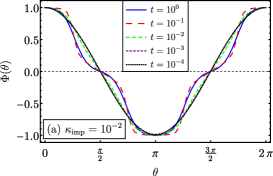
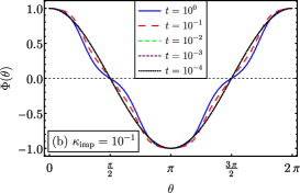
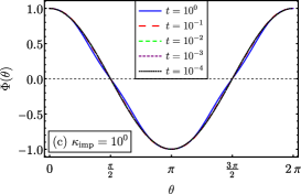
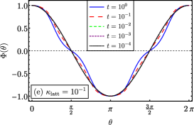
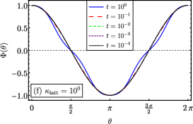
Figure 3: (Color online) Behavior of the normalized quasi-particle distribution $\Phi(\theta)$ obtained by solving Eq. (22) as a function of the reduced temperature $t=T/\varepsilon_{F}$, the dimensionless impurity coupling $\kappa_{\text{imp}}=g^{2}_{\text{imp}}/g^{2}_{\text{nem}}$, and the dimensionless lattice coupling $\kappa_{\text{latt}}=\lambda_{\text{latt}}/(\nu_{0}g^{2}_{\text{nem}})$. In panels (a)–(c), we fix $\kappa_{\text{latt}}=10^{-2}$ and vary $\kappa_{\text{imp}}$, whereas in panels (d)–(f) we set $\kappa_{\text{imp}}=10^{-1}$ and then change the value of $\kappa_{\text{latt}}$. Notice that the effect on the quasi-particle distribution $\Phi(\theta)$ of increasing either the impurity coupling or the lattice coupling is quite similar. In addition, note that $\Phi(\theta)$ approaches asymptotically the cosine function in the low-temperature limit.

The minimization of the functional $\rho[\Phi]$ or, in other words, the demand of the condition $\delta\rho[\Phi]/\delta\Phi=0$, leads to an integral equation for $\Phi_{\mathbf{k}}$ equivalent to the one obtained by the integration of the momentum component perpendicular to the Fermi surface in the Boltzmann equation itself [see Eq. (13)]. For a circular Fermi surface, the equation for the distribution function $\Phi$ in terms of the angle $\theta$ between the momentum $\mathbf{k}$ and the electric field $\mathbf{E}$ becomes a Fredholm equation of the second kind given by

$$\Phi(\theta)=\int_{0}^{2\pi}d\theta^{\prime}\mathcal{K}(\theta,\theta^{\prime})\Phi(\theta^{\prime})+f(\theta),$$ (22)

with:

$$\mathcal{K}(\theta,\theta^{\prime}) \equiv\dfrac{\mathcal{F}(\theta,\theta^{\prime})}{\int_{0}^{2\pi}d\theta^{\prime\prime}\mathcal{F}(\theta,\theta^{\prime\prime})},$$ (23)

$$f(\theta) \equiv\dfrac{\zeta\cos(\theta)}{\int_{0}^{2\pi}d\theta^{\prime\prime}\mathcal{F}(\theta,\theta^{\prime\prime})}.$$ (24)

Here, $\zeta=2\pi^{2}ev_{F}^{2}/k_{F}$ and $\mathcal{F}(\theta,\theta^{\prime})$ is obtained by substituting $2\varphi=\theta+\theta^{\prime}-\pi$ and $q^{2}=4k_{F}^{2}\sin^{2}[(\theta-\theta^{\prime})/2]$ in Eq. (18) for $\mathcal{F}(\mathbf{q})$. It is convenient to separate the terms arising from scattering by impurities and by nematic fluctuations according to $\mathcal{F}(\theta,\theta^{\prime})\equiv g_{\text{imp}}^{2}+g_{\text{nem}}^{2}\mathcal{F}_{\text{nem}}(\theta,\theta^{\prime})$, and express the resistivity as a sum of two terms:

$$\rho(T)=\rho_{\text{imp}}(T)+\rho_{\text{nem}}(T),$$ (25)

where

$$\rho_{\text{imp}}(T)=\frac{\kappa_{\mathrm{imp}}\rho^{0}_{\text{nem}}}{4}\frac{\int_{0}^{2\pi}\int_{0}^{2\pi}d\theta d\theta^{\prime}[\Phi(\theta)-\Phi(\theta^{\prime})]^{2}}{\Bigl{[}\int_{0}^{2\pi}d\theta\cos(\theta)\Phi(\theta)\Bigr{]}^{2}},$$ (26)

$$\rho_{\text{nem}}(T)=\frac{\rho^{0}_{\text{nem}}}{4}\frac{\int_{0}^{2\pi}\int_{0}^{2\pi}d\theta d\theta^{\prime}\mathcal{F}_{\text{nem}}(\theta,\theta^{\prime})[\Phi(\theta)-\Phi(\theta^{\prime})]^{2}}{\Bigl{[}\int_{0}^{2\pi}d\theta\cos(\theta)\Phi(\theta)\Bigr{]}^{2}}.$$ (27)

For convenience, we defined the ratio between the impurity and nematic transition rate amplitudes, $\kappa_{\mathrm{imp}}\equiv g_{\text{imp}}^{2}/g_{\text{nem}}^{2}$, which we refer hereafter as the dimensionless impurity coupling, and the nematic resistivity scale $\rho^{0}_{\text{nem}}\equiv 4g_{\text{nem}}^{2}/(\nu_{0}e^{2}v_{F}^{2})$. Notice that the residual resistivity is given simply by $\rho_{0}\equiv\kappa_{\mathrm{imp}}\rho^{0}_{\mathrm{nem}}$. For later convenience, we also define the ratio between the lattice coupling and the nematic coupling, $\kappa_{\mathrm{latt}}\equiv\lambda_{\text{latt}}/(\nu_{0}g_{\text{nem}}^{2})=\frac{1}{2C_{66}}\left(1+\frac{C_{12}}{C_{11}}\right)\frac{g_{\mathrm{latt}}^{2}}{g_{\text{nem}}^{2}}$, which we refer hereafter as the dimensionless lattice coupling, and the reduced temperature $t\equiv T/\varepsilon_{F}$, where $\varepsilon_{F}=v_{F}k_{F}$ denotes the Fermi energy.

III.2 Solution of the Boltzmann equation

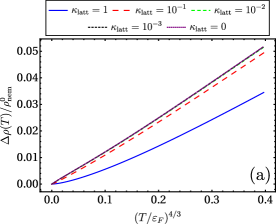
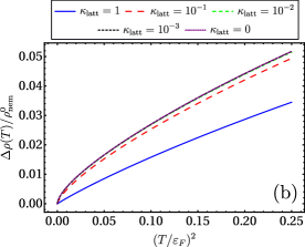
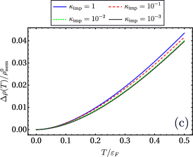
Figure 4: (Color online) (a-b) Behavior of the resistivity $\Delta\rho(T)=\rho(T)-\rho_{0}$ as a function of the temperature $T$ and the dimensionless lattice coupling $\kappa_{\text{latt}}$. We fix here the dimensionless impurity coupling to $\kappa_{\text{imp}}=10^{-1}$. In the absence of $\kappa_{\text{latt}}$, the low-temperature behavior of the resistivity is characterized by $\Delta\rho(T)\sim T^{4/3}$ [panel (a)], although when $\kappa_{\text{latt}}$ is $\mathcal{O}(1)$, namely when the lattice coupling $g_{\text{latt}}$ is comparable to the nematic interaction $g_{\text{nem}}$, the resistivity is given by $\Delta\rho(T)\sim T^{2}$ [panel (b)]. (c) This behavior is rather insensitive to changes in the impurity coupling $\kappa_{\text{imp}}$, particularly at low temperatures. In this particular case, we fix $\kappa_{\text{latt}}=0.5$.

We first solve analytically the Boltzmann equation in the low-temperature regime near the QCP, which corresponds to setting $r_{0}=r_{0,c}$. At low enough temperatures, inelastic scattering by nematic fluctuations is always subleading with respect to the elastic scattering by impurities. Of course, this temperature scale depends on the dimensionless lattice coupling $\kappa_{\mathrm{latt}}$, which we consider to be finite. In this regime, the out-of-equilibrium distribution function can be well approximated by the solution of the Boltzmann equation in the presence of impurity scattering only, which gives the standard expression $\Phi(\theta)=\cos(\theta)$ for the normalized distribution function Ziman (1960).

We first consider the case in which the coupling to the lattice vanishes, $\kappa_{\mathrm{latt}}=0$. By employing Eq. (21), we are able to approximate $\mathcal{F}(\mathbf{q})$ in the low-temperature limit by the expression

$$\mathcal{F}(\mathbf{q})\approx g^{2}_{\text{imp}}+g^{2}_{\text{nem}}\nu_{0}\cos^{2}(2\varphi)\frac{4\pi^{2}B_{\mathbf{q}}T^{2}}{3(R_{\mathbf{q}}+2\pi B_{\mathbf{q}}T)^{2}},$$ (28)

where $R_{\mathbf{q}}=r_{0}+q^{2}$. In this situation, the electrical resistivity [see Eqs. (25)–(27)] evaluates to

$$\rho(T)=\rho^{0}_{\text{nem}}\bigg{[}\kappa_{\text{imp}}+\frac{2^{1/3}\Gamma\left(-\frac{4}{3}\right)\Gamma\left(\frac{11}{6}\right)\nu^{1/3}_{0}g^{2/3}_{\text{nem}}}{27\pi^{7/6}k^{2/3}_{F}}\bigg{(}\frac{T}{\varepsilon_{F}}\bigg{)}^{4/3}\bigg{]},$$ (29)

with $\Gamma(z)$ being the Gamma function. Therefore, we reproduce within the Boltzmann-equation formalism the expected $T^{4/3}$ scaling behavior of the resistivity for a dirty 2D electronic system close to a nematic QCP.

We now move to the case where the coupling to the lattice $\kappa_{\text{latt}}$ is finite. By making use once again of Eq. (21) and then considering the temperature range $T\ll\kappa^{3/2}_{\text{latt}}\varepsilon_{F}$, one finds

$$\mathcal{F}(\mathbf{q})\approx g^{2}_{\text{imp}}+g^{2}_{\text{nem}}\nu_{0}\cos^{2}(2\varphi)\frac{4\pi^{2}B_{\mathbf{q}}T^{2}}{3R^{2}_{\mathbf{q}}}.$$ (30)

As a result, for the range of nemato-elastic interactions defined by $0<\kappa_{\text{latt}}\lesssim k^{2}_{F}/(\nu_{0}g^{2}_{\text{nem}})$, the electrical resistivity at the nematic QCP becomes

$$\rho(T)=\rho^{0}_{\text{nem}}\bigg{[}\kappa_{\text{imp}}+\frac{\mathcal{C}_{0}}{\kappa_{\text{latt}}}\bigg{(}\frac{T}{\varepsilon_{F}}\bigg{)}^{2}\bigg{]},$$ (31)

where $\mathcal{C}_{0}\approx 0.17$ is a numerical constant. Consequently, the resistivity in this particular case describes Fermi-liquid-like behavior, which agrees with the results in Ref. Paul and Garst (2017) based on the calculations of thermodynamics and single-particle properties.

Our asymptotic analysis for the low-temperature behavior of the resistivity suggests that a crossover from $\Delta\rho(T)\sim T^{4/3}$ at moderate temperatures to $\Delta\rho(T)\sim T^{2}$ at low temperatures can be expected, with the crossover temperature scale being determined by the dimensionless lattice coupling $\kappa_{\mathrm{latt}}$. To verify this expectation, we numerically solve the integral equation (22) to find the non-equilibrium distribution function $\Phi\left(\theta\right)$ and then compute the resistivity in Eqs. (26) and (27). To make the numerical calculations convergent, we consider that at the QCP the effective nematic mass vanishes linearly with temperature, i.e. $r_{0}=r_{0,c}+a(T/\varepsilon_{F})$. Such a linear $T$ dependence is characteristic of a mean-field behavior, which is theoretically expected to the be case for the nematic transition due to the coupling to the lattice (see Ref. Karahasanovic and Schmalian (2016)); this is also the experimentally observed behavior Kuo et al. (2016); Böhmer and Kreisel (2018). Here, we set the dimensionless constant $a$ to be $a=1$. As explained in more details in the Appendix, the low-temperature behavior of $\Delta\rho(T)$ is independent of the value of $a$.

In Fig. 3, we show the numerical solution for the non-equilibrium distribution function $\Phi(\theta)$ by varying the reduced temperature $T/\varepsilon_{F}$, the impurity coupling $\kappa_{\mathrm{imp}}$, and the lattice coupling $\kappa_{\mathrm{latt}}$. It is clear that, at low enough temperatures, the distribution function always approaches the $\cos(\theta)$ function, characteristic of the impurity-scattering only problem. As discussed above, this is a consequence of the fact that, at low enough temperatures, inelastic scattering is subleading compared to elastic scattering. As a result, by comparing panels (a)-(c), which have the same $\kappa_{\mathrm{latt}}=10^{-2}$ parameter, it is clear that the temperature scale below which the distribution function approaches $\cos(\theta)$ increases as $\kappa_{\mathrm{imp}}$ increases. Above this temperature scale, the main deviations from the $\cos(\theta)$ distribution are located at the angles $\theta_{n}=(2n+1)\pi/4$, which correspond to the cold spots of the Fermi surface. Although this may seem contradictory at first sight, since the nematic form factor vanishes for quasi-particle scattering at the cold spots, one can understand this behavior as arising from the simple fact that we have to average over all processes within the Fermi surface to find the quasi-particle distribution. Consequently, this also depends on the Fermi-surface regions where the nematic form-factor contribution is finite. Furthermore, we also notice that the zeros of the quasi-particle distribution $\Phi(\theta)$ occur at the same points where the function $\cos(\theta)$ goes to zero. In fact, at these points the Boltzmann equation becomes a homogeneous integral equation [see Eq. (22)], which has only a trivial solution due to the dependence of $\mathcal{K}(\theta,\theta^{\prime})$ on the impurity coupling $\kappa_{\text{imp}}$.

In panels (d)–(f), we fix $\kappa_{\mathrm{imp}}=10^{-1}$ and vary the dimensionless lattice coupling $\kappa_{\mathrm{latt}}$. It is interesting to note that the nemato-elastic coupling plays a similar role as the disorder coupling, in the sense that it also favors a distribution function that is similar to the $\cos(\theta)$ distribution. The reason is because the coupling to the lattice makes the nematic mass finite everywhere except at the cold spots, thus removing much of the strongly anisotropic behavior associated with the nematic QCP.

Having determined $\Phi(\theta)$ numerically, we plot in Fig. 4 the temperature-dependence of the resistivity $\Delta\rho(T)\equiv\rho(T)-\rho_{0}$. In panels (a)-(b), we fix the impurity coupling to $\kappa_{\mathrm{imp}}=10^{-1}$ and vary the lattice coupling $\kappa_{\mathrm{latt}}$. As shown in panel (a), when the nematic degrees of freedom are uncoupled from the lattice, $\kappa_{\mathrm{latt}}=0$, we find the expected $\Delta\rho(T)\sim T^{4/3}$ behavior of a nematic QCP. Upon increasing $\kappa_{\mathrm{latt}}$, we start noting deviations from this power law. In particular, when $\kappa_{\mathrm{latt}}\sim 1$, there is a wide range of temperatures in which $\Delta\rho(T)\sim T^{2}$, as illustrated in panel (b). However, for intermediate values of $\kappa_{\mathrm{latt}}$, it is clear that the temperature dependence of the resistivity cannot be described by a single power law. This is reminiscent of the effect of impurity scattering on the resistivity near an antiferromagnetic QCP, which makes the temperature dependence of $\Delta\rho(T)$ not display a simple power-law behavior Rosch (1999, 2000). In our case, however, impurity scattering has little effect on the temperature dependence of $\Delta\rho(T)$, as shown in panel (c). The main effect comes from the coupling to the lattice $\kappa_{\mathrm{latt}}$, which endows the nematic susceptibility with an anisotropic correlation length.

To better illustrate the behavior of $\Delta\rho(T)$ near the nematic QCP coupled to the lattice, we plot in Fig. 5 the effective temperature-dependent exponent $\alpha_{\mathrm{eff}}(T)\equiv\partial\ln\left[\Delta\rho(T)\right]/\partial\ln T$ for different values of the lattice coupling $\kappa_{\mathrm{latt}}$. It is clear that, for $\kappa_{\mathrm{latt}}<1$, the exponent varies between the approximate range $4/3\lesssim\alpha_{\mathrm{eff}}(T)\lesssim 2$, as anticipated from our analytical results. Note that the $T^{2}$ behavior may be achieved only at extremely low temperatures, depending on the value of $\kappa_{\mathrm{latt}}$. Similarly, the $T^{4/3}$ behavior may be essentially inaccessible if $\kappa_{\mathrm{latt}}$ is not small enough.

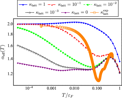
Figure 5: (Color online) Temperature-dependent effective exponent $\alpha_{\mathrm{eff}}(T)$ of the electrical resistivity $\Delta\rho(T)\sim T^{\alpha_{\mathrm{eff}}(T)}$ for different values of the dimensionless lattice coupling $\kappa_{\text{latt}}$ and fixed dimensionless impurity coupling $\kappa_{\text{imp}}=10^{-1}$. At very low temperatures and at a finite value of $\kappa_{\text{latt}}$, $\alpha_{\mathrm{eff}}(T)$ will eventually saturate at $\alpha_{\mathrm{eff}}=2$, which marks the emergence of Fermi-liquid regime for the system. The bigger empty circles, indicated by $\kappa^{\text{exp}}_{\text{latt}}$, are the experimental data reported in Ref. Bristow et al. (2019) for the resistivity exponent $\alpha_{\mathrm{eff}}(T)$ of “optimally” doped FeSe_1-xS_x with $x=0.18$, which harbors a putative nematic QCP. Here, we used the value $\varepsilon_{F}=250$ K for the Fermi energy of this material.

IV Concluding remarks

In summary, we evaluated the impact of the coupling to the elastic degrees of freedom on the electrical resistivity near a two-dimensional metallic nematic QCP. Our main result is that the temperature-dependent resistivity $\Delta\rho(T)=\rho(T)-\rho_{0}$ cannot generally be described by a simple power law. This is a consequence of the fact that the elastic coupling favors, at low enough temperatures, a Fermi-liquid like behavior, characterized by $\Delta\rho(T)\sim T^{2}$. In contrast, quantum critical nematic fluctuations, which are cutoff by the lattice coupling, favor a $\Delta\rho(T)\sim T^{4/3}$ behavior. As a consequence of these opposing tendencies, the effective exponent $\Delta\rho(T)\sim T^{\alpha_{\mathrm{eff}(T)}}$ shows a pronounced temperature dependence, as illustrated in Fig. 5, roughly crossing over between $4/3$ and $2$.

The lattice is always present in real systems, and its effects on the nematic degrees of freedom are profound even in the qualitative level, as manifested in the directional-dependence of the nematic correlation length. Thus, a full understanding of experimental data requires elucidating how the elastic degrees of freedom affect the transport properties near the nematic QCP. Before discussing comparisons with experimental results, it is important to further discuss the limitations of our approach. The main reason to consider a Boltzmann-equation approach is because quasi-particles are well-defined near the nematic QCP due to the coupling to the elastic degrees of freedom, as previously shown in Ref. Paul and Garst (2017). Of course, as the coupling to the lattice becomes smaller, this approximation becomes more questionable. Furthermore, even within this approximation, it is not obvious that the Hertz-Millis approach employed here to account for the dynamics of the nematic fluctuations will hold. It would be interesting, in this regard, to go beyond the Boltzmann equation approach and consider a different technique, such as the memory matrix formalism Forster (1975). Previous applications of this approach to the transport properties of the nematic QCP revealed important deviations from the expectations of the Boltzmann-equation approach under certain conditions Hartnoll et al. (2014); Wang and Berg (2019). In particular, the recent work Wang and Berg (2019) found an interesting broad temperature range in which the resistivity displays a linear-in-$T$ behavior, which is absent in the Boltzmann formalism. However, the impact of the lattice degrees of freedom was not considered in those investigations. Similarly, sign-problem-free Quantum Monte Carlo simulations Schattner et al. (2016); Lederer et al. (2017) of the coupled nemato-elastic QCP would be desirable.

The most transparent experimental evidence of an isolated putative nematic QCP is on the phase diagram of FeSe_1-xS_x Hosoi et al. (2016). While the very large values of the nematic susceptibility and its temperature dependence suggest a second-order transition, the sudden drop of the nematic transition temperature for a small change of doping concentration $x$ is typical of first-order transitions. The temperature dependence of the resistivity near this possible nematic QCP has been experimentally studied. Ref. Licciardello et al. (2019) finds a wide temperature regime near the nematic QCP at the concentration $x_{c}$ where the resistivity displays a nearly linear behavior, which is not captured by our model. This could be suggestive of additional excitations at play or non-Hertz-Millis behavior. On the other hand, Ref. Bristow et al. (2019) reported a temperature dependence of $\alpha_{\mathrm{eff}}$ that is qualitatively consistent with our findings, increasing from close to $3/2$ at higher temperatures to close to $2$ at lower temperatures. The data points are also shown in Fig. 5, for comparison. A similar temperature dependence of $\alpha_{\mathrm{eff}}$ was observed in Ref. Reiss et al. (2019) when the nematic QCP was tuned by pressure in an “underdoped” composition of FeSe_1-xS_x. Of course, while our model is certainly too simplified to capture the complex band structure of FeSe_1-xS_x, the overall trend in $\alpha_{\mathrm{eff}}$ is what one would expect from our analysis. Overall, our work unveils the crucial role played by the lattice on the transport properties near a nematic QCP.

Appendix: Details of the numerical solution of the Boltzmann equation

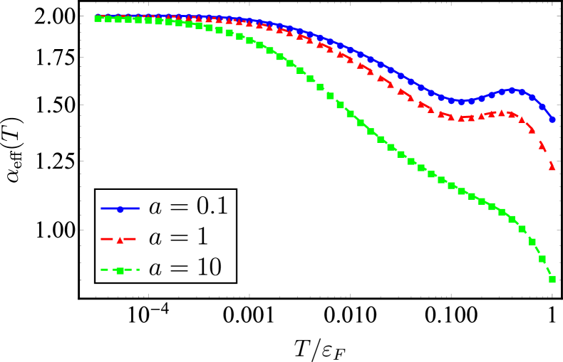
Figure A1: (Color online) Dependence of the effective exponent $\alpha_{\mathrm{eff}}(T)$ of the electrical resistivity $\Delta\rho(T)\sim T^{\alpha_{\mathrm{eff}}(T)}$ on the nematic mass $r_{0}=r_{0,c}+\delta(T)$ for $\delta(T)=a(T/\varepsilon_{F})$. We fix here the impurity scattering and the elastic coupling according to $\kappa_{\text{imp}}=10^{-1}$ and $\kappa_{\text{latt}}=10^{-1}$, respectively. In the low-temperature regime, one can notice that the behavior of $\alpha_{\mathrm{eff}}(T)$ is not altered by the value of the constant $a$.

As discussed in the main text, to reach numerical convergence we included the temperature dependence of the effective nematic mass at the nematic QCP, i.e., we set $r_{0}=r_{0,c}+\delta(T)$. This is a reasonable assumption, since the correlation length only diverges at the QCP. Since a full self-consistent calculation of $\delta(T)$ is beyond the scope of our Boltzmann-equation calculations, here we employ a phenomenological approach. Motivated by the experimental observations Kuo et al. (2016); Böhmer and Meingast (2016) that the nematic susceptibility in iron-based superconductors displays an approximate Curie-Weiss behavior, $\chi_{\mathrm{nem}}\propto(T-T_{\mathrm{nem}})^{-1}$, we set near the QCP (where $T_{\mathrm{nem}}=0$) $\delta(T)=a(T/\varepsilon_{F})$, where $a$ is a dimensionless constant. As shown in Fig. A1, and already anticipated by the analytic results in Eqs. (29) and (31), the value of $a$ does not change the low-temperature behavior of $\Delta\rho(T)$. It does affect how the effective exponent $\alpha_{\mathrm{eff}}(T)$ behaves at high temperatures, which is not unexpected, since at high temperatures the resistivity exponent is not universal.

References

- Hinkov et al. (2008) V. Hinkov, D. Haug, B. Fauqué, P. Bourges, Y. Sidis, A. Ivanov, C. Bernhard, C. T. Lin, and B. Keimer, Electronic Liquid Crystal State in the High-Temperature Superconductor YBa2Cu3O6.45, Science 319, 597 (2008).
- Daou et al. (2010) R. Daou, J. Chang, D. LeBoeuf, O. Cyr-Choinière, F. Laliberté, N. Doiron-Leyraud, B. J. Ramshaw, R. Liang, D. A. Bonn, W. N. Hardy, and L. Taillefer, Broken rotational symmetry in the pseudogap phase of a high- superconductor, Nature (London) 463, 519 (2010).
- Hashimoto et al. (2012) K. Hashimoto, K. Cho, T. Shibauchi, S. Kasahara, Y. Mizukami, R. Katsumata, Y. Tsuruhara, T. Terashima, H. Ikeda, M. A. Tanatar, H. Kitano, N. Salovich, R. W. Giannetta, P. Walmsley, A. Carrington, R. Prozorov, and Y. Matsuda, A Sharp Peak of the Zero-Temperature Penetration Depth at Optimal Composition in BaFe2(As1-xPx)2, Science 336, 1554 (2012).
- Fujita et al. (2014) K. Fujita, C. K. Kim, I. Lee, J. Lee, M. H. Hamidian, I. A. Firmo, S. Mukhopadhyay, H. Eisaki, S. Uchida, M. J. Lawler, E.-A. Kim, and J. C. Davis, Simultaneous Transitions in Cuprate Momentum-Space Topology and Electronic Symmetry Breaking, Science 344, 612 (2014).
- Hosoi et al. (2016) S. Hosoi, K. Matsuura, K. Ishida, H. Wang, Y. Mizukami, T. Watashige, S. Kasahara, Y. Matsuda, and T. Shibauchi, Nematic quantum critical point without magnetism in FeSe1-xSx superconductors, Proc. Natl. Acad. Sci. 113, 8139 (2016).
- Kuo et al. (2016) H.-H. Kuo, J.-H. Chu, J. C. Palmstrom, S. A. Kivelson, and I. R. Fisher, Ubiquitous signatures of nematic quantum criticality in optimally doped Fe-based superconductors, Science 352, 958 (2016).
- Sato et al. (2017) Y. Sato, S. Kasahara, H. Murayama, Y. Kasahara, E.-G. Moon, T. Nishizaki, T. Loew, J. Porras, B. Keimer, T. Shibauchi, and Y. Matsuda, Thermodynamic evidence for a nematic phase transition at the onset of the pseudogap in YBa2Cu3Oy, Nat. Phys. 13, 1074 (2017).
- Wang et al. (2018) C. G. Wang, Z. Li, J. Yang, L. Y. Xing, G. Y. Dai, X. C. Wang, C. Q. Jin, R. Zhou, and G.-q. Zheng, Electron Mass Enhancement near a Nematic Quantum Critical Point in , Phys. Rev. Lett. 121, 167004 (2018).
- Coldea and Watson (2018) A. I. Coldea and M. D. Watson, The Key Ingredients of the Electronic Structure of FeSe, Annu. Rev. Condens. Matter Phys. 9, 125 (2018).
- Böhmer and Kreisel (2018) A. E. Böhmer and A. Kreisel, Nematicity, magnetism and superconductivity in FeSe, J. Phys. Condens. Matter 30, 023001 (2018).
- Ronning et al. (2017) F. Ronning, T. Helm, K. R. Shirer, M. D. Bachmann, L. Balicas, M. K. Chan, B. J. Ramshaw, R. D. McDonald, F. F. Balakirev, M. Jaime, E. D. Bauer, and P. J. W. Moll, Electronic in-plane symmetry breaking at field-tuned quantum criticality in , Nature (London) 548, 313 (2017).
- Fradkin et al. (2010) E. Fradkin, S. A. Kivelson, M. J. Lawler, J. P. Eisenstein, and A. P. Mackenzie, Nematic Fermi Fluids in Condensed Matter Physics, Annu. Rev. Condens. Matter Phys. 1, 153 (2010).
- Metlitski and Sachdev (2010) M. A. Metlitski and S. Sachdev, Quantum phase transitions of metals in two spatial dimensions. I. Ising-nematic order, Phys. Rev. B 82, 075127 (2010).
- Mross et al. (2010) D. F. Mross, J. McGreevy, H. Liu, and T. Senthil, Controlled expansion for certain non-Fermi-liquid metals, Phys. Rev. B 82, 045121 (2010).
- Drukier et al. (2012) C. Drukier, L. Bartosch, A. Isidori, and P. Kopietz, Functional renormalization group approach to the Ising-nematic quantum critical point of two-dimensional metals, Phys. Rev. B 85, 245120 (2012).
- Holder and Metzner (2015) T. Holder and W. Metzner, Anomalous dynamical scaling from nematic and U(1) gauge field fluctuations in two-dimensional metals, Phys. Rev. B 92, 041112 (2015).
- Metlitski et al. (2015) M. A. Metlitski, D. F. Mross, S. Sachdev, and T. Senthil, Cooper pairing in non-Fermi liquids, Phys. Rev. B 91, 115111 (2015).
- Schattner et al. (2016) Y. Schattner, S. Lederer, S. A. Kivelson, and E. Berg, Ising Nematic Quantum Critical Point in a Metal: A Monte Carlo Study, Phys. Rev. X 6, 031028 (2016).
- Lederer et al. (2017) S. Lederer, Y. Schattner, E. Berg, and S. A. Kivelson, Superconductivity and non-Fermi liquid behavior near a nematic quantum critical point, Proc. Natl. Acad. Sci. 114, 4905 (2017).
- Lee (2018) S.-S. Lee, Recent Developments in Non-Fermi Liquid Theory, Annu. Rev. Condens. Matter Phys. 9, 227 (2018).
- Licciardello et al. (2019) S. Licciardello, J. Buhot, J. Lu, J. Ayres, S. Kasahara, Y. Matsuda, T. Shibauchi, and N. E. Hussey, Electrical resistivity across a nematic quantum critical point, Nature (London) 567, 213 (2019).
- Fernandes et al. (2014) R. M. Fernandes, A. V. Chubukov, and J. Schmalian, What drives nematic order in iron-based superconductors? Nat. Phys. 10, 97 (2014).
- Keimer et al. (2015) B. Keimer, S. A. Kivelson, M. R. Norman, S. Uchida, and J. Zaanen, From quantum matter to high-temperature superconductivity in copper oxides, Nature (London) 518, 179 (2015).
- Eckberg et al. (2019) C. Eckberg, D. J. Campbell, T. Metz, J. Collini, H. Hodovanets, T. Drye, P. Zavalij, M. H. Christensen, R. M. Fernandes, S. Lee, P. Abbamonte, J. Lynn, and J. Paglione, Sixfold enhancement of superconductivity in a tunable electronic nematic system, arXiv:1903.00986 (2019).
- Yang et al. (2015) J. Yang, R. Zhou, L.-L. Wei, H.-X. Yang, J.-Q. Li, Z.-X. Zhao, and G.-Q. Zheng, New Superconductivity Dome in Accompanied by Structural Transition, Chin. Phys. Lett. 32, 107401 (2015).
- Morin and Rouchy (1993) P. Morin and J. Rouchy, Quadrupolar ordering in tetragonal , Phys. Rev. B 48, 256 (1993).
- Maharaj et al. (2017) A. V. Maharaj, E. W. Rosenberg, A. T. Hristov, E. Berg, R. M. Fernandes, I. R. Fisher, and S. A. Kivelson, Transverse fields to tune an Ising-nematic quantum phase transition, Proc. Natl. Acad. Sci. 114, 13430 (2017).
- Hertz (1976) J. A. Hertz, Quantum critical phenomena, Phys. Rev. B 14, 1165 (1976).
- Millis (1993) A. J. Millis, Effect of a nonzero temperature on quantum critical points in itinerant fermion systems, Phys. Rev. B 48, 7183 (1993).
- Löhneysen et al. (2007) H. v. Löhneysen, A. Rosch, M. Vojta, and P. Wölfle, Fermi-liquid instabilities at magnetic quantum phase transitions, Rev. Mod. Phys. 79, 1015 (2007).
- Rech et al. (2006) J. Rech, C. Pépin, and A. V. Chubukov, Quantum critical behavior in itinerant electron systems: Eliashberg theory and instability of a ferromagnetic quantum critical point, Phys. Rev. B 74, 195126 (2006).
- Dell’Anna and Metzner (2007) L. Dell’Anna and W. Metzner, Electrical Resistivity near Pomeranchuk Instability in Two Dimensions, Phys. Rev. Lett. 98, 136402 (2007).
- Dell’Anna and Metzner (2009) L. Dell’Anna and W. Metzner, Erratum: Electrical Resistivity near Pomeranchuk Instability in Two Dimensions [Phys. Rev. Lett. 98, 136402 (2007)], Phys. Rev. Lett. 103, 159904 (2009).
- Maslov et al. (2011) D. L. Maslov, V. I. Yudson, and A. V. Chubukov, Resistivity of a Non-Galilean–Invariant Fermi Liquid near Pomeranchuk Quantum Criticality, Phys. Rev. Lett. 106, 106403 (2011).
- Pal et al. (2012) H. K. Pal, V. I. Yudson, and D. L. Maslov, Resistivity of non-Galilean-invariant Fermi- and non-Fermi liquids, Lith. J. Phys. 52, 142 (2012).
- Hartnoll et al. (2014) S. A. Hartnoll, R. Mahajan, M. Punk, and S. Sachdev, Transport near the Ising-nematic quantum critical point of metals in two dimensions, Phys. Rev. B 89, 155130 (2014).
- Wang and Berg (2019) X. Wang and E. Berg, Scattering mechanisms and electrical transport near an Ising nematic quantum critical point, Phys. Rev. B 99, 235136 (2019).
- Qi and Xu (2009) Y. Qi and C. Xu, Global phase diagram for magnetism and lattice distortion of iron-pnictide materials, Phys. Rev. B 80, 094402 (2009).
- Fernandes et al. (2010) R. M. Fernandes, L. H. VanBebber, S. Bhattacharya, P. Chandra, V. Keppens, D. Mandrus, M. A. McGuire, B. C. Sales, A. S. Sefat, and J. Schmalian, Effects of Nematic Fluctuations on the Elastic Properties of Iron Arsenide Superconductors, Phys. Rev. Lett. 105, 157003 (2010).
- Cano et al. (2010) A. Cano, M. Civelli, I. Eremin, and I. Paul, Interplay of magnetic and structural transitions in iron-based pnictide superconductors, Phys. Rev. B 82, 020408 (2010).
- Liang et al. (2013) S. Liang, A. Moreo, and E. Dagotto, Nematic State of Pnictides Stabilized by Interplay between Spin, Orbital, and Lattice Degrees of Freedom, Phys. Rev. Lett. 111, 047004 (2013).
- Karahasanovic and Schmalian (2016) U. Karahasanovic and J. Schmalian, Elastic coupling and spin-driven nematicity in iron-based superconductors, Phys. Rev. B 93, 064520 (2016).
- Paul and Garst (2017) I. Paul and M. Garst, Lattice Effects on Nematic Quantum Criticality in Metals, Phys. Rev. Lett. 118, 227601 (2017).
- Labat and Paul (2017) D. Labat and I. Paul, Pairing instability near a lattice-influenced nematic quantum critical point, Phys. Rev. B 96, 195146 (2017).
- Cowley (1976) R. A. Cowley, Acoustic phonon instabilities and structural phase transitions, Phys. Rev. B 13, 4877 (1976).
- Ziman (1960) J. M. Ziman, Electrons and Phonons: The Theory of Transport Phenomena in Solids (Oxford University Press, Oxford, 1960).
- Hlubina and Rice (1995) R. Hlubina and T. M. Rice, Resistivity as a function of temperature for models with hot spots on the Fermi surface, Phys. Rev. B 51, 9253 (1995).
- Rosch (1999) A. Rosch, Interplay of Disorder and Spin Fluctuations in the Resistivity near a Quantum Critical Point, Phys. Rev. Lett. 82, 4280 (1999).
- Fernandes et al. (2011) R. M. Fernandes, E. Abrahams, and J. Schmalian, Anisotropic In-Plane Resistivity in the Nematic Phase of the Iron Pnictides, Phys. Rev. Lett. 107, 217002 (2011).
- Reiss et al. (2019) P. Reiss, D. Graf, A. A. Haghighirad, W. Knafo, L. Drigo, M. Bristow, A. J. Schofield, and A. I. Coldea, Quenched nematic criticality separating two superconducting domes in an iron-based superconductor under pressure, arXiv:1902.11276 (2019).
- Landau and Lifshitz (1970) L. D. Landau and E. M. Lifshitz, Theory of Elasticity (Pergamon Press, Oxford, 1970).
- Schütt et al. (2018) M. Schütt, P. P. Orth, A. Levchenko, and R. M. Fernandes, Controlling competing orders via nonequilibrium acoustic phonons: Emergence of anisotropic effective electronic temperature, Phys. Rev. B 97, 035135 (2018).
- Rosch (2000) A. Rosch, Magnetotransport in nearly antiferromagnetic metals, Phys. Rev. B 62, 4945 (2000).
- Kadanoff and Baym (1962) L. P. Kadanoff and G. Baym, Quantum Statistical Mechanics (W. A. Benjamin, New York, 1962).
- Zacharias et al. (2009) M. Zacharias, P. Wölfle, and M. Garst, Multiscale quantum criticality: Pomeranchuk instability in isotropic metals, Phys. Rev. B 80, 165116 (2009).
- Mortici (2010) C. Mortici, Estimating the digamma and trigamma functions by completely monotonicity arguments, Appl. Math. Comput. 217, 4081 (2010).
- Bristow et al. (2019) M. Bristow, P. Reiss, A. A. Haghighirad, Z. Zajicek, S. J. Singh, T. Wolf, D. Graf, W. Knafo, A. McCollam, and A. I. Coldea, Anomalous high-magnetic field electronic state of the nematic superconductors , arXiv:1904.02522 (2019).
- Forster (1975) D. Forster, Hydrodynamic Fluctuations, Broken Symmetry, and Correlation Functions (W. A. Benjamin, Reading, 1975).
- Böhmer and Meingast (2016) A. E. Böhmer and C. Meingast, Electronic nematic susceptibility of iron-based superconductors, C. R. Phys. 17, 90 (2016).