Analytic expressions for the background evolution of massive neutrinos and dark matter particles

Abstract

We provide exact analytic expressions for the density, pressure, average number density and pseudo-pressure for massive neutrinos and generic dark matter particles, both fermions and bosons. We then focus on massive neutrinos and we compare our analytic expressions with the numerical implementation in the CLASS Boltzmann code. We find that our modifications including the exact analytic expressions are in agreement to better than $10^{-4}\%$ with the default CLASS implementation in the estimation of the CMB power spectrum; our modifications do not have an impact on the performance of the code. We also provide several specific limits of our expressions at the relativistic regime, but also at late times for the neutrino equation of state.

1 Introduction

Over the past decades Dark Matter (DM) has become a fundamental ingredient in the standard model of cosmology [1]. Although we know relatively little about its nature, it is clear that taking into consideration DM when modelling the Universe makes it possible to explain a wide variety of astrophysical observations [2, 3, 4, 5]. Nowadays, it is commonly believed that DM comprises beyond Standard Model particles which move slowly with respect to the speed of light and whose interaction with other particles does not go beyond gravity: the so-called Cold Dark Matter (CDM). However, in the Standard Model of particle physics there exist candidates with similar properties which can account for a fraction of the DM in the Universe. Neutrinos weakly interact with other particles and their speed of propagation is different at late- and early-times in the cosmic evolution: in the beginning their speed of propagation is very close to the speed of light and recently they became non-relativistic. This sort of DM is usually dubbed non-Cold Dark Matter (nCDM).

Even though there is compelling evidence for flavour neutrino oscillations which implies that neutrinos are massive particles [6, 7, 8, 9, 10, 11], current constraints do not fully determine their absolute mass scale [12, 13, 14]. Nevertheless, this situation is expected to change with upcoming galaxy surveys which will be able to measure the galaxy distribution on scales comparable to the horizon [15]. Since massive neutrinos suppress power on small scales [16], accurate measurements of the matter power spectrum will lead to a detection of their absolute mass scale thus reducing our ignorance of the abundance of DM in the Universe [17, 18, 15]. Furthermore, measurement of neutrino masses could give hints about new fundamental theories having the Standard model of particle physics as a low-energy limit.

Due to their weakly interacting nature, neutrinos obey a collisionless Boltzmann equation. However, since neutrinos are massive particles the evolution of their phase-space distribution function is not trivial [19]. In order to find the unperturbed density and pressure for neutrinos current implementations in Boltzmann solvers, such as CAMB [20] and CLASS [21, 22], employ numerical methods. Shortcomings of the numerical approach include non-trivial weighting scheme to carry out the numerical integration, possible limited precision, increase of computing time, but more importantly hindering the understanding of the underlying physics. In this paper we show that a careful analytical treatment of the integrals makes it possible to overcome these difficulties. We provide explicit analytical solutions for the neutrino’s unperturbed density, pressure, number density, and pseudo-pressure. Our expressions agree with previous phenomenological attempts of analytical approximations and also with the fully numerical implementation of the code CLASS. We have implemented our solutions in CLASS and verified that the fully numerical approach (current implementation in CLASS) and the fully analytical approach are in very good agreement. These changes in the code leave precision and computing time unchanged.

This paper is organized as follows. Firstly, in Section 2 we derive our main results, namely, analytical expressions for the background evolution of massive fermions and bosons that are either relativistic or non-relativistic at decoupling. Secondly, in order to compare with previous phenomenological attempts of analytical approximations we provide asymptotic expansions at late times for the quantities governing the neutrino background evolution in Section 3. Thirdly, in Section 4 we implement our analytical expressions for massive neutrinos in the code CLASS and compare with the current numerical implementation in the code. Finally, we conclude in Section 5.

2 Theoretical framework

In this section we will derive simple analytic expressions for several key quantities that are relevant for the background evolution of massive particles, such as the average number density $n(a)$, the density $\rho(a)$ and pressure $P(a)$ of a particle given its phase-space distribution. For the implementation in Boltzmann codes, it is also useful to calculate the derivative of the so-called pseudo-pressure, which we denote by $psP(a)$. All of these quantities are given by the following expressions:

$$n(a) = \int d^{3}pf_{0}(p),$$ (2.1)

$$\rho(a) = \int d^{3}pE(p)f_{0}(p),$$ (2.2)

$$P(a) = \int d^{3}p\frac{p^{2}}{3E(p)}f_{0}(p),$$ (2.3)

$$psP(a) = \int d^{3}p\frac{p^{4}}{3E(p)^{3}}f_{0}(p),$$ (2.4)

where $p$ is the physical momentum of the particles, $a$ is the scale factor, $E$ is the energy, while the distribution $f_{0}(p)$ is given by

$$f_{0}(p)=\frac{g_{s}}{e^{\frac{E(p)}{T}}\pm 1},$$ (2.5)

where $g_{s}$ is the degeneracy of the species, $T$ is the temperature of the particles and the $\pm$ corresponds to fermions/bosons respectively.

As the Universe expands and cools down, the temperature will reach the decoupling temperature $T_{D}$ and all interactions will freeze out, so that the phase space distribution of Eq. (2.5) of a particle with mass $M$ will remain frozen [32, 11]

$$f_{0}(p) = f_{eq}\left(p\frac{a(\eta)}{a(\eta_{D})},T_{D}\right)=\frac{g_{s}}{e^{\frac{\sqrt{p^{2}a^{2}/a^{2}_{D}+M^{2}}}{T_{D}}+1}}.$$ (2.6)

Here $\eta$ is the conformal time, $f_{eq}$ is the distribution at thermal equilibrium, the subscript $D$ denotes decoupling, $a_{D}\equiv a(\eta_{D})$, and $a\equiv a(\eta)$. Thus, we will consider two separate cases for the distribution $f_{0}(p)$ at the decoupling temperature $T_{D}$:

1. The particles are relativistic, with energy $E(p)\sim p$;

2. The particles are non-relativistic, with energy $E(p)=\sqrt{p^{2}+M^{2}}$.

Note that this will only affect the distribution $f_{0}(p)$ and not the energy in the integrand, which can be allowed to be time-dependent. Following, we will present the analytical expressions for the thermodynamic quantities for both fermions and bosons that are relativistic and non-relativistic in Section 2.1 and Section 2.2 respectively.

2.1 Relativistic fermions and bosons at decoupling

In this section we are mainly interested in massive neutrinos and we will specifically focus on them, but our results are readily applicable to other massive relics that are relativistic at decoupling. Neutrino decoupling happened at $T_{D}\sim 1\,\textrm{MeV}$ or $z\sim 10^{10}$, so at that point neutrinos are still relativistic and their distribution can be written as

$$f_{0}(p)=\frac{g_{s}}{e^{\frac{p}{T_{\nu}(a)}}+1}.$$ (2.7)

Taking into account the expansion of the Universe, we see that the physical momentum $p$ will be redshifted and can be written in terms of the comoving momentum $Q$ as $p=Q/a$, where $a=\frac{1}{1+z}$ is the scale factor and $z$ is the redshift. After neutrino decoupling the temperature scales as $T_{\nu}(a)=T_{\nu,0}/a$ and $T_{\nu,0}\simeq\left(\frac{4}{11}\right)^{1/3}T_{\textrm{cmb}}$ is the neutrino temperature today with a value $T_{\nu,0}\sim 1.68\cdot 10^{-4}\,\textrm{eV}$. Therefore, the combination $Q/T_{\nu,0}$ will be constant and does not depend on the redshift, thus the distribution is frozen.

Defining $T_{\nu,0}$ as $T_{\nu,0}=\widetilde{T}$, the previous equations for the evolution variables can be written as

$$n(a) = \frac{4\pi g_{s}}{a^{3}}\int_{0}^{\infty}dQ~{}Q^{2}\frac{1}{e^{\frac{Q}{\widetilde{T}}}+1},$$ (2.8)

$$\rho(a) = \frac{4\pi g_{s}}{a^{4}}\int_{0}^{\infty}dQ~{}Q^{2}\frac{\left(Q^{2}+a^{2}M^{2}\right)^{1/2}}{e^{\frac{Q}{\widetilde{T}}}+1},$$ (2.9)

$$P(a) = \frac{4\pi g_{s}}{3a^{4}}\int_{0}^{\infty}dQ~{}Q^{4}\frac{\left(Q^{2}+a^{2}M^{2}\right)^{-1/2}}{e^{\frac{Q}{\widetilde{T}}}+1},$$ (2.10)

$$psP(a) = \frac{4\pi g_{s}}{3a^{4}}\int_{0}^{\infty}dQ~{}Q^{6}\frac{\left(Q^{2}+a^{2}M^{2}\right)^{-3/2}}{e^{\frac{Q}{\widetilde{T}}}+1},$$ (2.11)

In the previous equations all the integrals are of the form

$$I_{n,k}\equiv\int_{0}^{\infty}dQ~{}Q^{n}\frac{\left(Q^{2}+a^{2}M^{2}\right)^{k/2}}{e^{\frac{Q}{\widetilde{T}}}+1},\\$$ (2.12)

where $(n,k)$ are integers. In order to calculate $I_{n,k}$ analytically, we multiply the numerator and denominator with the term $e^{\frac{-Q}{\widetilde{T}}}$ and then we use the expansion $\frac{x}{1+x}=\sum_{\beta=1}^{\infty}(-1)^{\beta+1}x^{\beta}$ for $x\leq 1$, which in our case is possible as $e^{\frac{-Q}{\widetilde{T}}}\leq 1$ for all $Q\in[0,\infty)$, thus our series will always converge. Then, we have

$$I_{n,k} = \int_{0}^{\infty}dQ~{}Q^{n}\frac{e^{\frac{-Q}{\widetilde{T}}}\left(Q^{2}+a^{2}M^{2}\right)^{k/2}}{e^{\frac{-Q}{\widetilde{T}}}+1}$$ (2.13)

$$= \sum_{\beta=1}^{\infty}(-1)^{\beta+1}\int_{0}^{\infty}dQ~{}Q^{n}\left(Q^{2}+a^{2}M^{2}\right)^{k/2}e^{\frac{-\beta Q}{\widetilde{T}}}.$$

To solve the previous integral we use Eq. (3.389.2) from Ref. [33]

$$\int_{0}^{\infty}z^{2\nu-1}\left(u^{2}+z^{2}\right)^{\alpha-1}e^{-\mu z}dz=\frac{u^{2\nu+2\alpha-2}}{2\sqrt{\pi}\Gamma(1-\alpha)}G_{1,3}^{3,1}\left(\begin{matrix}1-\nu\\ 1-\alpha-\nu,0,\frac{1}{2}\end{matrix}\bigg{|}\frac{\mu^{2}u^{2}}{4}\right),$$ (2.14)

where Re $\mu>0$, Re $\nu>0$, $|\text{arg}\,u<\frac{\pi}{2}|$ and $G_{p,q}^{m,n}\left(\begin{matrix}a_{1},\ldots,a_{n}&a_{n+1},\ldots,a_{p}\\ b_{1},\ldots,b_{m}&b_{m+1},\ldots,b_{q}\end{matrix}\bigg{|}z\right)$ is the Meijer-G function. With this expression we find that

$$I_{n,k}=\sum_{i=1}^{\infty}(-1)^{i+1}\frac{(aM)^{1+k+n}}{2\sqrt{\pi}\Gamma(-k/2)}G_{1,3}^{3,1}\left(\begin{matrix}\frac{1-n}{2}\\ -\frac{1}{2}(1+k+n),0,\frac{1}{2}\end{matrix}\bigg{|}\frac{x_{i}^{2}}{4}\right),$$ (2.15)

where for convenience we have set $x_{i}=\frac{iaM}{\widetilde{T}}$. Next we will provide the explicit expressions for each of the key background quantities mentioned earlier.

2.1.1 Average number density

The average number density $n(a)$ corresponds to the parameters $(n,k)=(2,0)$, so combining Eqs. (2.8) and (2.15) gives the well known result:

$$n(a)=\frac{6\pi g_{s}\zeta(3)}{a^{3}}\widetilde{T}^{3}.$$ (2.16)

2.1.2 The density

The density corresponds to the parameters $(n,k)=(2,1)$ and the final result can be found to be

$$\rho(a) = g_{s}M^{4}\sum_{i=1}^{\infty}\left(-1\right)^{i}G_{1,3}^{3,1}\left(\begin{matrix}-\frac{1}{2}\\ -2,0,\frac{1}{2}\end{matrix}\bigg{|}\frac{x_{i}^{2}}{4}\right)$$ (2.17)

$$= 2\pi^{2}g_{s}M^{4}\sum_{i=1}^{\infty}\left(-1\right)^{i}\frac{1}{x_{i}^{3}}\left(-\frac{2}{\pi}x_{i}^{2}+3x_{i}K_{0}(x_{i})+\left(x_{i}^{2}-6\right)K_{1}(x_{i})\right),$$

where $K_{\nu}(x)=H_{\nu}(x)-Y_{\nu}(x)$ is the Struve K function, $H_{\nu}(x)$ is the Struve H function and $Y_{\nu}(x)$ the usual Bessel Y function of the second kind [34]. In the relativistic limit, where $M=0$, we find

$$\rho(a)=\frac{7\pi^{5}g_{s}}{30a^{4}}\widetilde{T}^{4}.$$ (2.18)

The derivative $\frac{d\rho}{dM}(a)$, which is also useful in calculations in Boltzmann solvers, corresponds to $(n,k)=(2,-1)$ and is given by

$$\frac{d\rho(a)}{dM} = 2g_{s}M^{3}\sum_{i=1}^{\infty}\left(-1\right)^{i+1}~{}G_{1,3}^{3,1}\left(\begin{matrix}-\frac{1}{2}\\ -1,0,\frac{1}{2}\end{matrix}\bigg{|}\frac{x_{i}^{2}}{4}\right),$$ (2.19)

$$= 2\pi^{2}g_{s}M^{3}\sum_{i=1}^{\infty}\left(-1\right)^{i}\frac{1}{x_{i}}\left[x_{i}K_{0}(x_{i})-K_{1}(x_{i})\right].$$

2.1.3 Pressure

The pressure corresponds to the set of parameters $(n,k)=(4,-1)$ and as a result we have

$$P(a) = \frac{2g_{s}M^{4}}{3}\sum_{i=1}^{\infty}\left(-1\right)^{i+1}G_{1,3}^{3,1}\left(\begin{matrix}-\frac{3}{2}\\ -2,0,\frac{1}{2}\end{matrix}\bigg{|}\frac{x_{i}^{2}}{4}\right),$$ (2.20)

$$= \frac{2g_{s}\pi^{2}M^{4}}{3}\sum_{i=1}^{\infty}\left(-1\right)^{i}\frac{(3-x_{i}^{2})}{x_{i}^{3}}\left(-\frac{2x_{i}^{2}}{(3-x_{i}^{2})\pi}+x_{i}~{}K_{0}(x_{i})-2K_{1}(x_{i})\right).$$

In the relativistic limit, where $M=0$, we find

$$P(a)=\frac{7\pi^{5}g_{s}}{90a^{4}}\widetilde{T}^{4}=\frac{\rho(a)}{3},$$ (2.21)

as expected for relativistic particles.

2.1.4 Pseudo pressure

The pseudo-pressure corresponds to the set of parameters $(n,k)=(6,-3)$

$$psP(a) = \frac{4g_{s}M^{4}}{3}\sum_{i=1}^{\infty}\left(-1\right)^{i+1}G_{1,3}^{3,1}\left(\begin{matrix}-\frac{5}{2}\\ -2,0,\frac{1}{2}\end{matrix}\bigg{|}\frac{x_{i}^{2}}{4}\right),$$

$$= \frac{2\pi^{2}g_{s}M^{4}}{3}\sum_{i=1}^{\infty}\left(-1\right)^{i}\frac{1}{x_{i}^{3}}\left(-\frac{2}{\pi}(x_{i}^{2}+x_{i}^{4})-3x_{i}(x_{i}^{2}-1)K_{0}(x_{i})+(x_{i}^{4}+3x_{i}^{2}-6)K_{1}(x_{i})\right).$$

In the relativistic limit, where $M=0$, we find

$$psP(a)=\frac{7\pi^{5}g_{s}}{90a^{4}}\widetilde{T}^{4}\equiv P(a)=\frac{\rho(a)}{3}.$$ (2.23)

2.1.5 Results for massive bosons

In the case of bosons, the analytical expressions for the background are very similar to the ones found for fermions. The only difference is the factor $(-1)^{i}$ that appears in the sum which has to be replaced by $(-1)$. Hence, the density and pressure are

$$\rho(a) = 2\pi^{2}g_{s}M^{4}\sum_{i=1}^{\infty}\frac{1}{x_{i}^{3}}\left(\frac{2}{\pi}x_{i}^{2}-3x_{i}K_{0}(x_{i})-\left(x_{i}^{2}-6\right)K_{1}(x_{i})\right),$$ (2.24)

$$P(a) = \frac{2\pi^{2}g_{s}M^{4}}{3}\sum_{i=1}^{\infty}\frac{(3-x_{i}^{2})}{x_{i}^{3}}\left(\frac{2x_{i}^{2}}{(3-x_{i}^{2})\pi}-x_{i}~{}K_{0}(x_{i})+2K_{1}(x_{i})\right),$$ (2.25)

and for the average number density we obtain the well known result

$$n(a)=\frac{8\pi g_{s}}{a^{3}}\tilde{T}^{3}.$$ (2.26)

In the relativistic limit where $M=0$, we find

$$P(a)=\frac{4\pi^{5}}{45a^{4}}g_{s}\tilde{T}^{4}=\frac{\rho(a)}{3}.$$ (2.27)

2.1.6 Free-streaming length

Similarly, we can also calculate the free-streaming length, i.e., the typical distance particles travel between interactions, which is defined via [35, 36]:

$$k_{FT}(t) = \left(\frac{4\pi G\bar{\rho}(t)a(t)^{2}}{v_{th}^{2}(t)}\right)^{1/2},$$ (2.28)

$$\lambda_{FT}(t) = 2\pi\frac{a(t)}{k_{FT}(t)}=2\pi\sqrt{\frac{2}{3}}\frac{v_{th}}{H(t)},$$ (2.29)

where $v_{th}\equiv\frac{\langle p\rangle}{m}$ is the thermal velocity and $\langle p\rangle$ the average particle momentum. After the particles become non-relativistic we can calculate the average momentum, by using the results in the previous sections for non-relativistic massive particles, as follows

$$\langle p\rangle = \frac{\int d^{3}p\;p\;f_{0}(p)}{\int d^{3}p\;f_{0}(p)}$$ (2.30)

$$= \frac{7\pi^{4}}{180\zeta(3)}T_{\nu}(a)$$ (2.31)

$$\simeq 3.15137\;\frac{T_{\nu,0}}{a}.$$ (2.32)

Finally, we have that the free-streaming length is

$$\lambda_{FT}(t) = 2\pi\sqrt{\frac{2}{3}}\frac{7\pi^{4}}{180\zeta(3)}\frac{T_{\nu,0}}{maH}$$ (2.33)

$$\simeq 8.14996\;\frac{1}{aH(t)/H_{0}}\left(\frac{\textrm{eV}}{m}\right)h^{-1}\textrm{Mpc},$$

which is in good agreement with the result of Ref. [35, 36].

2.2 Non-relativistic fermions and bosons at decoupling

When we have massive fermions that are non-relativistic at decoupling ($M_{X}\gg T_{D}$) their distribution function after the freeze out or decoupling can be written as [32]

$$f_{X}(p)=f_{eq}\left(p\frac{a(\eta)}{a(\eta_{D})},T_{D}\right)=\frac{g_{s}}{e^{\frac{\sqrt{p^{2}a^{2}/a^{2}_{D}+M^{2}}}{T_{D}}+1}},$$ (2.34)

where the subscript $D$ denotes decoupling and $a_{D}\equiv a(\eta_{D})$, $a\equiv a(\eta)$. Defining $\tilde{T}=T_{0}$, the comoving momentum $Q$ as $p=Q/a$ and the temperature parameter $T_{0}\equiv Ta\equiv T_{D}a_{D}$, following a similar approach as in Section 2.1 we can compute the average number density, the energy density and pressure as

$$n(a) = \frac{4\pi g_{s}}{a^{3}}\int_{0}^{\infty}dQ~{}Q^{2}\frac{1}{e^{\frac{\sqrt{Q^{2}+a^{2}_{D}M^{2}}}{\tilde{T}}}+1},$$ (2.35)

$$\rho(a) = \frac{4\pi g_{s}}{a^{4}}\int_{0}^{\infty}dQ~{}Q^{2}\frac{\left(Q^{2}+a^{2}M^{2}\right)^{1/2}}{e^{\frac{\sqrt{Q^{2}+a^{2}_{D}M^{2}}}{\tilde{T}}}+1},$$ (2.36)

$$P(a) = \frac{4\pi g_{s}}{3a^{4}}\int_{0}^{\infty}dQ~{}Q^{4}\frac{\left(Q^{2}+a^{2}M^{2}\right)^{-1/2}}{e^{\frac{\sqrt{Q^{2}+a^{2}_{D}M^{2}}}{\tilde{T}}}+1}.$$ (2.37)

2.2.1 Average number density

To solve Eq.(2.35) we first perform a change of variables to hyperbolic functions. Then, using Eq. (3.547.2) from Ref. [33] we find

$$n(a)=\frac{4\pi}{a^{3}}g_{s}a^{3}_{D}M^{3}\sum_{i=1}^{\infty}\left(-1\right)^{i+1}\frac{K_{2}(y_{i})}{y_{i}},$$ (2.38)

where $K_{n}(z)$ is the modified Bessel function of the second kind and $y_{i}=\frac{ia_{D}M}{\tilde{T}}$.

2.2.2 The density

Using Eq. (7.6.1) from Ref. [37] we find after some algebraic manipulations that the density can be written as

$$\rho(a)=\frac{4\pi g_{s}}{a^{4}}\sum_{n=0}^{\infty}\sum_{i=1}^{\infty}\left(-1\right)^{i+n}\frac{\Gamma\left(n-1/2\right)\Gamma\left(n+3/2\right)}{\pi\Gamma\left(n+1\right)}\frac{2^{n}a_{D}^{n+2}M^{3-n}\tilde{T}^{n+1}}{a^{2n-1}i^{n+1}}K_{n+2}\left(y_{i}\right),$$ (2.39)

where $K_{n}(z)$ is the modified Bessel function of the second kind and $y_{i}=\frac{ia_{D}M}{\tilde{T}}$.

2.2.3 The pressure

Following the same procedure as with the density, we find that the pressure can be written as

$$P(a)=\frac{4\pi g_{s}}{3a^{4}}\sum_{n=0}^{\infty}\sum_{i=1}^{\infty}\left(-1\right)^{i+1}\frac{\Gamma\left(n+5/2\right)}{\Gamma\left(1/2-n\right)\Gamma\left(n+1\right)}\frac{a_{D}M}{\left(aM\right)^{2n+1}}\left(\frac{2a_{D}M\tilde{T}}{i}\right)^{n+2}K_{n+3}\left(y_{i}\right),$$ (2.40)

where again $K_{n}(z)$ is the modified Bessel function of the second kind and $y_{i}=\frac{ia_{D}M}{\tilde{T}}$.

2.2.4 Numerical results

We compared the analytical expressions for the average number density, density and pressure Eqs. (2.38)-(2.40), with the numerical integration of Eqs. (2.35)-(2.37) for some realistic values of WIMP particles like neutralinos [38, 39] $z_{D}\sim 10^{13},m_{X}\sim 25\,\text{GeV},T_{D}\sim 1\,\text{GeV}$ and found that the agreement is better than $10^{-18}\%$ for only 4 iterations.

2.2.5 Results for massive bosons

In the case of bosons, the analytical expressions for the background are very similar to the ones found for fermions, the only difference being the factor $(-1)^{i+1}$ that appears in the sum which has to be replaced by $1$. Hence

$$n(a) = \frac{4\pi}{a^{3}}g_{s}a^{3}_{D}M^{3}\sum_{i=1}^{\infty}\frac{K_{2}(y_{i})}{y_{i}},$$ (2.41)

$$\rho(a) = \frac{4\pi g_{s}}{a^{4}}\sum_{n=0}^{\infty}\sum_{i=1}^{\infty}\frac{\left(-1\right)^{n+1}\Gamma\left(n-1/2\right)\Gamma\left(n+3/2\right)}{\pi\Gamma\left(n+1\right)}\frac{2^{n}a_{D}^{n+2}M^{3-n}\tilde{T}^{n+1}}{a^{2n-1}i^{n+1}}K_{n+2}\left(y_{i}\right),$$ (2.42)

$$P(a) = \frac{4\pi g_{s}}{3a^{4}}\sum_{n=0}^{\infty}\sum_{i=1}^{\infty}\frac{\Gamma\left(n+5/2\right)}{\Gamma\left(1/2-n\right)\Gamma\left(n+1\right)}\frac{a_{D}M}{\left(aM\right)^{2n+1}}\left(\frac{2a_{D}M\tilde{T}}{i}\right)^{n+2}K_{n+3}\left(y_{i}\right).$$

In the non relativistic limit $M_{X}\gg T_{D}$, we can find semi-analytical expressions valid for fermions and bosons for the average number density (2.35), density (2.36) and pressure (2.37) in the following way

$$n(a) = \frac{4\pi g_{s}}{a^{3}}e^{-M/T_{D}}\int_{0}^{\infty}dQ~{}Q^{2}e^{-\frac{Q^{2}}{2Ma^{2}_{D}T_{D}}}=\left(\frac{a_{D}}{a}\right)^{3}\left(2\pi g_{s}MT_{D}\right)^{3/2}e^{-M/T_{D}},$$ (2.44)

$$\rho(a) = \frac{4\pi g_{s}}{a^{4}}e^{-M/T_{D}}\int_{0}^{\infty}dQ~{}Q^{2}\left(Q^{2}+a^{2}M^{2}\right)^{1/2}e^{-\frac{Q^{2}}{2Ma^{2}_{D}T_{D}}}$$ (2.45)

$$= 2\pi g_{s}\left(\frac{a_{D}}{a}\right)^{2}M^{3}T_{D}e^{\beta-M/T_{D}}K_{1}(z),$$

$$P(a) = \frac{4\pi g_{s}}{3a^{4}}e^{-M/T_{D}}\int_{0}^{\infty}dQ~{}\frac{Q^{4}e^{-\frac{Q^{2}}{2Ma^{2}_{D}T_{D}}}}{\left(Q^{2}+a^{2}M^{2}\right)^{1/2}}$$ (2.46)

$$= \frac{\pi g_{s}M^{3}e^{\beta-M/T_{D}}}{3}\left[MK_{0}(z)+(2\left(\frac{a_{D}}{a}\right)^{2}T_{D}-M)K_{1}(z)\right],$$

where we have to consider the series expansion $\sqrt{Q^{2}+a^{2}_{D}M^{2}}\sim a_{D}M+\frac{Q^{2}}{2a_{D}M}+O(Q)^{4}$ in the exponential and also assume that $e^{\frac{\sqrt{Q^{2}+a^{2}_{D}M^{2}}}{\tilde{T}}}\gg 1$. Again $K_{n}(\beta)$ is the modified Bessel function of the second kind and $\beta=\frac{a^{2}M}{4a^{2}_{D}T_{D}}$.

3 Asymptotic expansions at late times

The Struve K function $K_{\nu}(z)$ is a particular solution of the inhomogeneous Bessel differential equation

$$\frac{d^{2}w}{dz^{2}}+\frac{1}{z}\frac{dw}{dz}+\left(1-\frac{\nu^{2}}{z^{2}}\right)w=\frac{\left(z/2\right)^{\nu-1}}{\sqrt{\pi}\Gamma\left(\nu+\frac{1}{2}\right)}$$ (3.1)

and it admits the following asymptotic expansion for large values of the argument $z$ with fixed $\nu$ [34]:

$$K_{\nu}(z)\sim\frac{1}{\pi}\sum_{k=0}^{\infty}\frac{\Gamma(k+\frac{1}{2})}{\Gamma(\nu+\frac{1}{2}-k)}\left(\frac{z}{2}\right)^{\nu-2k-1},$$ (3.2)

which can be used to obtain asymptotic expansions for the quantities in the previous section. Specifically, we find

$$\rho(a) = \frac{6\pi g_{s}\widetilde{T}^{3}M}{a^{3}}\left(\zeta(3)+\frac{15\widetilde{T}^{2}\zeta(5)}{2a^{2}M^{2}}\cdots\right),$$ (3.3)

$$\frac{d\rho(a)}{dM} = \frac{6\pi g_{s}\widetilde{T}^{3}}{a^{3}}\left(\zeta(3)-\frac{15\widetilde{T}^{2}\zeta(5)}{2a^{2}M^{2}}\cdots\right),$$ (3.4)

$$P(a) = \frac{30\pi g_{s}\widetilde{T}^{5}}{Ma^{5}}\left(\zeta(5)-\frac{63\widetilde{T}^{2}\zeta(7)}{32a^{2}M^{2}}\cdots\right),$$ (3.5)

$$psP(a) = \frac{945\pi g_{s}\widetilde{T}^{7}}{M^{3}a^{7}}\left(\zeta(7)-\frac{85\widetilde{T}^{2}\zeta(9)}{a^{2}M^{2}}\cdots\right).$$ (3.6)

Keeping the zero-order terms for the density and the pressure gives an approximation at late times for the equation of state $w\equiv\frac{P}{\rho}$ as

$$w(a)=\frac{5\zeta(5)}{\zeta(3)}\frac{\widetilde{T}^{2}}{M^{2}}a^{-2},$$ (3.7)

which is accurate to a few percent at late times $z<10$. This expression is also in excellent agreement with the ansatz of Ref. [23] that at late times the equation of state scales as $w(a)\sim 1/a^{2}$. Moreover, Eq. (3.7) also provides us with the exact numerical coefficient $\frac{5\zeta(5)}{\zeta(3)}\frac{\widetilde{T}^{2}}{M^{2}}$.

4 Numerical results and implementation in CLASS

Here we present numerical comparisons between our analytic results for massive neutrinos, see Sec. 2.1, and numerical calculations of the quantities based on double precision calculations from CLASS, arbitrary precision calculations in Mathematica and the CEPHES library that we used to implement the Struve K functions in C.

A lower limit on the neutrino mass of approximately $m_{\nu}\sim 0.06\textrm{eV}$ is settled by the existence of three-flavour oscillations (Refs. [8, 9, 10]), independently of their nature (Dirac or Majorana) and this is the value that we will use in what follows.

First, we compare the implementation of the Struve K functions in CEPHES with Mathematica’s arbitrary precision calculations. The results of this comparison are shown in Fig. 1, where we present the percent difference of the implementation in the CEPHES library vs. the arbitrary precision code of Mathematica for $K_{0}(x)$ (solid black line) and $K_{1}(x)$ (dashed black line) for $x\in[10^{-3},10^{6}]$. We find that in both cases, on average the agreement between the two codes is on the order of $\sim 10^{-12}\%$ for both functions, thus we are confident in our numerical implementation in what follows.

Figure 1: The percent difference of the implementation in the CEPHES library vs. the arbitrary precision code of Mathematica for $K_{0}(x)$ (solid black line) and $K_{1}(x)$ (dashed black line) for $x\in[10^{-3},10^{6}]$.

Next, we compare our numerical implementation of the analytical expressions for the neutrino density and pressure given by Eqs. (2.17) and (2.20), with the numerical integration done in CLASS. For this comparison we assumed no relativistic species and only 1 massive neutrino of mass $m_{\nu}=0.06\,\textrm{eV}$, while keeping all other parameters in CLASS in their default values. The results of the comparison are shown in Fig. 2, where we present the percent difference between the default version of CLASS and our analytical expressions for the density (left) and the pressure (right) for 10, 50 and 100 terms (black, green and blue lines) of the analytical expressions given by Eqs. (2.17) and (2.20). We find that keeping 50 terms in the expansion yields an accuracy of $10^{-4}\%$ on average for the density and pressure, without affecting the computational performance.

Then we also compare the results of the CMB power spectrum for our implementation and that of the default version of CLASS. The results of the comparison are shown in Fig. 3, where we present the percent difference in the CMB power spectrum for 10 terms in the expansion (black line), 50 terms (green line) and 100 iterations (blue line). We find that keeping 50 terms in the expansion yields an accuracy of $10^{-4}\%$ on average for the $C_{\ell}^{TT}$ of the CMB spectrum, without having an impact on the performance of the code.

We also test the approximation for the equation of state $w(z)$ of the neutrinos at late times, given by Eq. (3.7). The comparison for one massive neutrino of mass $m_{\nu}=0.06\,\textrm{eV}$ is shown in Fig. 4, where we present the percent difference in the equation of state $w(a)$ between the numerical results (solid black line) and the approximation of Eq. (3.7) (dashed line), for which $w(a)\sim a^{-2}$. As can be seen in the inset plot, at late times ($z<10)$ the agreement is better that $1\%$, thus validating the ansatz of Ref. [23]. Finally, we have also checked and confirmed that using a slightly larger neutrino mass, such as $m_{\nu}=0.15-0.30\,\textrm{eV}$, does not affect the precision of our comparison with CLASS.

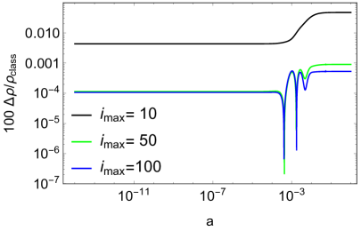
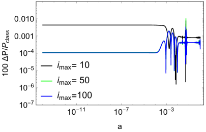
Figure 2: The percent difference between the default version of CLASS and our analytical expressions for the density (left) and the pressure (right) for 10, 50 and 100 terms (black, green and blue lines). We find that keeping 50 terms in the expansion yields an accuracy of $10^{-4}\%$ on average for the density and pressure, without affecting the performance of the code.

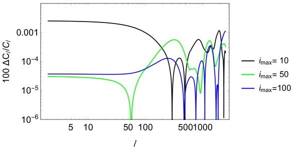
Figure 3: The percent difference in the CMB power spectrum for 10 terms in the expansion (black line), 50 terms (green line) and 100 iterations (blue line). We find that keeping 50 terms in the expansion yields an accuracy of $10^{-4}\%$ on average for the CMB spectrum, without having an impact on the performance of the code. We have smoothed the data a bit to remove the oscillatory behavior at high multipoles, but this does not affect our conclusions.

Figure 4: The percent difference in the equation of state $w(a)$ between the numerical results and the approximation of $w(a)\sim a^{-2}$ given by Eq. (3.7), for which at late times ($z<10)$, the agreement is better that $1\%$.

5 Conclusions

In this paper we presented simple but exact analytical expressions for the background evolution of the density $\rho(a)$, the pressure $P(a)$ and the average number density $n(a)$ for massive particles, both fermions and bosons. In both cases we considered the case when the particles are either relativistic or non-relativistic at the time of decoupling. We find that for non-relativistic massive particles the expressions are somewhat more cumbersome due to the presence of a double sum but in principle these results could be useful in future studies of dark matter candidates, such as WIMPs or any of the hypothetical superpartners of the leptons (sneutrino, etc.).

We also specifically tested our expressions, given by Eqs. (2.17) and (2.20) for the density and pressure respectively, in the case of massive neutrinos that are still relativistic at decoupling ($z\sim 10^{10}$), assuming one neutrino with mass of $m_{\nu}=0.06\,\textrm{eV}$. We implemented our analytical expressions in the Boltzmann code CLASS and found that by keeping 50 terms in the sum, e.g., in Eqs. (2.17) and (2.20), it is possible to achieve better than $10^{-4}\%$ accuracy with respect to the default implementation in CLASS. Our modifications in the code do not have an impact in the computational performance and avoid the involved quadrature integration scheme at the background level. Our analytical expressions provide validation for the current numerical implementations in public Boltzmann codes. By comparing CMB angular power spectra, we find the agreement between our analytical approach and the current numerical implementation is better than $10^{-4}\%$.

The main advantage of our approach is that our expressions are both exact and analytic, thus they can also provide useful intuition about the behavior of the background quantities for massive particles and how they affect the CMB. Moreover, our analytical expressions allow us to compute quantities such as the entropy density $s=\left(\rho+P\right)/T$ or the conserved number $Y=n/s$. For instance, it is possible to derive the exact behavior of the neutrino equation of state $w(a)$ at late times $(z<10)$ and show it behaves as $w\sim a^{-2}$ to better than $1\%$, in agreement with the ansatz of Ref. [23], thus demonstrating how fast massive neutrinos can become non-relativistic.

Numerical Analysis Files: The numerical codes used by the authors in the analysis of the paper and our modifications to the CLASS code will be released upon publication of the paper on the websites of the EFCLASS code here and here.

References

• [1] G. Bertone and D. Hooper, History of dark matter, Rev. Mod. Phys. 90 (2018) 045002.
• [2] Planck collaboration, Planck 2015 results. XIII. Cosmological parameters, Astron. Astrophys. 594 (2016) A13 [1502.01589].
• [3] Planck collaboration, Planck 2018 results. VI. Cosmological parameters, 1807.06209.
• [4] DES collaboration, Dark Energy Survey year 1 results: Cosmological constraints from galaxy clustering and weak lensing, Phys. Rev. D98 (2018) 043526 [1708.01530].
• [5] DES collaboration, Cosmological Constraints from Multiple Probes in the Dark Energy Survey, Phys. Rev. Lett. 122 (2019) 171301 [1811.02375].
• [6] M. Maltoni, T. Schwetz, M. A. Tortola and J. W. F. Valle, Status of global fits to neutrino oscillations, New J. Phys. 6 (2004) 122 [hep-ph/0405172].
• [7] G. L. Fogli, E. Lisi, A. Marrone and A. Palazzo, Global analysis of three-flavor neutrino masses and mixings, Prog. Part. Nucl. Phys. 57 (2006) 742 [hep-ph/0506083].
• [8] I. Esteban, M. C. Gonzalez-Garcia, A. Hernandez-Cabezudo, M. Maltoni and T. Schwetz, Global analysis of three-flavour neutrino oscillations: synergies and tensions in the determination of $\theta_{23},\delta_{CP}$, and the mass ordering, JHEP 01 (2019) 106 [1811.05487].
• [9] P. F. de Salas, D. V. Forero, C. A. Ternes, M. Tortola and J. W. F. Valle, Status of neutrino oscillations 2018: 3$\sigma$ hint for normal mass ordering and improved CP sensitivity, Phys. Lett. B782 (2018) 633 [1708.01186].
• [10] F. Capozzi, E. Lisi, A. Marrone and A. Palazzo, Current unknowns in the three neutrino framework, Prog. Part. Nucl. Phys. 102 (2018) 48 [1804.09678].
• [11] J. Lesgourgues and S. Pastor, Massive neutrinos and cosmology, Phys. Rept. 429 (2006) 307 [astro-ph/0603494].
• [12] J. Lesgourgues and S. Pastor, Neutrino cosmology and Planck, New J. Phys. 16 (2014) 065002 [1404.1740].
• [13] M. Lattanzi and M. Gerbino, Status of neutrino properties and future prospects - Cosmological and astrophysical constraints, Front.in Phys. 5 (2018) 70 [1712.07109].
• [14] K. N. Abazajian and M. Kaplinghat, Neutrino Physics from the Cosmic Microwave Background and Large-Scale Structure, Ann. Rev. Nucl. Part. Sci. 66 (2016) 401.
• [15] S. Mishra-Sharma, D. Alonso and J. Dunkley, Neutrino masses and beyond-$\mathrm{\Lambda}\mathrm{CDM}$ cosmology with lsst and future cmb experiments, Phys. Rev. D 97 (2018) 123544.
• [16] W. Hu, D. J. Eisenstein and M. Tegmark, Weighing neutrinos with galaxy surveys, Phys. Rev. Lett. 80 (1998) 5255.
• [17] D. J. Eisenstein, W. Hu and M. Tegmark, Cosmic complementarity: Joint parameter estimation from CMB experiments and redshift surveys, Astrophys. J. 518 (1999) 2 [astro-ph/9807130].
• [18] J. Lesgourgues, S. Pastor and L. Perotto, Probing neutrino masses with future galaxy redshift surveys, Phys. Rev. D 70 (2004) 045016.
• [19] C.-P. Ma and E. Bertschinger, Cosmological perturbation theory in the synchronous and conformal Newtonian gauges, Astrophys. J. 455 (1995) 7 [astro-ph/9506072].
• [20] A. Lewis, A. Challinor and A. Lasenby, Efficient computation of CMB anisotropies in closed FRW models, Astrophys. J. 538 (2000) 473 [astro-ph/9911177].
• [21] D. Blas, J. Lesgourgues and T. Tram, The Cosmic Linear Anisotropy Solving System (CLASS). Part II: Approximation schemes, Journal of Cosmology and Astro-Particle Physics 2011 (2011) 034 [1104.2933].
• [22] J. Lesgourgues and T. Tram, The Cosmic Linear Anisotropy Solving System (CLASS) IV: efficient implementation of non-cold relics, Journal of Cosmology and Astro-Particle Physics 2011 (2011) 032 [1104.2935].
• [23] M. Kunz, S. Nesseris and I. Sawicki, Constraints on dark-matter properties from large-scale structure, Phys. Rev. D94 (2016) 023510 [1604.05701].
• [24] G. Mangano, G. Miele, S. Pastor, O. Pisanti and S. Sarikas, Updated BBN bounds on the cosmological lepton asymmetry for non-zero $\theta_{13}$, Phys. Lett. B708 (2012) 1 [1110.4335].
• [25] E. Castorina, U. Franca, M. Lattanzi, J. Lesgourgues, G. Mangano, A. Melchiorri et al., Cosmological lepton asymmetry with a nonzero mixing angle $\theta_{13}$, Phys. Rev. D86 (2012) 023517 [1204.2510].
• [26] Y. Y. Y. Wong, Analytical treatment of neutrino asymmetry equilibration from flavor oscillations in the early universe, Phys. Rev. D 66 (2002) 025015.
• [27] A. D. Dolgov, S. H. Hansen, S. Pastor, S. T. Petcov, G. G. Raffelt and D. V. Semikoz, Cosmological bounds on neutrino degeneracy improved by flavor oscillations, Nucl. Phys. B632 (2002) 363 [hep-ph/0201287].
• [28] K. N. Abazajian, J. F. Beacom and N. F. Bell, Stringent constraints on cosmological neutrino anti-neutrino asymmetries from synchronized flavor transformation, Phys. Rev. D66 (2002) 013008 [astro-ph/0203442].
• [29] P. D. Serpico and G. G. Raffelt, Lepton asymmetry and primordial nucleosynthesis in the era of precision cosmology, Phys. Rev. D71 (2005) 127301 [astro-ph/0506162].
• [30] V. Barger, J. P. Kneller, P. Langacker, D. Marfatia and G. Steigman, Hiding relativistic degrees of freedom in the early universe, Phys. Lett. B569 (2003) 123 [hep-ph/0306061].
• [31] A. Cuoco, F. Iocco, G. Mangano, G. Miele, O. Pisanti and P. D. Serpico, Present status of primordial nucleosynthesis after WMAP: results from a new BBN code, Int. J. Mod. Phys. A19 (2004) 4431 [astro-ph/0307213].
• [32] T. Padmanabhan, Theoretical Astrophysics - Volume 3, Galaxies and Cosmology. Dec., 2002, 10.2277/0521562422.
• [33] I. S. Gradshteyn and I. M. Ryzhik, Table of integrals, series, and products. Elsevier/Academic Press, Amsterdam, seventh ed., 2007.
• [34] M. Abramowitz and I. A. Stegun, Handbook of mathematical functions with formulas, graphs, and mathematical tables, vol. 55 of National Bureau of Standards Applied Mathematics Series. For sale by the Superintendent of Documents, U.S. Government Printing Office, Washington, D.C., 1964.
• [35] J. Lesgourgues, G. Mangano, G. Miele and S. Pastor, Neutrino Cosmology. Cambridge University Press, 2013.
• [36] J. Lesgourgues and S. Pastor, Neutrino mass from Cosmology, Adv. High Energy Phys. 2012 (2012) 608515 [1212.6154].
• [37] V. Moll, Special Integrals of Gradshteyn and Ryzhik: the Proofs-Volume II. Chapman and Hall/CRC, 2015.
• [38] T. Bringmann and S. Hofmann, Thermal decoupling of wimps from first principles, Journal of Cosmology and Astroparticle Physics 2007 (2007) 016.
• [39] A. Sarkar, S. Das and S. K. Sethi, How late can the dark matter form in our universe?, Journal of Cosmology and Astroparticle Physics 2015 (2015) 004.