Long-lived heavy particles in neutrino mass models

Abstract

All extensions of the standard model that generate Majorana neutrino masses at the electro-weak scale introduce some “heavy” mediators, either fermions and/or scalars, weakly coupled to leptons. Here, by “heavy” we understand implicitly the mass range between a few 100 GeV up to, say, roughly 2 TeV, such that these particles can be searched for at the LHC. We study decay widths of these mediators for several different tree-level neutrino mass models. The models we consider range from the simplest $d=5$ seesaw up to $d=11$ neutrino mass models. For each of the models we identify the most interesting parts of the parameter space, where the heavy mediator fields are particularly long-lived and can decay with experimentally measurable decay lengths. One has to distinguish two different scenarios, depending on whether fermions or scalars are the lighter of the heavy particles. For fermions we find that the decay lengths correlate with the inverse of the overall neutrino mass scale. Thus, since no lower limit on the lightest neutrino mass exists, nearly arbitrarily long decay lengths can be obtained for the case where fermions are the lighter of the heavy particles. For charged scalars, on the other hand, there exists a maximum value for the decay length. This maximum value depends on the model and on the electric charge of the scalar under consideration, but can at most be of the order of a few millimeters. Interestingly, independent of the model, this maximum occurs always in a region of parameter space, where leptonic and gauge boson final states have similar branching ratios, i.e. where the observation of lepton number violating final states from scalar decays is possible.

I Introduction

The phenomenology of long-lived particles (LLPs) has received considerable attention in the literature recently. When produced at the Large Hadron Collider (LHC), LLPs can leave exotic signatures, such as, for example, displaced vertices, displaced leptons, charged tracks and others Alimena et al. (2019). All major detectors at the LHC, ALTAS, CMS and LHCb, do search for these exotics now. In addition, there are various experimental proposals, fully dedicated to LLP searches, such as MATHUSLA Chou et al. (2017); Curtin et al. (2018), CODEX-b Gligorov et al. (2017) and FASER Feng et al. (2017) or SHiP Alekhin et al. (2016). Also MoEDAL Pinfold et al. (2009), originally motivated by monopole searches, now has an LLP programme.

From the theoretical point of view there are mainly two possible motivations for introducing LLPs Curtin et al. (2018); Alimena et al. (2019): Dark matter and neutrino masses. In this paper, we will focus on the latter. We will discuss several examples of Majorana neutrino mass models and study their predictions for the decays of the new fields that these models need to introduce. For reasons explained below, we will concentrate on the mass range (0.5-2) TeV, i.e. relatively “heavy” LLPs.

The best-known example of a Majorana neutrino mass model is the simple type-I seesaw Minkowski (1977); Yanagida (1979); Mohapatra and Senjanovic (1980). Here, two (or more) copies of fermionic singlets, $N$, are added to the standard model. These states, sometimes called right-handed neutrinos, sterile neutrinos, heavy neutrinos or also “heavy neutral leptons” (HNL) will mix with the SM neutrinos after electro-weak symmetry breaking. Standard model charged and neutral current interactions then yield a small, but non-zero production rate for these nearly singlet states proportional to $\sum_{\alpha}|U_{\alpha i}|^{2}$, where $U_{\alpha i}$ is the mixing angle between the neutrino of flavour $\alpha=e,\mu,\tau$ and the sterile neutrino eigenstate, $N_{i}$. Recent phenomenological studies assessing the LHC sensitivity with displaced vertices to light sterile neutrinos in various models have been published in Helo et al. (2014); Deppisch et al. (2018); Helo et al. (2018); Nemevšek et al. (2018); Lara et al. (2018); Dev et al. (2017); Cottin et al. (2018, 2019); Dercks et al. (2019), see also the review Alimena et al. (2019). The large statistics expected at the high-luminosity LHC should allow to probe mixing angles down to roughly $\sum_{\alpha}|U_{\alpha i}|^{2}\sim 10^{-9}$, for masses below $m_{N_{1}}\sim 25$ GeV Cottin et al. (2018) at ATLAS (or CMS) and below $m_{N_{1}}\sim 5$ GeV at MATHUSLA Helo et al. (2018); Curtin et al. (2018).

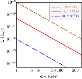
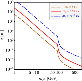
For the simplest seesaw type-I one can estimate an upper bound on the decay length for a given sterile neutrino mass $m_{N}$, assuming that the corresponding state contributes a certain amount to the active neutrino mass(es). This estimate is shown in fig. (1). Here, we have used the well-known Casas-Ibarra approximation Casas and Ibarra (2001) to reparametrize the seesaw. For the plot we fix the neutrino oscillation data at their best fit point (b.f.p.) values, choose normal hierarchy and assume that the matrix ${\cal R}$ is trivial. We then choose three different example values for the lightest neutrino mass. Note that $m_{\nu_{1}}=1$ eV is experimentally excluded, both from cosmology Aghanim et al. (2018) and from double beta decay searches Gando et al. (2016); Agostini et al. (2018) and is shown only for the sake of demonstrating the parameter dependence. The choice of $m_{\nu_{1}}=0.05$ eV is motivated by the atmospheric neutrino mass scale. The sterile neutrino widths have been calculated with the formulas given in Atre et al. (2009); Bondarenko et al. (2018). The decay lengths shown are to be understood as upper bounds, since choosing a non-trivial ${\cal R}$ will lead in general to larger mixing and thus to smaller decay lengths.

As fig. (1) shows, for masses $m_{N_{1}}$ above, say $m_{W}$, decay lengths drop quickly to values below $c\tau\sim 1$ mm, except for the region of parameter space, where the lightest neutrino mass is much smaller than $m_{\nu_{1}}=0.05$ eV. Comparing to the plot on the left of the figure, however, shows that such small values of $m_{\nu_{1}}$ correspond to very small values of the mixing angle squared, $\sum_{\alpha}|U_{\alpha 1}|^{2}$. The production rates of long-lived “heavy” steriles, i.e. with $m_{N}\raise 1.29167pt\hbox{$\;>$\kern-7.5pt\raise-4.73611pt\hbox{$\sim\;$}}100$ GeV, is therefore expected to be unmeasurably small in models based in seesaw type-I.

Figure 1: Naive estimate of the mixing angle (left) and decay length (right) of the lightest sterile neutrino in a type-I seesaw for a given value of the lightest active neutrino mass as function of the sterile neutrino mass, $m_{N_{1}}$.

The situation can be very different in other electro-weak scale model of neutrino masses. The principle idea is rather simple. Consider, for example, the so-called seesaw type-III Foot et al. (1989). Here, an electro-weak triplet fermion is introduced, usually denoted by $\Sigma$. Production at the LHC can proceed, for example, via $pp\to W^{\pm}\to\Sigma^{0}\Sigma^{\pm}$, i.e. with electro-weak strength. The decays $\Sigma^{0}\to W^{\pm}+l_{\alpha}^{\mp}$ and $\Sigma^{\pm}\to W^{\pm}+\nu_{\alpha}$ are, however, again mixing suppressed Franceschini et al. (2008), as discussed above for the case of the type-I seesaw. Thus, very small decay widths do not necessarily imply small producion rates in general. In this paper, we will study this idea in some detail, considering a variety of different Majorana neutrino models. Note that all models we consider will produce neutrino masses at tree-level.

Majorana neutrino masses can be generated from operators of odd dimensions, starting from $d=5$. One can write these $\Delta L=2$ operators as:

$${\cal O}_{\Delta L=2}=\frac{c_{\alpha\beta}}{\Lambda^{2n+1}}L_{\alpha}L_{\beta}HH(HH^{\dagger})^{n}.$$ (1)

Here, $c_{\alpha\beta}$ is some dimensionless coefficient and $n=0$ corresponds to the well-known Weinberg operator Weinberg (1979). The Weinberg operator has three different independent contractions Ma (1998), which correspond - at tree-level - to the three classical seesaws Minkowski (1977); Yanagida (1979); Mohapatra and Senjanovic (1980); Schechter and Valle (1980); Foot et al. (1989). Less known are the models at $d>5$. Reference Bonnet et al. (2009) presented a complete deconstruction of the $d=7$ operator at tree-level. However, most of the ultra-violet completions (or “models”) found in Bonnet et al. (2009) require additional symmetries, beyond those of the standard model, in order to avoid the $d=5$ seesaw contributions. On the other hand, there is one $d=7$ model, first presented in Babu et al. (2009), for which all $d=5$ (tree-level) contributions are automatically absent. Following Aristizabal Sierra et al. (2015); Cepedello et al. (2018); Anamiati et al. (2018) we will call such models “genuine” and in our numerical calculations we will consider only genuine models. In addition to the $d=7$ model Babu et al. (2009), called BNT model below, we will choose one model at $d=9$ and one at $d=11$ each. These two models have been first discussed in Anamiati et al. (2018).

Charged particles, be they fermions or scalars, would have been seen at LEP, if their masses are below (80-115) GeV Tanabashi et al. (2018), with the exact number depending on the decay modes and nature of the particle under consideration. Thus, none of the models we consider in this paper can work with an overall mass scale below roughly 100 GeV. Also the LHC will provide important constraints on all our models. Here, however, the situation is much more complicated. Consider for example the seesaw type-II Schechter and Valle (1980). Here, a scalar triplet is added to the standard model and ATLAS has searched for this state in $pp\to\Delta^{++}\Delta^{--}\to 4\ell$ Aaboud et al. (2018). The limits are in the range (770 - 870) GeV, depending on the lepton flavour, assuming Br($\Delta^{\pm\pm}\to\ell^{\pm}_{\alpha}\ell^{\pm}_{\beta}$) equal to 1 (for $\alpha,\beta=e,\mu$). CMS Collaboration (2017) has studied both pair- and associated production of scalars and obtained limits for leptonic final states similar to the ones by ATLAS. ATLAS has also considered $pp\to\Delta^{++}\Delta^{--}\to 4W$. However, lower limits for a $\Delta^{++}$ decaying to gauge bosons are currently only of order 220 GeV Aaboud et al. (2019). For the fermions of seesaw type-III CMS quotes a lower limit of $\sim 840$ GeV Sirunyan et al. (2017), assuming a “flavour democratic” decay, i.e. equal branching ratios to electrons, muons and taus. Weaker limits would be obtained for states decaying mostly to taus. Note that this search Sirunyan et al. (2017) assumes that all decays are prompt. For the more complicated final states of our $d>5$ models no dedicated LHC searches exist so far, but one can expect that current sensitivities should be somewhere between ($0.5-1$) TeV, depending on whether one considers scalars or fermions. The high-luminosity LHC will of course be able to considerably extend this mass range. Thus, we will consider (roughly) the mass range (0.5-2) TeV in this paper.

The rest of this paper is organized as follows. We will give the particle content and the Lagrangians of the models used in the numerical parts of this paper in section II. We divide then the numerical discussion into two sections. First, in section III we calculate the decays of exotic fermions, while section IV discusses the decays of exotic scalars. In both sections, the main emphasis is on identifying the regions in parameter space, where the decay widths of the lightest exotic particles are sufficiently small that experiments will be able to find displaced vertices or charged tracks, depending on whether the particles considered are neutral or charged. We then close with a short summary and discussion.

II Models

In this section we will discuss the basics of the different neutrino mass models that we consider in the numerical part of this work. All models studied here generate neutrino masses at tree-level. The lowest order operator to generate Majorana neutrino masses is the Weinberg Weinberg (1979) operator at $d=5$, which at tree-level can be realized in three different ways. For higher dimensional operators generating neutrino masses, we will consider one example model each at $d=7$, $d=9$ and $d=11$. The models we selected are all “genuine” models in the sense that they give automatically the leading contribution to the neutrino mass without resorting to any additional symmetry beyond the SM ones.

To fix notation, with the exception of the classical three seesaw mediators (see below), we will use ${\bf R}_{Y}$ for $SU(2)_{L}$ representations with hypercharge $Y$ and add a superscript $F$ or $S$ to denote fermions and or scalars. For example, ${\bf 3}^{F}_{1}$ is a fermionic triplet with hypercharge one. The different components of these representations are then written classified by their electric charge. For example, ${\bf 3}^{F}_{1}$ is written in components as ($F^{++}_{3},F^{+}_{3},F^{0}_{3}$), where we exchange ${\bf R}$ and $F$ to avoid confusion between multiplets and charge eigenstates.

II.1 $d=5$

Figure 2: Tree-level neutrino mass diagrams for the $d=5$ Weinberg operator. These are the three well-known variants of the seesaw, from left to right: Type-I, -II and -III.

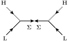
At $d=5$ there are three models that generate neutrino masses at tree-level. These are known as seesaw type-I, type-II and type-III in the literature. Seesaw type-I adds fermionic singlets to the standard model (SM), ${\bf 1}^{F}_{0}\equiv N$. Type-II adds a scalar triplet to the SM, ${\bf 3}^{S}_{1}\equiv\Delta$, while type-III uses fermionic triplets, ${\bf 3}^{F}_{0}\equiv\Sigma$. For these three fields the names $N$, $\Delta$ and $\Sigma$ are customary in the literature; we follow this convention. The neutrino mass diagrams for the three classical seesaws are shown in fig. 2.

These three models are very well-known and we give the Lagrangians here only to fix the notation. The Lagrangian for type-I seesaw is given by:

$${\cal L}={\cal L}^{\rm SM}+Y_{\nu}{\overline{L}}H^{\dagger}N+\frac{1}{2}M_{N}{\overline{N}^{c}}N.$$ (2)

Here, $M_{N}$ is a matrix with eigenvalues $m_{N_{i}}$. For the seesaw type-II one has:

$${\cal L}={\cal L}^{\rm SM}+Y_{\Delta}{\overline{L}^{c}}\Delta L+\mu_{\Delta}H\Delta^{\dagger}H+m_{\Delta}^{2}|\Delta|^{2}\cdots$$ (3)

Here, we neglected to write down other terms in the scalar potential which are not directly relevant for neutrino mass generation. Recall, that the term proportional to $\mu_{\Delta}$ induces a vacuum expectation value for the triplet: $v_{\Delta}\simeq\mu_{\Delta}\frac{v^{2}}{m_{\Delta}^{2}}$. Here, $v$ is the standard model Higgs vev. Finally, for type-III we write:

$${\cal L}={\cal L}^{\rm SM}+Y_{\Sigma}{\overline{L}}H^{\dagger}\Sigma+\frac{1}{2}M_{\Sigma}\Sigma\Sigma.$$ (4)

In these equations we have suppressed generation indices. Recall, however, that for type-I and type-III seesaw there is one non-zero active neutrino mass per generation of singlet/triplet field added. Thus, for these cases at least two copies of extra fermions are needed. In our numerical studies we always use three copies of extra fermions. All matrices $Y_{\nu}$, $Y_{\Delta}$, $Y_{\Sigma}$ and $M_{N}$ and $M_{\Sigma}$ are then ($3,3$) matrices.

For setting up the notation, here we give also the mass matrices for the neutral and charged fermions in seesaw type-III. The neutral fermion mass matrix, in the basis ($\nu,\Sigma^{0}$), is given by

$$M^{0}=\left(\begin{array}[]{cc}0&\frac{v}{\sqrt{2}}Y_{\Sigma}\\ \frac{v}{\sqrt{2}}Y_{\Sigma}^{T}&M_{\Sigma}\end{array}\right),$$ (5)

while the charged fermion mass matrix, in the basis ($l,\Sigma^{-}$), is:

$$M^{+}=\left(\begin{array}[]{cc}\frac{v}{\sqrt{2}}Y_{l}&\frac{v}{\sqrt{2}}Y_{\Sigma}\\ 0&M_{\Sigma}\end{array}\right).$$ (6)

Note that the mixing between heavy and light states in both, the neutral and the charged sectors, is to first approximation given by $(Y_{\Sigma}v).M_{\Sigma}^{-1}$.

II.2 $d=7$

Figure 3: Tree-level neutrino mass diagram for the genuine $d=7$ model Babu et al. (2009).

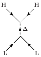
The model we consider at $d=7$ first appeared in reference  Babu et al. (2009); we therefore call it the BNT model. The phenomenology of this model has been studied also in Ghosh et al. (2018a, b). In the BNT model, two kinds of fields are added to the SM; a scalar quadruplet, ${\bf 4}^{S}_{3/2}$ and a fermionic triplet, ${\bf 3}^{F}_{1}$, together with its vector partner ${\bf 3}^{F}_{-1}$. The Lagrangian of this model contains the terms

$${\cal L}={\cal L}^{\rm SM}+Y_{\Psi}LH^{\dagger}{\bf 3}^{F}_{1}+Y_{\overline{\Psi}}{\bf 4}^{S}_{3/2}{\bf 3}^{F}_{-1}L+M_{\bf 3}{\bf 3}^{F}_{1}{\bf 3}^{F}_{-1}+m_{4}^{2}|{\bf 4}^{S}_{3/2}|^{2}+\lambda_{5}HHH({\bf 4}^{S}_{3/2})^{\dagger}+\cdots,$$ (7)

Here, we have again written only those terms that appear in the diagram for neutrino masses, see fig. (3). The last term in eq. (7) induces a vacuum expectation value (vev) for the neutral component of the ${\bf 4}^{S}_{3/2}$, even for $m_{4}^{2}\geq 0$. Roughly one can estimate

$$v_{\bf 4}\simeq-\lambda_{5}\frac{v^{3}}{m_{4}^{2}}.$$ (8)

The SM $\rho$ parameter Tanabashi et al. (2018) requires that this vev is small, we estimate $v_{\bf 4}\raise 1.29167pt\hbox{$\;<$\kern-7.5pt\raise-4.73611pt\hbox{$\sim\;$}}3.5$ GeV.

In the calculation of the neutrino mass matrix, one can use eq. (8) to rewrite the full neutral fermion mass matrix, in the basis ($\nu,F^{0}_{3},{\overline{F}}^{0}_{3}$):

$$M^{0}=\left(\begin{array}[]{ccc}0&\frac{v}{\sqrt{2}}Y_{\Psi}&\frac{v_{\bf 4}}{\sqrt{2}}Y_{\overline{\Psi}}^{T}\\ \frac{v}{\sqrt{2}}Y_{\Psi}^{T}&0&M_{\bf 3}\\ \frac{v_{\bf 4}}{\sqrt{2}}Y_{\overline{\Psi}}&M_{\bf 3}^{T}&0\end{array}\right).$$ (9)

This matrix has the same structure as found in the so-called “linear seesaw” models Akhmedov et al. (1996a, b). The light neutrino masses are therefore given approximately as

$$m_{\nu}\simeq\frac{1}{2}\left(Y_{\Psi}M_{\bf 3}^{-1}Y_{\overline{\Psi}}^{T}+Y_{\overline{\Psi}}M_{\bf 3}^{-1}Y_{\Psi}^{T}\right)vv_{\bf 4}.$$ (10)

Note the additional suppression of the neutrino masses by a factor ($v_{\bf 4}/v$) compared to the standard seesaw.

The charged fermion mass matrix in the basis $(l,F_{3}^{-})$, is given by:

$$M^{+}=\left(\begin{array}[]{c c}\frac{vY_{e}}{\sqrt{2}}&-\frac{v}{2}Y_{\Psi}\\ 0&M_{\bf 3}\end{array}\right)$$ (11)

Note that the neutrino masses require $Y_{\Psi}$ and/or $Y_{\overline{\Psi}}$ to be small, see eq. (10). Thus, unless there is a large hierarchy imposed on the couplings $Y_{\Psi}$ and $Y_{\overline{\Psi}}$, one expects the mixing between the heavy charged states and the charged leptons to be small.

II.3 $d=9$

Figure 4: Tree-level neutrino masses diagrams for two different higher-dimensional neutrino mass models. A $d=9$ diagram to the left and a $d=11$ diagram to the right.

As shown in Anamiati et al. (2018), there are two genuine tree-level neutrino mass models at $d=9$. model-I is the simpler variant, since it contains only three new fermions, ${\bf 3}_{1}^{F}$, ${\bf 4}_{1/2}^{F}$ and ${\bf 5}_{0}^{F}$, together with their vector partners. The Lagrangian of the model can be written as:

$${\cal L}={\cal L}_{SM}+{\cal L}_{Yuk}+{\cal L}_{mass},$$ (12)

where

$${\cal L}_{Yuk} =Y_{\Psi}\,L{\bf 3}_{1}^{F}H^{\dagger}+{\overline{Y}}_{\bf 34}\,{\bf 3}_{-1}^{F}{\bf 4}_{1/2}^{F}H+Y_{\bf 34}\,{\bf 3}_{1}^{F}{\bf 4}_{-1/2}^{F}H^{\dagger}$$ (13)

$$\quad+{\overline{Y}}_{\bf 45}\,{\bf 4}_{1/2}^{F}{\bf 5}_{0}^{F}H^{\dagger}+Y_{\bf 45}\,{\bf 4}_{-1/2}^{F}{\bf 5}_{0}^{F}H$$

and

$${\cal L}_{mass}=M_{\bf 3}{\bf 3}_{1}^{F}{\bf 3}_{-1}^{F}+M_{\bf 4}{\bf 4}_{1/2}^{F}{\bf 4}_{-1/2}^{F}+M_{\bf 5}{\bf 5}_{0}^{F}{\bf 5}_{0}^{F}.$$ (14)

The mass matrix for the neutral states, in the basis ($\nu,F^{0}_{3},{\overline{F}}^{0}_{3},F^{0}_{4},{\overline{F}}^{0}_{4},F^{0}_{5}$), is given by

$$M^{0}=\left(\begin{array}[]{cccccc}0&\frac{v}{\sqrt{2}}Y_{\Psi}&0&0&0&0\\ \frac{v}{\sqrt{2}}Y_{\Psi}^{T}&0&M_{\bf 3}&0&\frac{v}{\sqrt{6}}Y_{\bf 34}&0\\ 0&M_{\bf 3}^{T}&0&\frac{v}{\sqrt{6}}{\overline{Y}}_{\bf 34}&0&0\\ 0&0&\frac{v}{\sqrt{6}}{\overline{Y}}_{\bf 34}^{T}&0&M_{\bf 4}&\frac{v}{2}{\overline{Y}}_{\bf 45}\\ 0&\frac{v}{\sqrt{6}}Y_{\bf 34}^{T}&0&M_{\bf 4}^{T}&0&\frac{v}{2}Y_{\bf 45}\\ 0&0&0&\frac{v}{2}{\overline{Y}}_{\bf 45}^{T}&\frac{v}{2}Y_{\bf 45}^{T}&M_{\bf 5}\\ \end{array}\right).$$ (15)

This matrix has an iterated seesaw structure, as can be understood also from the neutrino mass diagram shown in fig. (4), to the left. Repeatedly applying the seesaw approximation, the light neutrino mass matrix can be roughly estimated as:

$$m_{\nu}\sim\frac{1}{48}Y_{\Psi}M_{\bf 3}^{-1}{\overline{Y}}_{\bf 34}M_{\bf 4}^{-1}Y_{\bf 45}M_{\bf 5}^{-1}Y_{\bf 45}^{T}(M_{\bf 4}^{T})^{-1}{\overline{Y}}_{\bf 34}^{T}(M_{\bf 3}^{T})^{-1}Y_{\Psi}^{T}v_{SM}^{6}+\cdots$$ (16)

Here, we have neglected terms proportional to $Y_{\bf 34}$ and ${\overline{Y}}_{\bf 45}$, since they are formally of higher order (i.e. $d=11,13$ contributions to $m_{\nu}$). Note that, for generating non-zero neutrino masses all matrices $Y_{\Psi}$, ${\overline{Y}}_{\bf 34}$ and $Y_{\bf 45}$ must contain non-zero entries, while non-zero terms for $Y_{\bf 34}$ and ${\overline{Y}}_{\bf 45}$ are not required.

Finally, for this model, the charged fermion matrix, in the basis $(l,F_{3}^{-},F_{4}^{-},(F_{4}^{+})^{c},F_{5}^{-})$, is given by:

$$M^{+}=\begin{pmatrix}\frac{v}{\sqrt{2}}Y_{e}&-\frac{v}{2}Y_{\Psi}&0&0&0\\ 0&M_{\bf 3}&\frac{1}{\sqrt{3}}v{\overline{Y}}_{\bf 34}&0&0\\ 0&\frac{1}{\sqrt{3}}v{Y}_{\bf 34}^{T}&0&M_{\bf 4}&-\frac{v}{2\sqrt{2}}{\overline{Y}}_{\bf 45}\\ 0&0&M_{\bf 4}&0&\frac{\sqrt{3}}{2\sqrt{2}}vY_{\bf 45}\\ 0&0&-\frac{\sqrt{3}}{2\sqrt{2}}v{\overline{Y}}_{\bf 45}^{T}&\frac{v}{2\sqrt{2}}Y_{\bf 45}^{T}&-M_{\bf 5}\end{pmatrix}.$$ (17)

II.4 $d=11$

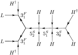
Also at $d=11$ level there are two genuine neutrino mass models at tree-level Anamiati et al. (2018). The neutrino mass diagram of model-I is shown in fig. 4, to the right. Again, we have chosen this model over model-II since it has the smaller particle content. Model-I needs one exotic fermion, ${\bf 3}^{F}_{1}$ (plus vector partner) and three different scalars: ${\bf 5}^{S}_{2}$, ${\bf 5}^{S}_{1}$ and ${\bf 3}^{S}_{0}$, Here we write down only the Lagrangian terms important for generating neutrino masses:

$${\cal L} \propto\lambda_{55}({\bf 5}_{2}^{S})^{\dagger}{\bf 5}_{1}^{S}HH+\lambda_{53}({\bf 5}_{1}^{S})^{\dagger}{\bf 3}_{0}^{S}HH+\mu_{3}{\bf 3}_{0}^{S}HH^{\dagger}+m_{3}^{2}|{\bf 3}_{0}^{S}|^{2}$$ (18)

$$\quad+m_{5_{1}}^{2}|{\bf 5}_{1}^{S}|^{2}+m_{5_{2}}^{2}|{\bf 5}_{2}^{S}|^{2}+Y_{\Psi}L{\bf 3}_{1}^{F}H^{\dagger}+Y_{3}{\bf 3}_{1}^{F}{\bf 3}_{1}^{F}({\bf 5}_{2}^{S})^{\dagger}+Y_{\overline{3}}{\bf 3}_{-1}^{F}{\bf 3}_{-1}^{F}{\bf 5}_{2}^{S}+M_{\bf 3}{\bf 3}_{-1}^{F}{\bf 3}_{1}^{F}.$$

The neutral components of the scalars ${\bf 3}_{0}^{S}$, ${\bf 5}_{1}^{S}$ and ${\bf 5}_{2}^{S}$ will acquire vevs, $v_{3}$, $v_{51}$ and $v_{52}$ respectively. Solving the tadpole equations gives:

$$v_{3} = \frac{\mu_{3}v^{2}(16m_{5_{1}}^{2}m_{5_{2}}^{2}-\lambda_{55}^{2}v^{4})}{(-32m_{3}^{2}m_{5_{1}}^{2}m_{5_{2}}^{2}+2\lambda_{55}^{2}m_{3}^{2}v^{4}+4\lambda_{53}^{2}m_{5_{2}}^{2}v^{4})}\sim-\frac{\mu_{3}v^{2}}{2m_{3}^{2}},$$ (19)

$$v_{51} = -\frac{2\sqrt{2}\lambda_{53}m_{5_{2}}^{2}\mu_{3}3v^{4}}{(-16m_{3}^{2}m_{5_{1}}^{2}m_{5_{2}}^{2}+\lambda_{55}^{2}m_{3}^{2}v^{4}+2\lambda_{53}^{2}m_{5_{2}}^{2}v^{4})}\sim\frac{\lambda_{53}\mu_{3}v^{4}}{4\sqrt{2}m_{3}^{2}m_{5_{1}}^{2}},$$ (20)

$$v_{52} = -\frac{\lambda_{53}\lambda_{55}\mu_{3}v^{6}}{\sqrt{2}(-16m_{3}^{2}m_{5_{1}}^{2}m_{5_{2}}^{2}+\lambda_{55}^{2}m_{3}^{2}v^{4}+2\lambda_{53}^{2}m_{5_{2}}^{2}v^{4})}\sim\frac{\lambda_{53}\lambda_{55}\mu_{3}v^{6}}{16\sqrt{2}m_{3}^{2}m_{5_{1}}^{2}m_{5_{2}}^{2}}.$$ (21)

Again, all these vevs have to be numerically small, due to the precise measurements for the $\rho$ parameter Tanabashi et al. (2018). Eq. (21) allows to trade the parameters of the scalar sector for $v_{52}$ in the calculation of the neutral fermion mass matrix. The resulting mass matrix, in the basis ($\nu,F^{0}_{3},{\overline{F}}^{0}_{3}$), is given by:

$$M^{0}=\left(\begin{array}[]{ccc}0&\frac{v}{\sqrt{2}}Y_{\Psi}&0\\ \frac{v}{\sqrt{2}}Y_{\Psi}^{T}&\frac{1}{\sqrt{2}}Y_{3}v_{52}&M_{\bf 3}\\ 0&M_{\bf 3}^{T}&\frac{1}{\sqrt{2}}Y_{\overline{3}}v_{52}\end{array}\right).$$ (22)

This matrix is of the same form as the one found in “inverse seesaw” models Mohapatra and Valle (1986). A simple estimate for the neutrino mass from the diagram on the right in fig. 4 gives:

$$m_{\nu}\simeq\frac{v_{52}v^{2}}{2\sqrt{2}}Y_{\Psi}M_{\bf 3}^{-1}Y_{\overline{3}}(M^{T}_{\bf 3})^{-1}Y_{\Psi}^{T}.$$ (23)

We have implemented all models discussed in this section in SARAH Staub (2013, 2014). In all cases, we use three generation of the new fermion fields, although we mention that neutrino oscillation fits in principle could be done with less copies of fields. These implementations allow to generate automatically SPheno routines Porod (2003); Porod and Staub (2012) for the numerical evaluation of mass spectra, mixing matrices, 2-body and fermionic 3-body decays. SARAH also allows to generate model files for MadGraph Alwall et al. (2007, 2011, 2014), which we use for the numerical calculation of several multi-particle final state decay widths, see section IV. Finally, we use the package SSP Staub et al. (2012) to perform parameter scans.

III Fermionic decays

In this section, we will study the decay of the heavy fermionic fields that mediate the $d=5$, $d=7$ and $d=9$ tree-level neutrino mass generation mechanisms described in the last section. For each model, we identify the most interesting part of the parameter space where the heavy mediator field has an experimentally measurable decay length. In this section, we always assume that the exotic scalars of the different models are heavier than the fermions, such that they do not appear in the decay chains.

The CMS search for the fermions of the seesaw type-III Sirunyan et al. (2017), will give limits on all models we are discussing in this section too, as long as the decays of the fermions are prompt. The limits derived in Sirunyan et al. (2017), depend heavily on the lepton flavour the heavy fermion decays to. Varying the branching ratios to $e,\mu,\tau$ between zero and one, limits in the range (390-930) GeV were found. The lower end of this range corresponds to fermions decaying to taus, while the upper end corresponds to fermions decaying 100 % to muons. We expect that limits on the fermionic states of the other models we are considering should lie in a similar range. However, we stress that here we are mostly interested in long-lived fermions, so the search Sirunyan et al. (2017) is not directly applicable.

Let us start the discussion with some general observations. In any of the different models, the heavy fermions $F$ will decay to a light fermion $f$ plus a boson $V$ as $F\rightarrow f+V$. Here, $V$ can be either a $W$, a $Z^{0}$ or a Higgs boson, $h$. Consider, for example, the charged-current vertex. In the limit where the heavy fermion mass is much larger than the $W$ mass the decay width for $\Gamma(F^{0}\rightarrow f^{-}+W^{+})$ is described approximately by:

$$\Gamma(F^{0}_{i}\rightarrow W^{+}+l^{-}_{j})\sim\frac{1}{32\pi}|V_{ij}|^{2}\frac{m_{F}^{3}}{m_{W}^{2}},\quad V_{ij}=\frac{g}{\sqrt{2}}U_{\nu_{i\alpha}}U^{\dagger}_{l_{\alpha j}}$$ (24)

Here, $U_{\nu}$ diagonalizes the mass matrix of the neutral states, and $U_{l}$ diagonalizes the mass matrix of the charged states. Both, in the SM and in seesaw type-I, we can choose a basis where $U_{l}$ is diagonal, but in more general models this is not the case. Off-diagonal entries, connecting heavy and light states, will be suppressed in both, $U_{\nu}$ and $U_{l}$, with the suppression usually of the same order in both matrices. Typically one finds $|V_{ij}|^{2}\sim\frac{m_{\nu}}{m_{F}}$, for heavy-to-light transitions. Similar suppression factors are found for final states involving $Z$ and $h$ bosons. This explains the smallness of the heavy particle widths qualitatively. In our numerical analysis, however, we always use SPheno Porod (2003); Porod and Staub (2012), which diagonalizes all mass matrices exactly.

III.1 $d=5$

In seesaw models, both, $U_{l}$ and $U_{\nu}$, are in general larger matrices than $(3\times 3)$. In seesaw type-I $U_{l}$ and $U_{\nu}$ are $(3\times 3)$ and $(6\times 6)$ matrices respectively. For an estimation of the decay length for a sterile neutrino in seesaw type-I see the introduction. Here, we will discuss the phenomenologically more interesting case of the seesaw type-III.

For seesaw type-III, both $U_{\nu}$ and $U_{l}$ are $(6\times 6)$ matrices. We can express $Y_{\Sigma}$ in terms of the measured neutrino masses and angles, using the Casas-Ibarra parametrization Casas and Ibarra (2001):

$$Y_{\Sigma}=\frac{i}{v}\sqrt{\hat{M}_{\Sigma}^{-1}}{\cal R}\sqrt{{\hat{m}}_{\nu}}U_{\nu}^{\dagger}.$$ (25)

Here, as usual, ${\hat{M}_{\Sigma}}$ is diagonal, ${\cal R}$ is an arbitrary orthogonal matrix, ${\hat{m}}_{\nu}$ are the light neutrino mass eigenvalues and $U_{\nu}$ is assumed to be the mixing matrix, as measured in oscillation experiments. Note, that since $U_{l}$ is not diagonal in general, the latter is an approximation. However, mixing between heavy and light sectors are of order $(Y_{\Sigma}v).M_{\Sigma}^{-1}$, for both neutral and charged fermions, see section II. Corrections to eq. (25) are therefore usually small. We note that this is particularly so in the region of parameter space, in which we are interested in: Large decay lengths require small values of $(Y_{\Sigma}v).M_{\Sigma}^{-1}$. We thus put in the numerical scans ${\cal R}=1$. Smaller decay lengths than the ones shown below could be obtained, for a matrix ${\cal R}$ with complex angles with large absolute values $|z|^{2}\gg 1$.

Figure 5: Left: Decay length for the neutral and charged components of the fermionic triplet $\Sigma$, as function of $m_{\Sigma}$, for several fixed choices of the lightest neutrino mass. The figure demonstrates that neutral and charged components of the fermionic triplet have nearly identical decay lengths. The gray band correspond to $c\tau>1$ mm. Right: Decay length for the neutral component of the fermionic triplet versus the lightest neutrino mass $m_{\nu_{1}}$. Solid (dashed) lines correspond to the case where $m_{\Sigma}=1$ TeV ($m_{\Sigma}=500$ GeV.)

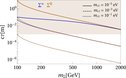
Example calculations for the decay lengths of the heavy fermions are shown in fig. 5. Here and in all plots shown below, unless noted otherwise, we fix the neutrino oscillation data at their best fit point (b.f.p.) values, choose normal hierarchy and assume that the matrix ${\cal R}$ is trivial. The plot to the left shows the decay length, $c\tau$, for the neutral and charged components of the fermionic triplet $\Sigma$, as function of $m_{\Sigma}$, for several fixed choices of the lightest neutrino mass. Recall that $m_{\Sigma}$ below 390 GeV has already been ruled out by CMS Sirunyan et al. (2017). Neutral and charged components of the fermionic triplet have nearly identical decay lengths in the region of parameter space where $c\tau$ is smaller than roughly $c\tau\simeq 6$ cm. However, while $\Sigma^{0}$ can have much larger decay lengths, for $\Sigma^{+}$ there is an upper limit on $c\tau$ of this order. This upper limit is due to the decays $\Sigma^{+}\to\Sigma^{0}+\pi^{+}$. Different from the decays to standard model particles, the decays $\Sigma^{+}\to\Sigma^{0}+\pi^{+}$ are not suppressed by the smallness of the neutrino masses. Instead, because the masses of $\Sigma^{+}$ and $\Sigma^{0}$ are not exactly degenerate, once 1-loop corrections are taken into account, there is a small but non-zero decay width $\Gamma(\Sigma^{+}\to\Sigma^{0}+\pi^{+})\propto(\Delta M)^{3}$, as pointed out first in Franceschini et al. (2008). Note that, $(\Delta M)\sim 160$ MeV, in the limit $m_{\Sigma}\gg m_{Z}$, leading to a maximal $c\tau$ of order 6 cm for the charged state.

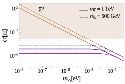
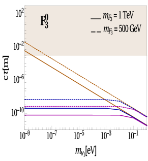
The plot on the right shows the decay length for the neutral component of the fermionic triplet versus the lightest neutrino mass $m_{\nu_{1}}$. Here, we show two cases, fixing the mass of lightest $\Sigma$ to $500$ GeV (dashed lines) and $1$ TeV (solid lines). Orange, blue and magenta solid lines correspond to the cases where the lightest of the three neutral triplets $\Sigma_{i}^{0}$ is the one associated with $m_{\nu_{i}}$, $i=1,2,3$, where for normal hierarchy we have $m_{\nu_{i}}=\{m_{\nu_{1}},\sqrt{\Delta m_{\odot}^{2}+m_{\nu_{1}}^{2}}$, $\sqrt{\Delta m_{\rm Atm}^{2}+m_{\nu_{1}}^{2}}\}$. Blue and magenta lines are always in a region with $c\tau$ below 1 mm, so one does not expect that at the LHC a displaced vertex for these particles can be seen. However, for the case where the lightest $\Sigma$ is the one associated to $m_{\nu_{1}}$, for small values of $m_{\nu_{1}}$ the decay length can be arbitrarily large. This different behaviour is easily understood: Solar and atmosperic neutrino mass squared differences require a minimum value for $m_{\nu_{2}}\raise 1.29167pt\hbox{$\;>$\kern-7.5pt\raise-4.73611pt\hbox{$\sim\;$}}8.5$ meV and $m_{\nu_{3}}\raise 1.29167pt\hbox{$\;>$\kern-7.5pt\raise-4.73611pt\hbox{$\sim\;$}}50$ meV, while for $m_{\nu_{1}}$ there is no lower limit experimentally. For example, for masses of $m_{\Sigma}$ to $500$ GeV (1 TeV), $c\tau\gtrsim 10^{-3}$ meter as long as the lightest neutrino mass is $m_{\nu_{1}}\lesssim 10^{-3}$ eV ($m_{\nu_{1}}\lesssim 2\times 10^{-4}$) eV. For very small values of $m_{\nu_{1}}$ the neutral fermions become quasi-stable on LHC detector time scales, thus the displaced vertex signal disappear (only missing energy is seen from $\Sigma^{0}$). In this same part of parametric space $\Sigma^{+}$ will have a decay length $c\tau\sim 6$ cm, thus leaving a charged track signature inside the detector.

III.2 $d=7$

We now turn to a discussion of the fermions in the BNT model. For this model, the full neutral ($9\times 9$) and charged ($6\times 6$) fermion mass matrices are given in eq. (9) and (11). As shown in eq. (10), for the BNT model neutrino masses are essentially given by a linear seesaw. Here, there are two independent Yukawa couplings, denoted by $Y_{\Psi}$ and $Y_{\overline{\Psi}}$. This gives, in general, more parametric freedom to fit neutrino oscillation data then can be described with the standard Casas-Ibarra parametrization. A completely general description for the neutrino mass fit for any Majorana neutrino mass model has recently been given in Cordero-Carrión et al. (2019a, b).

However, here as everywhere else in this paper, we will be interested again in the parameter region, where the decay length of the heavy fermions is maximized. To start the discussion, consider the mixing matrices $U_{\nu}$ and $U_{l}$. For neutrinos one can estimate $U_{\nu}^{H-L}\propto v(Y_{\Psi}\pm Y_{\overline{\Psi}}).M_{\bf 3}^{-1}$, where $H-L$ indicates that we are considering here only the off-diagonal parts of $U_{\nu}$, describing heavy-light mixing. $U_{l}^{H-L}$, on the other hand, can be estimated by $U_{l}^{H-L}\propto vY_{\Psi}.M_{\bf 3}^{-1}$. Neutral current couplings, needed for decays such as $F_{i}\to f_{j}+Z^{0}$, are proportional to $U_{\nu}$ ($U_{l}$) for neutral (singly charged) fermions. The total mixing matrix, $V$, entering the charged current, on the other hand, is the product of $U_{\nu}.U_{l}^{\dagger}$, see eq. (24), in case of $F^{0}$ and $F^{+}$. For charged current decays of $F^{++}$ only $U_{l}$ enters. To identify the parameter region, where maximal decay lengths occur, we then have to find the minimal values for both, $U_{\nu}^{H-L}$ and $U_{l}^{H-L}$.

Neutrino masses fix only the product of $Y_{\Psi}$ and $Y_{\overline{\Psi}}$, i.e. the following simultaneous scaling:

$$Y_{\Psi} \to Y_{\Psi}^{{}^{\prime}}=fY_{\Psi},$$ (26)

$$Y_{\overline{\Psi}} \to Y_{\overline{\Psi}}^{{}^{\prime}}=(1/f)Y_{\overline{\Psi}},$$

leaves light neutrino masses unchanged for any value of $f$. At the same time, it is easy to see that the ratio of $U_{l}^{H-L}/U_{\nu}^{H-L}$ scales proportional to $f$, for $f\ll 1$.

Fig. (6) shows some example decay lengths versus the factor $f$ for different values of $m_{F_{3}}$ and the lightest neutrino mass, $m_{\nu_{1}}$. Here, we have chosen $f=1$ to correspond to the choice $Y_{\Psi}=Y_{\overline{\Psi}}$. Again, all other parameters have been fixed to b.f.p values. The figure demonstrates that for $f$ larger than roughly (1-5), the decay lengths of $F^{++}$, $F^{+}$ and $F^{0}$ are similar and decrease with increasing $f$. For smaller values of $f$ the decay length for $F^{0}$ increases, until it reaches a maximum and then decreases again for small values of $f$. This can be understood from the discussion given above: Using small values of $f$ minimizes $U_{l}^{H-L}$, while $U_{\nu}^{H-L}$ has a minimum near $f\simeq 1$ but increases for both, large and small, values of $f$. Since both matrices enter into the decays of $F^{0}$, the decay lengths of this particle are maximized $f\simeq(0.1-0.3)$.

The maximal decay lengths for $F^{+}$ and $F^{++}$, however, are much shorter. This again is due to decays to pions, i.e. $F^{++}\to F^{+}+\pi^{+}$ and $F^{+}\to F^{0}+\pi^{+}$. Similar to the case of the seesaw type-III, discussed above, the mass splitting among the different members of the multiplet are small, leading to small decay widths. However, numerically $M(F^{+})-M(F^{0})\simeq 0.5$ GeV and $M(F^{++})-M(F^{+})\simeq 0.83$ GeV. Thus the maximal decay lengths of $F^{+}$ and $F^{++}$ are smaller than the ones obtained for $\Sigma^{+}$.

Figure 6: Left: Decay lengths versus f for different values of the lightest neutrino mass and $m_{F_{3}}=1$ TeV, $v_{4}=2$ GeV. Right: Decay lengths versus f for different values of the lightest neutrino mass and $m_{F_{3}}=500$ GeV, $v_{4}=2$ GeV.

Figure 7: Left: Decay length for the neutral, singly-charged and double-charged triplet components. In this case, the mass of the neutrino is fixed to $m_{\nu}=10^{-5}$ eV and the vev of the scalar quadruplet to $v_{\mathbf{4}}=2$ GeV. Right: Different comparisons for the $F_{3}^{0}$ decay lengths. The dotted, dashed and continuous lines correspond to the choice of $v_{\mathbf{4}}$ to 2 GeV, $10^{-1}$ GeV and $10^{-3}$ GeV, respectively. For both cases, the Yukawa matrices are fixed by the Casas-Ibarra parametrization, using the assumption $Y_{\Psi}\simeq Y_{\overline{\Psi}}$.

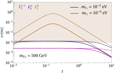
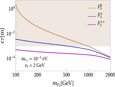
In the rest of this subsection we will assume $Y_{\Psi}=Y_{\overline{\Psi}}$. In this part of the parameter space, the more general neutrino fit of Cordero-Carrión et al. (2019a, b) essentially reduces to a Casas-Ibarra parametrization. Choosing again b.f.p. values for the neutrino data and ${\cal R}=1$, the decay length of the neutral, singly charged and doubly charged components of ${\bf 3}_{1}^{F}=(F_{3}^{0},F_{3}^{+},F_{3}^{++}$) are depicted in the left panel of Fig.7. The figure shows that the maximal decay length for $F^{+}$ can be of the order of $c\tau=1$ mm, while $F^{++}$ decays always with lengths smaller than mm. $F^{0}$, on the other hand, can have very large decay lengths. The different behaviour of the widths of these states is again due to the decays to pions, as discussed above.

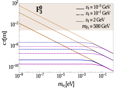
In the rest of this subsection, we will discuss only the decay lengths of the neutral components. In the right panel of Fig.7 we show the decay length of $F_{3}^{0}$ for different values of the scalar quadruplet vev $v_{\mathbf{4}}$. The solid, dashed and dotted lines correspond to the cases where $v_{\mathbf{4}}=10^{-3}$ GeV, $v_{\mathbf{4}}=10^{-1}$ GeV and $v_{\mathbf{4}}=2$ GeV respectively. For all the cases, we fixed the mass of the $F_{3}^{0}$, denoted as $m_{F_{3}}$, to 500 GeV. Orange, blue and magenta lines correspond again to the cases where the lightest of the three neutral triplets $F_{3_{i}}^{0}$ is the one associated with $m_{\nu_{i}}$, $i=1,2,3$. Larger values of the vev $v_{\bf 4}$ imply smaller Yukawas, for the same values of light neutrino masses, and thus larger lengths. From the figure, we can conclude that, for example, for a fixed value of $v_{\mathbf{4}}=10^{-3}$ GeV, the decay length is $c\tau\gtrsim 1$ mm as long as $m_{\nu_{1}}\lesssim 5\times 10^{-7}$ eV, while for a fixed value of $v_{\mathbf{4}}=2$ GeV, the decay length is $c\tau\gtrsim 1$ mm as long as $m_{\nu_{1}}\lesssim 5\times 10^{-4}$ eV. Recall, that there is an upper limit of roughly $v_{\bf 4}\raise 1.29167pt\hbox{$\;<$\kern-7.5pt\raise-4.73611pt\hbox{$\sim\;$}}3.5$ GeV, as discussed in section II.

III.3 $d=9$

In the $d=9$ model, introduced in section II, there are three different fermionic multiplets: $\mathbf{3_{1}^{F}}$, $\mathbf{4_{1/2}^{F}}$ and $\mathbf{5_{0}^{F}}$. The decay lengths of the lightest fermions then sensitively depends on which of these multiplets is the lightest. This is shown in fig. (8) in the left panel.

Figure 8: Left panel: Decay length for the neutral components of triplet, quadruplet and quintuplet fermion. Right panel: Decay length for the neutral, singly-charged and double-charged components of a quintuplet. For both panels, the lightest neutrino is fixed to $m_{\nu}=10^{-5}$ eV and the values of the Yukawas ${\overline{Y}}_{\bf 34}=Y_{\bf 45}=1$ and ${\overline{Y}}_{\bf 45}=Y_{\bf 34}=0$.

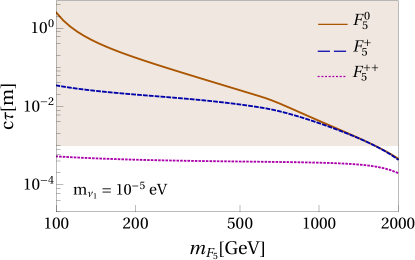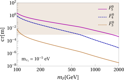
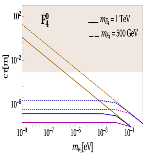
Fig. (8), left panel, shows $c\tau$ as a function of the mass of the fermion for a fixed choice of the lightest neutrino mass. Here, we have fixed the diagonal elements of the Yukawas ${\overline{Y}}_{\bf 34}=Y_{\bf 45}=1$ and ${\overline{Y}}_{\bf 45}=Y_{\bf 34}=0$. This choice of Yukawa couplings is motivated by the fact that to lowest order neutrino masses do not depend on ${\overline{Y}}_{\bf 45}$ and $Y_{\bf 34}=0$, see section II. We set either $M_{\bf 3}$ or $M_{\bf 4}$ or $M_{\bf 5}$ the smallest mass parameter, such that the lightest state is (correspondingly) either mostly a triplet, a quadruplet or a quintuplet fermion. While for a quintuplet (and partially also for a quadruplet) fermion sizeable lengths appear, triplet fermions have decay lengths two orders or more shorter than those found for the quintuplet.

This fact can be understood as follows. The decay width of the heavy fermions can be written roughly as:

$$\Gamma(F_{3,4,5}^{0})\propto|V_{3,4,5}|^{2}\frac{m_{F}^{3}}{m_{W}^{2}}.$$ (27)

From the structure of the neutral fermion mass matrix in this model, compare to eq. (15), one can estimate very approximately:

$$V_{3} \simeq m_{D}M_{\bf 3}^{-1}$$

$$V_{4} \simeq m_{D}M_{\bf 3}^{-1}m_{34}M_{\bf 4}^{-1}$$

$$V_{5} \simeq m_{D}M_{\bf 3}^{-1}m_{34}M_{\bf 4}^{-1}m_{45}M_{\bf 5}^{-1}$$ (28)

where $m_{D}\simeq\frac{v}{\sqrt{2}}Y_{\Psi}$, $m_{34}=\frac{v}{\sqrt{6}}{\overline{Y}}_{\bf 34}$ and $m_{45}=\frac{v}{2}Y_{\bf 45}$, respectively. Thus, one will find typically $V_{5}<V_{4}\ll V_{3}$, if the $M_{\bf i}$ are larger than the $m_{ij}$. Recall, that neutrino mass require at least some of these parameter ratios to be small, see eq. (16).

In the right panel of fig. (8), we show the decay lengths for the neutral, singly charged and doubly charged components of $\mathbf{5_{0}^{F}}$. The figure demonstrates that the largest lengths again are expected for the neutral component. The maximal allowed decay length of $F_{5}^{+}$ ($F_{5}^{++}$) is around $c\tau\simeq 1.8$ cm ($c\tau\simeq 0.4$ mm) for masses larger than 400 GeV. The reason is the same as discussed in the cases of seesaw type-III and the BNT model: The charged components of the multiplet are slightly heavier than the neutral one and, thus, can decay to the neutral state plus a a charged pion with a width that is numerically small, but not suppressed by the small neutrino mass.

Figure 9: Decay lengths for the neutral component of the triplet (left panel), quadruplet (central panel) and quintuplet (right panel) fermion. For the three cases, the dashed and continuous lines correspond to the choice of the lightest fermion mass of 500 GeV and 1 TeV respectively. Yukawas chosen as in fig. (8).

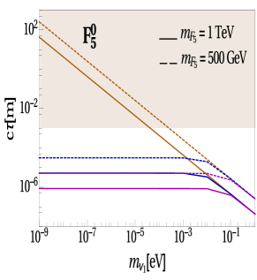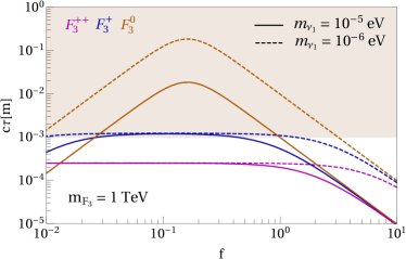
The decay lengths of the neutral components of $\mathbf{3_{1}^{F}}$, $\mathbf{4_{1/2}^{F}}$ and $\mathbf{5_{0}^{F}}$ are shown in Fig.9. For the three panels, the orange, blue and magenta lines again correspond to the cases where the lightest fermions is associated to the first, second and third neutrino mass eigenvalue, as obtained from a Cassa-Ibarra fit to neutrino data. For each case, the other free Yukawas of the model are fixed to 1, for simplicity.

As expected, the region in parameter space where measurable decay lengths occur are largest for fermions from the quintuplet, followed by quadruplet fermions, while the triplet fermions have unmeasurably short decay lengths practically in all acceptable parts of the parameter space. Note the change in scale in the plot for the triplets.

In summary, a systematic analysis of the fermionic decays from $d=5$ up to $d=9$ tree-level neutrino models allows us to conclude that for all models larger decay lengths are found for a smaller overall neutrino mass scale. In contrast larger masses of the fermions lead to smaller widths in all cases. We note that the charged components of the multiplets have in all cases a maximal value for their decay lengths, imposed by decays to the neutral fermion plus a charged pion. This decay is suppressed by a small mass splitting, but not by the small neutrino masses. We note that the maximal lengths for the charged components are different in seesaw type-III, BNT and the $d=9$ model. This might serve as a distinguishing feature for the different models.

IV Scalar decays

In this section we discuss the decays of the different scalars that appear in the neutrino tree-level mass models at dimensions $d=5,7$ and $d=11$, as introduced in section II. We will concentrate on the main decay modes only and on identifying the parameter region in which the decay lengths of the scalars are maximized.

As discussed in the introduction, various experimental searches by the LHC collaborations for type-II scalars (i.e. the case $d=5$) exist in the literature, see for example Aaboud et al. (2018); Collaboration (2017); Aaboud et al. (2019), to name the most recent ones. The scalars of the $d=7$ and $d=11$ models can be produced at the LHC in both, pair- and associated production. Since pair production cross sections at LHC scale, at large masses, proportional to the 4th power of the electric charge of the particle, one expects in general larger cross sections at the LHC, and thus better sensitivity to the scalars of these models than for seesaw type-II. However, so far no dedicated LHC searches for these states exist and, thus, there are no exact numbers on the lower limits on the masses of these particles. We will, very roughly, assume that all these scalars have masses in the range of [0.5,2] TeV, where the lower end of the range could most likely already be excluded with current data, if the final states of the scalar decays involve leptons.

IV.1 $d=5$

The simplest case we consider corresponds to the type-II seesaw model Schechter and Valle (1980); Mohapatra and Senjanovic (1981); Cheng and Li (1980) which has already been widely studied in the literature Chun et al. (2003); Fileviez Perez et al. (2008); Ferreira et al. (2019); Antusch et al. (2019); Du et al. (2019); Bhupal Dev and Zhang (2018); Dev et al. (2018); Cai et al. (2018); Bonilla et al. (2018); Reig et al. (2016); Mitra et al. (2017). In particular the authors of Refs. Du et al. (2019); Bhupal Dev and Zhang (2018) studied the parameter region in which the scalar mediators of the type-II seesaw model can be relatively long-lived. Since this case can be understood as the “proto-type” for the scalar decays in our other models, we briefly discuss seesaw type-II first.

As already mentioned, the type-II seesaw model adds a scalar SU(2) triplet $\Delta=(\Delta^{0},\Delta^{+},\Delta^{++})$ to the SM. We mention that one expects the decay length of the scalars to have similar values for different components of the triplet, especially for large masses. Note, that this assumes that the different members of the triplet have very similar masses, which is generally true for large values of $m_{\Delta}$. We will therefore discuss only the decays of $\Delta^{++}$.

The doubly charged scalar $\Delta^{++}$ has two decay modes: $\Delta^{++}\rightarrow W^{+}W^{+}$ and $\Delta^{++}\rightarrow l^{+}l^{+}$. These partial decay widths can be expressed as Chun et al. (2003); Fileviez Perez et al. (2008):

$$\Gamma(\Delta^{++}\rightarrow W^{+}W^{+})=\frac{\alpha_{2}}{32}\frac{v^{2}_{\Delta}m^{3}_{\Delta}}{v^{2}m^{2}_{W}}I_{2},\ \ \ \ \Gamma(\Delta^{++}\rightarrow l^{+}l^{+})=\frac{1}{16\pi}\frac{m_{\Delta}\sum_{i}m^{2}_{\nu_{i}}}{v^{2}_{\Delta}}$$ (29)

with

$$I_{2}=(1-4r_{W}+12r^{2}_{W})(1-4r_{W})^{1/2}\ \ ,\ \ r_{W}=(\frac{m_{W}}{m_{\Delta}})^{2}.$$ (30)

Here, summation over the lepton generations $\alpha=e,\mu,\tau$ is implicitly understood. The leptonic decay channel is proportional to the sum of the squares of the neutrino masses. This square has a minimum value of roughly $\sum_{i}m^{2}_{\nu_{i}}\raise 1.29167pt\hbox{$\;>$\kern-7.5pt\raise-4.73611pt\hbox{$\sim\;$}}(0.05\text{eV})^{2}$, corresponding to a normal hierarchy of neutrino masses with an atmospheric neutrino mass scale of $m_{\nu_{3}}\simeq\sqrt{\Delta m^{2}_{\rm Atm}}\simeq 0.05$ eV. Since $\Gamma(\Delta^{++}\rightarrow W^{+}W^{+})\propto v^{2}_{\Delta}$, while $\Gamma(\Delta^{++}\rightarrow l^{+}l^{+})\propto v^{-2}_{\Delta}$, there exists a value of $v_{\Delta}$ for which the total decay width is minimized. The corresponding maximum for the decay length is found for, in the limit $m_{\Delta}\gg m_{W}$:

$$(v_{\Delta})_{max}=\Big{(}\frac{2\sum_{i}m^{2}_{\nu_{i}}v^{2}m^{2}_{W}}{\alpha_{2}m_{\Delta}^{2}I_{2}}\Big{)}^{1/4}.$$ (31)

At $v_{\Delta}$ smaller than this value, the decays are dominated by leptonic final states, while for $v_{\Delta}$ larger than eq. (31) gauge boson final states dominate. Interestingly, the point in which the total decay width is minimized corresponds to equal branching ratios of $\Delta^{++}$ decaying into leptons and gauge bosons. For pair production $\Delta^{++}\Delta^{--}$ this corresponds to final states $(l^{+}l^{+}l^{-}l^{-}:l^{\pm}l^{\pm}W^{\mp}W^{\mp}:W^{+}W^{+}W^{-}W^{-})\simeq(1:2:1)$, thus maximizing the chances to see lepton number violation experimentally.

Figure 10: Decay length ($c\tau$) versus $v_{\Delta}$. Three different choices for $m_{\Delta}$, corresponding to $m_{\Delta}=200,500,1000$ GeV are shown. Dashed gray lines correspond to “partial inverse widths” $c\Gamma^{-1}(\Delta^{++}\rightarrow W^{+}W^{+})$ and $c\Gamma^{-1}(\Delta^{++}\rightarrow l^{+}l^{+})$ for $m_{\Delta}=200$ GeV. These lines are shown only for illustration. $\Delta^{++}\rightarrow W^{+}W^{+}$ and $\Delta^{++}\rightarrow l^{+}l^{+}$ indicate the parameter range, where the corresponding final state dominates the decay width.

This can be seen also in Fig. 10. As shown in this plot, for $m_{\Delta}=(1000,500,200)$ GeV there is maximum value of $c\tau$ as function $v_{\Delta}$. This maximum occurs at slightly smaller values than predicted by eq. (31), $v_{\Delta}\sim(1,2,3)\times 10^{-4}$ GeV, due to phase space effects. The dashed gray lines in the background indicate the different partial widths for the case of $m_{\Delta}=200$ GeV. These lines are for illustration purposes only, to demonstrate where lepton or gauge boson final states are dominant. The heavier (lighter) $\Delta^{++}$ the smaller (larger) the maximum value of $c\tau$ becomes. Fig. 10 also shows a gray band which correspond $c\tau>1$ mm. As we can see in this figure, given current neutrino data, the scalar mediators of the seesaw type-II always have $c\tau<<1$ mm for $m_{\Delta}>200$ GeV. Thus, a doubly charged scalar with $m>200$ GeV, decaying with a visible decay length can not give the correct explanation for the observed neutrino masses, as expected from seesaw type-II.

IV.2 $d=7$

We now turn to the case of the BNT model Babu et al. (2009). The scalar quadruplet with hypercharge $3/2$, can be written in components as ${\bf 4^{S}_{3/2}}=(S^{3+}_{4},S^{2+}_{4},S^{+}_{4},S^{0}_{4})$. Consider first the triply charged scalar $S_{4}^{3+}$. It has two principal decay modes: $S^{3+}_{4}\rightarrow W^{+}W^{+}W^{+}$ and $S^{3+}_{4}\rightarrow W^{+}l^{+}l^{+}$, where again we have suppressed flavour indices for the leptons. Pair production of $S_{4}^{3+}$ can lead therefore to final states with up to 6 $W$s or 4 leptons plus 2 $W$. Of particular theoretical interest are the LNV final states of $l^{+}l^{+}$+8 jets (from hadronically decaying $W$s).

In the limit where the mass of $S^{3+}_{4}$ is large, $m_{4}\gg m_{W}$, one can find an approximate expression for the partial decay widths of $S^{3+}_{4}$:

$$\Gamma(S^{3+}\rightarrow W^{+}W^{+}W^{+})\sim\frac{3g^{6}}{2048\pi^{3}}\frac{v^{2}_{4}m^{5}_{4}}{m^{6}_{W}},\hskip 42.67912pt\Gamma(S^{3+}\rightarrow W^{+}l^{+}l^{+})\sim\frac{g^{2}}{3072\pi^{3}}\frac{m^{3}_{4}\sum_{i}m^{2}_{\nu_{i}}}{v^{2}_{4}m^{2}_{W}}.$$ (32)

Note that we have used here the phase space for massless final state particles, thus eq. (32) approaches the numerical result, see below, only for $m_{4}\gg m_{W}$.

Compared to the case of the seesaw type-II, discussed previously, one notes that the partial widths are suppressed by phase space factors for the three particle final state, but enhanced by different additional factors $(m_{4}/m_{W})^{2}$. The latter is due to the fact that in the limit of large scalar masses the decays to the longitudinal component of the $W$ dominates the total decay width.

Most important, however, is that the decay width $\Gamma(S^{3+}\rightarrow W^{+}W^{+}W^{+})$ is proportional to $v_{4}^{2}$, while $\Gamma(S^{3+}\rightarrow W^{+}l^{+}l^{+})\propto v_{4}^{-2}$, similar to the case of the seesaw type-II. Thus, using Eq. (32) we can estimate a value $(v_{4})_{max}$, which maximizes the decay length, as:

$$(v_{4})_{max}\sim\frac{(\sum_{i}m^{2}_{\nu_{i}})^{1/4}m_{W}}{\sqrt{3}g\sqrt{m_{4}}}$$ (33)

Roughly, this gives $(v_{4})_{max}\sim 2\times 10^{-5}$ GeV for $\sum_{i}m^{2}_{\nu_{i}}=(0.05)^{2}$ eV² and the example $m_{4}\simeq 800$ GeV.

Figure 11: Decay lenghth ($c\tau$) versus $v_{4}$. Solid, dashed and dotted lines correspond to $m_{4}=500,600,800$ GeV respectively. Dashed gray lines correspond to $c\Gamma^{-1}(S_{4}^{3+}\rightarrow W^{+}W^{+}W^{+})$ and $c\Gamma^{-1}(S_{4}^{+3}\rightarrow W^{+}l^{+}l^{+})$ for $m_{4}=500$ GeV.

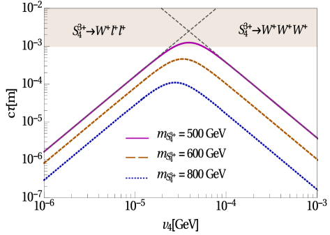
With the SARAH generated model files for the BNT model, we used MadGraph Alwall et al. (2007, 2011, 2014) for a numerical calculation of the partial widths of $S^{3+}_{4}$. The results are shown in fig. (11). The figure shows $c\tau$ for $S^{3+}_{4}$ for three values of $m_{4}$, $m_{4}=500,600,800$ GeV, as a function of $v_{4}$. As before, the grey area indicates $c\tau>1$ mm. As discussed above, there is a value of $v_{4}$ for which the decay length has a maximum, $(v_{4})_{max}\sim(10^{-5}-10^{-4})$ GeV. Comparison of the numerical values of $(v_{4})_{max}$ with those predicted by eq. (33), show that the latter underestimates the true value for small values of $m_{4}$, but is quite accurate for, say, $m_{4}\raise 1.29167pt\hbox{$\;>$\kern-7.5pt\raise-4.73611pt\hbox{$\sim\;$}}1$ TeV. The figure also shows that the total decay lengths, $c\tau$, should be shorter than $\sim 1$ mm for masses larger than roughly $500$ GeV. Note that $c\tau$ does not include possible boosts from production, such that visible decay lengths may occur experimentally still for masses slightly larger than $500$ GeV.

We now turn to a brief discussion of the decays of $S^{2+}_{4}$. Similar to the case of the $\Delta^{++}$ of the seesaw type-II, the main final states for the decays of the $S^{2+}_{4}$ are $W^{+}W^{+}$ and $l^{+}l^{+}$. In the limit of large masses, $m_{4}\gg m_{W}$ we can estimate the ratio of the total widths as:

$$\frac{\Gamma^{\rm tot}(S^{2+}_{4})}{\Gamma^{\rm tot}(S^{3+}_{4})}\sim\frac{1}{g^{2}}\frac{f(3)}{f(2)}\frac{m_{W}^{2}}{m_{4}^{2}}\simeq\frac{32\pi^{2}}{g^{2}}\frac{m_{W}^{2}}{m_{4}^{2}}$$ (34)

Here $f(n)=4(4\pi)^{2n-3}(n-1)!(n-2)!$ takes care of the phase space volume available to the decay products of $n$ massless particles, see ref. Fonseca et al. (2018). From eq. (34) one estimates that $S^{2+}$ should decay with widths roughly a factor $\sim 8$ ($\sim 5$) larger than $S^{3+}$ for masses order $m_{4}=800$ GeV (1 TeV). Comparison with the numerical results in fig. 11 shows that one can not expect to have a visible decay length for $S^{2+}$, similar to what is shown in fig. 10 for the $\Delta^{++}$ of the seesaw type-II.

IV.3 $d=11$

The last case we dissus are the scalars of the $d=11$ tree-level neutrino mass model, defined in section II. This model introduces three different scalars: ${\bf 5}^{S}_{2}$, ${\bf 5}^{S}_{1}$ and ${\bf 3}^{S}_{0}$ as can be seen in Fig. 4 (to the right). Decay lengths of the scalars in this model depend on their mass hierarchy. In our discussion we will assume the lightest heavy particle is ${\bf 5}^{S}_{2}$, i.e. $m_{5_{2}}<m_{5_{1}},m_{3}$. This is motivated by the observation that the decay widths of the scalars to final states with gauge bosons will scale with the square of the vev of the neutral component of the corresponding scalar multiplet, similar to the situation in the other models discussed above. As eqs (19)-(21) show, from the tadpole equations one expects that the vev of ${\bf 5}^{S}_{2}$, $v_{52}$, is numerically the smallest of the three vevs. Also, ${\bf 5}^{S}_{2}=(S^{+4}_{5},S^{+3}_{5},S^{+2}_{5},S^{+}_{5},S^{0}_{5})$ contains a quadruply charged scalar, which can be expected to have the smallest decay width of all the scalars in the model, due to the additional phase space suppressions.

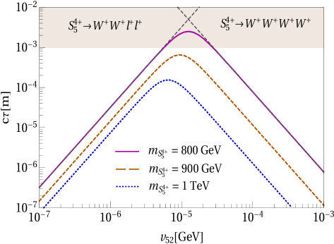
Fig. 12 shows $c\tau$ for $S^{+4}_{5}$ versus $v_{52}$ for three different values of $m_{5_{2}}$, $m_{5_{2}}=0.8,0.9$ and $1$ TeV. The two dominant decay modes here are $S_{5}^{4+}\rightarrow W^{+}W^{+}W^{+}W^{+}$ and $S_{5}^{4+}\rightarrow W^{+}W^{+}l^{+}l^{+}$. Again, the numerical calculation of the widths were done using MadGraph Alwall et al. (2007, 2011, 2014), based on our private version of the SARAH generated model files for the $d=11$ model.

As one can see in this figure there is a maximum around $v_{52}\sim 10^{-5}$ GeV, slightly different for different values of $m_{5_{2}}$. The explanation for this feature is the same as in the seesaw type-II and the BNT model, discussed previously. The leptonic decay mode $S_{5}^{4+}\rightarrow W^{+}W^{+}l^{+}l^{+}$ is proportional to $1/v_{52}^{2}$ while $S_{5}^{4+}\rightarrow W^{+}W^{+}W^{+}W^{+}$ scales as $v^{2}_{52}$. Therefore, there will be a maximum value $(v_{52})_{max}$ for which if $v_{52}<<(v_{52})_{max}$ the leptonic mode will dominate while if $v_{52}>>(v_{52})_{max}$ the decay mode $W^{+}W^{+}W^{+}W^{+}$ will be the dominant contribution of $c\tau$.

As fig. 12 shows, there exists a region in parameter space, for which $S_{5}^{4+}$ can decay with a visible decay length. Visible decay lengths are possible up to masses very roughly in the range of ($800-900$) GeV. The explanation for these larger masses for the case of $S_{5}^{4+}$ compared to the $S_{4}^{3+}$ of the BNT model is the large suppression from the 4-body phase space. This suppression is only partially compensated by an additional factor of $\frac{m_{5_{2}}^{2}}{m_{W}^{2}}$ in the decay width for the additional $W$ boson in the final state.

We close the discussion of the $d=11$ scalars by mentioning that all other scalars in the model should have a smaller decay length than $S_{5}^{4+}$. The explanation for this is essentially smaller phase space suppression for the decay widths of the other scalars, very similar to the case of the BNT model discussed previously.

Figure 12: Decay lenghth ($c\tau$) versus $v_{52}$. Solid, dashed and dotted lines correspond to $m_{5_{2}}=800,900,1000$ GeV respectively.

In summary, from the analysis of the scalar decays in tree-level neutrino mass models at $d=5,7,11$ we can conclude that in all cases there is an upper limit of the decay length, different from the situation found for (neutral) fermions. For the scalars of the $d=7$ and $d=11$ models this upper limit is of the order of a few millimeters, and thus still in an observable range, while for the type-II seesaw one does not expect to see a finite decay length experimentally. In all cases this upper limit is reached in a region of parameter space in which leptonic and gauge boson final states have similar branching ratios.

V Conclusions

We have studied LHC phenomenology of different neutrino mass models. All our models generate neutrino masses at tree-level. They range from the simplest $d=5$ seesaws to $d=11$ models. Our main focus was to study the decays of the heavy seesaw mediators. We concentrated on masses below roughly 2 TeV, such that the heavy particles can be produced at the high-luminosity LHC. We calculated the decay widths for the fermions and scalars, that appear in the different models. Our results depend on the unknown spectrum of mediators, i.e. we have to distinguish two scenarios: (i) the exotic fermions are the lighter of the mediators and (ii) scalars are lighter than the exotic fermions.

For case (i), fermions being the lighter (heavy) particles, we find that their mixing with standard model particles is suppressed by the light neutrino masses. Since there is no experimental lower limit on the lightest neutrino mass, this mixing can be very small, leading to very slow decays. Very large decay lengths for neutral fermions are then possible, even for fermions with masses order ${\cal O}$(TeV). In general, the fermions from models with $d>5$ tend to have smaller decay lengths than those found for the fermions in $d=5$ models.

The situation is different for scalars. In high-dimensional models, large scalar multiplets need to be introduced. Due to large phase space suppression factors, the multiply charged scalars in these models tend to have very small widths. As we have discussed scalars in these models can decay either to pure gauge boson final states or to final states with pairs of leptons (plus additional gauge bosons). Since these two final states depend differently on the vacuum expectation values of the scalars, there is always an upper limit on the maximally allowed decay length. The numerical value of this maximal decay length depends on the electric charge of the scalar under consideration, but can not be larger than typically a few millimeters. Interestingly the maximal decay length always appears in a parameter region in which it should be possible to observe lepton number violating final states.

Finally, as we have mentioned before, with the exception of the well-known seesaw type-II, no LHC searches exist for any of the exotic scalars we considered in this paper. Since these scalars can have very high-multiplicity final states, we expect backgrounds to be low at the LHC. This, combined with the large production cross sections for multiply charged particles, makes LHC searches for these exotic scalars very promising, in principle.

Acknowledgements

M. H. acknowledges funding by Spanish grants FPA2017-90566-REDC (Red Consolider MultiDark), FPA2017-85216-P and SEV-2014-0398 (AEI/FEDER, UE), as well as PROMETEO/2018/165 (Generalitat Valenciana). C.A. is supported by Chile grant Fondecyt No. 11180722 and CONICYT PIA/Basal FB0821. J. C. H. is supported by Chile grant Fondecyt No. 1161463.

References

- Alimena et al. (2019) J. Alimena et al. (2019), eprint 1903.04497.
- Chou et al. (2017) J. P. Chou, D. Curtin, and H. J. Lubatti, Phys. Lett. B767, 29 (2017), eprint 1606.06298.
- Curtin et al. (2018) D. Curtin et al. (2018), eprint 1806.07396.
- Gligorov et al. (2017) V. V. Gligorov, S. Knapen, M. Papucci, and D. J. Robinson (2017), eprint 1708.09395.
- Feng et al. (2017) J. Feng, I. Galon, F. Kling, and S. Trojanowski (2017), eprint 1708.09389.
- Alekhin et al. (2016) S. Alekhin et al., Rept. Prog. Phys. 79, 124201 (2016), eprint 1504.04855.
- Pinfold et al. (2009) J. Pinfold et al. (MoEDAL) (2009).
- Minkowski (1977) P. Minkowski, Phys.Lett. B67, 421 (1977).
- Yanagida (1979) T. Yanagida, Conf.Proc. C7902131, 95 (1979).
- Mohapatra and Senjanovic (1980) R. N. Mohapatra and G. Senjanovic, Phys. Rev. Lett. 44, 912 (1980).
- Helo et al. (2014) J. C. Helo, M. Hirsch, and S. Kovalenko, Phys. Rev. D89, 073005 (2014), [Erratum: Phys. Rev.D93,no.9,099902(2016)], eprint 1312.2900.
- Deppisch et al. (2018) F. F. Deppisch, W. Liu, and M. Mitra (2018), eprint 1804.04075.
- Helo et al. (2018) J. C. Helo, M. Hirsch, and Z. S. Wang, JHEP 07, 056 (2018), eprint 1803.02212.
- Nemevšek et al. (2018) M. Nemevšek, F. Nesti, and G. Popara, Phys. Rev. D97, 115018 (2018), eprint 1801.05813.
- Lara et al. (2018) I. Lara, D. E. López-Fogliani, C. Muñoz, N. Nagata, H. Otono, and R. Ruiz De Austri (2018), eprint 1804.00067.
- Dev et al. (2017) P. S. B. Dev, R. N. Mohapatra, and Y. Zhang, Nucl. Phys. B923, 179 (2017), eprint 1703.02471.
- Cottin et al. (2018) G. Cottin, J. C. Helo, and M. Hirsch, Phys. Rev. D98, 035012 (2018), eprint 1806.05191.
- Cottin et al. (2019) G. Cottin, J. C. Helo, M. Hirsch, and D. Silva (2019), eprint 1902.05673.
- Dercks et al. (2019) D. Dercks, H. K. Dreiner, M. Hirsch, and Z. S. Wang, Phys. Rev. D99, 055020 (2019), eprint 1811.01995.
- Casas and Ibarra (2001) J. Casas and A. Ibarra, Nucl.Phys. B618, 171 (2001), eprint hep-ph/0103065.
- Aghanim et al. (2018) N. Aghanim et al. (Planck) (2018), eprint 1807.06209.
- Gando et al. (2016) A. Gando et al. (KamLAND-Zen), Phys. Rev. Lett. 117, 082503 (2016), [Addendum: Phys. Rev. Lett.117,no.10,109903(2016)], eprint 1605.02889.
- Agostini et al. (2018) M. Agostini et al. (GERDA), Phys. Rev. Lett. 120, 132503 (2018), eprint 1803.11100.
- Atre et al. (2009) A. Atre, T. Han, S. Pascoli, and B. Zhang, JHEP 05, 030 (2009), eprint 0901.3589.
- Bondarenko et al. (2018) K. Bondarenko, A. Boyarsky, D. Gorbunov, and O. Ruchayskiy, JHEP 11, 032 (2018), eprint 1805.08567.
- Mohapatra and Valle (1986) R. Mohapatra and J. Valle, Phys. Rev. D34, 1642 (1986).
- Foot et al. (1989) R. Foot, H. Lew, X. He, and G. C. Joshi, Z.Phys. C44, 441 (1989).
- Franceschini et al. (2008) R. Franceschini, T. Hambye, and A. Strumia, Phys. Rev. D78, 033002 (2008), eprint 0805.1613.
- Jana et al. (2018) S. Jana, N. Okada, and D. Raut, Phys. Rev. D98, 035023 (2018), eprint 1804.06828.
- Deppisch et al. (2019) F. F. Deppisch, S. Kulkarni, and W. Liu (2019), eprint 1905.11889.
- Weinberg (1979) S. Weinberg, Phys. Rev. Lett. 43, 1566 (1979).
- Ma (1998) E. Ma, Phys.Rev.Lett. 81, 1171 (1998), eprint hep-ph/9805219.
- Schechter and Valle (1980) J. Schechter and J. Valle, Phys. Rev. D22, 2227 (1980).
- Bonnet et al. (2009) F. Bonnet, D. Hernandez, T. Ota, and W. Winter, JHEP 10, 076 (2009), eprint 0907.3143.
- Babu et al. (2009) K. S. Babu, S. Nandi, and Z. Tavartkiladze, Phys. Rev. D80, 071702 (2009), eprint 0905.2710.
- Aristizabal Sierra et al. (2015) D. Aristizabal Sierra, A. Degee, L. Dorame, and M. Hirsch, JHEP 03, 040 (2015), eprint 1411.7038.
- Cepedello et al. (2018) R. Cepedello, R. M. Fonseca, and M. Hirsch, JHEP 10, 197 (2018), eprint 1807.00629.
- Anamiati et al. (2018) G. Anamiati, O. Castillo-Felisola, R. M. Fonseca, J. C. Helo, and M. Hirsch, JHEP 12, 066 (2018), eprint 1806.07264.
- Tanabashi et al. (2018) M. Tanabashi et al. (Particle Data Group), Phys. Rev. D98, 030001 (2018).
- Aaboud et al. (2018) M. Aaboud et al. (ATLAS), Eur. Phys. J. C78, 199 (2018), eprint 1710.09748.
- Collaboration (2017) C. Collaboration (CMS) (2017).
- Aaboud et al. (2019) M. Aaboud et al. (ATLAS), Eur. Phys. J. C79, 58 (2019), eprint 1808.01899.
- Sirunyan et al. (2017) A. M. Sirunyan et al. (CMS), Phys. Rev. Lett. 119, 221802 (2017), eprint 1708.07962.
- Ghosh et al. (2018a) K. Ghosh, S. Jana, and S. Nandi, JHEP 03, 180 (2018a), eprint 1705.01121.
- Ghosh et al. (2018b) T. Ghosh, S. Jana, and S. Nandi, Phys. Rev. D97, 115037 (2018b), eprint 1802.09251.
- Akhmedov et al. (1996a) E. K. Akhmedov, M. Lindner, E. Schnapka, and J. Valle, Phys.Lett. B368, 270 (1996a), eprint hep-ph/9507275.
- Akhmedov et al. (1996b) E. K. Akhmedov, M. Lindner, E. Schnapka, and J. Valle, Phys.Rev. D53, 2752 (1996b), eprint hep-ph/9509255.
- Staub (2013) F. Staub, Comput.Phys.Commun. 184, pp. 1792 (2013), eprint 1207.0906.
- Staub (2014) F. Staub, Comput.Phys.Commun. 185, 1773 (2014), eprint 1309.7223.
- Porod (2003) W. Porod, Comput.Phys.Commun. 153, 275 (2003), eprint hep-ph/0301101.
- Porod and Staub (2012) W. Porod and F. Staub, Comput.Phys.Commun. 183, 2458 (2012), eprint 1104.1573.
- Alwall et al. (2007) J. Alwall, P. Demin, S. de Visscher, R. Frederix, M. Herquet, et al., JHEP 0709, 028 (2007), eprint 0706.2334.
- Alwall et al. (2011) J. Alwall, M. Herquet, F. Maltoni, O. Mattelaer, and T. Stelzer, JHEP 1106, 128 (2011), eprint 1106.0522.
- Alwall et al. (2014) J. Alwall, R. Frederix, S. Frixione, V. Hirschi, F. Maltoni, et al., JHEP 1407, 079 (2014), eprint 1405.0301.
- Staub et al. (2012) F. Staub, T. Ohl, W. Porod, and C. Speckner, Comput. Phys. Commun. 183, 2165 (2012), eprint 1109.5147.
- Anamiati et al. (2016) G. Anamiati, M. Hirsch, and E. Nardi, JHEP 10, 010 (2016), eprint 1607.05641.
- Cordero-Carrión et al. (2019a) I. Cordero-Carrión, M. Hirsch, and A. Vicente, Phys. Rev. D99, 075019 (2019a), eprint 1812.03896.
- Cordero-Carrión et al. (2019b) I. Cordero-Carrión, M. Hirsch, and A. Vicente, in 6th Symposium on Prospects in the Physics of Discrete Symmetries (DISCRETE 2018) Vienna, Austria, November 26-30, 2018 (2019b), eprint 1903.03330.
- Mohapatra and Senjanovic (1981) R. N. Mohapatra and G. Senjanovic, Phys. Rev. D23, 165 (1981).
- Cheng and Li (1980) T. P. Cheng and L.-F. Li, Phys. Rev. D22, 2860 (1980).
- Chun et al. (2003) E. J. Chun, K. Y. Lee, and S. C. Park, Phys. Lett. B566, 142 (2003), eprint hep-ph/0304069.
- Fileviez Perez et al. (2008) P. Fileviez Perez, T. Han, G.-Y. Huang, T. Li, and K. Wang, Phys. Rev. D78, 071301 (2008), eprint 0803.3450.
- Ferreira et al. (2019) M. M. Ferreira, T. B. de Melo, S. Kovalenko, P. R. D. Pinheiro, and F. S. Queiroz (2019), eprint 1903.07634.
- Antusch et al. (2019) S. Antusch, O. Fischer, A. Hammad, and C. Scherb, JHEP 02, 157 (2019), eprint 1811.03476.
- Du et al. (2019) Y. Du, A. Dunbrack, M. J. Ramsey-Musolf, and J.-H. Yu, JHEP 01, 101 (2019), eprint 1810.09450.
- Bhupal Dev and Zhang (2018) P. S. Bhupal Dev and Y. Zhang, JHEP 10, 199 (2018), eprint 1808.00943.
- Dev et al. (2018) P. S. B. Dev, M. J. Ramsey-Musolf, and Y. Zhang, Phys. Rev. D98, 055013 (2018), eprint 1806.08499.
- Cai et al. (2018) Y. Cai, T. Han, T. Li, and R. Ruiz, Front.in Phys. 6, 40 (2018), eprint 1711.02180.
- Bonilla et al. (2018) C. Bonilla, J. M. Lamprea, E. Peinado, and J. W. F. Valle, Phys. Lett. B779, 257 (2018), eprint 1710.06498.
- Reig et al. (2016) M. Reig, J. W. F. Valle, and C. A. Vaquera-Araujo, Phys. Rev. D94, 033012 (2016), eprint 1606.08499.
- Mitra et al. (2017) M. Mitra, S. Niyogi, and M. Spannowsky, Phys. Rev. D95, 035042 (2017), eprint 1611.09594.
- Fonseca et al. (2018) R. M. Fonseca, M. Hirsch, and R. Srivastava, Phys. Rev. D97, 075026 (2018), eprint 1802.04814.