Compositional Abstraction-based Synthesis of General MDPs via Approximate Probabilistic Relations

Abstract.

We propose a compositional approach for constructing abstractions of general Markov decision processes using approximate probabilistic relations. The abstraction framework is based on the notion of $\delta$-lifted relations, using which one can quantify the distance in probability between the interconnected gMDPs and that of their abstractions. This new approximate relation unifies compositionality results in the literature by incorporating the dependencies between state transitions explicitly and by allowing abstract models to have either finite or infinite state spaces. Accordingly, one can leverage the proposed results to perform analysis and synthesis over abstract models, and then carry the results over concrete ones. To this end, we first propose our compositionality results using the new approximate probabilistic relation which is based on lifting. We then focus on a class of stochastic nonlinear dynamical systems and construct their abstractions using both model order reduction and space discretization in a unified framework. We provide conditions for simultaneous existence of relations incorporating the structure of the network. Finally, we demonstrate the effectiveness of the proposed results by considering a network of four nonlinear dynamical subsystems (together 12 dimensions) and constructing finite abstractions from their reduced-order versions (together 4 dimensions) in a unified compositional framework. We benchmark our results against the compositional abstraction techniques that construct both infinite abstractions (reduced-order models) and finite MDPs in two consecutive steps. We show that our approach is much less conservative than the ones available in the literature.

1. Introduction

Motivations. Control systems with stochastic uncertainty can be modeled as Markov decision processes (MDPs) over general state spaces. Synthesizing policies for satisfying complex temporal logic properties over MDPs evolving on uncountable state spaces is inherently a challenging task due to the computational complexity. Since closed-form characterization of such policies is not available in general, a suitable approach is to approximate these models by simpler ones possibly with finite or lower dimensional state spaces. A crucial step is to provide formal guarantees during this approximation phase, such that the analysis or synthesis on the simpler model can be refined back over the original one. In other words, one can first abstract the original model by a simpler one, and then carry the results from the simpler model to the concrete one using an interface map, by providing quantified errors on the approximation.

Related literature. Similarity relations over finite-state stochastic systems have been studied, either via exact notions of probabilistic (bi)simulation relations [LS91], [SL95] or approximate versions [DLT08], [DAK12]. Similarity relations for models with general, uncountable state spaces have also been proposed in the literature. These relations either depend on stability requirements on model outputs via martingale theory or contractivity analysis [JP09], [ZMEM⁺14] or enforce structural abstractions of a model [DGJP04] by exploiting continuity conditions on its probability laws [Aba13], [AKNP14]. These similarity relations are then used to relate the probabilistic behavior of a concrete model to that of its abstraction. There have been also several results on the construction of (in)finite abstractions for stochastic systems. Construction of finite abstractions for formal verification and synthesis is presented in [APLS08]. Extension of such techniques to automata-based controller synthesis and infinite horizon properties, and improvement of the construction algorithms in terms of scalability are proposed in [KSL13], [TA11], and [SA13], respectively.

In order to make the techniques applicable to networks of interacting systems, compositional abstraction and policy synthesis are studied in the literature. Compositional construction of finite abstractions using dynamic Bayesian networks is discussed in [SAM15]. Compositional construction of infinite abstractions (reduced-order models) is proposed in [LSMZ17, LSZ19a] using small-gain type conditions and dissipativity-type properties of subsystems and their abstractions, respectively. Compositional construction of finite abstractions is studied in [LSZ18a, LSZ18b]. Compositional modeling and analysis for the safety verification of stochastic hybrid systems are investigated in [HHHK13] in which random behaviour occurs only over the discrete components – this limits their applicability to systems with continuous probabilistic evolutions. Compositional modeling of stochastic hybrid systems is discussed in [Sv06] using communicating piecewise deterministic Markov processes that are connected through a composition operator. Recently, compositional synthesis of large-scale stochastic systems using a relaxed dissipativity approach is proposed in [LSZ19b].

Our Contributions. In our proposed framework, we consider the class of general Markov decisions processes (gMDPs), which evolves over continuous or uncountable state spaces, equipped with an output space and an output map. We encode interaction between gMDPs via internal inputs, as opposed to external inputs which are used for applying the synthesized policies enforcing some complex temporal logic properties. We provide conditions under which the proposed similarity relations between individual gMDPs can be extended to relations between their respective interconnections. These conditions enable compositional quantification of the distance in probability between the interconnected gMDPs and that of their abstractions. The proposed notion has the advantage of encoding prior knowledge on dependencies between uncertainties of the two models. Our compositional scheme allows constructing both infinite and finite abstractions in a unified framework. We benchmark our results against the compositional abstraction techniques of [LSZ18b, LSZ19a] which are based on dissipativity-type reasoning and provide a compositional methodology for constructing both infinite abstractions (reduced-order models) and finite MDPs in two consecutive steps. We show that our approach is much less conservative than the ones proposed in [LSZ18b, LSZ19a].

Recent Works. Similarities between two gMDPs have been recently studied in [HSA17] using a notion of $\delta$-lifted relation, but only for single gMDPs. The result is generalized in [HSA18] to a larger class of temporal properties and in [HS18] to synthesize policies for robust satisfaction of specifications. One of the main contributions of this paper is to extend this notion such that it can be applied to networks of gMDPs. This extension is inspired by the notion of disturbance bisimulation relation proposed in [MSSM16]. In particular, we extend the notion of $\delta$-lifted relation for networks of gMDPs and show that under specific conditions systems can be composed while preserving the relation. This type of relations enables us to provide the probabilistic closeness guarantee between two interconnected gMDPs (cf. Theorem 3.5). Furthermore, we provide an approach for the construction of finite MDPs in a unified framework for a class of stochastic nonlinear dynamical systems, considered as gMDPs, whereas the construction scheme in [HSA17] only handles the class of linear systems.

Organization. The rest of the paper is organized as follows. Section 2 defines the class of general Markov decision processes with internal inputs and output maps. Section 3 presents first the notion of $\delta$-lifted relations over probability spaces and then the notion of lifting for gMDPs. Section 4 provides compositional conditions for having the similarity relation between networks of gMDPs based on relations between their individual components. Section 5 provides details of constructing finite abstractions for a network of stochastic nonlinear control systems, which is based on both model order reduction and space discretization in a unified framework, together with the similarity relations. Finally, Section 6 demonstrates the effectiveness of our approach on a numerical case study.

2. General Markov Decision Processes

2.1. Preliminaries and Notations

In this paper, we work on Borel measurable spaces, i.e., $(X,\mathcal{B}(X))$, where $\mathcal{B}(X)$ is the Borel sigma algebra on $X$, and restrict ourselves to Polish spaces (i.e., separable and completely metrizable spaces). Given the measurable space $(X,\mathcal{B}(X))$, a probability measure $\mathbb{P}$ defines the probability space $(X,\mathcal{B}(X),\mathbb{P})$. We denote the set of all probability measures on $(X,\mathcal{B}(X))$ as $\mathcal{P}(X,\mathcal{B}(X))$. A map $f:S\rightarrow Y$ is measurable whenever it is Borel measurable.

The sets of nonnegative and positive integers, and real numbers are denoted by $\mathbb{N}:=\{0,1,2,\ldots\}$, $\mathbb{N}_{\geq 1}:=\{1,2,3,\ldots\}$, and $\mathbb{R}$, respectively. For column vectors $x_{i}\in\mathbb{R}^{n_{i}}$, $n_{i}\in\mathbb{N}_{\geq 1}$, and $i\in\{1,\ldots,N\}$, we denote by $x=[x_{1};\ldots;x_{N}]$ the corresponding column vector of dimension $\sum_{i}n_{i}$. Given a vector $x\in\mathbb{R}^{n}$, $\|x\|$ denotes the Euclidean norm of $x$. The identity and zero matrices in $\mathbb{R}^{n\times{n}}$ are denoted by $\mathds{I}_{n}$ and $\mathbf{0}_{n\times n}$, respectively. The symbols $\mathbf{0}_{n}$ and $\mathds{1}_{n}$ denote the column vector in $\mathbb{R}^{n}$ with all elements equal to zero and one, respectively. A diagonal matrix in $\mathbb{R}^{N\times{N}}$ with diagonal entries $a_{1},\ldots,a_{N}$ starting from the upper left corner is denoted by $\mathsf{diag}(a_{1},\ldots,a_{N})$. Given functions $f_{i}:X_{i}\rightarrow Y_{i}$, for any $i\in\{1,\ldots,N\}$, their Cartesian product $\prod_{i=1}^{N}f_{i}:\prod_{i=1}^{N}X_{i}\rightarrow\prod_{i=1}^{N}Y_{i}$ is defined as $(\prod_{i=1}^{N}f_{i})(x_{1},\ldots,x_{N})=[f_{1}(x_{1});\ldots;f_{N}(x_{N})]$. Given sets $X$ and $Y$, a relation $\mathscr{R}\subseteq X\times Y$ is a subset of the Cartesian product $X\times Y$ that relates $x\in X$ with $y\in Y$ if $(x,y)\in\mathscr{R}$, which is equivalently denoted by $x\mathscr{R}y$.

2.2. General Markov Decision Processes

In our framework, we consider the class of general Markov decision processes (gMDPs) that evolves over continuous or uncountable state spaces. This class of models generalizes the usual notion of MDP [BKL08] by including internal inputs that are employed for composition  [LSZ18b], and by adding an output space over which properties of interest are defined [HSA17].

Definition 2.1.

A general Markov decision process (gMDP) is a tuple

$$\Sigma=(X,W,U,\pi,T,Y,h)$$ (2.1)

where

• $X\subseteq\mathbb{R}^{n}$ is a Borel space as the state space of the system. We denote by $(X,\mathcal{B}(X))$ the measurable space with $\mathcal{B}(X)$ being the Borel sigma-algebra on the state space;

• $W\subseteq\mathbb{R}^{p}$ is a Borel space as the internal input space of the system;

• $U\subseteq\mathbb{R}^{m}$ is a Borel space as the external input space of the system;

• $\pi=\mathcal{B}(X)\rightarrow[0,1]$ is the initial probability distribution;

• $T:\mathcal{B}(X)\times X\times W\times U\rightarrow[0,1]$ is a conditional stochastic kernel that assigns to any $x\in X$, $w\in W$, and $\nu\in U$, a probability measure $T(\cdot|x,w,\nu)$ on the measurable space $(X,\mathcal{B}(X))$. This stochastic kernel specifies probabilities over executions $\{x(k),k\in\mathbb{N}\}$ of the gMDP such that for any set $\mathcal{A}\in\mathcal{B}(X)$ and any $k\in\mathbb{N}$,

  $$\mathbb{P}(x(k+1)\in\mathcal{A}\,\Big{|}\, x(k),w(k),\nu(k))=\int_{\mathcal{A}}T(dx(k+1)|x(k),w(k),\nu(k)).$$

• $Y\subseteq\mathbb{R}^{q}$ is a Borel space as the output space of the system;

• $h:X\rightarrow Y$ is a measurable function that maps a state $x\in X$ to its output $y=h(x)$.

Remark 2.2.

In this work, we are interested in networks of gMDPs that are obtained from composing gMDPs having both internal and external inputs and are synchronized through their internal inputs. The resulting interconnected gMDP will have only external input and will be denoted by the tuple $\Sigma=(X,U,\pi,T,Y,h)$ with stochastic kernel $T:\mathcal{B}(X)\times X\times U\rightarrow[0,1]$.

Evolution of the state of a gMDP $\Sigma$, can be alternatively described by

$$\Sigma:\left\{\begin{array}[]{l}x(k+1)=f(x(k),w(k),\nu(k),\varsigma(k)),\\ y(k)=h(x(k)),\\ \end{array}\right.\,\,\,\,\,\,k\in\mathbb{N},\,\,x(0)\sim\pi,$$ (2.2)

for input sequences $w(\cdot):\mathbb{N}\rightarrow W$ and $\nu(\cdot):\mathbb{N}\rightarrow U$, where $\varsigma:=\{\varsigma(k):\Omega\rightarrow V_{\varsigma},\,\,k\in\mathbb{N}\}$ is a sequence of independent and identically distributed (i.i.d.) random variables on a set $V_{\varsigma}$ with sample space $\Omega$. Vector field $f$ together with the distribution of $\varsigma$ provide the stochastic kernel $T$.

The sets $\mathcal{W}$ and $\mathcal{U}$ are, respectively, associated to $W$ and $U$, collections of sequences $\{w(k):\Omega\rightarrow W,\,\,k\in\mathbb{N}\}$ and $\{\nu(k):\Omega\rightarrow U,\,\,k\in\mathbb{N}\}$, in which $w(k)$ and $\nu(k)$ are independent of $\varsigma(t)$ for any $k,t\in\mathbb{N}$ and $t\geq k$. For any initial state $a\in X$, $w(\cdot)\in\mathcal{W}$, $\nu(\cdot)\in\mathcal{U}$, the random sequence $y_{aw\nu}:\Omega\times\mathbb{N}\rightarrow Y$ satisfying (2.2) is called the output trajectory of $\Sigma$ under initial state $a$, internal input $w$, and external input $\nu$. We eliminate subscript of $y_{aw\nu}$ wherever it is known from the context. If $X,W,U$ are finite sets, system $\Sigma$ is called finite, and infinite otherwise.

Next section presents approximate probabilistic relations that can be used for relating two gMDPs while capturing probabilistic dependency between their executions. This new relation enables us to compose a set of concrete gMDPs and that of their abstractions while providing conditions for preserving the relation after composition.

3. Approximate Probabilistic Relations based on Lifting

In this section, we first introduce the notion of $\delta$-lifted relations over general state spaces. We then define ($\epsilon,\delta$)-approximate probabilistic relations based on lifting for gMDPs with internal inputs. Finally, we define ($\epsilon,\delta$)-approximate relations for interconnected gMDPs without internal input resulting from the interconnection of gMDPs having both internal and external inputs. First, we provide the notion of $\delta$-lifted relation borrowed from [HSA17].

Definition 3.1.

Let $X,\hat{X}$ be two sets with associated measurable spaces $(X,\mathcal{B}(X))$ and $(\hat{X},\mathcal{B}(\hat{X}))$. Consider a relation $\mathscr{R}_{x}\in\mathcal{B}(X\times\hat{X})$. We denote by $\mathscr{\bar{R}}_{\delta}\subseteq\mathcal{P}(X,\mathcal{B}(X))\times\mathcal{P}(\hat{X},\mathcal{B}(\hat{X}))$, the corresponding $\delta$-lifted relation if there exists a probability space $(X\times\hat{X},\mathcal{B}(X\times\hat{X}),\mathscr{L})$ (equivalently, a lifting $\mathscr{L}$) such that $(\Phi,\Theta)\in\mathscr{\bar{R}}_{\delta}$ if and only if

• $\forall\mathcal{A}\in\mathcal{B}(X),~{}\mathscr{L}(\mathcal{A}\times\hat{X})=\Phi(\mathcal{A})$,

• $\forall\mathcal{\hat{A}}\in\mathcal{B}(\hat{X}),~{}\mathscr{L}(X\times\mathcal{\hat{A}})=\Theta(\mathcal{\hat{A}})$,

• for the probability space $(X\times\hat{X},\mathcal{B}(X\times\hat{X}),\mathscr{L})$, it holds that $x\mathscr{R}_{x}\hat{x}$ with probability at least $1-\delta$, equivalently, $\mathscr{L}(\mathscr{R}_{x})\geq 1-\delta$.

For a given relation $\mathscr{R}_{x}\subseteq X\times\hat{X}$, the above definition specifies required properties for lifting relation $\mathscr{R}_{x}$ to a relation $\mathscr{\bar{R}}_{\delta}$ that relates probability measures over $X$ and $\hat{X}$.

We are interested in using $\delta$-lifted relation for specifying similarities between a gMDP and its abstraction. Therefore, internal inputs of the two gMDPs should be in a relation denoted by $\mathscr{R}_{w}$. Next definition gives conditions for having a stochastic simulation relation between two gMDPs.

Definition 3.2.

Consider gMDPs $\Sigma=(X,W,U,\pi,T,Y,h)$ and $\widehat{\Sigma}=(\hat{X},\hat{W},\hat{U},\hat{\pi},\hat{T},Y,\hat{h})$ with the same output space. System $\widehat{\Sigma}$ is ($\epsilon,\delta$)-stochastically simulated by $\Sigma$, i.e. $\widehat{\Sigma}\preceq_{\epsilon}^{\delta}\Sigma$, if there exist relations $\mathscr{R}_{x}\subseteq X\times\hat{X}$ and $\mathscr{R}_{w}\subseteq W\times\hat{W}$ for which there exists a Borel measurable stochastic kernel $\mathscr{L}_{T}(\cdot~{}|~{}x,\hat{x},w,\hat{w},\hat{\nu})$ on $X\times\hat{X}$ such that

• $\forall(x,\hat{x})\in\mathscr{R}_{x},~{}\|h(x)-\hat{h}(\hat{x})\|\leq\epsilon$,

• $\forall(x,\hat{x})\in\mathscr{R}_{x}$, $\forall\hat{w}\in\hat{W}$, $\forall\hat{\nu}\in\hat{U}$, there exists $\nu\in U$ such that $\forall w\in W$ with $(w,\hat{w})\in\mathscr{R}_{w}$,

  $$T(\cdot~{}|~{}x,w,\nu)~{}\mathscr{\bar{R}}_{\delta}~{}\hat{T}(\cdot~{}|~{}\hat{x},\hat{w},\hat{\nu})$$

  with lifting $\mathscr{L}_{T}(\cdot~{}|~{}x,\hat{x},w,\hat{w},\hat{\nu})$,

• $\pi~{}\mathscr{\bar{R}}_{\delta}~{}\hat{\pi}$.

Second condition of Definition 3.2 implies implicitly that there exists a function $\nu=\nu(x,\hat{x},\hat{w},\hat{\nu})$ such that the state probability measures are in the lifted relation after one transition for any $(x,\hat{x})\in\mathscr{R}_{x}$, $\hat{w}\in\hat{W}$, and $\hat{\nu}\in\hat{U}$. This function is called the interface function, which can be employed for refining a synthesized policy $\hat{\nu}$ for $\widehat{\Sigma}$ to a policy $\nu$ for $\Sigma$.

Remark 3.3.

Definition 3.2 extends approximate probabilistic relation in [HSA17] by adding relation $\mathscr{R}_{w}$ to capture the effect of internal inputs. Interface function $\nu=\nu_{\hat{\nu}}(x,\hat{x},\hat{w},\hat{\nu})$ is also allowed to depend on the internal input of the abstract gMDP $\widehat{\Sigma}$.

Remark 3.4.

Note that Definition 3.2 generalizes the results of [LSMZ17], that assumes independent noises in two similar gMDPs, and of [LSZ18b], that assumes shared noises, by making no particular assumption but requiring this dependency to be reflected in lifting $\mathscr{L}_{T}$. We emphasize that this generalization is considered only for a concrete gMDP and its abstraction. We still retain the assumption of independent uncertainties between gMDPs in a network (cf. Definition 4.1 and Remark 4.2).

Definition 3.2 can be applied to gMDPs without internal inputs that may arise from composing gMDPs via their internal inputs. For such gMDPs, we eliminate $\mathscr{R}_{w}$ and interface function becomes independent of internal input, thus the definition reduces to that of [HSA17], provided in the Appendix as Definition 9.1.

Figure 1 illustrates ingredients of Definition 3.2. As seen, relation $R_{w}$ and stochastic kernel $\mathscr{L}_{T}$ capture the effect of internal inputs, and the relation of two noises, respectively. Moreover, interface function $\nu_{\hat{\nu}}(x,\hat{x},\hat{w},\hat{\nu})$ is employed to refine a synthesized policy $\hat{\nu}$ for $\widehat{\Sigma}$ to a policy $\nu$ for $\Sigma$.

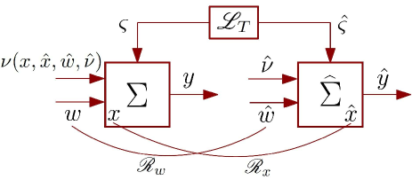
Figure 1. Notion of lifting for specifying the similarity between gMDP and its abstraction. Relations $R_{x}$ and $R_{w}$ are the ones between states and internal inputs, respectively. $\mathscr{L}_{T}$ specifies the relation of two noises, and interface function $\nu_{\hat{\nu}}(x,\hat{x},\hat{w},\hat{\nu})$ is used for the refinement policy.

Definition 3.2 enables us to quantify the error in probability between a concrete system $\Sigma$ and its abstraction $\widehat{\Sigma}$. In any $(\epsilon,\delta)$-approximate probabilistic relation, $\delta$ is used to quantify the distance in probability between gMDPs and $\epsilon$ for the closeness of output trajectories as stated in the next theorem.

Theorem 3.5.

If $\widehat{\Sigma}\preceq_{\epsilon}^{\delta}\Sigma$ and $(w(k),\hat{w}(k))\in\mathscr{R}_{w}$ for all $k\in\{0,1,\ldots,T_{k}\}$, then for all policies on $\widehat{\Sigma}$ there exists a policy for $\Sigma$ such that, for all measurable events $\mathsf{A}\subset Y^{T_{k}+1}$,

$$\mathbb{P}\{\{\hat{y}(k)\}_{0:T_{k}}\in\mathsf{A}^{-\epsilon}\}-\gamma \leq\mathbb{P}\{\{y(k)\}_{0:T_{k}}\in\mathsf{A}\}\leq\mathbb{P}\{\{\hat{y}(k)\}_{0:T_{k}}\in\mathsf{A}^{\epsilon}\}+\gamma,$$ (3.1)

with constant $1-\gamma:=(1-\delta)^{T_{k}+1}$, and with the $\epsilon$-expansion and $\epsilon$-contraction of $\mathsf{A}$ defined as

$$\mathsf{A}^{\epsilon} :=\{y(\cdot)\in Y^{T_{k}+1}\big{|}\exists\bar{y}(\cdot)\in\mathsf{A}\text{ with }max_{k\leq T_{k}}\|\bar{y}(k)-y(k)\|\leq\epsilon\},$$

$$\mathsf{A}^{-\epsilon} :=\{y(\cdot)\in\mathsf{A}\,\,\big{|}\,\,\bar{y}(\cdot)\in\mathsf{A}\text{ for all }\bar{y}(\cdot)\text{ with }max_{k\leq T_{k}}\|\bar{y}(k)-y(k)\|\leq\epsilon\}.$$

We have adapted this theorem from [HSA17] and added its proof in the Appendix for the sake of completeness. We employ this theorem to provide the probabilistic closeness guarantee between interconnected gMDPs and that of their compositional abstractions which are discussed in Section 4.

In the next section, we define composition of gMDPs via their internal inputs and discuss how to relate them to a network of interconnected abstraction based on their individual relations.

4. Interconnected gMDPs and Their Compositional Abstractions

4.1. Interconnected gMDPs

Let $\Sigma$ be a network of $N\in\mathbb{N}_{\geq 1}$ gMDPs

$$\Sigma_{i}=(X_{i},W_{i},U_{i},\pi_{i},T_{i},Y_{i},h_{i}),\quad i\in\{1,\dots,N\}.$$ (4.1)

We partition internal input and output of $\Sigma_{i}$ as

$$w_{i}=[w_{i1};\ldots;w_{i(i-1)};w_{i(i+1)};\ldots;w_{iN}],~{}~{}~{}y_{i}=[y_{i1};\ldots;y_{iN}],$$ (4.2)

and also output space and function as

$$h_{i}(x_{i})=[h_{i1}(x_{i});\ldots;h_{iN}(x_{i})],~{}~{}~{}Y_{i}=\prod_{j=1}^{N}Y_{ij}.$$ (4.3)

The outputs $y_{ii}$ are denoted as external ones, whereas the outputs $y_{ij}$ with $i\neq j$ as internal ones which are employed for interconnection by requiring $w_{ji}=y_{ij}$. This can be explicitly written using appropriate functions $g_{i}$ defined as

$$w_{i}=g_{i}(x_{1},\ldots,x_{N}):=\left[h_{1i}(x_{1});\ldots;h_{(i-1)i}(x_{i-1});h_{(i+1)i}(x_{i+1});\ldots;h_{Ni}(x_{N})\right]\!\!.$$ (4.4)

If there is no connection from $\Sigma_{i}$ to $\Sigma_{j}$, then the connecting output function is identically zero for all arguments, i.e., $h_{ij}\equiv 0$. Now, we define the interconnected gMDP $\Sigma$ as follows.

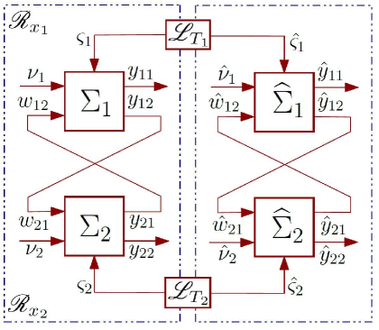
Figure 2. Interconnection of two gMDPs $\Sigma_{1}$ and $\Sigma_{2}$ and that of their abstractions.

Definition 4.1.

Consider $N\in{\mathbb{N}}_{\geq 1}$ gMDPs $\Sigma_{i}=(X_{i},W_{i},U_{i},\pi_{i},T_{i},Y_{i},h_{i}),i\in\{1,\dots,N\}$, with the input-output configuration as in (4.2) and (4.3). The interconnection of $\Sigma_{i}$, $i\in\{1,\dots,N\}$, is a gMDP $\Sigma=(X,U,\pi,T,Y,h)$, denoted by $\mathcal{I}(\Sigma_{1},\ldots,\Sigma_{N})$, such that $X:=\prod_{i=1}^{N}X_{i}$, $U:=\prod_{i=1}^{N}U_{i}$, $Y:=\prod_{i=1}^{N}Y_{ii}$, and $h=\prod_{i=1}^{N}h_{ii}$, with the following constraints:

$$\forall i,j\in\{1,\dots,N\},\,\,i\neq j:\quad w_{ji}=y_{ij},\quad Y_{ij}\subseteq W_{ji}.$$ (4.5)

Moreover, one has conditional stochastic kernel $T:=\prod_{i=1}^{N}T_{i}$ and initial probability distribution $\pi:=\prod_{i=1}^{N}\pi_{i}$.

An example of the interconnection of two gMDPs $\Sigma_{1}$ and $\Sigma_{2}$ and that of their abstractions is illustrated in Figure 2.

Remark 4.2.

Definition 4.1 assumes that uncertainties affecting individual gMDPs in a network $\mathcal{I}(\Sigma_{1},\ldots,\Sigma_{N})$ are independent and, thus, constructs $T$ and $\pi$ by taking products of $T_{i}$ and $\pi_{i}$, respectively. This definition can be generalized for dependent uncertainties by using their joint distribution in the construction of $T$ and $\pi$, in the same manner as we discussed in Remark 3.4 for expressing dependent uncertainties in concrete and abstract gMDPs.

4.2. Compositional Abstractions for Interconnected gMDPs

We assume that we are given $N$ gMDPs as in Definition 2.1 together with their corresponding abstractions $\widehat{\Sigma}_{i}=(\hat{X}_{i},\hat{W}_{i},\hat{U}_{i},\hat{\pi}_{i},\hat{T}_{i},Y_{i},\hat{h}_{i})$ such that $\widehat{\Sigma}_{i}\preceq_{\epsilon_{i}}^{\delta_{i}}\Sigma_{i}$ for some relation $\mathscr{R}_{x_{i}}$ and constants $\epsilon_{i},\delta_{i}$. Next theorem shows the main compositionality result of the paper.

Theorem 4.3.

Consider the interconnected gMDP $\Sigma=\mathcal{I}(\Sigma_{1},\ldots,\Sigma_{N})$ induced by $N\in{\mathbb{N}}_{\geq 1}$ gMDPs $\Sigma_{i}$. Suppose $\widehat{\Sigma}_{i}$ is ($\epsilon_{i},\delta_{i}$)-stochastically simulated by $\Sigma_{i}$ with the corresponding relations $\mathscr{R}_{x_{i}}$ and $\mathscr{R}_{w_{i}}$ and lifting $\mathscr{L}_{i}$. If

$$g_{i}(x)\mathscr{R}_{w_{i}}\hat{g}_{i}(\hat{x}),\quad\forall(x,\hat{x})\in\mathscr{R}_{x_{i}},$$ (4.6)

with interconnection constraint maps $g_{i},\hat{g}_{i}$ defined as in (4.4), then $\widehat{\Sigma}=\mathcal{I}(\widehat{\Sigma}_{1},\ldots,\widehat{\Sigma}_{N})$ is ($\epsilon,\delta$)-stochastically simulated by $\Sigma=\mathcal{I}(\Sigma_{1},\ldots,\Sigma_{N})$ with relation $\mathscr{R}_{x}$ defined as

$$\begin{bmatrix}x_{1}\\ \vdots\\ x_{N}\end{bmatrix}\mathscr{R}_{x}\begin{bmatrix}\hat{x}_{1}\\ \vdots\\ \hat{x}_{N}\end{bmatrix}\Leftrightarrow\left\{\begin{array}[]{l}x_{1}\mathscr{R}_{x_{1}}\hat{x}_{1},\\ ~{}~{}~{}~{}~{}\vdots\\ x_{N}\mathscr{R}_{x_{N}}\hat{x}_{N},\end{array}\right.$$

and constants $\epsilon=\sum_{i=1}^{N}\epsilon_{i}$, and $\delta=1-\prod_{i=1}^{N}(1-\delta_{i})$. Lifting $\mathscr{L}$ and interface $\nu$ are obtained by taking products $\mathscr{L}=\prod_{i=1}^{N}\mathscr{L}_{i}$ and $\nu=\prod_{i=1}^{N}\nu_{i}$, and then substituting interconnection constraints (4.5).

The proof of Theorem 4.3 is provided in the Appendix.

Remark 4.4.

Note that Theorem 4.3 requires $g_{i}(x)\mathscr{R}_{w_{i}}\hat{g}_{i}(\hat{x})$ for any $(x,\hat{x})\in\mathscr{R}_{x}$. This condition puts restriction on the structure of the network and how the dynamics of gMDPs are coupled in the network (cf. Remark 3.3). It is similar to the condition imposed in disturbance bisimulation relation defined in [MSSM16].

We provide the following example to illustrate our compositionality results.

Example 4.5.

Assume that we are given two linear dynamical systems as

$$\Sigma_{i}:\left\{\begin{array}[]{l}x_{i}(k+1)=A_{i}x_{i}(k)+D_{i}w_{i}(k)+B_{i}\nu_{i}(k)+R_{i}\varsigma_{i}(k),\\ y_{i}(k)=x_{i}(k),\quad i\in\{1,2\},\end{array}\right.$$ (4.9)

where the additive noise $\varsigma_{i}(\cdot)$ is a sequence of independent random vectors with multivariate standard normal distributions for $i\in\{1,2\}$, and $R_{i},i\in\{1,2\},$ are invertible. Let $\widehat{\Sigma}_{i}$ be the abstraction of gMDP (4.9) as

$$\widehat{\Sigma}_{i}:\left\{\begin{array}[]{l}\hat{x}_{i}(k+1)=\hat{A}_{i}\hat{x}_{i}(k)+\hat{D}_{i}\hat{w}_{i}(k)+\hat{B}_{i}\hat{\nu}_{i}(k)+\hat{R}_{i}\hat{\varsigma}_{i}(k),\\ \hat{y}_{i}(k)=\hat{x}_{i}(k).\end{array}\right.$$ (4.12)

Transition kernels of $\Sigma_{i}$ and $\widehat{\Sigma}_{i}$ can be written as

$$T_{i}(\cdot|x_{i},w_{i},\nu_{i})=\mathcal{N}(\cdot|A_{i}x_{i}+D_{i}w_{i}+B_{i}\nu_{i},R_{i}R_{i}^{T}),$$

$$\hat{T}_{i}(\cdot|\hat{x}_{i},\hat{w}_{i},\hat{\nu}_{i})=\mathcal{N}(\cdot|\hat{A}_{i}\hat{x}_{i}+\hat{D}_{i}\hat{w}_{i}+\hat{B}_{i}\hat{\nu}_{i},\hat{R}_{i}\hat{R}_{i}^{T}),~{}\forall i\in\{1,2\},$$

where $\mathcal{N}(\cdot\,|\,\mathsf{m},\mathsf{D})$ indicates normal distribution with mean $\mathsf{m}$ and covariance matrix $\mathsf{D}$.

Independent uncertainties. If $\varsigma_{i}(\cdot)$ and $\hat{\varsigma}_{i}(\cdot)$ in the concrete and abstract systems are independent, a candidate for lifted measure is

$$\mathscr{L}_{T_{i}}(\cdot|x_{i},\hat{x}_{i},w_{i},\hat{w}_{i},\hat{\nu}_{i}) =\mathcal{N}(\cdot|A_{i}x_{i}+D_{i}w_{i}+B_{i}\nu_{i},R_{i}R_{i}^{T})\times\mathcal{N}(\cdot|\hat{A}_{i}\hat{x}_{i}+\hat{D}_{i}\hat{w}_{i}+\hat{B}_{i}\hat{\nu}_{i},\hat{R}_{i}\hat{R}_{i}^{T}).$$

Now we connect two subsystems with each other based on the interconnection constraint (4.5) which are $w_{i}=x_{3-i}$ and $\hat{w}_{i}=\hat{x}_{3-i}$ for $i\in\{1,2\}$. For any $x=[{x_{1};x_{2}}]\in X,\hat{x}=[{\hat{x}_{1};\hat{x}_{2}}]\in\hat{X},\nu=[{\nu_{1};\nu_{2}}]\in U,\hat{\nu}=[{\hat{\nu}_{1};\hat{\nu}_{2}}]\in\hat{U}$, the compositional transition kernels for the interconnected gMDPs are

$$T(\cdot~{}|~{}x,\nu)=\mathcal{N}(\cdot~{}|~{}Ax+B\nu,RR^{T}),~{}\hat{T}(\cdot~{}|~{}\hat{x},\hat{\nu})=\mathcal{N}(\cdot~{}|~{}\hat{A}\hat{x}+\hat{B}\hat{\nu},\hat{R}\hat{R}^{T}),$$

where $\nu:=\nu(x,\hat{x},\hat{\nu})$ and

$$A=\begin{bmatrix}A_{1}&D_{1}\\ D_{2}&A_{2}\end{bmatrix}\!\!,\quad B=\mathsf{diag}(B_{1},B_{2}),\quad R=\mathsf{diag}(R_{1},R_{2}),$$

$$\hat{A}=\begin{bmatrix}\hat{A}_{1}&\hat{D}_{1}\\ \hat{D}_{2}&\hat{A}_{2}\end{bmatrix}\!\!,\quad\hat{B}=\mathsf{diag}(\hat{B}_{1},\hat{B}_{2}),\quad\hat{R}=\mathsf{diag}(\hat{R}_{1},\hat{R}_{2}).$$ (4.13)

Then the candidate lifted measure for the interconnected gMDPs is

$$\mathscr{L}_{T}(\cdot|x,\hat{x},\hat{\nu})=\mathcal{N}(\cdot|Ax+B\nu,RR^{T})\mathcal{N}(\cdot|\hat{A}\hat{x}+\hat{B}\hat{\nu},\hat{R}\hat{R}^{T}).$$

Note that after connecting the subsystems with each other using the proposed interconnection constraint in (4.5), the internal inputs will disappear.

Dependent uncertainties. Suppose $\Sigma_{i}$ and $\widehat{\Sigma}_{i}$ share the same noise $\varsigma_{i}(\cdot)=\hat{\varsigma}_{i}(\cdot)$. In this case, the candidate lifted measure for $i\in\{1,2\}$ is obtained by

$$\mathscr{L}_{T_{i}}(dx_{i}^{\prime}\times d\hat{x}_{i}^{\prime}|x_{i},\hat{x}_{i},w_{i},\hat{w}_{i},\hat{\nu}_{i}) =\mathcal{N}(dx_{i}^{\prime}|A_{i}x_{i}+D_{i}w_{i}+B_{i}\nu_{i},R_{i}R_{i}^{T})\times\delta_{d}(d\hat{x}_{i}^{\prime}|\hat{A}_{i}\hat{x}_{i}$$

$$+\hat{D}_{i}\hat{w}_{i}+\hat{B}_{i}\hat{\nu}_{i}+\hat{R}_{i}R_{i}^{-1}(x_{i}^{\prime}-A_{i}x_{i}-D_{i}w_{i}-B_{i}\nu_{i})),$$

where $\delta_{d}(\cdot|\mathsf{a})$ indicates Dirac delta distribution centered at $\mathsf{a}$. Now we connect two subsystems with each other. For any $x=[{x_{1};x_{2}}]\in X,\hat{x}=[{\hat{x}_{1};\hat{x}_{2}}]\in\hat{X},\nu=[{\nu_{1};\nu_{2}}]\in U,\hat{\nu}=[{\hat{\nu}_{1};\hat{\nu}_{2}}]\in\hat{U}$, the candidate lifted measure for the interconnected gMDPs is

$$\mathscr{L}_{T}(dx^{\prime}\times d\hat{x}^{\prime}|x,\hat{x},\hat{\nu})=\mathcal{N} (dx^{\prime}|Ax+B\nu,RR^{T})\times\delta_{d}(d\hat{x}^{\prime}|A\hat{x}+B\hat{\nu}-\bar{A}x+\tilde{A}x^{\prime}-\bar{B}\nu),$$

where $A,B,R,\hat{A},\hat{B}$ are defined as in (4.13), and

$$\bar{A}=\begin{bmatrix}\hat{R}_{1}R_{1}^{-1}A_{1}&\hat{R}_{1}R_{1}^{-1}D_{1}\\ \hat{R}_{2}R_{2}^{-1}D_{2}&\hat{R}_{2}R_{2}^{-1}A_{2}\\ \end{bmatrix}\!\!,\quad\tilde{A}=\begin{bmatrix}\hat{R}_{1}R_{1}^{-1}&0\\ 0&\hat{R}_{2}R_{2}^{-1}\\ \end{bmatrix}\!\!,\quad\bar{B}=\begin{bmatrix}\hat{R}_{1}R_{1}^{-1}B_{1}&0\\ 0&\hat{R}_{2}R_{2}^{-1}B_{2}\\ \end{bmatrix}\!\!.$$

In the next section, we focus on a particular class of stochastic nonlinear systems, and construct its infinite and finite abstractions in a unified framework. We provide explicit inequalities for establishing Theorem 4.3, which gives a probabilistic relation after composition and enables us to get guarantees of Theorem 3.5 on the closeness of the composed system and that of its abstraction.

5. Construction of Abstractions for Nonlinear Systems

Here, we focus on a specific class of stochastic nonlinear control systems $\Sigma$ as

$$\Sigma:\left\{\begin{array}[]{l}x(k+1)=Ax(k)+E\varphi(Fx(k))+Dw(k)+B\nu(k)+R\varsigma(k),\\ y(k)=Cx(k),\end{array}\right.$$ (5.3)

where $\varsigma(\cdot)\sim\mathcal{N}(0,\mathds{I}_{n})$, and $\varphi:{\mathbb{R}}\rightarrow{\mathbb{R}}$ satisfies

$$a\leq\frac{\varphi(c)-\varphi(d)}{c-d}\leq b,~{}~{}~{}\forall c,d\in{\mathbb{R}},c\neq d,$$ (5.4)

for some $a\in{\mathbb{R}}$ and $b\in{\mathbb{R}}_{>0}\cup\{\infty\}$, $a\leq b$.

We use the tuple

$$\Sigma=(A,B,C,D,E,F,R,\varphi),$$

to refer to the class of nonlinear systems of the form (5.3).

Remark 5.1.

If $E$ is a zero matrix or $\varphi$ in (5.3) is linear including the zero function (i.e. $\varphi\equiv 0$), one can remove or push the term $E\varphi(Fx)$ to $Ax$, and consequently the nonlinear tuple reduces to the linear one $\Sigma=(A,B,C,D,R)$. Then, every time we mention the tuple $\Sigma=(A,B,C,D,E,F,R,\varphi)$, it implicitly implies that $\varphi$ is nonlinear and $E$ is nonzero.

Remark 5.2.

Without loss of generality [AK01], we can assume $a=0$ in (5.4) for the class of nonlinear systems in (5.3). If $a\neq 0$, one can define a new function $\tilde{\varphi}(s):=\varphi(s)-as$ satisfying (5.4) with $\tilde{a}=0$ and $\tilde{b}=b-a$, and rewrite (5.3) as

$$\Sigma:\left\{\begin{array}[]{l}x(k+1)=\tilde{A}x(k)+E\tilde{\varphi}(Fx(k))+Dw(k)+B\nu(k)+R\varsigma(k),\\ y(k)=Cx(k)\end{array}\right.$$ (5.7)

where $\tilde{A}=A+aEF$.

Remark 5.3.

We restrict ourselves here to systems with a single nonlinearity as in (5.3) for the sake of simple presentation. However, it would be straightforward to get analogous results for systems with multiple nonlinearities as

$$\Sigma:\left\{\begin{array}[]{l}x(k+1)=Ax(k)+\sum_{i=1}^{\bar{M}}E_{i}\varphi_{i}(F_{i}x(k))+Dw(k)+B\nu(k)+R\varsigma(k),\\ y(k)=Cx(k),\end{array}\right.$$ (5.10)

where $\varphi_{i}:{\mathbb{R}}\rightarrow{\mathbb{R}}$ satisfies (5.4) for some $a_{i}\in{\mathbb{R}}$ and $b_{i}\in{\mathbb{R}}_{>0}\cup\{\infty\}$, for any $i\in\{1,\ldots,\bar{M}\}$.

Existing compositional abstraction results for this class of models are based on either model order reduction [LSMZ17], [LSZ19a] or finite MDPs [LSZ18b], [LSZ18a]. Our proposed results here combine these two approaches in one unified framework. In other words, our abstract model is obtained by discretizing the state space of a reduced-order version of the concrete model.

5.1. Construction of Finite Abstractions

Consider a nonlinear system $\Sigma=(A,B,C,D,E,F,R,\varphi)$ and its reduced-order version $\widehat{\Sigma}_{\textsf{r}}=(\hat{A}_{\textsf{r}},\hat{B}_{\textsf{r}},\hat{C}_{\textsf{r}},\hat{D}_{\textsf{r}},\hat{E}_{\textsf{r}},\hat{F}_{\textsf{r}},\hat{R}_{\textsf{r}},\varphi)$. Note that index r in the whole paper signifies the reduced-order version of the original model. We discuss the construction of $\widehat{\Sigma}_{\textsf{r}}$ from $\Sigma$ in Theorem 5.5 of the next subsection. Construction of a finite gMDP from $\widehat{\Sigma}_{\textsf{r}}$ follows the approach of [Sou14, SA13]. Denote the state and input spaces of $\widehat{\Sigma}_{\textsf{r}}$ respectively by $\hat{X}_{\textsf{r}},\hat{W}_{\textsf{r}},\hat{U}_{\textsf{r}}$. We construct a finite gMDP by selecting partitions $\hat{X}_{\textsf{r}}=\cup_{i}\mathsf{X}_{i}$, $\hat{W}_{\textsf{r}}=\cup_{i}\mathsf{W}_{i}$, and $\hat{U}_{\textsf{r}}=\cup_{i}\mathsf{U}_{i}$, and choosing representative points $\bar{x}_{i}\in\mathsf{X}_{i}$, $\bar{w}_{i}\in\mathsf{W}_{i}$, and $\bar{\nu}_{i}\in\mathsf{U}_{i}$, as abstract states and inputs. The finite abstraction of $\Sigma$ is a gMDP $\widehat{\Sigma}=(\hat{X},\hat{W},\hat{U},\hat{\pi},\hat{T},Y,\hat{h})$, where

$$\hat{X}=\{\bar{x}_{i},i=1,\ldots,n_{x}\},~{}\hat{U}=\{\bar{u}_{i},i=1,\ldots,n_{u}\},~{}\hat{W}=\{\bar{w}_{i},i=1,\ldots,n_{w}\}.$$

Transition probability matrix $\hat{T}$ is constructed according to the dynamics $\hat{x}(k+1)=\hat{f}(\hat{x}(k),\hat{w}(k),\hat{\nu}(k),\varsigma(k))$ with

$$\hat{f}(\hat{x},\hat{\nu},\hat{w},\varsigma):=\Pi_{x}(\hat{A}_{\textsf{r}}\hat{x}+\hat{E}_{\textsf{r}}\varphi(\hat{F}_{\textsf{r}}\hat{x})+\hat{D}_{\textsf{r}}\hat{w}+\hat{B}_{\textsf{r}}\hat{\nu}+\hat{R}_{\textsf{r}}\varsigma),$$ (5.11)

where $\Pi_{x}:\hat{X}_{\textsf{r}}\rightarrow\hat{X}$ is the map that assigns to any $\hat{x}_{\textsf{r}}\in\hat{X}_{\textsf{r}}$, the representative point $\hat{x}\in\hat{X}$ of the corresponding partition set containing $\hat{x}_{\textsf{r}}$. The output map $\hat{h}(\hat{x})=\hat{C}\hat{x}$. The initial state of $\widehat{\Sigma}$ is also selected according to $\hat{x}_{0}:=\Pi_{x}(\hat{x}_{\textsf{r}}(0))$ with $\hat{x}_{\textsf{r}}(0)$ being the initial state of $\widehat{\Sigma}_{\textsf{r}}$.

Remark 5.4.

Abstraction map $\Pi_{x}$ satisfies the inequality $\|\Pi_{x}(\hat{x}_{\textsf{r}})-\hat{x}_{\textsf{r}}\|\leq\beta$ for all $\hat{x}_{\textsf{r}}\,\in\hat{X}_{\textsf{r}},$ where $\beta$ is the state discretization parameter defined as $\beta:=\sup\{\|\hat{x}_{\textsf{r}}-\hat{x}_{\textsf{r}}^{\prime}\|,\,\,\hat{x}_{\textsf{r}},\hat{x}_{\textsf{r}}^{\prime}\in\mathsf{X}_{i},\,i=1,2,\ldots,n_{x}\}$.

5.2. Establishing Probabilistic Relations

In this subsection, we provide conditions under which $\widehat{\Sigma}$ is ($\epsilon,\delta$)-stochastically simulated by $\Sigma$, i.e. $\widehat{\Sigma}\preceq_{\epsilon}^{\delta}\Sigma$, with relations $\mathscr{R}_{x}$ and $\mathscr{R}_{w}$. Here we candidate relations

$$\halign to=0.0pt{\relax\global\advance\@IEEEeqncolcnt by 1\relax\begingroup\csname @IEEEeqnarraycolPREr\endcsname#\relax\relax\relax\relax\relax\relax\relax\relax\relax\relax\csname @IEEEeqnarraycolPOSTr\endcsname\relax\relax\relax\relax\relax\relax\relax\relax\relax\relax\endgroup&\relax\global\advance\@IEEEeqncolcnt by 1\relax\begingroup\csname @IEEEeqnarraycolPREC\endcsname#\relax\relax\relax\relax\relax\relax\relax\relax\relax\relax\csname @IEEEeqnarraycolPOSTC\endcsname\relax\relax\relax\relax\relax\relax\relax\relax\relax\relax\endgroup&\relax\global\advance\@IEEEeqncolcnt by 1\relax\begingroup\csname @IEEEeqnarraycolPREl\endcsname#\relax\relax\relax\relax\relax\relax\relax\relax\relax\relax\csname @IEEEeqnarraycolPOSTl\endcsname\relax\relax\relax\relax\relax\relax\relax\relax\relax\relax\endgroup&\global\advance\@IEEEeqncolcnt by 1\relax\bgroup#\egroup&\global\advance\@IEEEeqncolcnt by 1\relax\hbox to\z@\bgroup\hss#\egroup\cr\hfil$\displaystyle \mathscr{R}_{x}$&\hfil$\displaystyle{}={}$\hfil&$\displaystyle\Big{\{}(x,\hat{x})|(x-P\hat{x})^{T}M(x-P\hat{x})\leq\epsilon^{2}\Big{\}},$\hfil&{{}\vrule width=0.0pt,height=0.0pt,depth=0.0pt}&0.0pt{\hss(5.12a)}\cr\penalty 100\vskip 3.0pt\vskip 0.0pt\cr\hfil$\displaystyle \mathscr{R}_{w}$&\hfil$\displaystyle{}={}$\hfil&$\displaystyle\Big{\{}(w,\hat{w})|(w-P_{w}\hat{w})^{T}M_{w}(w-P_{w}\hat{w})\leq\epsilon_{w}^{2}\Big{\}}, $\hfil&{\vrule width=0.0pt,height=0.0pt,depth=0.0pt}&0.0pt{\hss(5.12b)}\cr}$$

where $P\in\mathbb{R}^{n\times\hat{n}}$ and $P_{w}\in\mathbb{R}^{m\times\hat{m}}$ are matrices of appropriate dimensions (potentially with the lowest $\hat{n}$ and $\hat{m}$), and $M,M_{w}$ are positive-definite matrices.

Next theorem gives conditions for having $\widehat{\Sigma}\preceq_{\epsilon}^{\delta}\Sigma$ with relations (5.2) and (5.2).

Theorem 5.5.

Let $\Sigma=(A,B,C,D,E,F,R,\varphi)$ and $\widehat{\Sigma}_{\textsf{r}}=(\hat{A}_{\textsf{r}},\hat{B}_{\textsf{r}},\hat{C}_{\textsf{r}},\hat{D}_{\textsf{r}},\hat{E}_{\textsf{r}},\hat{F}_{\textsf{r}},\hat{R}_{\textsf{r}},\varphi)$ be two nonlinear systems with the same additive noise. Suppose $\widehat{\Sigma}$ is a finite gMDP constructed from $\widehat{\Sigma}_{\textsf{r}}$ according to subsection 5.1. Then $\widehat{\Sigma}$ is ($\epsilon,\delta$)-stochastically simulated by $\Sigma$ with relations (5.2)-(5.2) if there exist matrices $K$, $Q$, $S$, $L_{1}$, $L_{2}$ and $\tilde{R}$ such that

$$\halign to=0.0pt{\relax\global\advance\@IEEEeqncolcnt by 1\relax\begingroup\csname @IEEEeqnarraycolPREr\endcsname#\relax\relax\relax\relax\relax\relax\relax\relax\relax\relax\csname @IEEEeqnarraycolPOSTr\endcsname\relax\relax\relax\relax\relax\relax\relax\relax\relax\relax\endgroup&\relax\global\advance\@IEEEeqncolcnt by 1\relax\begingroup\csname @IEEEeqnarraycolPREC\endcsname#\relax\relax\relax\relax\relax\relax\relax\relax\relax\relax\csname @IEEEeqnarraycolPOSTC\endcsname\relax\relax\relax\relax\relax\relax\relax\relax\relax\relax\endgroup&\relax\global\advance\@IEEEeqncolcnt by 1\relax\begingroup\csname @IEEEeqnarraycolPREl\endcsname#\relax\relax\relax\relax\relax\relax\relax\relax\relax\relax\csname @IEEEeqnarraycolPOSTl\endcsname\relax\relax\relax\relax\relax\relax\relax\relax\relax\relax\endgroup&\global\advance\@IEEEeqncolcnt by 1\relax\bgroup#\egroup&\global\advance\@IEEEeqncolcnt by 1\relax\hbox to\z@\bgroup\hss#\egroup\cr\hfil$\displaystyle M$&\hfil$\displaystyle{}\succeq{}$\hfil&$\displaystyle C^{T}C ,$\hfil&{{}\vrule width=0.0pt,height=0.0pt,depth=0.0pt}&0.0pt{\hss(5.13a)}\cr\penalty 100\vskip 3.0pt\vskip 0.0pt\cr\hfil$\displaystyle \hat{C}_{{r}}$&\hfil$\displaystyle{}={}$\hfil&$\displaystyle CP,$\hfil&{{}\vrule width=0.0pt,height=0.0pt,depth=0.0pt}&0.0pt{\hss(5.13b)}\cr\penalty 100\vskip 3.0pt\vskip 0.0pt\cr\hfil$\displaystyle \hat{F}_{{r}}$&\hfil$\displaystyle{}={}$\hfil&$\displaystyle FP,$\hfil&{{}\vrule width=0.0pt,height=0.0pt,depth=0.0pt}&0.0pt{\hss(5.13c)}\cr\penalty 100\vskip 3.0pt\vskip 0.0pt\cr\hfil$\displaystyle E$&\hfil$\displaystyle{}={}$\hfil&$\displaystyle P\hat{E}_{{r}}-B(L_{1}-L_{2}),$\hfil&{{}\vrule width=0.0pt,height=0.0pt,depth=0.0pt}&0.0pt{\hss(5.13d)}\cr\penalty 100\vskip 3.0pt\vskip 0.0pt\cr\hfil$\displaystyle AP$&\hfil$\displaystyle{}={}$\hfil&$\displaystyle P\hat{A}_{{r}}-BQ,$\hfil&{{}\vrule width=0.0pt,height=0.0pt,depth=0.0pt}&0.0pt{\hss(5.13e)}\cr\penalty 100\vskip 3.0pt\vskip 0.0pt\cr\hfil$\displaystyle DP_{w}$&\hfil$\displaystyle{}={}$\hfil&$\displaystyle P\hat{D}_{{r}}-BS,$\hfil&{{}\vrule width=0.0pt,height=0.0pt,depth=0.0pt}&0.0pt{\hss(5.13f)}\cr\penalty 100\vskip 3.0pt\vskip 0.0pt\cr\hfil$\displaystyle \mathbb{P}\{(H+PG)^{T}M(H$&\hfil$\displaystyle{}+{}$\hfil&$\displaystyle PG)\leq\epsilon^{2}\} \succeq 1-\delta, $\hfil&{\vrule width=0.0pt,height=0.0pt,depth=0.0pt}&0.0pt{\hss(5.13g)}\cr}$$

where

$$H =((A+BK)+\bar{\delta}(BL_{1}+E)F)(x-P\hat{x})+D(w-P_{w}\hat{w})+(B\tilde{R}-P\hat{B}_{\textsf{r}})\hat{\nu}+(R-P\hat{R}_{\textsf{r}})\varsigma,$$

$$G =\hat{A}_{\textsf{r}}\hat{x}+\hat{E}_{\textsf{r}}\varphi(\hat{F}_{\textsf{r}}\hat{x})+\hat{D}_{\textsf{r}}\hat{w}+\hat{B}_{\textsf{r}}\hat{\nu}+\hat{R}_{\textsf{r}}\varsigma-\Pi_{x}(\hat{A}_{\textsf{r}}\hat{x}+\hat{E}_{\textsf{r}}\varphi(\hat{F}_{\textsf{r}}\hat{x})+\hat{D}_{\textsf{r}}\hat{w}+\hat{B}_{\textsf{r}}\hat{\nu}+\hat{R}_{\textsf{r}}\varsigma).$$

The proof of Theorem 5.5 is provided in the Appendix.

Remark 5.6.

Note that condition (5.5) is a chance constraint. We satisfy this condition by selecting constant $c_{\varsigma}$ such that $\mathbb{P}\{\varsigma^{T}\varsigma\leq c_{\varsigma}^{2}\}\geq 1-\delta$, and requiring $(H+PG)^{T}M(H+PG)\leq\epsilon^{2}$ for any $\varsigma$ with $\varsigma^{T}\varsigma\leq c_{\varsigma}^{2}$. Since $\varsigma\sim(0,\mathds{I}_{n})$, $\varsigma^{T}\varsigma$ has chi-square distribution with $2$ degrees of freedom. Thus, $c_{\varsigma}=\mathcal{X}_{2}^{-1}(1-\delta)$ with $\mathcal{X}_{2}^{-1}$ being chi-square inverse cumulative distribution function with $2$ degrees of freedom.

6. Case Study

In this section, we demonstrate the effectiveness of the proposed results on a network of four stochastic nonlinear systems (totally 12 dimensions), i.e. $\Sigma=\mathcal{I}(\Sigma_{1},\Sigma_{2},\Sigma_{3},\Sigma_{4})$. We want to construct finite gMDPs from their reduced-order versions (together 4 dimensions). The interconnected gMDP $\Sigma$ is illustrated in Figure 3 such that the output of $\Sigma_{1}$ (resp. $\Sigma_{2}$) is connected to the internal input of $\Sigma_{4}$ (resp. $\Sigma_{3}$), and the output of $\Sigma_{3}$ (resp. $\Sigma_{4}$) connects to the internal input of $\Sigma_{1}$ (resp. $\Sigma_{2}$).

The matrices of the system are given by

$$A_{i}=\begin{bmatrix}0.7882&0.3956&0.8333\\ 0.7062&0.7454&0.9552\\ 0.6220&0.3116&0.4409\\ \end{bmatrix}\!\!,\quad B_{i}=\begin{bmatrix}0.7555&0.1557&0.3487\\ 0.1271&0.9836&0.2030\\ 0.4735&0.4363&0.4493\\ \end{bmatrix}\!\!,\quad C_{i}=0.01\mathds{1}_{3}^{T},$$

$$E_{i}=\begin{bmatrix}0.6482;\!&\!0.6008;\!&\!0.6209\end{bmatrix}\!\!,\quad F_{i}=\begin{bmatrix}0.5146;\!&\!0.8756;\!&\!0.2461\end{bmatrix}^{T}\!\!\!\!\!,\quad R_{i}=\begin{bmatrix}0.4974;\!&\!0.3339;\!&\!0.4527\end{bmatrix}\!\!,$$ (6.1)

for $i\in\{1,2,3,4\}$. The internal input and output matrices are also given by

$$C_{14}=C_{23}=C_{31}=C_{42}=0.01\mathds{1}_{3}^{T}\!,\quad D_{13}=D_{24}=D_{32}=D_{41}\!=\!\begin{bmatrix}0.074;\!&\!0.010;\!&\!0.086\end{bmatrix}\!\!.$$

We consider $\varphi_{i}(x)=sin(x)$, $\forall i\in\{1,\ldots,4\}$. Then functions $\varphi_{i}$ satisfy condition (5.4) with $b=1$. In the following, we first construct the reduced-order version of the given dynamic by satisfying conditions  (5.5)-(5.5). We then establish relations between subsystems by fulfilling condition (5.5). Afterwards, we satisfy the compositionality condition (4.6) to get a relation on the composed system, and finally, we utilize Theorem 3.5 to provide the probabilistic closeness guarantee between the interconnected model and its constructed finite MDP.

Conditions (5.5)-(5.5) are satisfied with, $\forall i\in\{1,2,3,4\}$,

$$Q_{i} =\begin{bmatrix}-1.6568;\!&\!-1.2280;\!&\!1.9276\end{bmatrix}\!\!,\quad S_{i}=\begin{bmatrix}0.0775;\!&\!0.0726;\!&\!-0.1759\end{bmatrix}\!\!,$$

$$P_{i} =\begin{bmatrix}0.5931;\!&\!0.3981;\!&\!0.5398\end{bmatrix}\!\!,\quad L_{1i}=\begin{bmatrix}-0.6546;\!&\!-0.4795;\!&\!-0.2264\end{bmatrix}\!\!,$$

$$L_{2i} =\begin{bmatrix}-0.1713;\!&\!-0.0777;\!&\!-0.1044\end{bmatrix}\!\!,\quad P_{wi}=1,M_{i}=\mathds{I}_{3}.$$

Figure 3. The interconnected gMDP $\Sigma=\mathcal{I}(\Sigma_{1},\Sigma_{2},\Sigma_{3},\Sigma_{4})$.

Accordingly, matrices of reduced-order systems can be obtained as $,\forall i\in\{1,2,3,4\},$

$$\hat{A}_{{\textsf{r}}i}=0.5127,\hat{E}_{{\textsf{r}}i}=0.3,\hat{F}_{{\textsf{r}}i}=0.7866,\hat{C}_{{\textsf{r}}i}=0.0371,\hat{D}_{{\textsf{r}}i}=0.1403,\hat{R}_{{\textsf{r}}i}=0.8386.$$

Moreover, we compute $\tilde{R}_{i}=(B_{i}^{T}M_{i}B_{i})^{-1}B_{i}^{T}M_{i}P_{i}\hat{B}_{{\textsf{r}}i}$, $i\in\{1,2,3,4\}$, to make chance constraint (5.5) less conservative. By taking $\hat{B}_{{\textsf{r}}i}=2$, we have $\tilde{R}_{i}=[1.1418;0.5182;0.6965]$. The interface functions for $i\in\{1,2,3,4\}$ are acquired by (9.3) as

$$\nu_{i}= \begin{bmatrix}-0.6665\,&\,-0.3652\,&\,-0.9680\\ -0.4372\,&\,-0.5536\,&\,-0.5781\\ -0.4012\,&\,-0.1004\,&\,-0.2612\\ \end{bmatrix}\!\!(x_{i}-P_{i}\hat{x}_{i})+Q_{i}\hat{x}_{i}+\tilde{R}_{i}\hat{\nu}_{i}+S_{i}\hat{w}_{i}+L_{1i}\varphi_{i}(F_{i}x_{i})-L_{2i}\varphi_{i}(F_{i}P_{i}\hat{x}_{i}).$$

We proceed with showing that condition (5.5) holds as well, using Remark 5.6. This condition can be satisfied via the S-procedure [BV04], which enables us to reformulate (5.5) as existence of $\lambda\geq 0$ such that matrix inequality

$$\lambda_{i}\begin{bmatrix}\tilde{F}_{1i}&\tilde{g}_{1i}\\ \tilde{g}_{1i}^{T}&\tilde{h}_{1i}\\ \end{bmatrix}\!\!-\begin{bmatrix}\tilde{F}_{2i}&\tilde{g}_{2i}\\ \tilde{g}_{2i}^{T}&\tilde{h}_{2i}\\ \end{bmatrix}\!\succeq 0,$$ (6.2)

holds. Here, $\tilde{F}_{1i}$ and $\tilde{F}_{2i}$ are symmetric matrices, $\tilde{g}_{1i}$ and $\tilde{g}_{2i}$ are vectors, $\tilde{h}_{1i}$ and $\tilde{h}_{2i}$ are real numbers. We first bound the external input of abstract systems as $\hat{\nu}_{i}^{2}\leq c_{\hat{\nu}i}$ and select $c_{\varsigma i}=\mathcal{X}_{2}^{-1}(1-\delta_{i})$, for all $i\in\{1,2,3,4\}$. Then matrices, vectors and real numbers of inequality (6.2), $\forall i\in\{1,2,3,4\}$, can be constructed as in (9.1) and (9) provided in the Appendix. By taking $\epsilon_{i}=1.25$, $\epsilon_{w_{i}}=0.05$, $c_{\hat{\nu}_{i}}=0.25$, $\delta_{i}=0.001$, $\beta_{i}=0.1$, $\lambda_{i}=0.347$, for all $i\in\{1,2,3,4\}$, one can readily verify that the matrix inequality (6.2) holds. Then $\widehat{\Sigma}_{i}$ is ($\epsilon_{i},\delta_{i}$)-stochastically simulated by $\Sigma_{i}$ with relations

$$\mathscr{R}_{xi}=\Big{\{}(x_{i},\hat{x}_{i})~{}|~{}(x_{i}-P_{i}\hat{x}_{i})^{T}M_{i}(x_{i}-P_{i}\hat{x}_{i})\leq\epsilon_{i}^{2}\Big{\}},\quad\mathscr{R}_{wi}=\Big{\{}(w_{i},\hat{w}_{i})~{}|~{}(w_{i}-\hat{w}_{i})^{2}\leq\epsilon_{wi}^{2}\Big{\}},$$

for $i\in\{1,2,3,4\}$. We proceed with showing that the compositionality condition in (4.6) holds, as well. To do so, by employing S-procedure, one should satisfy the matrix inequality in (6.2) with the following matrices:

$$\tilde{F}_{1i}=\begin{bmatrix}M_{i}&-M_{i}P_{i}\\ *&P_{i}^{T}M_{i}P_{i}\\ \end{bmatrix}\!\!,\quad\tilde{F}_{2i}=\begin{bmatrix}C_{{\textsf{r}}i}^{T}M_{wi}C_{{\textsf{r}}i}&-C_{{\textsf{r}}i}^{T}M_{wi}P_{wi}\hat{C}_{{\textsf{r}}i}\\ *&\hat{C}_{{\textsf{r}}i}^{T}P_{wi}^{T}M_{wi}P_{wi}\hat{C}_{{\textsf{r}}i}\\ \end{bmatrix}\!\!,$$

$$\tilde{g}_{1i}=\tilde{g}_{2i}=\mathbf{0}_{4},\quad\tilde{h}_{1i}=-\epsilon_{i}^{2},\tilde{h}_{2i}=-\epsilon_{wi}^{2},$$

for $i\in\{1,2,3,4\}$. This condition is satisfiable with $\lambda_{i}=0.001~{}\forall i\in\{1,2,3,4\}$, thus $\widehat{\Sigma}$ is ($\epsilon,\delta$)-stochastically simulated by $\Sigma$ with $\epsilon=6$, and $\delta=0.003$. According to (3.1), we guarantee that the distance between outputs of $\Sigma$ and of $\widehat{\Sigma}$ will not exceed $\epsilon=6$ during the time horizon $T_{k}=10$ with probability at least $96\%$ ($\gamma=0.04$).

6.1. Comparison

To demonstrate the effectiveness of the proposed approach, let us now compare the guarantees provided by our approach and by [LSZ19a, LSZ18b]. Note that our result is based on the $\delta$-lifted relation while [LSZ19a, LSZ18b] employ dissipativity-type reasoning to provide a compositional methodology for constructing both infinite abstractions (reduced-order models) and finite MDPs in two consecutive steps. Since we are not able to satisfy the proposed matrix inequalities in [LSZ18b, Ineqality (22)], and [LSZ19a, Inequality (5.5)] for the given system in (6.1), we change the system dynamics to have a fair comparison. In other words, in order to show the conservatism nature of the existing techniques in [LSZ18b, LSZ19a], we provide another example and compare our techniques with the existing ones in great detail.

The matrices of the new system are given by

$$A_{i}=\mathds{I}_{5},~{}B_{i}=\mathds{I}_{5},~{}C_{i}=0.05\mathds{1}_{5}^{T},~{}R_{i}=\mathds{1}_{5},$$

for $i\in\{1,2,3,4\}$, where matrices $E_{i},F_{i}$ are identically zero. The internal input and output matrices are also given by:

$$C_{14}=C_{23}=C_{31}=C_{42}=0.05\mathds{1}_{5}^{T},\quad D_{13}=D_{24}=D_{32}=D_{41}=0.1\mathds{1}_{5}.$$

Conditions (5.5),(5.5),(5.5),(5.5) are satisfied by:

$$M_{i}=\mathds{I}_{5},~{}P_{xi}=\mathds{1}_{5},~{}P_{wi}=1,~{}Q_{i}=\mathds{1}_{5},~{}S_{i}=0.1\mathds{1}_{5},$$

for $i\in\{1,2,3,4\}$. Accordingly, the matrices of reduced-order systems are given as:

$$\hat{A}_{{\textsf{r}}i}=2,\hat{C}_{{\textsf{r}}i}=0.25,\hat{D}_{{\textsf{r}}i}=0.2,\hat{R}_{{\textsf{r}}i}=0.97,~{}\forall i\in\{1,2,3,4\}.$$

Moreover, by taking $\hat{B}_{{\textsf{r}}i}=1$, we compute $\tilde{R}_{i}$, $i\in\{1,2,3,4\}$, as $\tilde{R}_{i}=\mathds{1}_{5}$. The interface function for $i\in\{1,2,3,4\}$ is computed as:

$$\nu_{i}=-0.95\mathds{I}_{5}(x_{i}-\mathds{1}_{5}\hat{x}_{i})+\mathds{1}_{5}\hat{x}_{i}+\mathds{1}_{5}\hat{\nu}_{i}+0.1\mathds{1}_{5}\hat{\omega}_{i}.$$

We proceed with showing that condition (5.5) holds, as well. By taking

$$\epsilon_{i}=5,\epsilon_{w_{i}}=0.75,c_{\hat{\nu}_{i}}=0.25,\delta_{i}=0.001,\beta_{i}=0.1,\lambda_{i}=0.825,\quad\forall i\in\{1,2,3,4\},$$

and by employing S-procedure, one can readily verify that condition (5.5) holds. Then $\widehat{\Sigma}_{i}$ is ($\epsilon_{i},\delta_{i}$)-stochastically simulated by $\Sigma_{i}$, for $i\in\{1,2,3,4\}$. Additionally, by applying S-procedure, one can readily verify that $\widehat{\Sigma}$ is ($\epsilon,\delta$)-stochastically simulated by $\Sigma$ with $\epsilon=20$, and $\delta=0.005$. According to (3.1), we guarantee that the distance between outputs of $\Sigma$ and of $\widehat{\Sigma}$ will not exceed $\epsilon=20$ during the time horizon $T_{k}=5$ with probability at least $97\%$ ($\gamma=0.03$).

Now we apply the proposed results in [LSZ18b, LSZ19a] for the same matrices of the new system and also employing the same $\epsilon$ and discretization parameter $\beta$. Since the proposed approaches in [LSZ18b, LSZ19a] are presented in two consecutive steps, we employ the next proposition which provides the overall error bound in two-step abstraction scheme.

Proposition 6.1.

Suppose $\Sigma_{1}$, $\Sigma_{2}$, and $\Sigma_{3}$ are three stochastic systems without internal signals. For any external input trajectories $\nu_{1}$, $\nu_{2}$, and $\nu_{3}$ and for any $a_{1}$, $a_{2}$, and $a_{3}$ as the initial states of the three systems, if

$$\mathbb{P}\left\{\sup_{0\leq k\leq T_{k}}\|y_{1a_{1}\nu_{1}}(k)-y_{2a_{2}\nu_{2}}(k)\|\geq\epsilon_{1}\,|\,[a_{1};a_{2}]\right\}\leq\gamma_{1},$$

$$\mathbb{P}\left\{\sup_{0\leq k\leq T_{k}}\|y_{2a_{2}\nu_{2}}(k)-y_{3a_{3}\nu_{3}}(k)\|\geq\epsilon_{2}\,|\,[a_{2};a_{3}]\right\}\leq\gamma_{2},$$

for some $\epsilon_{1},\epsilon_{2}>0$ and $\gamma_{1},\gamma_{2}\in]0~{}1[$, then the probabilistic mismatch between output trajectories of $\Sigma_{1}$ and $\Sigma_{3}$ is quantified as

$$\mathbb{P} \left\{\sup_{0\leq k\leq T_{k}}\|y_{1a_{1}\nu_{1}}(k)-y_{3a_{3}\nu_{3}}(k)\|\geq\epsilon_{1}+\epsilon_{2}\,|\,[a_{1};a_{2};a_{3}]\right\}\leq\gamma_{1}+\gamma_{2}.$$

The proof is provided in the Appendix.

By applying the proposed results in [LSZ19a] to construct the infinite abstraction $\widehat{\Sigma}_{\textsf{r}}$, one can guarantee that the distance between outputs of $\Sigma$ and of $\widehat{\Sigma}_{\textsf{r}}$ will exceed $\epsilon_{1}=15$ during the time horizon $T_{k}=5$ with probability at most $87.94\%$, i.e.,

$$\mathbb{P}(\|y_{a\nu}(k)-\hat{y}_{{\textsf{r}}\hat{a}_{\textsf{r}}\hat{\nu}_{\textsf{r}}}(k)\|\geq 15,\,\,\forall k\in[0,5])\leq 87.94\,.$$

After applying the proposed results in [LSZ18b] to construct the finite abstraction $\widehat{\Sigma}$ from $\widehat{\Sigma}_{\textsf{r}}$, one can guarantee that the distance between outputs of $\widehat{\Sigma}_{\textsf{r}}$ and of $\widehat{\Sigma}$ will exceed $\epsilon_{2}=5$ during the time horizon $T_{k}=5$ with probability at most $0.0117\%$, i.e.,

$$\mathbb{P}(\|\hat{y}_{{\textsf{r}}\hat{a}_{\textsf{r}}\hat{\nu}_{\textsf{r}}}(k)-\hat{y}_{\hat{a}\hat{\nu}}(k)\|\geq 5,\,\,\forall k\in[0,5])\leq 0.0117.$$

By employing Proposition 6.1, one can guarantee that the distance between outputs of $\Sigma$ and of $\widehat{\Sigma}$ will exceed $\epsilon=20$ during the time horizon $T_{k}=5$ with probability at most $0.8911\%$, i.e.

$$\mathbb{P}(\|y_{a\nu}(k)-\hat{y}_{\hat{a}\hat{\nu}}(k)\|\geq 20,\,\,\forall k\in[0,5])\leq 0.8911.$$

This means that the distance between outputs of $\Sigma$ and of $\widehat{\Sigma}$ will not exceed $\epsilon=20$ during the time horizon $T_{k}=5$ with probability at least $0.1089\%$. As seen, our provided results dramatically outperform the ones proposed in [LSZ18b, LSZ19a]. More precisely, since our proposed approach here is presented in a unified framework than two-step abstraction scheme which is the case in [LSZ18b, LSZ19a], we only need to check our proposed conditions one time, and consequently, our proposed approach here is much less conservative.

7. Discussion

In this paper, we provided a unified compositional scheme for constructing both finite and infinite abstractions of gMDPs with internal inputs. We defined ($\epsilon,\delta$)-approximate probabilistic relations that are suitable for constructing compositional abstractions of gMDPs. We focused on a specific class of nonlinear dynamical systems, and constructed both infinite (reduced-order models) and finite abstractions in a unified framework, using quadratic relations on the space and linear interface functions. We then provided conditions for composing such relations. Finally, we demonstrated the effectiveness of the proposed results by considering a network of four nonlinear systems (totally 12 dimensions) and constructing finite gMDPs from their reduced-order versions (together 4 dimensions) with guaranteed bounds on their probabilistic output trajectories. We benchmarked our results against the compositional abstraction techniques of [LSZ18b, LSZ19a], and showed that our proposed approach is much less conservative than the ones proposed in [LSZ18b, LSZ19a].

8. Acknowledgment

This work was supported in part by the H2020 ERC Starting Grant AutoCPS (grant agreement No. 804639).

9. Appendix

Definition 9.1.

([HSA17]) Consider two gMDPs without internal inputs $\Sigma=(X,U,\pi,T,Y,h)$ and $\widehat{\Sigma}=(\hat{X},\hat{U},\hat{\pi},\hat{T},Y,\hat{h})$, that have the same output spaces. $\widehat{\Sigma}$ is ($\epsilon,\delta$)-stochastically simulated by $\Sigma$, i.e. $\widehat{\Sigma}\preceq_{\epsilon}^{\delta}\Sigma$, if there exists a relation $\mathscr{R}_{x}\subseteq X\times\hat{X}$ for which there exists a Borel measurable stochastic kernel $\mathscr{L}_{T}(\cdot~{}|~{}x,\hat{x},\hat{\nu})$ on $X\times\hat{X}$ such that

• $\forall(x,\hat{x})\in\mathscr{R}_{x},~{}\|h(x)-\hat{h}(\hat{x})\|\leq\epsilon$,

• $\forall(x,\hat{x})\in\mathscr{R}_{x},\forall\hat{\nu}\in\hat{U},\exists\nu\in U~{}~{}~{}$ ​​​​​ such that $T(\cdot~{}|~{}x,\nu(x,\hat{x},\hat{\nu}))~{}\mathscr{\bar{R}}_{\delta}~{}\hat{T}(\cdot~{}|~{}\hat{x},\hat{\nu})$ with $\mathscr{L}_{T}(\cdot~{}|~{}x,\hat{x},\hat{\nu})$,

• $\pi~{}\mathscr{\bar{R}}_{\delta}~{}\hat{\pi}$.

Matrices appeared in (6.2):

$$\tilde{F}_{1i}=\begin{bmatrix}M_{i}&\mathbf{0}_{3\times 3}&\mathbf{0}_{3}&\mathbf{0}_{3}&\mathbf{0}_{3}&\mathbf{0}_{3}\\ \mathbf{0}_{3\times 3}&\mathbf{0}_{3\times 3}&\mathbf{0}_{3}&\mathbf{0}_{3}&\mathbf{0}_{3}&\mathbf{0}_{3}\\ *&*&M_{wi}&0&0&0\\ *&*&*&1&0&0\\ *&*&*&*&1&0\\ *&*&*&*&*&1\\ \end{bmatrix}\!\!,\quad\tilde{F}_{2i}=\begin{bmatrix}\tilde{F}_{11i}&\tilde{F}_{12i}&\tilde{F}_{13i}&\tilde{F}_{14i}&\tilde{F}_{15i}&\tilde{F}_{16i}\\ *&\tilde{F}_{22i}&\tilde{F}_{23i}&\tilde{F}_{24i}&\tilde{F}_{25i}&\tilde{F}_{26i}\\ *&*&\tilde{F}_{33i}&\tilde{F}_{34i}&\tilde{F}_{35i}&\tilde{F}_{36i}\\ *&*&*&\tilde{F}_{44i}&\tilde{F}_{45i}&\tilde{F}_{46i}\\ *&*&*&*&\tilde{F}_{55i}&\tilde{F}_{56i}\\ *&*&*&*&*&\tilde{F}_{66i}\\ \end{bmatrix}\!\!,$$ (9.1)

where

$$\tilde{F}_{11i}\!=\!(A_{i}\!+\!B_{i}K_{i})^{T}M_{i}(A_{i}\!+\!B_{i}K_{i}),\tilde{F}_{12i}\!=\!(A_{i}\!+\!B_{i}K_{i})^{T}M_{i}(B_{i}L_{1i}\!+\!E_{i})F_{i},\tilde{F}_{13i}\!=\!(A_{i}\!+\!B_{i}K_{i})^{T}M_{i}D_{i},$$

$$\tilde{F}_{14i}\!=\!(A_{i}\!+\!B_{i}K_{i})^{T}M_{i}(B_{i}\tilde{R}_{i}\!-\!P_{i}\hat{B}_{{\textsf{r}}i}),\tilde{F}_{15i}\!=\!(A_{i}\!+\!B_{i}K_{i})^{T}M_{i}P_{i},\tilde{F}_{16i}\!=\!(A_{i}\!+\!B_{i}K_{i})^{T}M_{i}(R_{i}\!-\!P_{i}\hat{R}_{{\textsf{r}}i}),$$

$$\tilde{F}_{22i}\!=\!F_{i}^{T}(B_{i}L_{1i}\!+\!E_{i})^{T}M(B_{i}L_{1i}\!+\!E_{i})F_{i},\tilde{F}_{23i}\!=\!F_{i}^{T}(B_{i}L_{1i}\!+\!E_{i})^{T}M_{i}D_{i},\tilde{F}_{24i}\!=\!F_{i}^{T}(B_{i}L_{1i}\!+\!E_{i})^{T}M_{i}$$

$$(B_{i}\tilde{R}_{i}\!-\!P_{i}\hat{B}_{{\textsf{r}}i}),\tilde{F}_{25i}\!=\!F_{i}^{T}(B_{i}L_{1i}\!+\!E_{i})^{T}M_{i}P_{i},\tilde{F}_{26i}\!=\!F_{i}^{T}(B_{i}L_{1i}+E_{i})^{T}M_{i}(R_{i}\!-\!P_{i}\hat{R}_{{\textsf{r}}i}),\tilde{F}_{33i}\!=\!D_{i}^{T}M_{i}D_{i},$$

$$\tilde{F}_{34i}\!=\!D_{i}^{T}\!M_{i}(B_{i}\tilde{R}_{i}\!-P_{i}\hat{B}_{{\textsf{r}}i}),\tilde{F}_{35i}\!=\!D_{i}^{T}M_{i}P_{i},\tilde{F}_{36i}\!=\!D_{i}^{T}M_{i}(R_{i}\!-\!P_{i}\hat{R}_{{\textsf{r}}i}),\tilde{F}_{44i}=(B_{i}\tilde{R}_{i}\!-\!P_{i}\hat{B}_{{\textsf{r}}i})^{T}M_{i}$$

$$(B_{i}\tilde{R}_{i}-P_{i}\hat{B}_{{\textsf{r}}i}),\tilde{F}_{45i}\!=\!(B_{i}\tilde{R}_{i}\!-\!P_{i}\hat{B}_{{\textsf{r}}i})^{T}M_{i}P_{i},\tilde{F}_{46i}\!=\!(B_{i}\tilde{R}_{i}\!-\!P_{i}\hat{B}_{{\textsf{r}}i})^{T}M_{i}(R_{i}\!-\!P_{i}\hat{R}_{{\textsf{r}}i}),\tilde{F}_{55i}\!=\!P_{i}^{T}M_{i}P_{i},$$

$$\tilde{F}_{56i}\!=\!P_{i}^{T}M_{i}(R_{i}\!-\!P_{i}\hat{R}_{{\textsf{r}}i}),\tilde{F}_{66i}\!=\!(R_{i}\!-\!P_{i}\hat{R}_{{\textsf{r}}i})^{T}M_{i}(R_{i}\!-\!P_{i}\hat{R}_{{\textsf{r}}i}).$$

Vectors and real numbers appeared in (6.2):

$$\tilde{g}_{1i}=\tilde{g}_{2i}=\mathbf{0}_{10},\quad\tilde{h}_{1i}=-(\epsilon_{i}^{2}+\epsilon_{wi}^{2}+c_{\hat{\nu}i}+c_{\varsigma i}+\beta_{i}),\tilde{h}_{2i}=-\epsilon_{i}^{2}.$$ (9.2)

Proof.

(Theorem 3.5) The definition of lifting implies that the initial states of the two systems are in the relation with probability at least $1-\delta$. Moreover, if the two states are in the relation at time $k$, they remain in the relation at time $k+1$ with probability at least $1-\delta$. Then, we can write

$$\mathbb{P}\{(x(k),\hat{x}(k))\in\mathscr{R}_{x}~{}\text{for all}~{}k\in[0,T_{k}]\}\geq(1-\delta)^{T_{k}+1}.$$

This can be proved by induction and conditioning the probability on the intermediate states.

Note that if $\{\hat{h}(\hat{x}(k))\}_{0:T_{k}}\in\mathsf{A}^{-\epsilon}$ and $(x(k),\hat{x}(k))\in\mathscr{R}_{x}$ for all $k\in[0,T_{k}]$, then $\{y(k)\}_{0:T_{k}}\in\mathsf{A}$. As a consequence

$$\mathbb{P} \{\{\hat{h}(\hat{x})\}_{0:T_{k}}\in\mathsf{A}^{-\epsilon}\}\wedge(x(k),\hat{x}(k))\in\mathscr{R}_{x}~{}\text{for all}~{}k\in[0,T_{k}]\}\leq\mathbb{P}\{\{h(x)\}_{0:T_{k}}\in\mathsf{A}\}.$$

Now by employing the union bounding argument, we have

$$\mathbb{P}\{\{\hat{h}(\hat{x})\}_{0:T_{k}}\in\mathsf{A}^{-\epsilon}\}-(1-\delta)^{T_{k}+1}\leq\mathbb{P}\{\{\hat{h}(\hat{x})\}_{0:T_{k}}\in\mathsf{A}^{-\epsilon}\wedge(x(k),\hat{x}(k))\in\mathscr{R}_{x},\text{for all}~{}k\in[0,T_{k}]\}.$$

Then

$$1 -\mathbb{P}\{\{\hat{h}(\hat{x})\}_{0:T_{k}}\in\mathsf{A}^{-\epsilon}\wedge(x(k),\hat{x}(k))\in\mathscr{R}_{x}~{}\text{for all}~{}k\in[0,T_{k}]\}$$

$$\leq(1-\mathbb{P}\{\{\hat{h}(\hat{x})\}_{0:T_{k}}\in\mathsf{A}^{-\epsilon}\})+(1-\mathbb{P}\{(x(k),\hat{x}(k))\in\mathscr{R}_{x}~{}\text{for all}~{}k\in[0,T_{k}]\})$$

$$\leq(1-\mathbb{P}\{\{\hat{h}(\hat{x})\}_{0:T_{k}}\in\mathsf{A}^{-\epsilon}\})+(1-(1-\delta)^{T_{k}+1}).$$

One can deduce that

$$\mathbb{P}\{\{\hat{h}(\hat{x})\}_{0:T_{k}}\in\mathsf{A}^{-\epsilon}\}-(1-(1-\delta)^{T_{k}+1})\leq\mathbb{P}\{\{h(x)\}_{0:T_{k}}\in\mathsf{A}\}.$$

Similarly, if $\{h(x(k))\}_{0:T_{k}}\in\mathsf{A}$ and $(x(k),\hat{x}(k))\in\mathscr{R}_{x}$, then $\{\hat{h}(\hat{x}(k))\}_{0:T_{k}}\in\mathsf{A}^{\epsilon}$. Thus via similar arguments it holds that

$$\mathbb{P}\{\{h(x)\}_{0:T_{k}}\in\mathsf{A}\}\leq\mathbb{P}\{\{\hat{h}(\hat{x})\}_{0:T_{k}}\in\mathsf{A}^{\epsilon}\}+(1-(1-\delta)^{T_{k}+1}).$$

∎

Proof.

(Theorem 4.3) We first show that the first condition in Definition 9.1 holds. For any $x=[{x_{1};\ldots;x_{N}}]\in X$ and $\hat{x}=[{\hat{x}_{1};\ldots;\hat{x}_{N}}]\in\hat{X}$ with $x\mathscr{R}_{x}\hat{x}$, one gets:

$$\|h(x)-\hat{h}(\hat{x})\| =\|[h_{11}(x_{1});\ldots;h_{NN}(x_{N})]-[\hat{h}_{11}(\hat{x}_{1});\ldots;\hat{h}_{NN}(\hat{x}_{N})]\|$$

$$\leq\sum_{i=1}^{N}\|h_{ii}(x_{i})-\hat{h}_{ii}(\hat{x}_{i})\|\leq\sum_{i=1}^{N}\|h_{i}(x_{i})-\hat{h}_{i}(\hat{x}_{i})\|\leq\sum_{i=1}^{N}\epsilon_{i}.$$

As seen, the first condition in Definition 9.1 holds with $\epsilon=\sum_{i=1}^{N}\epsilon_{i}$. The second condition is also satisfied as follows. For any $(x,\hat{x})\in\mathscr{R}_{x}$, and $\hat{\nu}\in\hat{U}$, we have:

$$\mathscr{L}\Big{\{}x^{\prime}\mathscr{R}_{x}\hat{x}^{\prime}\,|\,x,\hat{x},\hat{\nu}\Big{\}}=\mathscr{L}\Big{\{}x_{i}^{\prime}\mathscr{R}_{x_{i}}\hat{x}_{i}^{\prime},\,\,i\in\{1,2,\ldots,N\}\,|\,x,\hat{x},\hat{\nu}\Big{\}}$$

$$=\prod_{i=1}^{N}\mathscr{L}_{i}\Big{\{}x_{i}^{\prime}\mathscr{R}_{x_{i}}\hat{x}_{i}^{\prime},|\,g_{i}(x),\hat{g}_{i}(x),\hat{\nu}_{i}\Big{\}}\geq\prod_{i=1}^{N}(1-\delta_{i}).$$

The second condition in Definition 9.1 also holds with $\delta=1-\prod_{i=1}^{N}(1-\delta_{i})$ which completes the proof. ∎

Proof.

(Theorem 5.5) First, we show that the first condition in Definition 3.2 holds for all $(x,\hat{x})\in\mathscr{R}_{x}$. According to (5.5) and (5.5), we have

$$\|Cx-\hat{C}_{\textsf{r}}\hat{x}\|^{2}=(x-P\hat{x})^{T}C^{T}C(x-P\hat{x})\leq(x-P\hat{x})^{T}M(x-P\hat{x})\leq\epsilon^{2}\!,$$

for any $(x,\hat{x})\in\mathscr{R}_{x}$. Now we proceed with showing the second condition. This condition requires that $\forall(x,\hat{x})\in\mathscr{R}_{x},\forall(w,\hat{w})\in\mathscr{R}_{w},\forall\hat{\nu}\in\hat{U}$, the next states $(x^{\prime},\hat{x}^{\prime})$ should also be in relation $\mathscr{R}_{x}$ with probability at least $1-\delta$:

$$\mathbb{P}\{(x^{\prime}-P\hat{x}^{\prime})^{T}M(x^{\prime}-P\hat{x}^{\prime})\leq\epsilon^{2}\}\geq 1-\delta.$$

Given any $x$, $\hat{x}$, and $\hat{\nu}$, we choose $\nu$ via the following interface function:

$$\nu= \nu_{\hat{\nu}}(x,\hat{x},\hat{w},\hat{\nu}):=K(x-P\hat{x})+Q\hat{x}+\tilde{R}\hat{\nu}+S\hat{w}+L_{1}\varphi(Fx)-L_{2}\varphi(FP\hat{x}).$$ (9.3)

By substituting dynamics of $\Sigma$ and $\widehat{\Sigma}$, employing (5.5)-(5.5), and the definition of the interface function (9.3), we simplify

$$x^{\prime}-P\hat{x}^{\prime} =Ax+E\varphi(Fx)+Dw+B\nu_{\hat{\nu}}(x,\hat{x},\hat{w},\hat{\nu})+R\varsigma$$

$$-P(\hat{A}_{\textsf{r}}\hat{x}+\hat{E}_{\textsf{r}}\varphi(\hat{F}_{\textsf{r}}x)+\hat{D}_{\textsf{r}}\hat{w}+\hat{B}_{\textsf{r}}\hat{\nu}+\hat{R}_{\textsf{r}}\varsigma)+PG,$$

to

$$(A +BK)(x-P\hat{x})+D(w-P_{w}\hat{w})+(B\tilde{R}-P\hat{B}_{\textsf{r}})\hat{\nu}$$

$$+(BL_{1}+E)(\varphi(Fx)-\varphi(FP\hat{x}_{\textsf{r}}))+(R-P\hat{R}_{\textsf{r}})\varsigma+PG,$$ (9.4)

with $G=\hat{A}_{\textsf{r}}\hat{x}+\hat{E}_{\textsf{r}}\varphi(\hat{F}_{\textsf{r}}\hat{x})+\hat{D}_{\textsf{r}}\hat{w}+\hat{B}_{\textsf{r}}\hat{\nu}+\hat{R}_{\textsf{r}}\varsigma-\Pi_{x}(\hat{A}_{\textsf{r}}\hat{x}+\hat{E}_{\textsf{r}}\varphi(\hat{F}_{\textsf{r}}\hat{x})+\hat{D}_{\textsf{r}}\hat{w}+\hat{B}_{\textsf{r}}\hat{\nu}+\hat{R}_{\textsf{r}}\varsigma)$. From the slope restriction (5.4), one obtains

$$\varphi(Fx)-\varphi(FP\hat{x})=\bar{\delta}(Fx-FP\hat{x})=\bar{\delta}F(x-P\hat{x}),$$ (9.5)

where $\bar{\delta}$ is a function of $x$ and $\hat{x}$, and takes values in the interval $[0,b]$. Using (9.5), the expression in (9.4) reduces to

$$((A+BK) +\bar{\delta}(BL_{1}+E)F)(x-P\hat{x})+D(w-P_{w}\hat{w})+(B\tilde{R}-P\hat{B}_{\textsf{r}})\hat{\nu}+(R-P\hat{R}_{\textsf{r}})\varsigma+PG.$$

This gives condition (5.5) for having the probabilistic relation. ∎

Proof.

(Proposition 6.1) By defining

$$\mathcal{A} =\{\|y_{1a_{1}\nu_{1}}(k)-y_{2a_{2}\nu_{2}}(k)\|<\epsilon_{1}\,|\,[a_{1};a_{2};a_{3}]\},$$

$$\mathcal{B} =\{\|y_{2a_{2}\nu_{2}}(k)-y_{3a_{3}\nu_{3}}(k)\|<\epsilon_{2}\,|\,[a_{1};a_{2};a_{3}]\},$$

$$\mathcal{C} =\{\|y_{1a_{1}\nu_{1}}(k)-y_{3a_{3}\nu_{3}}(k)\|<\epsilon_{1}+\epsilon_{1}\,|\,[a_{1};a_{2};a_{3}]\},$$

we have $\mathbb{P}\{\mathcal{\bar{A}}\}\leq\gamma_{1}$ and $\mathbb{P}\{\mathcal{\bar{B}}\}\leq\gamma_{2},$ where $\mathcal{\bar{A}}$ and $\mathcal{\bar{B}}$ are the complement of $\mathcal{A}$ and $\mathcal{B}$, respectively. Since $\mathbb{P}\{\mathcal{A}\cap\mathcal{B}\}\leq\mathbb{P}\{\mathcal{C}\}$, we have

$$\mathbb{P}\{\mathcal{\bar{C}}\}\leq\mathbb{P}\{\mathcal{\bar{A}}\cup\mathcal{\bar{B}}\}\leq\mathbb{P}\{\mathcal{\bar{A}}\}+\mathbb{P}\{\mathcal{\bar{B}}\}\leq\gamma_{1}+\gamma_{2}.$$

Then

$$\mathbb{P} \left\{\sup_{0\leq k\leq T_{k}}\|y_{1a_{1}\nu_{1}}(k)-y_{3a_{3}\nu_{3}}(k)\|\geq\epsilon_{1}+\epsilon_{2}\,|\,[a_{1};a_{2};a_{3}]\right\}\leq\gamma_{1}+\gamma_{2}.$$

∎

References

• [Aba13] A. Abate. Approximation metrics based on probabilistic bisimulations for general state-space markov processes: a survey. Electronic Notes in Theoretical Computer Science, 297:3–25, 2013.
• [AK01] M. Arcak and P. Kokotovic. Observer-based control of systems with slope-restricted nonlinearities. IEEE Transactions on Automatic Control, 46(7):1146–1150, 2001.
• [AKNP14] Al. Abate, M. Kwiatkowska, G. Norman, and D. Parker. Probabilistic model checking of labelled markov processes via finite approximate bisimulations. In Horizons of the Mind. A Tribute to Prakash Panangaden, pages 40–58. Springer, 2014.
• [APLS08] A. Abate, M. Prandini, J. Lygeros, and S. Sastry. Probabilistic reachability and safety for controlled discrete-time stochastic hybrid systems. Automatica, 44(11):2724–2734, 2008.
• [BKL08] C.l Baier, J.-P. Katoen, and K. G. Larsen. Principles of model checking. MIT press, 2008.
• [BV04] S. Boyd and L. Vandenberghe. Convex optimization. Cambridge university press, 2004.
• [DAK12] A. D’Innocenzo, A. Abate, and J.P. Katoen. Robust PCTL model checking. In Proceedings of the 15th ACM international conference on Hybrid Systems: Computation and Control, pages 275–286, 2012.
• [DGJP04] J. Desharnais, V. Gupta, R. Jagadeesan, and P. Panangaden. Metrics for labelled markov processes. Theoretical computer science, 318(3):323–354, 2004.
• [DLT08] J. Desharnais, F. Laviolette, and M. Tracol. Approximate analysis of probabilistic processes: Logic, simulation and games. In Proceedings of the 5th international conference on quantitative evaluation of system, pages 264–273, 2008.
• [HHHK13] E. M. Hahn, A. Hartmanns, H. Hermanns, and J.-P. Katoen. A compositional modelling and analysis framework for stochastic hybrid systems. Formal Methods in System Design, 43(2):191–232, 2013.
• [HS18] Sofie Haesaert and Sadegh Soudjani. Robust dynamic programming for temporal logic control of stochastic systems. CoRR, abs/1811.11445, 2018.
• [HSA17] S. Haesaert, S. Soudjani, and A. Abate. Verification of general Markov decision processes by approximate similarity relations and policy refinement. SIAM Journal on Control and Optimization, 55(4):2333–2367, 2017.
• [HSA18] Sofie Haesaert, Sadegh Soudjani, and Alessandro Abate. Temporal logic control of general markov decision processes by approximate policy refinement. IFAC-PapersOnLine, 51(16):73 – 78, 2018. 6th IFAC Conference on Analysis and Design of Hybrid Systems ADHS 2018.
• [JP09] A. A. Julius and G. J. Pappas. Approximations of stochastic hybrid systems. IEEE Transactions on Automatic Control, 54(6):1193–1203, 2009.
• [KSL13] M. Kamgarpour, S. Summers, and J. Lygeros. Control design for specifications on stochastic hybrid systems. In Proceedings of the 16th ACM International Conference on Hybrid Systems: Computation and Control, pages 303–312, 2013.
• [LS91] K. G. Larsen and A. Skou. Bisimulation through probabilistic testing. Information and computation, 94(1):1–28, 1991.
• [LSMZ17] A. Lavaei, S. Soudjani, R. Majumdar, and M. Zamani. Compositional abstractions of interconnected discrete-time stochastic control systems. In Proceedings of the 56th IEEE Conference on Decision and Control, pages 3551–3556, 2017.
• [LSZ18a] A. Lavaei, S. Soudjani, and M. Zamani. Compositional synthesis of finite abstractions for continuous-space stochastic control systems: A small-gain approach. In Proceedings of the 6th IFAC Conference on Analysis and Design of Hybrid Systems, volume 51, pages 265–270, 2018.
• [LSZ18b] A. Lavaei, S. Soudjani, and M. Zamani. From dissipativity theory to compositional construction of finite Markov decision processes. In Proceedings of the 21st ACM International Conference on Hybrid Systems: Computation and Control, pages 21–30, 2018.
• [LSZ19a] A. Lavaei, S. Soudjani, and M. Zamani. Compositional construction of infinite abstractions for networks of stochastic control systems. Automatica, 107:125–137, 2019.
• [LSZ19b] A. Lavaei, S. Soudjani, and M. Zamani. Compositional synthesis of large-scale stochastic systems: A relaxed dissipativity approach. arXiv:1902.01223v2, February 2019.
• [MSSM16] K. Mallik, A.-K. Schmuck, S. Soudjani, and R. Majumdar. Compositional abstraction-based controller synthesis for continuous-time systems. arXiv:1612.08515, December 2016.
• [SA13] S. Soudjani and A. Abate. Adaptive and sequential gridding procedures for the abstraction and verification of stochastic processes. SIAM Journal on Applied Dynamical Systems, 12(2):921–956, 2013.
• [SAM15] S. Soudjani, A. Abate, and R. Majumdar. Dynamic Bayesian networks as formal abstractions of structured stochastic processes. In Proceedings of the 26th International Conference on Concurrency Theory, pages 1–14, 2015.
• [SL95] R. Segala and N. Lynch. Probabilistic simulations for probabilistic processes. Nordic Journal of Computing, 2(2):250–273, 1995.
• [Sou14] Sadegh Soudjani. Formal Abstractions for Automated Verification and Synthesis of Stochastic Systems. PhD thesis, Technische Universiteit Delft, The Netherlands, 2014.
• [Sv06] S.N. Strubbe and A.J van der Schaft. Compositional modelling of stochastic hybrid systems, pages 47–77. Number 500-266 in Control Engineering. CRC Press, 2006.
• [TA11] I. Tkachev and A. Abate. On infinite-horizon probabilistic properties and stochastic bisimulation functions. In Proceedings of the 50th IEEE Conference on Decision and Control and European Control Conference (CDC-ECC), pages 526–531, 2011.
• [ZMEM+14] M. Zamani, P. Mohajerin Esfahani, R. Majumdar, A. Abate, and J. Lygeros. Symbolic control of stochastic systems via approximately bisimilar finite abstractions. IEEE Transactions on Automatic Control, 59(12):3135–3150, 2014.