Visually Grounded Neural Syntax Acquisition

Abstract

We present the Visually Grounded Neural Syntax Learner (VG-NSL), an approach for learning syntactic representations and structures without explicit supervision. The model learns by looking at natural images and reading paired captions. VG-NSL generates constituency parse trees of texts, recursively composes representations for constituents, and matches them with images. We define the concreteness of constituents by their matching scores with images, and use it to guide the parsing of text. Experiments on the MSCOCO data set show that VG-NSL outperforms various unsupervised parsing approaches that do not use visual grounding, in terms of $\text{F}_{1}$ scores against gold parse trees. We find that VG-NSL is much more stable with respect to the choice of random initialization and the amount of training data. We also find that the concreteness acquired by VG-NSL correlates well with a similar measure defined by linguists. Finally, we also apply VG-NSL to multiple languages in the Multi30K data set, showing that our model consistently outperforms prior unsupervised approaches.

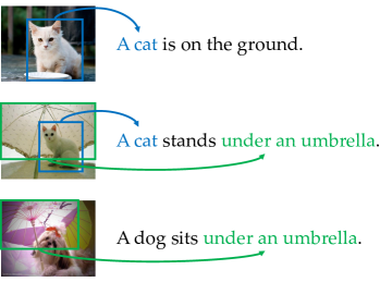
Figure 1: We propose to use image-caption pairs to extract constituents from text, based on the assumption that similar spans should be matched to similar visual objects and these concrete spans form constituents.

1 Introduction

We study the problem of visually grounded syntax acquisition. Consider the images in Figure 1, paired with the descriptive texts (captions) in English. Given no prior knowledge of English, and sufficient such pairs, one can infer the correspondence between certain words and visual attributes, (e.g., recognizing that “a cat” refers to the objects in the blue boxes). One can further extract constituents, by assuming that concrete spans of words should be processed as a whole, and thus form the constituents. Similarly, the same process can be applied to verb or prepositional phrases.

This intuition motivates the use of image-text pairs to facilitate automated language learning, including both syntax and semantics. In this paper we focus on learning syntactic structures, and propose the Visually Grounded Neural Syntax Learner (VG-NSL, shown in Figure 2). VG-NSL acquires syntax, in the form of constituency parsing, by looking at images and reading captions.

At a high level, VG-NSL builds latent constituency trees of word sequences and recursively composes representations for constituents. Next, it matches the visual and textual representations. The training procedure is built on the hypothesis that a better syntactic structure contributes to a better representation of constituents, which then leads to better alignment between vision and language. We use no human-labeled constituency trees or other syntactic labeling (such as part-of-speech tags). Instead, we define a concreteness score of constituents based on their matching with images, and use it to guide the parsing of sentences. At test time, no images paired with the text are needed.

We compare VG-NSL with prior approaches to unsupervised language learning, most of which do not use visual grounding. Our first finding is that VG-NSL improves over the best previous approaches to unsupervised constituency parsing in terms of $\text{F}_{1}$ scores against gold parse trees. We also find that many existing approaches are quite unstable with respect to the choice of random initialization, whereas VG-NSL exhibits consistent parsing results across multiple training runs. Third, we analyze the performance of different models on different types of constituents, and find that our model shows substantial improvement on noun phrases and prepositional phrases which are common in captions. Fourth, VG-NSL is much more data-efficient than prior work based purely on text, achieving comparable performance to other approaches using only 20% of the training captions. In addition, the concreteness score, which emerges during the matching between constituents and images, correlates well with a similar measure defined by linguists. Finally, VG-NSL can be easily extended to multiple languages, which we evaluate on the Multi30K data set Elliott et al. (2016, 2017) consisting of German and French image captions.

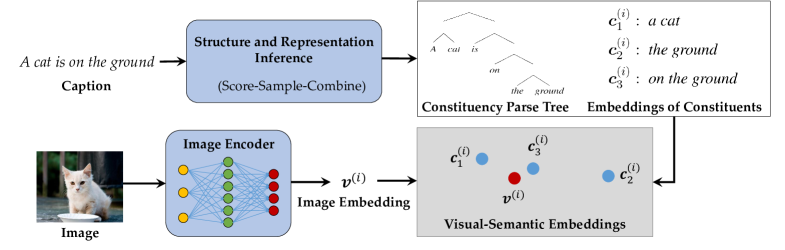
Figure 2: VG-NSL consists of two modules: a textual module for inferring structures and representations for captions, and a visual-semantic module for matching constituents with images. VG-NSL induces constituency parse trees of captions by looking at images and reading paired captions.

2 Related Work

Linguistic structure induction from text.

Recent work has proposed several approaches for inducing latent syntactic structures, including constituency trees (Choi et al., 2018; Yogatama et al., 2017; Maillard and Clark, 2018; Havrylov et al., 2019; Kim et al., 2019; Drozdov et al., 2019) and dependency trees (Shi et al., 2019), from the distant supervision of downstream tasks. However, most of the methods are not able to produce linguistically sound structures, or even consistent ones with fixed data and hyperparameters but different random initializations (Williams et al., 2018).

A related line of research is to induce latent syntactic structure via language modeling. This approach has achieved remarkable performance on unsupervised constituency parsing Shen et al. (2018a, 2019), especially in identifying the boundaries of higher-level (i.e., larger) constituents. To our knowledge, the Parsing-Reading-Predict Network (PRPN; Shen et al., 2018a) and the Ordered Neuron LSTM (ON-LSTM; Shen et al., 2019) currently produce the best fully unsupervised constituency parsing results. One issue with PRPN, however, is that it tends to produce meaningless parses for lower-level (smaller) constituents Phu Mon Htut et al. (2018).

Over the last two decades, there has been extensive study targeting unsupervised constituency parsing (Klein and Manning, 2002, 2004, 2005; Bod, 2006a, b; Ponvert et al., 2011) and dependency parsing (Klein and Manning, 2004; Smith and Eisner, 2006; Spitkovsky et al., 2010; Han et al., 2017). However, all of these approaches are based on linguistic annotations. Specifically, they operate on the part-of-speech tags of words instead of word tokens. One exception is Spitkovsky et al. (2011), which produces dependency parse trees based on automatically induced pseudo tags.

In contrast to these existing approaches, we focus on inducing constituency parse trees with visual grounding. We use parallel data from another modality (i.e., paired images and captions), instead of linguistic annotations such as POS tags. We include a detailed comparison between some related works in the supplementary material.

There has been some prior work on improving unsupervised parsing by leveraging extra signals, such as parallel text (Snyder et al., 2009), annotated data in another language with parallel text (Ganchev et al., 2009), annotated data in other languages without parallel text (Cohen et al., 2011), or non-parallel text from multiple languages (Cohen and Smith, 2009). We leave the integration of other grounding signals as future work.

Grounded language acquisition.

Grounded language acquisition has been studied for image-caption data (Christie et al., 2016a), video-caption data (Siddharth et al., 2014; Yu et al., 2015), and visual reasoning (Mao et al., 2019). However, existing approaches rely on human labels or rules for classifying visual attributes or actions. Instead, our model induces syntax structures with no human-defined labels or rules.

Meanwhile, learning visual-semantic representations in a joint embedding space (Ngiam et al., 2011) is a widely studied approach, and has achieved remarkable results on image-caption retrieval (Kiros et al., 2014; Faghri et al., 2018; Shi et al., 2018a), image caption generation (Kiros et al., 2014; Karpathy and Fei-Fei, 2015; Ma et al., 2015), and visual question answering (Malinowski et al., 2015). In this work, we borrow this idea to match visual and textual representations.

Concreteness estimation.

Turney et al. (2011) define concrete words as those referring to things, events, and properties that we can perceive directly with our senses. Subsequent work has studied word-level concreteness estimation based on text (Turney et al., 2011; Hill et al., 2013), human judgments (Silberer and Lapata, 2012; Hill and Korhonen, 2014a; Brysbaert et al., 2014), and multi-modal data (Hill and Korhonen, 2014b; Hill et al., 2014; Kiela et al., 2014; Young et al., 2014; Hessel et al., 2018; Silberer et al., 2017; Bhaskar et al., 2017). As with Hessel et al. (2018) and Kiela et al. (2014), our model uses multi-modal data to estimate concreteness. Compared with them, we define concreteness for spans instead of words, and use it to induce linguistic structures.

3 Visually Grounded Neural Syntax Learner

Given a set of paired images and captions, our goal is to learn representations and structures for words and constituents. Toward this goal, we propose the Visually Grounded Neural Syntax Learner (VG-NSL), an approach for the grounded acquisition of syntax of natural language. VG-NSL is inspired by the idea of semantic bootstrapping (Pinker, 1984), which suggests that children acquire syntax by first understanding the meaning of words and phrases, and linking them with the syntax of words.

At a high level (Figure 2), VG-NSL consists of 2 modules. First, given an input caption (i.e., a sentence or a smaller constituent), as a sequence of tokens, VG-NSL builds a latent constituency parse tree, and recursively composes representations for every constituent. Next, it matches textual representations with visual inputs, such as the paired image with the constituents. Both modules are jointly optimized from natural supervision: the model acquires constituency structures, composes textual representations, and links them with visual scenes, by looking at images and reading paired captions.

3.1 Textual Representations and Structures

VG-NSL starts by composing a binary constituency structure of text, using an easy-first bottom-up parser Goldberg and Elhadad (2010). The composition of the tree from a caption of length $n$ consists of $n-1$ steps. Let $\mathbf{X}^{(t)}=(\mathbf{x}^{(t)}_{1},\mathbf{x}^{(t)}_{2},\cdots,\mathbf{x}^{(t)}_{k})$ denote the textual representations of a sequence of constituents after step $t$, where $k=n-t$. For simplicity, we use $\mathbf{X}^{(0)}$ to denote the word embeddings for all tokens (the initial representations).

At step $t$, a score function $\textit{score}(\cdot;\Theta)$, parameterized by $\Theta$, is evaluated on all pairs of consecutive constituents, resulting in a vector $\textit{{score}}(\mathbf{X}^{(t-1)};\Theta)$ of length $n-t$:

score $$(\mathbf{X}^{(t-1)};\Theta)_{j}$$

$$\triangleq\textit{score}\left(\left[\mathbf{x}^{(t-1)}_{j},\mathbf{x}^{(t-1)}_{j+1}\right];\Theta\right).$$

We implement $score(\cdot;\Theta)$ as a two-layer feed-forward network.

A pair of constituents $\left(\mathbf{x}^{(t-1)}_{j^{*}},\mathbf{x}^{(t-1)}_{j^{*}+1}\right)$ is sampled from all pairs of consecutive constituents, with respect to the distribution produced by a softmax:

$$\Pr\left[j^{*}\right] =\frac{\exp\left(\textit{score}\left(\mathbf{X}^{(t-1)};\Theta\right)_{j^{*}}\right)}{\sum_{j}\exp\left(\textit{score}\left(\mathbf{X}^{(t-1)};\Theta\right)_{j}\right)}.$$

The selected pair is combined to form a single new constituent. Thus, after step $t$, the number of constituents is decreased by 1. The textual representation for the new constituent is defined as the L2-normed sum of the two component constituents:

$$\textit{combine}\left(\mathbf{x}^{(t-1)}_{j^{*}},\mathbf{x}^{(t-1)}_{j^{*}+1}\right)\triangleq\frac{\mathbf{x}^{(t-1)}_{j^{*}}+\mathbf{x}^{(t-1)}_{j^{*}+1}}{\left\|\mathbf{x}^{(t-1)}_{j^{*}}+\mathbf{x}^{(t-1)}_{j^{*}+1}\right\|_{2}}.$$

We find that using a more complex encoder for constituents, such as GRUs, will cause the representations to be highly biased towards a few salient words in the sentence (e.g., the encoder encodes only the word “cat” while ignoring the rest part of the caption; Shi et al., 2018a; Wu et al., 2019). This significantly degrades the performance of linguistic structure induction.

We repeat this score-sample-combine process for $n-1$ steps, until all words in the input text have been combined into a single constituent (Figure 3). This ends the inference of the constituency parse tree. Since at each time step we combine two consecutive constituents, the derived tree $\mathbf{t}$ contains $2n-1$ constituents (including all words).

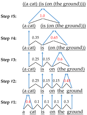
Figure 3: An illustration of how VG-NSL composes a constituency parse tree. At each step, the score function $score$ is evaluated on all pairs of consecutive constituents (dashed lines). Next, a pair of constituents is sampled from all pairs w.r.t. a distribution computed by the softmax of all predicted scores. The selected pair of constituents is combined into a larger one, while the other constituents remain unchanged (solid lines).

3.2 Visual-Semantic Embeddings

We follow an approach similar to that of Kiros et al. (2014) to define the visual-semantic embedding (VSE) space for paired images and text constituents. Let $\mathbf{v}^{(i)}$ denote the vector representation of an image $i$, and $\mathbf{c}^{(i)}_{j}$ denote the vector representation of the $j$-th constituent of its corresponding text caption. During the matching with images, we ignore the tree structure and index them as a list of constituents. A function $m(\cdot,\cdot;\Phi)$ is defined as the matching score between images and texts:

$$m(\mathbf{v}^{(i)},\mathbf{c}^{(i)}_{j};\Phi) \triangleq\cos(\Phi\mathbf{v},\mathbf{c}),$$

where the parameter vector $\Phi$ aligns the visual and textual representations into a joint space.

3.3 Training

We optimize the visual-semantic representations ($\Phi$) and constituency structures ($\Theta$) in an alternating approach. At each iteration, given constituency parsing results of caption, $\Phi$ is optimized for matching the visual and the textual representations. Next, given the visual grounding of constituents, $\Theta$ is optimized for producing constituents that can be better matched with images. Specifically, we optimize textual representations and the visual-semantic embedding space using a hinge-based triplet ranking loss:

$$\begin{aligned} &\mathcal{L}(\Phi;\mathcal{V},\mathcal{C})=\\ &\sum_{\begin{subarray}{c}i,k\neq i,j,\ell\end{subarray}}\left[m(\mathbf{c}^{(k)}_{\ell},\mathbf{v}^{(i)})-m(\mathbf{c}^{(i)}_{j},\mathbf{v}^{(i)})+\delta\right]_{+}\\ +&\sum_{\begin{subarray}{c}i,k\neq i,j\end{subarray}}\left[m(\mathbf{c}^{(i)}_{j},\mathbf{v}^{(k)})-m(\mathbf{c}^{(i)}_{j},\mathbf{v}^{(i)})+\delta\right]_{+},\end{aligned}$$

where $i$ and $k$ index over all image-caption pairs in the data set, while $j$ and $\ell$ enumerate all constituents of a specific caption ($c^{(i)}$ and $c^{(k)}$, respectively), $\mathcal{V}=\{\mathbf{v}^{(i)}\}$ is the set of image representations, $\mathcal{C}=\{\mathbf{c}^{(i)}_{j}\}$ is the set of textual representations of all constituents, and $\delta$ is a constant margin, $[\cdot]_{+}$ denotes $\max(0,\cdot)$. The loss $\mathcal{L}$ extends the loss for image-caption retrieval of Kiros et al. (2014), by introducing the alignments between images and sub-sentence constituents.

We optimize textual structures via distant supervision: they are optimized for a better alignment between the derived constituents and the images. Intuitively, the following objective encourages adjectives to be associated (combined) with the corresponding nouns, and verbs/prepositions to be associated (combined) with the corresponding subjects and objects. Specifically, we use REINFORCE (Williams, 1992) as the gradient estimator for $\Theta$. Consider the parsing process of a specific caption $c^{(i)}$, and denote the corresponding image embedding $\mathbf{v}^{(i)}$. For a constituent $\mathbf{z}$ of $c^{(i)}$, we define its (visual) concreteness $\textit{concrete}(\mathbf{z},\mathbf{v}^{(i)})$ as:

$$\textit{concrete}(\mathbf{z},\mathbf{v}^{(i)})=$$

$$\sum_{k\neq i,p}\left[m(\mathbf{z},\mathbf{v}^{(i)})-m(\mathbf{c}^{(k)}_{p},\mathbf{v}^{(i)})-\delta^{\prime}\right]_{+}$$

$$+ \sum_{k\neq i}\left[m(\mathbf{z},\mathbf{v}^{(i)})-m(\mathbf{z},\mathbf{v}^{(k)})-\delta^{\prime}\right]_{+},$$ (1)

where $\delta^{\prime}$ is a fixed margin. At step $t$, we define the reward function for a combination of a pair of constituents ($\mathbf{x}^{(t-1)}_{j}$, $\mathbf{x}^{(t-1)}_{j+1}$) as:

$$r(\mathbf{x}^{(t-1)}_{j},\mathbf{x}^{(t-1)}_{j+1})=\textit{concrete}(\mathbf{z},\mathbf{v}^{(i)}),$$ (2)

where $\mathbf{z}\triangleq\textit{combine}(\mathbf{x}^{(t-1)}_{j},\mathbf{x}^{(t-1)}_{j+1})$. In plain words, at each step, we encourage the model to compose a constituent that maximizes the alignment between the new constituent and the corresponding image. During training, we sample constituency parse trees of captions, and reinforce each composition step using Equation 2. During test, no paired images of text are needed.

3.4 The Head-Initial Inductive Bias

English and many other Indo-European languages are usually head-initial Baker (2001). For example, in verb phrases or prepositional phrases, the verb (or the preposition) precedes the complements (e.g., the object of the verb). Consider the simple caption a white cat on the lawn. While the association of the adjective (white) could be induced from the visual grounding of phrases, whether the preposition (on) should be associated with a white cat or the lawn is more challenging to induce. Thus, we impose an inductive bias to guide the learner to correctly associate prepositions with their complements, determiners with corresponding noun phrases, and complementizers with the corresponding relative clauses. Specifically, we discourage abstract constituents (i.e., constituents that cannot be grounded in the image) from being combined with a preceding constituent, by modifying the original reward definition (Equation 2) as:

$$r^{\prime}(\mathbf{x}^{(t-1)}_{j}, \mathbf{x}^{(t-1)}_{j+1})$$ (3)

$$= \frac{r(\mathbf{x}^{(t-1)}_{j},\mathbf{x}^{(t-1)}_{j+1})}{\lambda\cdot\textit{abstract}(\mathbf{x}^{(t-1)}_{j+1},\mathbf{v}^{(i)})+1}\ ,$$

where $\lambda$ is a scalar hyperparameter, $\mathbf{v}^{(i)}$ is the image embedding corresponding to the caption being parsed, and $abstract$ denotes the abstractness of the span, defined analogously to concreteness (Equation 1):

$$\textit{abstract}(\mathbf{z},\mathbf{v}^{(i)})=$$

$$\sum_{k\neq i,p}\left[m(\mathbf{c}^{(k)}_{p},\mathbf{v}^{(i)})-m(\mathbf{z},\mathbf{v}^{(i)})+\delta^{\prime}\right]_{+}$$

$$+ \sum_{k\neq i}\left[m(\mathbf{z},\mathbf{v}^{(k)})-m(\mathbf{z},\mathbf{v}^{(i)})+\delta^{\prime}\right]_{+},$$

The intuition here is that the initial heads for prepositional phrases (e.g., on) and relative clauses (e.g., which, where) are usually abstract words. During training, we encourage the model to associate these abstract words with the succeeding constituents instead of the preceding ones. It is worth noting that such an inductive bias is language-specific, and cannot be applied to head-final languages such as Japanese Baker (2001). We leave the design of head-directionality inductive biases for other languages as future work.

4 Experiments

We evaluate VG-NSL for unsupervised parsing in a few ways: $\text{F}_{1}$ score with gold trees, self-consistency across different choices of random initialization, performance on different types of constituents, and data efficiency. In addition, we find that the concreteness score acquired by VG-NSL is consistent with a similar measure defined by linguists. We focus on English for the main experiments, but also extend to German and French.

4.1 Data Sets and Metrics

We use the standard split of the MSCOCO data set Lin et al. (2014), following Karpathy and Fei-Fei (2015). It contains 82,783 images for training, 1,000 for development, and another 1,000 for testing. Each image is associated with 5 captions.

For the evaluation of constituency parsing, the Penn Treebank (PTB; Marcus et al., 1993) is a widely used, manually annotated data set. However, PTB consists of sentences from abstract domains, e.g., the Wall Street Journal (WSJ), which are not visually grounded and whose linguistic structures can hardly be induced by VG-NSL. Here we evaluate models on the MSCOCO test set, which is well-matched to the training domain; we leave the extension of our work to more abstract domains to future work. We apply Benepar Kitaev and Klein (2018), an off-the-shelf constituency parser with state-of-the-art performance (95.52 $\text{F}_{1}$ score) on the WSJ test set, to parse the captions in the MSCOCO test set as gold constituency parse trees. We evaluate all of the investigated models using the $\text{F}_{1}$ score compared to these gold parse trees.

4.2 Baselines

Model	NP		VP		PP		ADJP		Avg. $\textbf{F}_{1}$		Self $\textbf{F}_{1}$
Random	47.3	±0.3	10.5	±0.4	17.3	±0.7	33.5	±0.8	27.1	±0.2	32.4
Left	51.4		1.8		0.2		16.0		$23.3$		N/A
Right	32.2		23.4		18.7		14.4		$22.9$		N/A
PMI	54.2		16.0		14.3		39.2		$30.5$		N/A
PRPN (Shen et al., 2018a)	72.8	±9.7	33.0	±9.1	61.6	±9.9	35.4	±4.3	52.5	±2.6	60.3
ON-LSTM (Shen et al., 2019)	74.4	±7.1	11.8	±5.6	41.3	±16.4	44.0	±14.0	45.5	±3.3	69.3
Gumbel (Choi et al., 2018)†	50.4	±0.3	8.7	±0.3	15.5	±0.0	34.8	±1.6	27.9	±0.2	40.1
VG-NSL (ours)†	79.6	±0.4	26.2	±0.4	42.0	±0.6	22.0	±0.4	50.4	±0.3	87.1
VG-NSL+HI (ours)†	74.6	±0.5	32.5	±1.5	66.5	±1.2	21.7	±1.1	53.3	±0.2	90.2
VG-NSL+HI+FastText (ours)*†	78.8	±0.5	24.4	±0.9	65.6	±1.1	22.0	±0.7	54.4	±0.4	89.8
Concreteness estimation–based models
Turney et al. (2011)*	65.5		30.8		35.3		30.4		42.5		N/A
Turney et al. (2011)+HI*	74.5		26.2		47.6		25.6		48.9		N/A
Brysbaert et al. (2014)*	54.1		27.8		27.0		33.1		34.1		N/A
Brysbaert et al. (2014)+HI*	73.4		23.9		50.0		26.1		47.9		N/A
Hessel et al. (2018)†	50.9		21.7		32.8		27.5		33.2		N/A
Hessel et al. (2018)+HI†	72.5		34.4		65.8		26.2		52.9		N/A

Table 1: Recall of specific typed phrases, and overall $\text{F}_{1}$ score, evaluated on the MSCOCO test split, averaged over 5 runs with different random initializations. We also include self-agreement $\text{F}_{1}$ score Williams et al. (2018) across the 5 runs. $\pm$ denotes standard deviation. * denotes models requiring extra labels and/or corpus, and $\dagger$ denotes models requiring a pre-trained visual feature extractor. We highlight the best number in each column among all models that do not require extra data other than paired image-caption data, as well as the overall best number. The Left, Right, PMI, and concreteness estimation–based models have no standard deviation or self $\text{F}_{1}$ (shown as N/A) as they are deterministic given the training and/or testing data.

We compare VG-NSL with various baselines for unsupervised tree structure modeling of texts. We can categorize the baselines by their training objective or supervision.

Trivial tree structures.

Similarly to recent work on latent tree structures Williams et al. (2018); Phu Mon Htut et al. (2018); Shi et al. (2018b), we include three types of trivial baselines without linguistic information: random binary trees, left-branching binary trees, and right-branching binary trees.

Syntax acquisition by language modeling and statistics.

Shen et al. (2018a) proposes the Parsing-Reading-Predict Network (PRPN), which predicts syntactic distances (Shen et al., 2018b) between adjacent words, and composes a binary tree based on the syntactic distances to improve language modeling. The learned distances can be mapped into a binary constituency parse tree, by recursively splitting the sentence between the two consecutive words with the largest syntactic distance.

Ordered neurons (ON-LSTM; Shen et al., 2019) is a recurrent unit based on the LSTM cell (Hochreiter and Schmidhuber, 1997) that explicitly regularizes different neurons in a cell to represent short-term or long-term information. After being trained on the language modeling task, Shen et al. (2019) suggest that the gate values in ON-LSTM cells can be viewed as syntactic distances Shen et al. (2018b) between adjacent words to induce latent tree structures. ON-LSTM has the state-of-the-art unsupervised constituency parsing performance on the WSJ test set. We train both PRPN and ON-LSTM on all captions in the MSCOCO training set and use the models as baselines.

Inspired by the syntactic distance–based approaches (Shen et al., 2018a, 2019), we also introduce another baseline, PMI, which uses negative pointwise mutual information Church and Hanks (1990) between adjacent words as the syntactic distance. We compose constituency parse trees based on the distances in the same way as PRPN and ON-LSTM.

Syntax acquisition from downstream tasks.

Choi et al. (2018) propose to compose binary constituency parse trees directly from downstream tasks using the Gumbel softmax trick Jang et al. (2017). We integrate a Gumbel tree-based caption encoder into the visual semantic embedding approach Kiros et al. (2014). The model is trained on the downstream task of image-caption retrieval.

Syntax acquisition from concreteness estimation.

Since we apply concreteness information to train VG-NSL, it is worth comparing against unsupervised constituency parsing based on previous approaches for predicting word concreteness. This set of baselines includes semi-supervised estimation Turney et al. (2011), crowdsourced labeling Brysbaert et al. (2014), and multimodal estimation Hessel et al. (2018). Note that none of these approaches has been applied to unsupervised constituency parsing. Implementation details can be found in the supplementary material.

Based on the concreteness score of words, we introduce another baseline similar to VG-NSL. Specifically, we recursively combine two consecutive constituents with the largest average concreteness, and use the average concreteness as the score for the composed constituent. The algorithm generates binary constituency parse trees of captions. For a fair comparison, we implement a variant of this algorithm that also uses a head-initial inductive bias and include the details in the appendix.

4.3 Implementation Details

Across all experiments and all models (including baselines such as PRPN, ON-LSTM, and Gumbel), the embedding dimension for words and constituents is 512. For VG-NSL, we use a pre-trained ResNet-101 (He et al., 2016), trained on ImageNet (Russakovsky et al., 2015), to extract vector embeddings for images. Thus, $\Phi$ is a mapping from a 2048-D image embedding space to a 512-D visual-semantic embedding space. As for the score function in constituency parsing, we use a hidden dimension of 128 and ReLU activation. All VG-NSL models are trained for 30 epochs. We use an Adam optimizer (Kingma and Ba, 2015) with initial learning rate $5\times 10^{-4}$ to train VG-NSL. The learning rate is re-initialized to $5\times 10^{-5}$ after 15 epochs. We tune other hyperparameters of VG-NSL on the development set using the self-agreement $\text{F}_{1}$ score Williams et al. (2018) over 5 runs with different choices of random initialization.

4.4 Results: Unsupervised Constituency Parsing

We evaluate the induced constituency parse trees via the overall $\text{F}_{1}$ score, as well as the recall of four types of constituents: noun phrases (NP), verb phrases (VP), prepositional phrases (PP), and adjective phrases (ADJP) (Table 1). We also evaluate the robustness of models trained with fixed data and hyperparameters, but different random initialization, in two ways: via the standard deviation of performance across multiple runs, and via the self-agreement $\text{F}_{1}$ score Williams et al. (2018), which is the average $\text{F}_{1}$ taken over pairs of different runs.

Among all of the models which do not require extra labels, VG-NSL with the head-initial inductive bias (VG-NSL+HI) achieves the best $\text{F}_{1}$ score. PRPN Shen et al. (2018a) and a concreteness estimation-based baseline (Hessel et al., 2018) both produce competitive results. It is worth noting that the PRPN baseline reaches this performance without any information from images. However, the performance of PRPN is less stable than that of VG-NSL across random initializations. In contrast to its state-of-the-art performance on the WSJ full set (Shen et al., 2019), we observe that ON-LSTM does not perform well on the MSCOCO caption data set. However, it remains the best model for adjective phrases, which is consistent with the result reported by Shen et al. (2019).

In addition to the best overall $\text{F}_{1}$ scores, VG-NSL+HI achieves competitive scores across most phrase types (NP, VP and PP). Our models (VG-NSL and VG-NSL+HI) perform the best on NP and PP, which are the most common visually grounded phrases in the MSCOCO data set. In addition, our models produce much higher self $\text{F}_{1}$ than the baselines Shen et al. (2018a, 2019); Choi et al. (2018), showing that they reliably produce reasonable constituency parse trees with different initialization.

We also test the effectiveness of using pre-trained word embeddings. Specifically, for VG-NSL+HI+FastText, we use a pre-trained FastText embedding (300-D, Joulin et al., 2016), concatenated with a 212-D trainable embedding, as the word embedding. Using pre-trained word embeddings further improves performance to an average $\text{F}_{1}$ of 54.4% while keeping a comparable self $\text{F}_{1}$.

4.5 Results: Data Efficiency

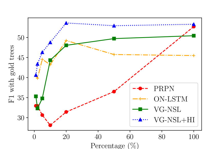
(a) The percent data-$\text{F}_{1}$ curves.

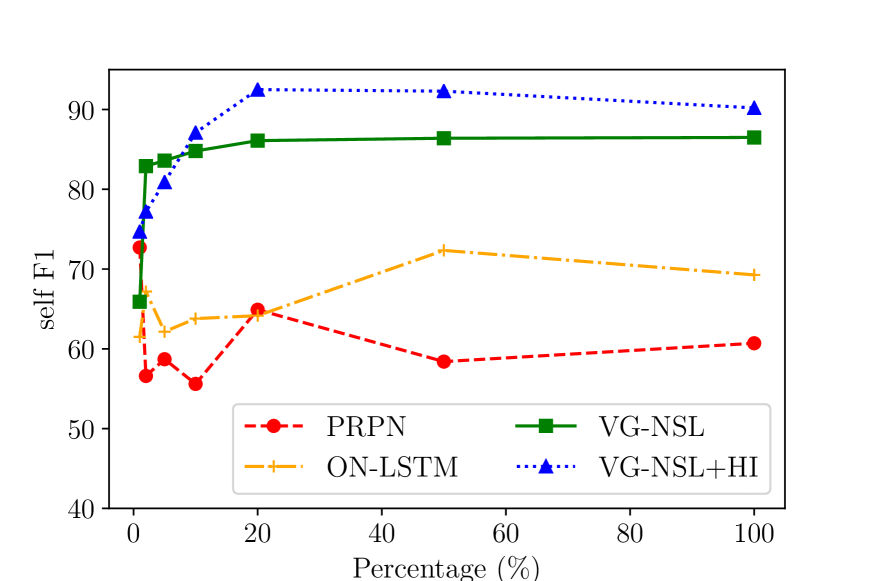
(b) The percent data-self $\text{F}_{1}$ curves.

Figure 4: $\text{F}_{1}$ score and self $\text{F}_{1}$ score with respect to the amount of training data. All numbers are averaged over 5 runs with different random initialization.

We compare the data efficiency for PRPN (the strongest baseline method), ON-LSTM, VG-NSL, and VG-NSL+HI. We train the models using 1%, 2%, 5%, 10%, 20%, 50% and 100% of the MSCOCO training set, and report the overall $\text{F}_{1}$ and self $\text{F}_{1}$ scores on the test set (Figure 4).

Compared to PRPN trained on the full training set, VG-NSL and VG-NSL+HI reach comparable performance using only 20% of the data (i.e., 8K images with 40K captions). VG-NSL tends to quickly become more stable (in terms of the self $\text{F}_{1}$ score) as the amount of data increases, while PRPN and ON-LSTM remain less stable.

4.6 Analysis: Consistency with Linguistic Concreteness

Model/method	VG-NSL	(+HI)
Turney et al. (2011)	0.74	0.72
Brysbaert et al. (2014)	0.71	0.71
Hessel et al. (2018)	0.84	0.85

Table 2: Agreement between our concreteness estimates and existing models or labels, evaluated via the Pearson correlation coefficient computed over the most frequent 100 words in the MSCOCO test set, averaged over 5 runs with different random initialization.

During training, VG-NSL acquires concreteness estimates for constituents via Equation 1. Here, we evaluate the consistency between word-level concreteness estimates induced by VG-NSL and those produced by other methods Turney et al. (2011); Brysbaert et al. (2014); Hessel et al. (2018). Specifically, we measure the correlation between the concreteness estimated by VG-NSL on MSCOCO test set and existing linguistic concreteness definitions (Table 2). For any word, of which the representation is $\mathbf{z}$, we estimate its concreteness by taking the average of $\textit{concrete}(\mathbf{z},\mathbf{v}^{(i)})$, across all associated images $\mathbf{v}^{(i)}$. The high correlation between VG-NSL and the concreteness scores produced by Turney et al. (2011) and Brysbaert et al. (2014) supports the argument that the linguistic concept of concreteness can be acquired in an unsupervised way. Our model also achieves a high correlation with Hessel et al. (2018), which also estimates word concreteness based on visual-domain information.

4.7 Analysis: Self-Agreement $\text{F}_{1}$ Score as the Criterion for Model Selection

Model	Criterion	Avg. $\textbf{F}_{1}$	Self $\textbf{F}_{1}$
VG-NSL	Self $\text{F}_{1}$	50.4 ±0.3	87.1
VG-NSL	R@1	47.7 ±0.6	83.4
VG-NSL+HI	Self $\text{F}_{1}$	53.3 ±0.2	90.2
VG-NSL+HI	R@1	53.1 ±0.2	88.7

Table 3: Average $\text{F}_{1}$ scores and Self $\text{F}_{1}$ scores of VG-NSL and VG-NSL+HI with different model selection methods. R@1 denotes using recall at 1 Kiros et al. (2014) as the model selection criterion. All hyperparameters are tuned with respect to self-agreement $\text{F}_{1}$ score. The numbers are comparable to those in Table 1.

We introduce a novel hyperparameter tuning and model selection method based on the self-agreement $\text{F}_{1}$ score.

Let $\mathcal{M}_{\mathcal{H}}^{(i,j)}$ denote the j-th checkpoint of the i-th model trained with hyperparameters $\mathcal{H}$, where $\mathcal{M}_{\mathcal{H}}^{(i_{1},\cdot)}$ and $\mathcal{M}_{\mathcal{H}}^{(i_{2},\cdot)}$ differ in their random initialization. The hyperparameters $\mathcal{H}$ are tuned to maximize:

$$\sum_{1\leq i<k\leq N} \max_{|j_{i}-j_{k}|<\delta}\textit{F}_{1}\left(\mathcal{M}_{\mathcal{H}}^{(i,j_{i})},\mathcal{M}_{\mathcal{H}}^{(k,j_{k})}\right),$$

where $F_{1}(\cdot,\cdot)$ denotes the $\text{F}_{1}$ score between the trees generated by two models, $N$ the number of different runs, and $\delta$ the margin to ensure only nearby checkpoints are compared.

After finding the best hyperparameters $\mathcal{H}_{0}$, we train the model for another $N$ times with different random initialization, and select the best models by

$$\operatorname*{arg\,max}_{\{j_{\ell}\}_{\ell=1}^{N}}\sum_{1\leq i<k\leq N}\textit{F}_{1}\left(\mathcal{M}_{\mathcal{H}_{0}}^{(i,j_{i})},\mathcal{M}_{\mathcal{H}_{0}}^{(k,j_{k})}\right).$$

We compare the performance of VG-NSL selected by the self $\text{F}_{1}$ score and that selected by recall at 1 in image-to-text retrieval (R@1 in Table 3; Kiros et al., 2014). As a model selection criterion, self $\text{F}_{1}$ consistently outperforms R@1 (avg. $\text{F}_{1}$: 50.4 vs. 47.7 and 53.3 vs. 53.1 for VG-NSL and VG-NSL+HI, respectively). Meanwhile, it is worth noting that even if we select VG-NSL by R@1, it shows better stability compared with PRPN and ON-LSTM (Table 1), in terms of the score variance across different random initialization and self $\text{F}_{1}$. Specifically, the variance of avg. $\text{F}_{1}$ is always less than 0.6 while the self $\text{F}_{1}$ is greater than 80.

Note that the PRPN and ON-LSTM models are not tuned using self $\text{F}_{1}$, since these models are usually trained for hundreds or thousands of epochs and thus it is computationally expensive to evaluate self $\text{F}_{1}$. We leave the efficient tuning of these baselines by self $\text{F}_{1}$ as a future work.

4.8 Extension to Multiple Languages

Model	EN		DE		FR
PRPN	30.8	±17.9	31.5	±8.9	27.5	±7.0
ON-LSTM	38.7	±12.7	34.9	±12.3	27.7	±5.6
VG-NSL	33.5	±0.2	36.3	±0.2	34.3	±0.6
VG-NSL+HI	38.7	±0.2	38.3	±0.2	38.1	±0.6

Table 4: $\text{F}_{1}$ scores on the Multi30K test split Young et al. (2014); Elliott et al. (2016, 2017), averaged over 5 runs with different random initialization. $\pm$ denotes the standard deviation.

We extend our experiments to the Multi30K data set, which is built on the Flickr30K data set Young et al. (2014) and consists of English, German Elliott et al. (2016), and French Elliott et al. (2017) captions. For Multi30K, there are 29,000 images in the training set, 1,014 in the development set and 1,000 in the test set. Each image is associated with one caption in each language.

We compare our models to PRPN and ON-LSTM in terms of overall $\text{F}_{1}$ score (Table 4). VG-NSL with the head-initial inductive bias consistently performs the best across the three languages, all of which are highly head-initial Baker (2001). Note that the $\text{F}_{1}$ scores here are not comparable to those in Table 1, since Multi30K (English) has 13x fewer captions than MSCOCO.

5 Discussion

We have proposed a simple but effective model, the Visually Grounded Neural Syntax Learner, for visually grounded language structure acquisition. VG-NSL jointly learns parse trees and visually grounded textual representations. In our experiments, we find that this approach to grounded language learning produces parsing models that are both accurate and stable, and that the learning is much more data-efficient than a state-of-the-art text-only approach. Along the way, the model acquires estimates of word concreteness.

The results suggest multiple future research directions. First, VG-NSL matches text embeddings directly with embeddings of entire images. Its performance may be boosted by considering structured representations of both images (e.g., Lu et al., 2016; Wu et al., 2019) and texts (Steedman, 2000). Second, thus far we have used a shared representation for both syntax and semantics, but it may be useful to disentangle their representations (Steedman, 2000). Third, our best model is based on the head-initial inductive bias. Automatically acquiring such inductive biases from data remains challenging (Kemp et al., 2006; Gauthier et al., 2018). Finally, it may be possible to extend our approach to other linguistic tasks such as dependency parsing (Christie et al., 2016b), coreference resolution (Kottur et al., 2018), and learning pragmatics beyond semantics (Andreas and Klein, 2016).

There are also limitations to the idea of grounded language acquisition. In particular, the current approach has thus far been applied to understanding grounded texts in a single domain (static visual scenes for VG-NSL). Its applicability could be extended by learning shared representations across multiple modalities (Castrejon et al., 2016) or integrating with pure text-domain models (such as PRPN, Shen et al., 2018a).

Supplementary Material
The supplementary material is organized as follows. First, in Section A, we summarize and compare existing models for constituency parsing without explicit syntactic supervision. Next, in Section B, we present more implementation details of VG-NSL. Third, in Section C, we present the implementation details for all of our baseline models. Fourth, in Section D, we present the evaluation details of Benepar Kitaev and Klein (2018) on the MSCOCO data set. Fifth, in Section E, we qualitatively and quantitatively compare the concreteness scores estimated or labeled by different methods. Finally, in Section F, we show sample trees generated by VG-NSL on the MSCOCO test set.

Appendix A Overview of Models for Constituency Parsing without Explicit Syntactic Supervision

Model	Objective	Extra Label	Multi-	Stochastic	Extra
			modal		Corpus
CCM Klein and Manning (2002)*	MAP	POS	✗	✓	✗
DMV-CCM Klein and Manning (2005)*	MAP	POS	✗	✓	✗
U-DOP Bod (2006b)*	Probability Estimation	POS	✗	✗	✗
UML-DOP Bod (2006a)*	MAP	POS	✗	✓	✗
PMI	N/A	✗	✗	✗	✗
Random	N/A	✗	✗	✓	✗
Left	N/A	✗	✗	✗	✗
Right	N/A	✗	✗	✗	✗
PRPN Shen et al. (2018a)	LM	✗	✗	✓	✗
ON-LSTM Shen et al. (2019)	LM	✗	✗	✓	✗
Gumbel softmaxChoi et al. (2018)	Cross-modal Retrieval	✗	✓	✓	✗
VG-NSL (ours)	Cross-modal Retrieval	✗	✓	✓	✗
VG-NSL+HI (ours)	Cross-modal Retrieval	✗	✓	✓	✗
Concreteness estimation based models
Turney et al. (2011)*	N/A	Concreteness (Partial)	✗	✗	✓
Turney et al. (2011)+HI*	N/A	Concreteness (Partial)	✗	✗	✓
Brysbaert et al. (2014)*	N/A	Concreteness (Full)	✗	✗	✗
Brysbaert et al. (2014)+HI*	N/A	Concreteness (Full)	✗	✗	✗
Hessel et al. (2018)	N/A	✗	✓	✗	✗
Hessel et al. (2018)+HI	N/A	✗	✓	✗	✗

Table 5: Comparison of models for constituency parsing without explicit syntactic supervision. * denotes models requiring extra labels, such as POS tags or manually labeled concreteness scores. All multimodal methods listed in the table require a pretrained visual feature extractor (i.e., ResNet-101; He et al., 2016). A model is labeled as stochastic if for fixed training data and hyperparameters the model may produce different results (e.g., due to different choices of random initialization). To the best of our knowledge, results on concreteness estimation Turney et al. (2011); Brysbaert et al. (2014); Hessel et al. (2018) have not been applied to unsupervised parsing so far.

Acat is on the ground

(a) Left-branching tree.

A cat is on theground

(b) Right-branching tree.

Figure 5: Examples of some trivial tree structures.

Shown in Table 5, we compare existing models for constituency parsing without explicit syntactic supervision, with respect to their learning objective, dependence on extra labels or extra corpus, and other features. The table also includes the analysis of previous works on parsing sentences based on gold part-of-speech tags.

Appendix B Implementation Details for VG-NSL

We adopt the code released by Faghri et al. (2018) as the visual-semantic embedding module for VG-NSL. Following them, we fix the margin $\delta$ to $0.2$. We also use the vocabulary provided by Faghri et al. (2018), which contains 10,000 frequent words in the MSCOCO data set. Out-of-vocabulary words are treated as unseen words. For either VG-NSL or baselines, we use the same vocabulary if applicable.

Hyperparameter tuning.

As stated in main text, we use the self-agreement $\text{F}_{1}$ score Williams et al. (2018) as an unsupervised signal for tuning all hyperparamters. Besides the learning rate and other conventional hyperparameters, we also tune $\lambda$, the hyperparameter for the head-initial bias model. $\lambda$ indicates the weight of penalization for “right abstract constituents”. We choose $\lambda$ from $\{1,2,5,10,20,50,100\}$ and found that $\lambda=20$ gives the best self-agreement $\text{F}_{1}$ score.

Appendix C Implementation Details for Baselines

Trivial tree structures.

We show examples for left-branching binary trees and right-branching binary trees in Figure 5. As for binary random trees, we iteratively combine two randomly selected adjacent constituents. This procedure is similar to that shown in Algorithm 2.

Parsing-Reading-Predict Network (PRPN).

We use the code released by Shen et al. (2018a) to train PRPN. We tune the hyperparameters with respect to language modeling perplexity Jelinek et al. (1977). For a fair comparison, we fix the hidden dimension of all hidden layers of PRPN as 512. We use an Adam optimizer Kingma and Ba (2015) to optimize the parameters. The tuned parameters are number of layers (1, 2, 3) and learning rate ($1\times 10^{-3}$, $5\times 10^{-4}$, $2\times 10^{-4}$). The models are trained for 100 epochs on the MSCOCO dataset and 1,000 epochs on the Multi30K dataset, and are early stopped using the criterion of language model perplexity.

Ordered Neurons (ON-LSTM).

We use the code release by Shen et al. (2019) to train ON-LSTM. We tune the hyperparameters with respect to language modeling perplexity Jelinek et al. (1977), and use perplexity as an early stopping criterion. For a fair comparison, the hidden dimension of all hidden layers is set to 512, and the chunk size is changed to 16 to fit the hidden layer size. Following the original paper (Shen et al., 2019), we set the number of layers to be 3, and report the constituency parse tree with respect to the gate values output by the second layer of ON-LSTM. In order to obtain a better perplexity, we explore both Adam Kingma and Ba (2015) and SGD as the optimizer. We tune the learning rate ($1\times 10^{-3}$, $5\times 10^{-4}$, $2\times 10^{-4}$ for Adam, and $0.1$, $1$, $10$, $30$ for SGD). The models are trained for 100 epochs on the MSCOCO dataset and 1,000 epochs on the Multi30K dataset, and are early stopped using the criterion of language model perplexity.

PMI based constituency parsing.

We estimate the pointwise mutual information (PMI; Church and Hanks, 1990) between two words using all captions in MSCOCO training set. We apply negative PMI as syntactic distance Shen et al. (2018b) to generate a binary constituency parse tree recursively. The method of constituency parsing with a given list of syntactic distances is shown in Algorithm 1.

Input: text length $m$, list of syntactic distances $\bm{d}=(d_{1},d_{2},\ldots,d_{m-1})$

Output: Boundaries of constituents $B=\{(L_{i},R_{i})\}_{i=1,\ldots,m-1}$

$B$ = parse($\bm{d}$, $1$, $m$)

 

Function parse($\bm{d}$, left, right)

if $\textit{left}=\textit{right}$ then

       return EmptySet

end if

$p=\operatorname*{arg\,max}_{j\in[\textit{left},\textit{right-1}]}d_{j}$

$\textit{boundaries}=$ union(

   {(left, right)},

  parse ($\bm{d}$, left, $p$),

  parse ($\bm{d}$, $p+1$, right)

)

return boundaries

Algorithm 1 Constituency parsing based on given syntactic distance.

Gumbel-softmax based latent tree.

We integrate Gumbel-softmax latent tree based text encoder Choi et al. (2018) to the visual semantic embedding framework Faghri et al. (2018), and use the tree structure produced by it as a baseline.

	Turney et al. (2011)	Brysbaert et al. (2014)	Hessel et al. (2018)	VG-NSL+HI
Turney et al. (2011)	1.00	0.84	0.58	0.72
Brysbaert et al. (2014)	0.84	1.00	0.55	0.71
Hessel et al. (2018)	0.58	0.55	1.00	0.85
VG-NSL+HI	0.72	0.71	0.85	1.00

Table 6: Pearson correlation coefficients between existing concreteness estimation methods, including baselines and VG-NSL+HI. In order to make a fair comparison, the correlation coefficients are evaluated on the 100 most frequent words on MSCOCO test set.

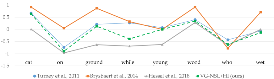
Figure 6: Normalized concreteness scores of example words.

Concreteness estimation.

For the semi-supervised concreteness estimation, we reproduce the experiments by Turney et al. (2011), applying the manually labeled concreteness scores for 4,295 words from the MRC Psycholinguistic Database Machine Usable Dictionary Coltheart (1981) as supervision, and use English Wikipedia pages to estimate PMI between words. The PMI is then used to compute similarity between seen and unseen words, which is further used as weights to estimate concreteness for unseen words. For the concreteness scores from crowdsourcing, we use the released data set of Brysbaert et al. (2014). Similarly to VG-NSL, the multimodal concreteness score Hessel et al. (2018) is also estimated on the MSCOCO training set, using an open-sourced implementation.

Constituency parsing with concreteness scores.

Denote $\alpha(w)$ as the concreteness score estimated by a model for the word $w$. Given a sequence of concreteness scores of caption tokens denoted by $(\alpha(w_{1}),\alpha(w_{2}),\ldots,\alpha(w_{m}))$, we aim to produce a binary constituency parse tree. We first normalize the concreteness scores to the range of $[-1,1]$, via:

$$\alpha^{\prime}(w_{i})=\frac{2\left(\alpha(w_{i})-\frac{\max_{j}\alpha(w_{j})-\min_{j}\alpha(w_{j})}{2}\right)}{\max_{j}\alpha(w_{j})-\min_{j}\alpha(w_{j})}~{}.$$

We treat unseen words (i.e., out-of-vocabulary words) in the same way in VG-NSL, by assigning the concreteness of $-1$ to unseen words, with the assumption that unseen words are the most abstract ones.

We compose constituency parse trees using the normalized concreteness scores by iteratively combining consecutive constituents. At each step, we select two adjacent constituents (initially, words) with the highest average concreteness score and combine them into a larger constituent, of which the concreteness is the average of its children. We repeat the above procedure until there is only one constituent left.

As for the head-initial inductive bias, we weight the concreteness of the right constituent with a hyperparemeter $\tau>1$ when ranking all pairs of consecutive constituents during selection. Meanwhile, the concreteness of the composed constituent remains the average of the two component constituents. In order to keep consistent with VG-NSL, we set $\tau=20$ in all of our experiments.

The procedure is summarized in Algorithm 2.

Input: list of normalized concreteness scores $\bm{a}=(a_{1},a_{2},\ldots,a_{m})$, hyperparameter $\tau$

Output: Boundaries of constituents $B=\{(L_{i},R_{i})\}_{i=1,\ldots,m-1}$

for $j=1$ to $m$ do

       $\textit{left}_{j}=j$

       $\textit{right}_{j}=j$

end for

while $\textit{len}(\bm{a})>1$ do

       $p=\operatorname*{arg\,max}_{j}a_{j}+\tau a_{j+1}$

       add $(\textit{left}_{p},\textit{right}_{p+1})$ to $B$

       $\bm{a}=\bm{a}_{<p}$ + ($\frac{a_{p}+a_{p+1}}{2}$) + $\bm{a}_{>p+1}$

       $\textbf{{left}}=\textbf{{left}}_{<p}$ + ($\textit{left}_{p}$) + $\textbf{{left}}_{>p+1}$

       $\textbf{{right}}=\textbf{{right}}_{<p}$ + ($\textit{right}_{p+1}$) + $\textbf{{right}}_{>p+1}$

end while

Algorithm 2 Constituency parsing based on concreteness estimation.

Threewhitesinks in abathroom under mirrors

(a) Constituency parse tree labeled by Benepar Kitaev and Klein (2018).

Threewhitesinks in abathroom undermirrors

(b) Manually labeled constituency parse tree.

Figure 7: A failure example by Benepar, where it fails to parse the noun phrase “three white sinks in a bathroom under mirrors” – according to human commonsense, it is much more common for sinks, rather than a bathroom, to be under mirrors. However, most of the constituents (e.g., “three white sinks” and “under mirrors”) are still successfully extracted by Benepar.

Appendix D Details of Manual Ground Truth Evaluation

It is important to confirm that the constituency parse trees of the MSCOCO captions produced by Benepar Kitaev and Klein (2018) are of high enough qualities, so that they can serve as reliable ground truth for further evaluation of other models. To verify this, we randomly sample 50 captions from the MSCOCO test split, and manually label the constituency parse trees without reference to either Benepar or the paired images, following the principles by Bies et al. (1995) as much as possible. Note that we only label the tree structures without constituency labels (e.g., NP and PP). Most failure cases by Benepar are related to human commonsense in resolving parsing ambiguities, e.g., prepositional phrase attachments (Figure 7).

We compare the manually labeled trees and those produced by Benepar Kitaev and Klein (2018), and find that the $\text{F}_{1}$ score between them are 95.65.

Appendix E Concreteness by Different Models

E.1 Correlation between Different Concreteness Estimations

We report the correlation of different methods for concreteness estimation, shown in (Table 6). The concreteness given by Turney et al. (2011) and Brysbaert et al. (2014) highly correlate with each other. The concreteness scores estimated on multi-modal dataset (Hessel et al., 2018) also moderately correlates with the aforementioned two methods (Turney et al., 2011; Brysbaert et al., 2014). Compared to the concreteness estimated by Hessel et al. (2018), the one estimated by our model has a stronger correlation with the scores estimated from linguistic data Turney et al. (2011); Brysbaert et al. (2014).

E.2 Concreteness Scores of Sample Words by Different Methods

We present the concreteness scores estimated or labeled by different methods in Figure 6, which qualitatively shows that different methods correlate with others well.

Appendix F Sample Trees Generated by VG-NSL

Figure 8 shows the sample trees generated by VG-NSL with the head-initial inductive bias (VG-NSL+HI). All captions are chosen from the MSCOCO test set.

akitchen with twowindows and two metalsinks

(a) a kitchen with two windows and two metal sinks

a blue smallplane standing at theairstrip

(b) a blue small plane standing at the airstrip

youngboy sitting on top of abriefcase

(c) young boy sitting on top of a briefcase

a smalldog eating aplate ofbroccoli

(d) a small dog eating a plate of broccoli

abuilding with a bunch ofpeople standingaround it

(e) a building with a bunch of people standing around it

ahorse walking by atree in thewoods

(f) a horse walking by a tree in the woods

the goldenwaffle has abanana init

(g) the golden waffle has a banana in it .

abowl full oforanges that still havestems

(h) a bowl full of oranges that still have stems

there is aperson that is sitting in theboat on thewater

(i) there is a person that is sitting in the boat on the water

asandwich andsoup sit on atable

(j) a sandwich and soup sit on a table

a bigumbrella sitting on thebeach

(k) a big umbrella sitting on the beach

Figure 8: Examples of parsing trees generated by VG-NSL.

References

- Andreas and Klein (2016) Jacob Andreas and Dan Klein. 2016. Reasoning about pragmatics with neural listeners and speakers. In Proc. of EMNLP.
- Baker (2001) Mark C. Baker. 2001. The Atoms of Language: The Mind’s Hidden Rules of Grammar. Basic books.
- Bhaskar et al. (2017) Sai Abishek Bhaskar, Maximilian Köper, Sabine Schulte Im Walde, and Diego Frassinelli. 2017. Exploring multi-modal text+image models to distinguish between abstract and concrete nouns. In Proc. of the IWCS workshop on Foundations of Situated and Multimodal Communication.
- Bies et al. (1995) Ann Bies, Mark Ferguson, Karen Katz, Robert MacIntyre, Victoria Tredinnick, Grace Kim, Mary Ann Marcinkiewicz, and Britta Schasberger. 1995. Bracketing guidelines for treebank II style Penn treebank project. University of Pennsylvania, 97.
- Bod (2006a) Rens Bod. 2006a. An all-subtrees approach to unsupervised parsing. In Proc. of COLING-ACL.
- Bod (2006b) Rens Bod. 2006b. Unsupervised parsing with U-DOP. In Proc. of CoNLL.
- Brysbaert et al. (2014) Marc Brysbaert, Amy Beth Warriner, and Victor Kuperman. 2014. Concreteness ratings for 40 thousand generally known English word lemmas. Behav. Res. Methods, 46(3):904–911.
- Castrejon et al. (2016) Lluis Castrejon, Yusuf Aytar, Carl Vondrick, Hamed Pirsiavash, and Antonio Torralba. 2016. Learning aligned cross-modal representations from weakly aligned data. In Proc. of CVPR.
- Choi et al. (2018) Jihun Choi, Kang Min Yoo, and Sang-goo Lee. 2018. Learning to compose task-specific tree structures. In Proc. of AAAI.
- Christie et al. (2016a) Gordon Christie, Ankit Laddha, Aishwarya Agrawal, Stanislaw Antol, Yash Goyal, Kevin Kochersberger, and Dhruv Batra. 2016a. Resolving language and vision ambiguities together: Joint segmentation & prepositional attachment resolution in captioned scenes. In Proc. of EMNLP.
- Christie et al. (2016b) Gordon Christie, Ankit Laddha, Aishwarya Agrawal, Stanislaw Antol, Yash Goyal, Kevin Kochersberger, and Dhruv Batra. 2016b. Resolving language and vision ambiguities together: Joint segmentation & prepositional attachment resolution in captioned scenes. In Proc. of EMNLP.
- Church and Hanks (1990) Kenneth Ward Church and Patrick Hanks. 1990. Word association norms, mutual information, and lexicography. Comput. Linguist., 16(1):22–29.
- Cohen and Smith (2009) Shay Cohen and Noah A. Smith. 2009. Shared logistic normal distributions for soft parameter tying in unsupervised grammar induction. In Proc. of NAACL-HLT.
- Cohen et al. (2011) Shay B. Cohen, Dipanjan Das, and Noah A. Smith. 2011. Unsupervised structure prediction with non-parallel multilingual guidance. In Proc. of EMNLP.
- Coltheart (1981) Max Coltheart. 1981. The MRC psycholinguistic database. Q. J. Exp. Psychol., 33(4):497–505.
- Drozdov et al. (2019) Andrew Drozdov, Pat Verga, Mohit Yadav, Mohit Iyyer, and Andrew McCallum. 2019. Unsupervised latent tree induction with deep inside-outside recursive autoencoders. In Proc. of NAACL-HLT.
- Elliott et al. (2017) Desmond Elliott, Stella Frank, Loïc Barrault, Fethi Bougares, and Lucia Specia. 2017. Findings of the second shared task on multimodal machine translation and multilingual image description. In Proc. of WMT.
- Elliott et al. (2016) Desmond Elliott, Stella Frank, Khalil Sima’an, and Lucia Specia. 2016. Multi30K: Multilingual English-German image descriptions. In Proc. of the 5th Workshop on Vision and Language.
- Faghri et al. (2018) Fartash Faghri, David J. Fleet, Jamie Ryan Kiros, and Sanja Fidler. 2018. VSE++: Improving visual-semantic embeddings with hard negatives. In Proc. of BMVC.
- Ganchev et al. (2009) Kuzman Ganchev, Jennifer Gillenwater, and Ben Taskar. 2009. Dependency grammar induction via bitext projection constraints. In Proc. of ACL-IJCNLP.
- Gauthier et al. (2018) Jon Gauthier, Roger Levy, and Joshua B. Tenenbaum. 2018. Word learning and the acquisition of syntactic–semantic overhypotheses. In Proc. of CogSci.
- Goldberg and Elhadad (2010) Yoav Goldberg and Michael Elhadad. 2010. An efficient algorithm for easy-first non-directional dependency parsing. In Proc. of NAACL-HLT.
- Han et al. (2017) Wenjuan Han, Yong Jiang, and Kewei Tu. 2017. Dependency grammar induction with neural lexicalization and big training data. In Proc. of EMNLP.
- Havrylov et al. (2019) Serhii Havrylov, Germán Kruszewski, and Armand Joulin. 2019. Cooperative learning of disjoint syntax and semantics. In Proc. of NAACL-HLT.
- He et al. (2016) Kaiming He, Xiangyu Zhang, Shaoqing Ren, and Jian Sun. 2016. Deep residual learning for image recognition. In Proc. of CVPR.
- Hessel et al. (2018) Jack Hessel, David Mimno, and Lillian Lee. 2018. Quantifying the visual concreteness of words and topics in multimodal datasets. In Proc. of NAACL-HLT.
- Hill et al. (2013) Felix Hill, Douwe Kiela, and Anna Korhonen. 2013. Concreteness and corpora: A theoretical and practical study. In Proc. of CMCL.
- Hill and Korhonen (2014a) Felix Hill and Anna Korhonen. 2014a. Concreteness and subjectivity as dimensions of lexical meaning. In Proc. of ACL.
- Hill and Korhonen (2014b) Felix Hill and Anna Korhonen. 2014b. Learning abstract concept embeddings from multi-modal data: Since you probably can’t see what i mean. In Proc. of EMNLP.
- Hill et al. (2014) Felix Hill, Roi Reichart, and Anna Korhonen. 2014. Multi-modal models for concrete and abstract concept meaning. TACL, 2(1):285–296.
- Hochreiter and Schmidhuber (1997) Sepp Hochreiter and Jürgen Schmidhuber. 1997. Long short-term memory. Neural Comput., 9(8):1735–1780.
- Jang et al. (2017) Eric Jang, Shixiang Gu, and Ben Poole. 2017. Categorical reparameterization with Gumbel-softmax. In Proc. of ICLR.
- Jelinek et al. (1977) Fred Jelinek, Robert L Mercer, Lalit R Bahl, and James K Baker. 1977. Perplexity—a measure of the difficulty of speech recognition tasks. The Journal of the Acoustical Society of America, 62(S1):S63–S63.
- Joulin et al. (2016) Armand Joulin, Edouard Grave, Piotr Bojanowski, Matthijs Douze, Hérve Jégou, and Tomas Mikolov. 2016. FastText.zip: Compressing text classification models. arXiv preprint arXiv:1612.03651.
- Karpathy and Fei-Fei (2015) Andrej Karpathy and Li Fei-Fei. 2015. Deep visual-semantic alignments for generating image descriptions. In Proc. of CVPR.
- Kemp et al. (2006) Charles K. Kemp, Amy Perfors, and Joshua B. Tenenbaum. 2006. Learning overhypotheses. In Proc. of CogSci.
- Kiela et al. (2014) Douwe Kiela, Felix Hill, Anna Korhonen, and Stephen Clark. 2014. Improving multi-modal representations using image dispersion: Why less is sometimes more. In Proc. of ACL.
- Kim et al. (2019) Yoon Kim, Alexander M Rush, Lei Yu, Adhiguna Kuncoro, Chris Dyer, and Gábor Melis. 2019. Unsupervised recurrent neural network grammars. In Proc. of NAACL-HLT.
- Kingma and Ba (2015) Diederik P. Kingma and Jimmy Ba. 2015. Adam: A method for stochastic optimization. In Proc. of ICLR.
- Kiros et al. (2014) Ryan Kiros, Ruslan Salakhutdinov, and Richard S. Zemel. 2014. Unifying visual-semantic embeddings with multimodal neural language models. arXiv:1411.2539.
- Kitaev and Klein (2018) Nikita Kitaev and Dan Klein. 2018. Constituency parsing with a self-attentive encoder. In Proc. of ACL.
- Klein and Manning (2002) Dan Klein and Christopher D. Manning. 2002. A generative constituent-context model for improved grammar induction. In Proc. of ACL.
- Klein and Manning (2004) Dan Klein and Christopher D. Manning. 2004. Corpus-based induction of syntactic structure: Models of dependency and constituency. In Proc. of ACL.
- Klein and Manning (2005) Dan Klein and Christopher D. Manning. 2005. Natural language grammar induction with a generative constituent-context model. Pattern Recognition, 38(9):1407–1419.
- Kottur et al. (2018) Satwik Kottur, José MF Moura, Devi Parikh, Dhruv Batra, and Marcus Rohrbach. 2018. Visual coreference resolution in visual dialog using neural module networks. In Proc. of ECCV.
- Lin et al. (2014) Tsung-Yi Lin, Michael Maire, Serge Belongie, James Hays, Pietro Perona, Deva Ramanan, Piotr Dollár, and C. Lawrence Zitnick. 2014. Microsoft COCO: Common objects in context. In Proc. of ECCV.
- Lu et al. (2016) Cewu Lu, Ranjay Krishna, Michael Bernstein, and Li Fei-Fei. 2016. Visual relationship detection with language priors. In Proc. of ECCV.
- Ma et al. (2015) Lin Ma, Zhengdong Lu, Lifeng Shang, and Hang Li. 2015. Multimodal convolutional neural networks for matching image and sentence. In Proc. of CVPR.
- Maillard and Clark (2018) Jean Maillard and Stephen Clark. 2018. Latent tree learning with differentiable parsers: Shift-reduce rarsing and chart parsing. In Proc. of the Workshop on the Relevance of Linguistic Structure in Neural Architectures for NLP.
- Malinowski et al. (2015) Mateusz Malinowski, Marcus Rohrbach, and Mario Fritz. 2015. Ask your neurons: A neural-based approach to answering questions about images. In Proc. of ICCV.
- Mao et al. (2019) Jiayuan Mao, Chuang Gan, Pushmeet Kohli, Joshua B Tenenbaum, and Jiajun Wu. 2019. The neuro-symbolic concept learner: Interpreting scenes, words, and sentences from natural supervision. In Proc. of ICLR.
- Marcus et al. (1993) Mitchell Marcus, Beatrice Santorini, and Mary Ann Marcinkiewicz. 1993. Building a large annotated corpus of English: The Penn treebank. Comput. Linguist., 19(2).
- Ngiam et al. (2011) Jiquan Ngiam, Aditya Khosla, Mingyu Kim, Juhan Nam, Honglak Lee, and Andrew Y. Ng. 2011. Multimodal deep learning. In Proc. of ICML.
- Phu Mon Htut et al. (2018) Phu Mon Htut, Kyunghyun Cho, and Samuel R. Bowman. 2018. Grammar induction with neural language models: An unsual replication. In Proc. of EMNLP.
- Pinker (1984) Steven Pinker. 1984. Language Learnability and Language Development. Cambridge University Press.
- Ponvert et al. (2011) Elias Ponvert, Jason Baldridge, and Katrin Erk. 2011. Simple unsupervised grammar induction from raw rext with cascaded finite state models. In Proc. of ACL.
- Russakovsky et al. (2015) Olga Russakovsky, Jia Deng, Hao Su, Jonathan Krause, Sanjeev Satheesh, Sean Ma, Zhiheng Huang, Andrej Karpathy, Aditya Khosla, Michael Bernstein, Alexander C. Berg, and Li Fei-Fei. 2015. ImageNet large scale visual recognition challenge. IJCV, 115(3):211–252.
- Sekine and Collins (1997) Satoshi Sekine and Michael Collins. 1997. Evalb bracket scoring program.
- Shen et al. (2018a) Yikang Shen, Zhouhan Lin, Chin-Wei Huang, and Aaron Courville. 2018a. Neural language modeling by jointly learning syntax and lexicon. In Proc. of ICLR.
- Shen et al. (2018b) Yikang Shen, Zhouhan Lin, Athul Paul Jacob, Alessandro Sordoni, Aaron Courville, and Yoshua Bengio. 2018b. Straight to the tree: Constituency parsing with neural syntactic distance. In Proc. of ACL.
- Shen et al. (2019) Yikang Shen, Shawn Tan, Alessandro Sordoni, and Aaron Courville. 2019. Ordered neurons: Integrating tree structures into recurrent neural networks. In Proc. of ICLR.
- Shi et al. (2018a) Haoyue Shi, Jiayuan Mao, Tete Xiao, Yuning Jiang, and Jian Sun. 2018a. Learning visually-grounded semantics from contrastive adversarial samples. In Proc. of COLING.
- Shi et al. (2018b) Haoyue Shi, Hao Zhou, Jiaze Chen, and Lei Li. 2018b. On tree-based neural sentence modeling. In Proc. of EMNLP.
- Shi et al. (2019) Jiaxin Shi, Lei Hou, Juanzi Li, Zhiyuan Liu, and Hanwang Zhang. 2019. Learning to embed sentences using attentive recursive trees. In Proc. of AAAI.
- Siddharth et al. (2014) N. Siddharth, Andrei Barbu, and Jeffrey Mark Siskind. 2014. Seeing what you’re told: Sentence-guided activity recognition in video. In Proc. of CVPR.
- Silberer et al. (2017) Carina Silberer, Vittorio Ferrari, and Mirella Lapata. 2017. Visually grounded meaning representations. TPAMI, 39(11):2284–2297.
- Silberer and Lapata (2012) Carina Silberer and Mirella Lapata. 2012. Grounded models of semantic representation. In Proc. of EMNLP-CoNLL.
- Smith and Eisner (2006) Noah A. Smith and Jason Eisner. 2006. Annealing structural bias in multilingual weighted grammar induction. In Proc. of COLING-ACL.
- Snyder et al. (2009) Benjamin Snyder, Tahira Naseem, and Regina Barzilay. 2009. Unsupervised multilingual grammar induction. In Proc. of ACL-IJCNLP.
- Spitkovsky et al. (2011) Valentin I. Spitkovsky, Hiyan Alshawi, Angel X. Chang, and Daniel Jurafsky. 2011. Unsupervised dependency parsing without gold part-of-speech tags. In Proc. of EMNLP.
- Spitkovsky et al. (2010) Valentin I. Spitkovsky, Hiyan Alshawi, and Daniel Jurafsky. 2010. From baby steps to leapfrog: How “less is more” in unsupervised dependency parsing. In Proc. of NAACL-HLT.
- Steedman (2000) Mark Steedman. 2000. The Syntactic Process. MIT press Cambridge, MA.
- Turney et al. (2011) Peter D. Turney, Yair Neuman, Dan Assaf, and Yohai Cohen. 2011. Literal and metaphorical sense identification through concrete and abstract context. In Proc. of EMNLP.
- Williams et al. (2018) Adina Williams, Andrew Drozdov, and Samuel R. Bowman. 2018. Do latent tree learning models identify meaningful structure in sentences? TACL, 6:253–267.
- Williams (1992) Ronald J. Williams. 1992. Simple statistical gradient-following algorithms for connectionist reinforcement learning. Mach. Learn., 8(3-4):229–256.
- Wu et al. (2019) Hao Wu, Jiayuan Mao, Yufeng Zhang, Weiwei Sun, Yuning Jiang, Lei Li, and Wei-Ying Ma. 2019. Unified Visual-Semantic Embeddings: Bridging Vision and Language with Structured Meaning Representations. In Proc. of CVPR.
- Yogatama et al. (2017) Dani Yogatama, Phil Blunsom, Chris Dyer, Edward Grefenstette, and Wang Ling. 2017. Learning to compose words into sentences with reinforcement learning. In Proc. of ICLR.
- Young et al. (2014) Peter Young, Alice Lai, Micah Hodosh, and Julia Hockenmaier. 2014. From image descriptions to visual denotations: New similarity metrics for semantic inference over event descriptions. TACL, 2:67–78.
- Yu et al. (2015) Haonan Yu, N. Siddharth, Andrei Barbu, and Jeffrey Mark Siskind. 2015. A compositional framework for grounding language inference, generation, and acquisition in video. JAIR, 52:601–713.