Seeing Behind Things:
Extending Semantic Segmentation to Occluded Regions

Abstract

Semantic segmentation and instance level segmentation made substantial progress in recent years due to the emergence of deep neural networks (DNNs). A number of deep architectures with Convolution Neural Networks (CNNs) were proposed that surpass the traditional machine learning approaches for segmentation by a large margin. These architectures predict the directly observable semantic category of each pixel by usually optimizing a cross-entropy loss. In this work we push the limit of semantic segmentation towards predicting semantic labels of directly visible as well as occluded objects or objects parts, where the network’s input is a single depth image. We group the semantic categories into one background and multiple foreground object groups, and we propose a modification of the standard cross-entropy loss to cope with the settings. In our experiments we demonstrate that a CNN trained by minimizing the proposed loss is able to predict semantic categories for visible and occluded object parts without requiring to increase the network size (compared to a standard segmentation task). The results are validated on a newly generated dataset (augmented from SUNCG) dataset.

I Introduction

Semantic image segmentation is one of the standard low-level vision tasks in image and scene understanding: a given RGB (or depth or RGB-D) image is partitioned into regions belonging to one of a predefined set of semantic categories. The focus of standard semantic segmentation is to assign semantic labels only to directly observed object parts, and consequently reasoning about hidden objects parts is neglected. Humans (and likely other sufficiently advanced animals) are able to intuitively and immediately “hallucinate” beyond the directly visible object parts, e.g. human have no difficulties in predicting wall or floor surfaces even when they are occluded in the current view by cupboards or desks.

In this work we propose to extend the traditional semantic segmentation problem—which assigns exactly one semantic label per pixel—to a segmentation task returning a set of semantic labels being present (directly visible or hidden) at each pixel. Thus, the predicted output of our approach is the semantic category of visible surfaces as well as the likely semantic labels of occluded surfaces. Since the underlying task is an ill-posed problem, at this point we allow two simplifications: first, we make this problem easier by grouping finer-grained semantic categories into coarser semantic groups; and second, we leverage strong supervision for learning by relying on synthetic training data generation.

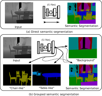
Figure 1: Conventional semantic segmentation vs Our group-wise semantic segmentation. The proposed grouped semantic segmentation method estimates labels of the visible objects from each group and also the visibility of the individual groups which could be further merged together to get the semantic labels. Thus, our method generates more information that an agent could utilize for indoor / outdoor navigation. (See the results in Fig. 5)

To our knowledge there is relatively little literature aiming to predict properties of hidden object parts such as extending the semantic category to unseen surfaces. There is a large body of literature on standard semantic image segmentation, and we refer to [1] for a relatively recent survey. If we go back to classical object detection methods estimating bounding boxes (such as [2]), one can argue that such multi-class object detection approaches already provide a coarse idea on the total extent of a partially occluded object. This observation was e.g. used in [3] to reason about layered and depth-ordered image segmentation. A more refined approach to bounding-box based object detection is semantic instance segmentation (e.g. [4, 5, 6, 7]), which provide finer-grained cues to reason about occluded object parts. We bypass explicit object detection or instance segmentation by directly predicting labels for all categories present (visible or occluded) at each pixel.

This work is closely related to amodal segmentation works [12, 13, 14]. Generally, amodal perception refers to the intrinsic ability of humans to perceive objects as complete even if they are only partially visible. We refer to [15] for an introduction and discussion related to (3D) computer vision. Our work differs from earlier works [12, 13] as our approach predicts amodal segmentation masks for the entire input image (instead of predicting masks only for individual foreground objects). We also target amodal segmentation for rich environments such as indoor scenes and urban driving datasets. We also leverage synthetic training data generation instead of imprecise human annotations.

More recently, there are several attempts to use deep learning to either complete shapes in 3D from single depth or RGB images (e.g. [8, 9]) or to estimate a full semantic voxel space from an RGB-D image [10]. The utilization of a volumetric data structure enables a very rich output representation, but severely limits the amount of detail that can be estimated. The output voxel space used in [10] has a resolution of about $50^{3}$ voxels. The use of 3D voxel space (for input and output) and 3D convolutions also limits the processing efficiency. The low-resolution output space can be addressed e.g. by multi-resolution frameworks (such as [11]), but we believe that image-space methods are more suitable (and possibly more biologically plausible) than object-space approaches.

In summary, our contributions in this work are as follows:

• We propose a new method for semantic segmentation going beyond assigning categories for visible surfaces, but also estimating semantic segmentation for occluded objects and object parts.

• Using the SUNCG dataset we create a new dataset to train deep networks for the above-mentioned segmentation task.

• We show experimentally that a CNN architecture for regular semantic segmentation is also able to predict occluded surfaces without the necessity to enrich the network’s capacity.

The last item suggests that predicting the semantic labels of occluded parts is as a classification problem not significantly more difficult than regular semantic segmentation, and that there are likely synergies between estimating object categories for directly visible and occluded parts. Hence, one of the main practical issues is the generation of real-world training data, which we evade by leveraging synthetic scenes. A schematic comparison of our method against the traditional semantic segmentation is illustrated in Fig. 1.

This paper is organized as follows: section II formalizes the overall problem and present our solution, and section III describes the generation of the dataset and the obtained qualitative and quantitative evaluation. Finally, section IV concludes this work and outlines future work.

II Learning to segment visible and hidden surfaces

In this section we describe our proposed formulation in more detail. We start with illustrating the semantic grouping strategy, which is followed by specifying the utilized loss function and CNN architecture.

II-A Semantic grouping

The proposed grouping strategy is intuitively based on the criterion that objects in a particular group do not necessarily occlude another objects from the same group. On the other hand objects from separate groups can occlude each other. Examples of such grouping can be found in section III-A. For example the “Chair-like” group in Table I contains similar looking objects ’chair’, ’table$\_$and$\_$chair’, ’trash$\_$can’, and ’toilet’ from living room, dining room, kitchen and toilet respectively. Thus each of those objects usually do not occur simultaneously in a particular image. Note that multiple occurrences of a particular object may occlude each other and such self-occlusions are not incorporated. At this point we rather focus on inter-group object category occlusions.

Let there be $N$ different objects categories $[\mathcal{O}_{1},\;\mathcal{O}_{2},\;\ldots,\mathcal{O}_{N}]$ in the scene. The task of semantic segmentation is to classify the pixels of an image to one of those $N$ object categories. A pixel $p$ is marked as a particular category $\mathcal{O}_{j}$ if the posterior probability of the object category $\mathcal{O}_{j}$ is maximum at the pixel $p$. A straight-forward cross-entropy loss is generally utilized in the literature for the said task. As discussed before, the current loss is limited to classifying directly visible objects, i.e., if an object category is visible in a particular pixel, we enforce posterior probability to be $1$ at that pixel else $0$ through cross-entropy loss. In this work, we push it further and allow multiple semantic labels to be active for each pixel. The output of the trained classifier also indicates which of these active labels is corresponding to the directly visible category, which therefore yields the standard semantic segmentation output. However, we do not directly infer a full depth ordering of objects and their semantic categories (which we leave as future work). Rather, we classify each pixel into one of $M$ different groups, where the grouping is based on usual visibility relations. Each group contains a number of finer-grained object categories in addition to a “void” category indicating absence of this group category. Therefore, a pixel will be ideally assigned to a visible and also all occluded object categories.

We group $N$ objects into $M+1$ different groups $[\mathcal{G}_{0},\;\mathcal{G}_{1},\;\mathcal{G}_{2},\;\ldots,\mathcal{G}_{M}]$ where the group $\mathcal{G}_{i}$ contains $g_{i}=|\mathcal{G}_{i}|$ object categories, i.e., $\sum_{i=0}^{M}g_{i}=N$. Note that $g_{i}$’s are not necessarily equal, and different groups can have different number of object categories. Our assumption is that an objects category $\mathcal{O}_{i_{k}}\in\mathcal{G}_{k}$ do not occlude another object category $\mathcal{O}_{j_{k}}\in\mathcal{G}_{k}$. The group $\mathcal{G}_{0}$ is considered as the back-ground. We extend $\mathcal{G}_{i}$ by a “void” category $\varnothing$, yielding $\mathcal{G}_{i}:=\mathcal{G}_{i}\cup\{\varnothing\}$ for $i=1,\dotsc,M$. The “void” category (with corresponding index 0) indicates absence of the group category at that pixel and is not used in the background group $\mathcal{G}_{0}$. An example of such grouping is displayed in Fig. 2.

II-B Semantic segmentation output and loss

II-B1 Conventional Method

The baseline methods for semantic segmentation compute pixel-wise soft-max over the final feature map combined with the cross-entropy loss function. Note that for an image of size $h\times w$, the network $f(.)$ produces feature map of size $h\times w\times N$. The soft-max computes the posterior probability of each pixel belonging to a particular class, which is computed as $p_{c}(x)=\exp(\alpha_{c}(x))/\left(\sum_{c^{\prime}=1}^{N}\exp(\alpha_{i^{\prime}}(x))\right)$, where $\alpha_{c}(x)=f_{c}(x;I)$ is the final layer activation in $i$th feature channel (corresponding to $c$th class) at the pixel position $x$ for input image $I$. In other words $(p_{1}(x),\dots p_{N}(x))$ is an element from the $N$-dimensional probability simplex $\Delta^{N}$. Note that number of activations $N$ is the same as the number of object categories. The energy function is defined by the multi-label cross-entropy loss function for semantic segmentation as follows

$$\mathcal{L}_{CE}=\sum_{x\in\Omega}\log p_{c^{*}(x)}(x),$$ (1)

where $c^{*}(x)$ is the provided ground truth semantic label at pixel $x$ and $\Omega$ is the image domain.

II-B2 Proposed Method

(a) Visible Sem-Seg	(b) Group $\mathcal{G}_{0}$:“Background”	(c) Group $\mathcal{G}_{1}$:“rhombus-like”	(d) Group $\mathcal{G}_{2}$:“circle-like”

Figure 2: An example of the group-wise visibility of four different groups is displayed. A particular color code represent an object category present in a group. The “void” category $\varnothing$ is not marked with any color. $\Omega_{c}^{vis}$ is marked with a darker color whereas $\Omega_{c}^{occ}$ is marked with a lighter color. Note that $\Omega_{c}^{pres}=\Omega_{c}^{vis}\cup\Omega_{c}^{occ}$.

In our proposed formulation the classification output more structured than above (where the output is an element from the $N$-dimensional probability simplex). In our setting the prediction is an element from a product space over probability simplices,

$${\cal Y}:=\Delta^{(M+1)}\times\prod\nolimits_{i=0}^{M}\Delta^{g_{i}+1},$$ (2)

where $(M+1)$ is the number of object groups, and $g_{i}=|\mathcal{G}_{i}|$ is the number of object categories in group $i$. We write an element from $\cal Y$ as $(p,q^{0},q^{1},\dotsc,q^{M})$, where $p\in\Delta^{(M+1)}$ and $q^{i}\in\Delta^{g_{i}+1}$ for all $i=0,1,\dotsc,M$. We use an argument $x$ to indicate the prediction at pixel position $x$. A perfect prediction would have $p(x)$ and all $q_{i}(x)$ at the corner of the respective probability simplex with $p_{i}(x)=1$ if the $i$-th subgroup is visible, and $q^{i}_{j}(x)=1$ for $j\geq 1$ if the $j$-th object category in $\mathcal{G}_{i}$ is present (directly visible or occluded). If none of the categories in $\mathcal{G}_{i}$ is present, then we read $q^{i}_{0}(x)=1$, i.e. index ‘$0$’ of each group corresponds to the “void” category.

One extreme case is if $|\mathcal{G}_{i}|=1$, i.e. each group contains exactly one object category. Then our representation amounts to independently predicting object classes that are present ($q^{i}_{1}(x)=1$) and which of these object categories is directly visible in the image at pixel $x$ (via $p_{i}(x)$). We utilize larger groups for efficiency.

Further note that there are intrinsic constraints on element from $\cal Y$ to be physically plausible. If a group $i$ is estimated to be visible at pixel $x$ ($p_{i}(x)=1$), then $q^{i}_{0}(x)$ has to be 0, as some category from group $i$ is estimated to be observed directly. One can encode such constraints as inequality constraints $p_{i}(x)\leq 1-q^{i}_{0}(x)$ (or $p_{i}(x)\leq\sum_{j=1}^{g_{i}}q^{i}_{j}(x)$ as $\sum_{j=0}^{g_{i}}q^{i}_{j}(x)=1$). For simplicity we do not enforce this constraints at test time and therefore rely on physically plausible training data (always, $p_{i}(x)\leq 1-q^{i}_{0}(x)$) in order for the network to predict only plausible outputs. Refer to sec. III-C for further analysis.

Note that standard semantic segmentation can also be inferred from our group-wise segmentation, e.g. by assigning the semantic label corresponding to $\max_{i}p_{i}(x)\max_{j=1,\dotsc,g_{i}}q^{i}_{j}(x)$. The details of the procedure is described in sec. III-C. In the experiment section, we show that we observe similar performance for the task of semantic segmentation by a similar network trained with the conventional method. Thus with a network architecture almost identical to one for standard semantic segmentation, our proposed output representation additionally estimates semantic labels of occluded back-ground and inter-group occluded object categories with nearly the same number of parameters (only the output layer differs).

II-B3 Modified loss function

For a given image and ground truth semantic label $c^{*}(x)$ at pixel $x$, let $i^{*}(x)$ be the semantic group such that $c^{*}(x)\in\mathcal{G}_{i^{*}(x)}$ and let $j^{*}(x)\neq 0$ be the (non-“void”) element in $\mathcal{G}_{i}$ corresponding to category $c^{*}(x)$. Let $\mathcal{C}(i,j)$ be the reverse mapping yielding the category corresponding to group $i$ and index $j$ (for $j\geq 1$). Let $\Omega_{c}^{vis}\subseteq\Omega$ be the image regions labeled with category $c$, i.e. pixels where category $c$ is directly visible. Further we are given $N$ sets $\Omega^{pres}_{c}\subseteq\Omega$ that indicate whether category $c$ is present (directly visible or occluded) at a pixel. Now $\Omega_{c}^{occ}=\Omega_{c}^{pres}\setminus\Omega_{c}^{vis}$ is the set of pixels where category $c$ is present but not directly visible. Finally, $\Omega_{i}^{\varnothing}:=\Omega\setminus\left(\bigcup_{j\in\mathcal{G}_{i}}\Omega^{pres}_{c(i,j)}\right)$ is the set of pixels where no category in group $i$ is present. With these notations in place we can state the total loss function as

$$\mathcal{L} =\mathcal{L}_{g}+\sum\nolimits_{i=0}^{M}\mathcal{L}_{i}$$ (3)

with

$$\mathcal{L}_{g} =\sum_{x\in\Omega}\log p_{i^{*}(x)}(x)$$ (4)

$$\mathcal{L}_{i} =\sum_{j\in\mathcal{G}_{i}}\left(\sum_{x\in\Omega^{vis}_{c(i,j)}}\log q^{i}_{j}(x)+\lambda\sum_{x\in\Omega^{occ}_{c(i,j)}}\log q^{i}_{j}(x)\right)$$ (5)

$$~{}~{}~{}~{}~{}~{}~{}~{}~{}~{}~{}~{}~{}~{}~{}~{}~{}~{}~{}~{}~{}~{}~{}~{}~{}~{}~{}+\lambda\sum_{x\in\Omega_{i}^{\varnothing}}\log q^{i}_{0}(x).$$

$\mathcal{L}_{g}$ is a standard cross-entropy loss such that the correct visible group is predicted. For each group $i$ we have a cross-entropy loss aiming to predict the correct visible index $j$ in group $i$ (with full weight) and occluded indices (with weighting $\lambda$). Throughout all of our experiments the weight proportion $\lambda$ is chosen as $0.1$.

II-C Architecture

We utilize a standard semantic segmentation architecture (U-Net [16]) with a deep CNN. It consists of an encoder and a decoder which are sequences of convolutional layers followed by instance normalization [17] layers and ReLus except for the last layer where a sigmoid activation function is utilized followed by group-wise soft-max. Skip connections from encoder to decoder are also incorporated in the architecture.

In the proposed representation, the prediction is an element from a product space over probability simplices in the form of $(p,q^{0},q^{1},\dotsc,q^{M})$, where $p\in\Delta^{(M+1)}$ and $q^{i}\in\Delta^{g_{i}+1}$ for all $i=0,1,\dotsc,M$. Therefore number of activations at the group-wise soft-max layer $(M+1)+\sum_{i=0}^{M}(g_{i}+1)=2(M+1)+\sum_{i=0}^{M}g_{i}=2(M+1)+N$. Thus we require only extra $2(M+1)$ activations compared to the conventional semantic segmentation with cross-entropy loss. Further, we use only a small number of groups (for example, our dataset consists of five groups and consequently requires $12$ more activations), thus proposed method comprises approximately similar number of parameters [see Fig. 3].

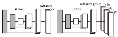
(a) Direct Sem-Seg

(b) Grouped Sem-Seg

Figure 3: Conventional semantic segmentation vs Our group-wise semantic segmentation: (a) in the conventional semantic segmentation there are $N$ number of activations and (b) in the proposed method we have $2(M+1)+N$ activation layers. For details see the text.

III Evaluation

The proposed segmentation method is evaluated with a standard semantic segmentation architecture (described in sec. II-C) on a newly developed dataset, augmented from SUNCG [10] (details are in the following section). The loss $\mathcal{L}$ (eqn. (3)) is minimized using ADAM with a mini-batch of size $25$. The weight decay is set to $10^{-5}$. The network is trained for $100$ epochs with an initial learning rate $0.001$ which is gradually decreased by a factor of $10$ after every $10$ epochs. A copy of same set of parameters is utilized for the baseline method. The architecture is implemented in Python and trained with Tensorflow on a desktop equipped with a NVIDIA Titan X GPU and an Intel CPU of $3.10GHz$.

TABLE I: The partition of objects into different Groups of SUNCG [10]

Groups $\mathcal{G}_{i}$	Objects $\mathcal{O}_{j}$ in the group
Group $\mathcal{G}_{0}$: Background	’ceiling’, ’floor’, ’wall’, ’window’, ’door’
Group $\mathcal{G}_{1}$: Chair-like	’chair’, ’table$\_$and$\_$chair’, ’trash$\_$can’, ’toilet’
Group $\mathcal{G}_{2}$: Table-like	’table’, ’side$\_$table’, ’bookshelf’, ’desk’
Group $\mathcal{G}_{3}$: Big Objects	’bed’, ’kitchen$\_$cabinet’, ’bathtub’, ’mirror’,
	’closets$\_$cabinets’, ’dont$\_$care’, ’sofa’
Group $\mathcal{G}_{4}$: Small Objects	’lamp’, ’computer’, ’music’, ’gym’, ’pillow’,
	’household$\_$appliance’, ’kitchen$\_$appliance’,
	’pets’, ’car’, ’plants’, ’pool’, ’recreation’,
	’night$\_$stand’, ’shower’, ’tvs’, ’sink’

In addition, as discussed before, a “void” category is inserted in each group

indicating absence of the object categories in the group while rendering.

III-A Datasets

We could not find any suitable dataset for the current task. As described above, the amodal semantic segmentation dataset [13] does not serve our purpose. Note that we require group-wise semantic labels for the evaluation, thus the following datasets are leveraged in this work:

III-A1 SUNCG [10]

• It is a large-scale dataset containing $6,220$ synthetic 3D models of indoor scenes. Further, it provides a toolbox to select camera poses at informative locations of the 3D scene. The toolbox generates $22,742$ distinct camera poses which are further augmented $20$ times with random traversal at the nearby poses. The random traversals are considered as Gaussians with standard deviations $1$m and $15^{\circ}$ for translations and rotation respectively. The camera poses are further refined to get $159,837$ distinct camera poses. We incorporate following heuristics for the refinement, i.e., remove non-informative camera poses if

  • the scene does not contain any other objects excluding background object categories inside the viewing frustum of the camera pose,

  • there is substantial portion ($40\%$) of an object placed very close to the camera (within $1$m of the camera center) and inside the viewing frustum,

  • more than $40\%$ of the ground-truth pixel labels are assigned to ‘dont$\_$care’ object category, etc.

• For a given scene (a synthetic 3D model) and a camera pose, the toolbox also provides a rendering engine that generates depth images and semantic labels of $36$ object categories. The depth image and semantic label image pair can be used as a ground-truth training image pair to train a conventional direct semantic segmentation method.

• To generate ground-truths for the proposed group-wise semantic segmentation, the object categories are further grouped intuitively into $5$ different groups as described in Table I and are rendered individually. Note that no optimal strategy for grouping is utilized in this work. The ground-truth occlusions among the different groups are generated as follows—remove all the objects in the scene and place only the objects present in each group one at a time. The rendering engine is then applied to each group to generate the semantic labels of the objects present in the group. Examples of the ground-truth dataset can be found in Fig. 4.

• A similar strategy is applied to $155$ synthetic test 3D models to generate $873$ ground-truth test images. Note that we used the same partition of the training and test 3D models provided by the dataset.

	(a) Depth	(b) Sem-Seg	(c) $\mathcal{G}_{0}$	(d) $\mathcal{G}_{1}$	(e) $\mathcal{G}_{2}$	(f) $\mathcal{G}_{3}$	(g) $\mathcal{G}_{4}$

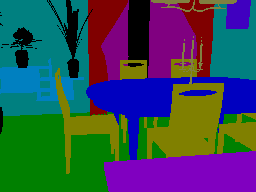
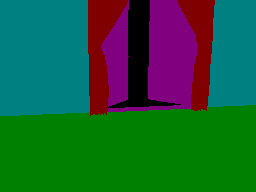
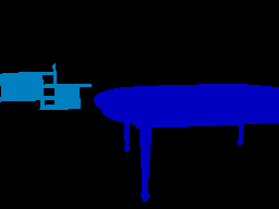
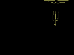
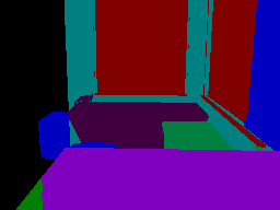
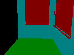
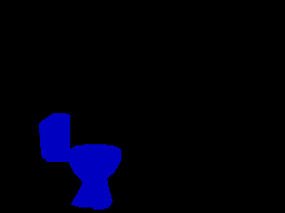
Figure 4: Examples of images of our synthesized dataset tailored from SUNCG Datasets [10]. Note that given a single depth image (a), the task is to estimate the semantic labels of the different objects present in the scene, along with predict individual groups $[\mathcal{G}_{0},\;\mathcal{G}_{1},\;\mathcal{G}_{2},\;\ldots,\mathcal{G}_{M}]$ of different objects. See sec. III-A for the details. The “void” category $\varnothing$ is marked by black pixels.

III-A2 Cityscape [18]

• A real large-scale dataset for semantic segmentation on real driving scenarios. The original dataset does not include amodal perception (i.e., separate visible / occluded labels for each pixel).

• To evaluate the proposed method in this dataset, the objects are divided into $3$ different groups as described in Table II. Similar to SUNCG dataset, we follow an intuitive strategy to group the objects. However in this scenario, it is hard to generate a real dataset of semantic labels of the occluded objects. A similar strategy of [12] is adapted to generate the training dataset. We randomly duplicate mobile objects on relevant locations—for example, ‘car’, ‘truck’, ‘bus’ on the ‘road’ and ‘person’, ‘rider’ on the ‘sidewalk’—and corresponding visible (newly placed object label) and occluded (original semantic label) locations are utilized for training. During training the network hallucinates the occluded labels which is matched against the ground-truth occluded labels (ignored if unavailable) and penalizes any miss-predictions. Note that during testing our method only takes a real rgb image and generate semantic visible layers of each group (described in Table II).

• The detailed results are furnished in sec. III-E.

TABLE II: The partition of object categories of Cityscape dataset [18]

Groups	Objects in the group
Group $\mathcal{G}_{0}$: Background	’road’, ’sidewalk’, ’wall’, ’building’, ’sky’,
	’terrain’, ’fence’, ’vegetation’
Group $\mathcal{G}_{1}$: Traffic Objects	’pole’, ’traffic light’, ’traffic sign’
Group $\mathcal{G}_{2}$: Mobile Objects	’person’, ’rider’, ’car’, ’truck’, ’bus’,
	’motocycle’, ’train’, ’bicycle’

III-B Baseline Methods

The evaluation is conducted amongst following baselines:

• The conventional semantic segmentation network (U-net [16] architecture) with cross-entropy loss named as Direct Semantic Segmentation (DSS). The final semantic segmentation result is abbreviated as Sem-Seg.

• A similar architecture is utilized for the proposed group-wise segmentation–instead of direct pixel-wise classification a group-wise classification is introduced as described in sec. II-A. We abbreviate the proposed method as Grouped Semantic Segmentation (GSS).

Note that in this work, we emphasize on group-wise (e.g., “Chair-like”) segmentation for the task of semantic labeling of the occluded objects compared to conventional semantic segmentation methods. Therefore the proposed method is not evaluated against different types of semantic segmentation architectures. Further, our group-wise model can be adapted to any of the existing sophisticated architectures.

	(a) Input	(b) $\mathcal{G}_{0}$	(c) $\mathcal{G}_{1}$	(d) $\mathcal{G}_{2}$	(e) $\mathcal{G}_{3}$	(f) $\mathcal{G}_{4}$	(g) Sem-Seg

Figure 5: Qualitative results on SUNCG Datasets [10]. Note that the floor parts are hallucinated almost perfectly. See sec. III-D for more details.

III-C Quantitative Evaluation

Many evaluation criteria have been proposed in the literature to assess the quality of the semantic segmentation methods. In this work, we adapt existing matrices and tailor in the following way to tackle occlusions

• Visible Pixel Accuracy ($\text{PA}^{vis}$): It is the ratio between properly classified (visible) pixels and the total number of them. Let $\Omega_{c}^{vis}$ and $\widehat{\Omega}_{c}^{vis}$ be the set of all pixels actually visible and predicted visible with class-label $c$ respectively.

  $$\text{PA}^{vis}=\frac{\sum_{c=1}^{N}|\Omega_{c}^{vis}\cap\widehat{\Omega}_{c}^{vis}|}{|\Omega|}$$ (6)

• Visible Mean Intersection over Union ($\text{MIoU}^{vis}$): It is the conventional metric for segmentation purposes and redefined similarly. It is the ratio between the intersection and the union of two sets—the ground truth visible and our predicted visible. It can be written as

  $$\text{MIoU}^{vis}=\frac{1}{N}\sum_{c=1}^{N}\frac{|\Omega_{c}^{vis}\cap\widehat{\Omega}_{c}^{vis}|}{|\Omega_{c}^{vis}\cup\widehat{\Omega}_{c}^{vis}|}$$ (7)

  The IoU is computed on a per class basis and then averaged. Note that $\text{PA}^{vis}$ and $\text{MIoU}^{vis}$ are the same as conventional pixel accuracy and mean intersection over union used in the semantic segmentation literature.

• Present Pixel Accuracy ($\text{PA}^{pres}$): It is defined in a similar way to $\text{PA}^{vis}$ where in this case the numerator is calculated over the pixels where the object is present (visible / occluded). Let $\Omega_{c}^{pres}$ and $\widehat{\Omega}_{c}^{pres}$ be the set of all pixels actually present (visible / occluded) and predicted present with class-label $c$ respectively.

  $$\text{PA}^{pres}=\frac{\sum_{c=1}^{N}|\Omega_{c}^{pres}\cap\widehat{\Omega}_{c}^{pres}|}{|\Omega|}$$ (8)

• Present Mean Intersection over Union ($\text{MIoU}^{pres}$): It is defined in the similar fashion

  $$\text{MIoU}^{pres}=\frac{1}{N}\sum_{c=1}^{N}\frac{|\Omega_{c}^{pres}\cap\widehat{\Omega}_{c}^{pres}|}{|\Omega_{c}^{pres}\cup\widehat{\Omega}_{c}^{pres}|}$$ (9)

Note that $(\Omega_{c}^{vis},\;\Omega_{c}^{pres})$ are readily available from the ground truth dataset and $(\widehat{\Omega}_{c}^{vis},\;\widehat{\Omega}_{c}^{pres})$ are estimated by baseline methods. The conventional DSS estimates $\widehat{\Omega}_{c}^{vis}$ (set of the pixels predicted with category $c$), however, $\widehat{\Omega}_{c}^{pres}$ is not readily available. It can be obtained by computing indices of the maximum posterior probability of the group (+background) that object category $c$ belongs to i.e.,

$$\widehat{\Omega}_{c}^{pres}=\{x|c=\arg\max_{j\in I_{i}}p_{j}(x)\}$$ (10)

where category $c$ belongs to the group $\mathcal{G}_{i}$, $p_{j}(x)$ is the posterior probability of the $j$th class category at pixel $x$, and $I_{i}$ is the set of indices corresponds to object categories in the set $\mathcal{G}_{0}\cup\mathcal{G}_{i}$. The indices of $\mathcal{G}_{0}$ are squashed to the “void” category $\varnothing$. If $c$ belongs to the background class $\mathcal{G}_{0}$, the index set $I_{i}$ is chosen from the indices of $\mathcal{G}_{0}$ only and no squashing is required in this case.

Similarly, the GSS directly estimates $\widehat{\Omega}_{c}^{pres}$ whereas $\widehat{\Omega}_{c}^{vis}$ is again not readily available and computed in the following manner:

$$\widehat{\Omega}_{c}^{vis} =\{x|c=\mathcal{C}(\hat{i},\;\hat{j})\text{~{}where~{}}\hat{i}=\max_{i}p_{i}(x)$$ (11)

$$~{}~{}~{}~{}~{}~{}~{}~{}~{}~{}~{}~{}~{}~{}~{}~{}~{}~{}~{}~{}~{}~{}~{}~{}\text{~{}and~{}}\hat{j}=\max_{j=1,\dotsc,g_{i}}q^{i}_{j}(x)\}$$

$$=\widehat{\Omega}_{\mathcal{G}_{i}}^{vis}\cap\widehat{\Omega}_{c}^{pres}$$ (12)

where $\mathcal{C}(i,j)$ be the reverse mapping yielding the category corresponding to group $i$ and index $j$ and $\widehat{\Omega}_{\mathcal{G}_{i}}^{vis}$ are the visible pixels of the group that the category $c$ belongs to.

The quantitative results are presented in Table III. The conventional DSS is trained with visible semantic labels [Fig. 4(b)] and the proposed GSS method is trained with visible + occluded [Fig. 4(b)-(c)] semantic labels. We observe GSS performs analogously with DSS for the task of conventional semantic segmentation (i.e., visible pixels). However, for the regions where the objects are present (visible / occluded) proposed GSS performs much better. To make it clear that the better performance of GSS is not driven by the inclusion of the “void” category, we present results with / without the “void” class separately. Therefore given a fixed network capacity and with the availability of data, the proposed GSS exceeds the conventional method for the task of semantic labeling of the occluded objects.

TABLE III: Quantitative Evaluation on the augmented SUNCG [10]

	Visible		Present Regions		Present Regions
Methods	Regions		with “void” $\varnothing$		without “void” $\varnothing$
	$\text{PA}^{vis}$	$\text{MIoU}^{vis}$	$\text{PA}^{pres}$	$\text{MIoU}^{pres}$	$\text{PA}^{pres}$	$\text{MIoU}^{pres}$
DSS	$\bf{0.850}$	$\bf{0.575}$	$0.715$	$0.268$	$0.755$	$0.594$
GSS	$0.833$	$0.551$	$\bf{0.900}$	$\bf{0.470}$	$\bf{0.861}$	$\bf{0.645}$

III-D Qualitative Evaluation

The qualitative comparison of the selected baseline methods on test dataset is displayed in Fig. 5. The methods take the depth image [Fig. 5(a)] as an input and predicts the semantic segmentation [Fig. 5(b)] as an output. Further, the proposed GSS is also computed as described in the above and displayed in Fig. 5(c)-(g). We observe that conventional Sem-Seg could hallucinate the occluded objects in some cases, however, the network finds difficulty estimating “void” class which is essential to model the correct occlusion. For example, in the first row of Fig. 5, the object class “Bed” covers / occlude the entire floor and the conventional DSS could able to hallucinate the occluded floor, however, it further hallucinates other objects categories present in the other groups.

The proposed GSS performs consistently well on task of semantic segmentation of the visible and the occluded objects. Unlike the DSS, we do not observe any difficulty estimating the “void” category. The estimated background also looks much cleaner. Note that the examples are not cherry-picked and are quite random from the test data.

III-E Qualitative Evaluation on Cityscape [18]

The training datasets for cityscape are augmented by placing the mobile objects randomly around the neighborhood (see sec. III-A for details). During testing, the network only observes a real rgb image (in contrast to SUNCG [10] that observes a single depth image) and produces the semantic labels for each group. An example result and its cropped version is shown in Fig. 6.

	(a) Input	(b) $\mathcal{G}_{0}$: Background	(c) $\mathcal{G}_{1}$: Traffic Objects
		(d) $\mathcal{G}_{2}$: Mobile Objects	(e) Sem-Seg
	Cropped–(a) Input	Cropped–(b) $\mathcal{G}_{0}$: Background	Cropped–(c) $\mathcal{G}_{1}$: Traffic Objects
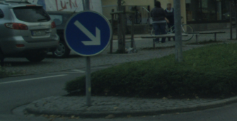
		Cropped–(d) $\mathcal{G}_{2}$: Mobile Objects	Cropped–(e) Sem-Seg

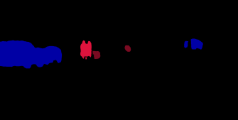
Figure 6: Qualitative results of an image from Cityscape datasets and its cropped version of a region of interest. Notice that the car, hidden behind the traffic signal (marked by the yellow box in (a) and then later zoomed in Cropped-(a)), is fully recovered in the ‘$\mathcal{G}_{2}$: mobile objects’ layer (d). However, the traffic signal wrongly cut the pavements into parts (Cropped-(d)) in the ‘$\mathcal{G}_{0}$: Background’ layer.

IV Conclusion and future work

In this work we aim to push the boundaries of assigning semantic categories only to visible objects. A group-wise semantic segmentation strategy is proposed, which is capable of predicting semantic labels of the visible objects along with semantic labels of the occluded objects and object parts without any necessity to enrich the network capacity. We develop a synthetic dataset to evaluate our GSS. A standard network architecture trained with proposed grouped semantic loss performs much better than conventional cross-entropy loss for the task of predicting semantic labels of the occluded pixels. The dataset along with the scripts of the current work will be released to facilitate research towards estimating semantic labels of the occluded objects.

Currently the training set, leveraged in this work, is purely synthetic, but it allows strongly supervised training. This limits the applicability of the proposed method to environments having a suitable synthetic models available. Hence, future work will address how to incorporate weaker supervision in this problem formulation in case of a real dataset and also incorporate uncertainty estimation of the occluded regions.

References

- [1] Garcia-Garcia, A., Orts-Escolano, S., Oprea, S., Villena-Martinez, V., Garcia-Rodriguez, J.: A review on deep learning techniques applied to semantic segmentation. arXiv:1704.06857 (2017)
- [2] Redmon, J., Divvala, S., Girshick, R., Farhadi, A.: You only look once: Unified, real-time object detection. In: ICCV. (2016) 779–788
- [3] Yang, Y., Hallman, S., Ramanan, D., Fowlkes, C.: Layered object detection for multi-class segmentation. In: CVPR. (2010) 3113–3120
- [4] Hariharan, B., Arbeláez, P., Girshick, R., Malik, J.: Simultaneous detection and segmentation. In: ECCV. (2014) 297–312
- [5] Dai, J., He, K., Sun, J.: Instance-aware semantic segmentation via multi-task network cascades. In: ICCV. (2016) 3150–3158
- [6] He, K., Gkioxari, G., Dollár, P., Girshick, R.: Mask R-CNN. In: ICCV. (2017) 2980–2988
- [7] Kirillov, A., He, K., Girshick, R., Rother, C., Dollár, P.: Panoptic segmentation. arXiv:1801.00868 (2018)
- [8] Wu, Z., Song, S., Khosla, A., Yu, F., Zhang, L., Tang, X., Xiao, J.: 3D shapenets: A deep representation for volumetric shapes. In: CVPR. (2015) 1912–1920
- [9] Sharma, A., Grau, O., Fritz, M.: VConv-DAE: Deep volumetric shape learning without object labels. In: ECCV. (2016) 236–250
- [10] Song, S., Yu, F., Zeng, A., Chang, A.X., Savva, M., Funkhouser, T.: Semantic scene completion from a single depth image. In: CVPR. (2017) 190–198
- [11] Dai, A., Ritchie, D., Bokeloh, M., Reed, S., Sturm, J., Nießner, M.: Scancomplete: Large-scale scene completion and semantic segmentation for 3d scans. In: CVPR. Volume 1. (2018) 2
- [12] Li, K., Malik, J.: Amodal instance segmentation. In: ECCV, Springer (2016) 677–693
- [13] Zhu, Y., Tian, Y., Metaxas, D., Dollár, P.: Semantic amodal segmentation. In: CVPR. (2017) 1464–1472
- [14] Ehsani, K., Mottaghi, R., Farhadi, A.: Segan: Segmenting and generating the invisible. In: CVPR. (2018) 6144–6153
- [15] Breckon, T.P., Fisher, R.B.: Amodal volume completion: 3d visual completion. CVIU 99 (2005) 499–526
- [16] Ronneberger, O., Fischer, P., Brox, T.: U-net: Convolutional networks for biomedical image segmentation. In: International Conference on Medical image computing and computer-assisted intervention, Springer (2015) 234–241
- [17] Ulyanov, D., Vedaldi, A., Lempitsky, V.: Instance normalization: The missing ingredient for fast stylization. arXiv:1607.08022 (2016)
- [18] Cordts, M., Omran, M., Ramos, S., Rehfeld, T., Enzweiler, M., Benenson, R., Franke, U., Roth, S., Schiele, B.: The cityscapes dataset for semantic urban scene understanding. In: CVPR. (2016) 3213–3223