Devolatilization of Subducting Slabs, Part I:
Thermodynamic Parameterization and Open System Effects

Abstract

The amount of H₂O and CO₂ that is carried into deep mantle by subduction beyond subarc depths is of fundamental importance to the deep volatile cycle but remains debated. Given the large uncertainties surrounding the spatio-temporal pattern of fluid flow and the equilibrium state within subducting slabs, a model of H₂O and CO₂ transport in slabs should be balanced between model simplicity and capability. We construct such a model in a two-part contribution. In this Part I of our contribution, thermodynamic parameterization is performed for the devolatilization of representative subducting materials—sediments, basalts, gabbros, peridotites. The parameterization avoids reproducing the details of specific devolatilization reactions, but instead captures the overall behaviors of coupled (de)hydration and (de)carbonation. Two general, leading-order features of devolatilization are captured: (1) the released volatiles are H₂O-rich near the onset of devolatilization; (2) increase of the ratio of bulk CO₂ over H₂O inhibits overall devolatilization and thus lessens decarbonation. These two features play an important role in simulation of volatile fractionation and infiltration in thermodynamically open systems. When constructing the reactive fluid flow model of slab H₂O and CO₂ transport in the companion paper Part II, this parameterization can be incorporated to efficiently account for the open-system effects of H₂O and CO₂ transport.

I Introduction

Subduction zones are sites where two tectonic plates converge and one descends beneath the other. As subduction proceeds, the warm ambient mantle heats the downgoing plate, which sinks to increasing depth and pressure. The thermal and mechanical changes drive chemical reactions in the slabs, among which devolatilization reactions are of particular importance because they induce flux melting, trigger seismic activity, and mobilize diagnostic chemical species observed in arc lava chemistry [see 1, for a review]. When it comes to global volatile cycling, especially H₂O and CO₂, controversy persists regarding where and how much H₂O & CO₂ release occurs in subducting slabs [2, 3, 4, 5]. For example, Dasgupta et al. [3] and Gorman et al. [4] argue that subduction brings more CO₂ into the deep mantle than the amount emitted from arc volcanoes, based respectively on experiments and thermodynamic modelling. However, after compiling CO₂ flux data from field studies and extrapolating modelling results, Kelemen and Manning [5] contends that almost all the subducted CO₂ is returned to the overriding lithosphere or surface during subduction. Studies focusing only on H₂O transport in subduction zones also yield disparate conclusions with regard to the efficiency of H₂O recycling into the deeper mantle: Hacker [6] and van Keken et al. [7] suggest that 35–54% of subducted H₂O is recycled to mantle depths beyond $\sim$150 km, whereas Wada et al. [8] argues that only half of this amount is recycled if the subducting slab is heterogeneously hydrated as opposed to uniformly hydrated.

Large uncertainties surround the attempt to quantify the H₂O and CO₂ fluxes within and from subducting slabs. On the dynamic side, the style and pathways of volatile migration is poorly constrained. Field evidence shows that fluid flow proceeds through both porous and fractured rocks [see 9, for a review] and numerical models suggest that fluid migration can take place via porosity waves [10], fractures [11], and large-scale faults [12]. Recent geochemical studies indicate that fluid explusion during subduction might be episodic rather than steady [13]. On the thermodynamic side, although it is known that metamorphic devolatilization reactions control the release of slab H₂O and CO₂, it remains unclear whether or not these reactions achieve equilibrium or overstep it [e.g. 14, 15, 16]. Moreover, earlier experimental work [17] shows that the dihedral angle between mineral grains coexisting with released volatiles is highly variable and can prevent the formation of an inter-connected pore network during subduction.

On top of the uncertainties above, from a modelling perspective, a computational obstacle in quantifying the H₂O & CO₂ budget in subducting slabs comes from thermodynamically open-system behavior. Volatiles that are released during devolatilization reactions are buoyant relative to surrounding rocks and tend to migrate [e.g., 11]. As conventional thermodynamic computation for chemical equilibrium assumes closed systems [e.g., 18, 19], the open-system behavior caused by volatile migration makes it challenging to model the slab H₂O & CO₂ budget. To circumvent this challenge, Gorman et al. [4] approximate the effects of mass transfer by adjusting the bulk H₂O & CO₂ content of the modelled rocks according to simple rules inspired by buoyancy-driven flow. The adjustment is premised on pre-defined fluid flow pathways, along which upstream H₂O & CO₂ is added to downstream bulk compositions and re-equilibration is repetitively calculated. Such an approach is advantageous in providing all the thermodynamic information of the modelled system, e.g., mineral mode, composition, density, etc., but suffers from oversimplification in assuming upward fluid migration. In contrast, fluid dynamical calculations [20] show a substantial up-slab fluid flow during subduction. Another way of treating open-system behaviors comes from studies of magma dynamics where percolation of partially molten melts causes mass transport [e.g., 21, 22]. The essence of this approach lies in the simplification of thermodynamics, such that the computational cost of thermodynamic calculation becomes affordable when it is coupled with fluid dynamic simulations. Its advantage is therefore a consistent treatment of the flow and reactions.

However, given the large uncertainties regarding the dynamics and thermodynamics of volatile transport in subducting slabs, it is important to focus on robust, leading-order phenomena in constructing models to evaluate the H₂O & CO₂ budget and fluxes in the slabs. The leading-order factors in our consideration are: the coupling between (de)hydration and (de)carbonation reactions, open-system behaviors caused by volatile transport, and the direction of volatile migration. We handle the coupled dehydration and decarbonation reactions with a thermodynamic parameterization that is amenable to systems open to H₂O & CO₂ transport during subduction. In the companion contribution (Part II), we apply the parameterization to subduction zones to assess the effects of open-system behavior and fluid flow directions on slab H₂O & CO₂ budget and fluxes. The simplified calculations introduced by the parameterization overcome the obstacle of computational cost of this coupling.

In the following, we first present in section II the strategy and formalism adopted to parameterize the subduction-zone devolatilization reactions. The strategy is then applied separately to each representative subducting lithology in section III. In this process, our parameterization ensures two leading-order features: one is that the CO₂ content of the liquid phase increases with temperature and decreases with pressure, as confirmed by previous experiments [e.g., 23]; the other is that preferential H₂O loss from or CO₂ addition to the bulk system raises the onset temperature of devolatilization and thus inhibits it. Through simple examples in section IV, we show that inclusion of these two features enables the parameterization to simulate fractionation and infiltration processes relevant to open-system behaviors [e.g., 4]. An understanding of fractionation and infiltration is crucial for interpreting the results on the H₂O & CO₂ storage and fluxes in the slabs that are presented in the companion manuscript. In section V, the limitations of this thermodynamic parameterization are discussed.

II Strategy and formalism

The goal of our thermodynamic parameterization is, for a specified pressure ($P$), temperature ($T$), and bulk H₂O & CO₂ content of a given lithology, to predict the quantitative equilibrium partitioning of H₂O & CO₂ between solid rock phase and liquid volatile phase. Such a thermodynamic module is therefore applicable to a system that comprises two physical phases of liquid and solid, and multiple chemical components of $\mathrm{Na_{2}O}$, $\mathrm{CaO}$, $\mathrm{SiO_{2}}$, H₂O, CO₂, etc. To make the parameterization tractable, we group all the non-volatile oxides ($\mathrm{Na_{2}O}$, $\mathrm{CaO}$, $\mathrm{SiO_{2}}$, etc.) as a single chemical component. This effective component is designated as rock and resides only in solid phase. Together with the volatile components H₂O and CO₂, the system in consideration is thus a two-phase system of three chemical components.

Directly parameterizing the full three-component system lacks a sound thermodynamic premise to start with (see Appendix A) and can obscure our understanding of the basic behaviors in dehydration and decarbonation of slab lithologies. Therefore, our strategy comprises two steps: (i) parameterize the simpler subsystems rock+H₂O and rock+CO₂ separately; (ii) synthesize the two subsystems into the full system (i.e., rock+H₂O+CO₂) by introducing additional parameters that account for the non-ideal thermodynamic mixing of H₂O and CO₂. This procedure is applied sequentially to lithologies relevant for subducting slabs: sediments, mid-ocean ridge basalts (MORB), gabbros, and mantle peridotites (Table 1).

Table 1: Bulk Compositions for Representative Subducting Lithologies (wt%)

	$\mathrm{SiO_{2}}$	$\mathrm{TiO_{2}}$	$\mathrm{Al_{2}O_{3}}$	$\mathrm{FeO^{T}}$	$\mathrm{MgO}$	$\mathrm{CaO}$	$\mathrm{Na_{2}O}$	$\mathrm{K_{2}O}$	H2O	CO2
MORB	49.33	1.46	15.31	10.33	7.41	10.82	2.53	0.19	2.61	2.88
Gabbro	48.64	0.87	15.48	5.96	8.84	12.02	2.69	0.096	2.58	2.84
Sediment	58.57	0.62	11.91	5.21	2.48	5.95	2.43	2.04	7.29	3.01
Peridotite	44.90	0.20	4.44	8.03	37.17	3.54	0.36	0.029	–	–

The subsystem parameterization employs ideal solution theory [e.g. 24, 25, 22]. In an ideal solution, the dissolution of one chemical component does not affect the chemical potential of other components. Hence the partition coefficient ($K$) of component $i$ between solid and liquid phases can be represented as:

$$K^{i}=\frac{c_{s}^{i}}{c_{l}^{i}}={c_{sat}^{i}(P)}\exp{\left[L_{R}(P)\left(\frac{1}{T}-\frac{1}{T_{d}^{i}(P)}\right)\right]},$$ (1)

where $i$ represents either H₂O or CO₂. Notations of symbols are listed in Table 2 and an exposition of the thermodynamic basis for equation (1) is provided in Appendix A. $T_{d}^{i}(P)$ represents the onset temperature of effectively averaged dehydration or decarbonation in respective subsystems, and $L_{R}(P)$ is the corresponding enthalpy change divided by the gas constant ($R$) for the average reaction, hence termed the “effective” enthalpy change. As a result, this functional form allows a focus on the leading-order behaviors of devolatilization by smoothing out detailed steps of mineral breakdown. Devolatilization is represented by a continuous process where volatiles dissolved in solid rocks exolve into co-existing liquid phases. We describe below how to extract the volatile saturation content ($c^{i}_{sat}$), onset temperature ($T^{i}_{d}$) and effective enthalpy change ($L_{R}$) from results of PerpleX.

Firstly, we use PerpleX [18] to calculate pseudosection diagrams for the subsystems: rock+H₂O or rock+CO₂. For example, non-volatile oxide compositions (Table 1) from representative gabbros [6] are adopted in our PerpleX calculations for the H₂O- and CO₂-saturated subsystems for the gabbroic lithology. Secondly, at each specific pressure, the maximum H₂O (or CO₂) content in gabbros can be extracted from the subsystem output from PerpleX as the corresponding volatile saturation ($c^{i}_{sat}$) content. Over the pressure range of interest (0.5–6 GPa) and with a pressure interval of $\sim$0.007 GPa, extraction at a series of specific pressure values yields a series of saturation values for H₂O (or CO₂), which can be regressed as a function of pressure. Thirdly, to further extract the values for $L_{R}$ and $T^{i}_{d}$ at that specific pressure, equation (1) is transformed to:

$$\ln K^{i}=\ln{{c_{sat}^{i}(P)}}+L_{R}(P)\left(\frac{1}{T}-\frac{1}{T_{d}^{i}(P)}\right).$$ (2)

According to equation (2), when pressure is fixed at a specific value, $L_{R}$ is the slope and $-L_{R}/T^{i}_{d}+\ln{{c_{sat}^{i}}}$ is the intercept if linear regression is performed between $\ln K^{i}$ and $1/T$, where the $K^{i}$ values at different temperatures ($T$) come from the PerpleX results. Fourthly, with the known $c^{i}_{sat}$, $L_{R}$, and the intercept from above, $T_{d}^{i}$ can be obtained at the specific pressure. Similar to step two, the $T^{i}_{d}$ and linearly regressed $L_{R}$ values at various pressures are then fitted with polynomial functions of pressure over the same pressure range of interest.

Table 2: Notations of Symbols in the Equations

Symbol	Meaning	Value and/or Unit
$c^{i}_{s}$	mass fraction of volatile $i$ in solid phase
$c^{i}_{l}$	mass fraction of volatile $i$ in liquid phase
$c^{i}_{blk}$	mass fraction of volatile $i$ in bulk system
$c^{i}_{sat}$	saturated mass fraction of volatile $i$ in solid
$f$	mass fraction of liquid phase in two-phase system
$i$	H2O or CO2
$K^{i}$	ideal partition coefficient of volatile $i$
$\mathcal{K}^{i}$	non-ideal partition coefficient of volatile $i$
$L_{R}$	effective enthalpy change for devolatilization reactions	$\mathrm{K}$
$P$	pressure	GPa
$R$	gas constant	8.314 $\mathrm{J}\ \mathrm{K}^{-1}\ \mathrm{mol}^{-1}$
$T$	temperature	$\mathrm{K}$
$T^{i}_{d}$	onset temperature of devolatilization for volatile $i$ in subsystems	$\mathrm{K}$
$\mathcal{T}^{i}_{d}$	onset temperature of devolatilization for volatile $i$ in full systems	$\mathrm{K}$
$\Delta T$	temperature difference between decarbonation and dehydration	$\mathrm{K}$
$W_{i}$	analogous Margules coefficients for volatile species $i$	$\mathrm{J}\ \mathrm{mol}^{-1}$
$\gamma^{i}$	analogous activity coefficients for volatile species $i$

The rock+H₂O and rock+CO₂ subsystems separately acquired through equation (1) and (2) are then combined for the full-system parameterization. Mass balance for H₂O and CO₂ in full systems are:

$$c_{blk}^{\mathrm{H_{2}O}}=fc_{l}^{\mathrm{H_{2}O}}+(1-f)c_{l}^{\mathrm{H_{2}O}}K^{\mathrm{H_{2}O}},$$ (3)

$$c_{blk}^{\mathrm{CO_{2}}}=f(1-c_{l}^{\mathrm{H_{2}O}})+(1-f)(1-c_{l}^{\mathrm{H_{2}O}})K^{\mathrm{CO_{2}}},$$ (4)

where $c_{blk}^{i}$ is the bulk volatile content in the full system consisting of rock+H₂O+CO₂, and $f$ is the mass fraction of liquid phase consisting of only H₂O and CO₂. Note that because it is assumed that the volatile-free rock component resides only in the solid phase, a unity sum leads to $c_{l}^{\mathrm{CO_{2}}}=1-c_{l}^{\mathrm{H_{2}O}}$. For any temperature, pressure, and bulk compositions ($c_{blk}^{\mathrm{H_{2}O}}$, $c_{blk}^{\mathrm{CO_{2}}}$), substituting the parameterized partition coefficients (equation (1)) makes equations (3)–(4) closed, that is, only two unknowns ($f$ and $c_{l}^{\mathrm{H_{2}O}}$) remain.

The parameterization up to now assumes ideal solution behavior and does not involve nonideality. Adopting the representative bulk H₂O and CO₂ content for each lithology from Table 1 and solving equation (3)–(4) over a $P$–$T$ range, we can calculate a pseudosection diagram describing $f$, $c^{i}_{l}$ and $c^{i}_{s}$ for each lithology. Parallel to this, adopting the same bulk compositions and employing PerpleX, we can compute pseudosection diagrams of the same type. Comparison between the results from parameterization and from PerpleX reveals discrepancies that are mainly due to non-ideal mixing. To make our parameterization better match PerpleX, two modifications are made to the subsystem partition coefficients ($K^{i}$) before they are used in the full system calculations in equations (3) and (4). The first modification is based on the requirement that when $c_{blk}^{\mathrm{H_{2}O}}=0$, the onset temperature of devolatilization for full system becomes that of decarbonation for the CO₂-only subsystem, whereas when $c_{blk}^{\mathrm{CO_{2}}}=0$, the full system similarly degenerates to H₂O-only subsystem. As such, the onset temperatures of dehydration ($T_{d}^{\mathrm{H_{2}O}}(P)$) and decarbonation ($T_{d}^{\mathrm{CO_{2}}}(P)$) are modified according to:

$$\Delta T(P) =T_{d}^{\mathrm{CO_{2}}}(P)-T_{d}^{\mathrm{H_{2}O}}(P),$$ (5)

$$\mathcal{T}_{d}^{\mathrm{CO_{2}}}(P) =T_{d}^{\mathrm{CO_{2}}}(P)-\Delta T(P)\left(\frac{c_{blk}^{\mathrm{H_{2}O}}}{c_{blk}^{\mathrm{H_{2}O}}+c_{blk}^{\mathrm{CO_{2}}}}\right)^{2},$$ (6)

$$\mathcal{T}_{d}^{\mathrm{H_{2}O}}(P) =T_{d}^{\mathrm{H_{2}O}}(P)+\Delta T(P)\left(\frac{c_{blk}^{\mathrm{CO_{2}}}}{c_{blk}^{\mathrm{H_{2}O}}+c_{blk}^{\mathrm{CO_{2}}}}\right)^{2},$$ (7)

and $\mathcal{T}_{d}^{\mathrm{H_{2}O}}(P)$ and $\mathcal{T}_{d}^{\mathrm{CO_{2}}}(P)$ are substituted into equation (1) when used in full system calculations.

The second modification introduced is to account for the non-ideal mixing of H₂O and CO₂ in the liquid phase; readers are referred to Appendix A for details. In doing so, the formalism of regular mixing for a Margules activity model is adopted [e.g. 26]:

$$\mathcal{K}^{i}=\frac{c_{s}^{i}}{c_{l}^{i}}=\gamma^{i}{c_{sat}^{i}(P)}\exp{\left[L_{R}(P)\left(\frac{1}{T}-\frac{1}{\mathcal{T}_{d}^{i}(P)}\right)\right]},$$ (8)

$$RT\ln\gamma^{\mathrm{H_{2}O}}=W_{\mathrm{H_{2}O}}(P)\left(c_{l}^{\mathrm{CO_{2}}}\right)^{2},$$ (9)

$$RT\ln\gamma^{\mathrm{CO_{2}}}=W_{\mathrm{CO_{2}}}(P)\left(c_{l}^{\mathrm{H_{2}O}}\right)^{2}.$$ (10)

Note that $W_{\mathrm{H_{2}O}}$ equals $W_{\mathrm{CO_{2}}}$ in the canonical regular mixing model, but we don’t make this assumption here. Therefore, equations (9) and (10) adopt only the formalism of the regular mixing model, such that $W_{\mathrm{H_{2}O}}$ and $W_{\mathrm{CO_{2}}}$ are only analogous to the Margules coefficients. Likewise, the $\gamma^{\mathrm{H_{2}O}}$ and $\gamma^{\mathrm{CO_{2}}}$ are the analogous activity coefficients that account for the mismatch between results from the parameterization and from the full system PerpleX calculation. The mismatches are quantified according to equation (8) by dividing $\mathcal{K}^{i}$ derived from PerpleX by $K^{i}$ from our parameterization with $\mathcal{T}^{i}_{d}$ substituted (eq. (6)–(7)). The values of $\gamma^{i}$ obtained in this way are then used to calculate $W_{\mathrm{H_{2}O}}$ and $W_{\mathrm{CO_{2}}}$ according to equations (9) and (10). The $W_{\mathrm{H_{2}O}}$ and $W_{\mathrm{CO_{2}}}$ values are subsequently fitted as polynomial functions of pressure. Substituting the parameterization of $W_{\mathrm{H_{2}O}}$ and $W_{\mathrm{CO_{2}}}$ into equation (8), we achieve an improved parameterization of partition coefficient that considers the effects of non-ideal mixing of H₂O and CO₂. The mass conservation equations for full systems become:

$$c_{blk}^{\mathrm{H_{2}O}}=fc_{l}^{\mathrm{H_{2}O}}+(1-f)c_{l}^{\mathrm{H_{2}O}}\mathcal{K}^{\mathrm{H_{2}O}},$$ (11)

$$c_{blk}^{\mathrm{CO_{2}}}=f(1-c_{l}^{\mathrm{H_{2}O}})+(1-f)(1-c_{l}^{\mathrm{H_{2}O}})\mathcal{K}^{\mathrm{CO_{2}}},$$ (12)

where the full system nonideal $\mathcal{K}^{i}$ replaces the subsystem ideal $K^{i}$, and the unknowns are only $c_{l}^{\mathrm{H_{2}O}}$ and $f$ as before.

In the next section, the above procedure is applied individually to each typical subducting lithologies (Table 1), whereby a parameterized thermodynamic module for subduction devolatilization is accomplished and can be readily interfaced with reactive flow modelling in our companion paper Part II.

III Results

III.1 Gabbro

III.1.1 Gabbro–H₂O Subsystem

The representative, volatile-free, bulk composition for gabbro is taken from [6] and a pseudosection is calculated by PerpleX assuming H₂O saturation (Fig. 2a). Following the strategy in Section II, we can extract from the PerpleX result the values of $c_{sat}^{\mathrm{H_{2}O}}$, $T_{d}^{\mathrm{H_{2}O}}$ and $L_{R}$ for each incremented pressure ($P$) in the pressure range of interest (0.5–6 GPa). In fitting these values as polynomial functions of pressure ($P$), higher-order polynomials fit better, but also come with increased likelihood of yielding bad extrapolations. Thus, a balance needs to be maintained between good accuracy of fitting and low orders of polynomials. For all the regressions in this paper, the “best fit” is chosen by inspection when it achieves such a balance. Since $L_{R}$ controls the rate of dehydration, we fit it as a polynomial of $1/P$ rather than $P$, such that the parameterized $L_{R}$ leads to neither extremely sharp dehydration nor non-dehydration when extrapolated to high pressures. Figure 1 shows an example of how $L_{R}$ of the gabbro–H₂O subsystem is regressed as a function of $1/P$. With the data of $L_{R}$ extracted from PerpleX, we experiment with $1/P$ polynomials from low to high orders. As shown in Figure 1, the fourth order polynomial is adopted in this case:

$$\ln(L_{R}^{gh}(P))=b_{0}/P^{4}+b_{1}/P^{3}+b_{2}/P^{2}+b_{3}/P+b_{4},$$ (13)

and $c_{sat}^{\mathrm{H_{2}O}}$ and $T_{d}^{\mathrm{H_{2}O}}$ are regressed in a similar way:

$$\ln(c_{sat}^{gh}(P))=a_{0}P^{2}+a_{1}P+a_{2},$$ (14)

$$T_{d}^{gh}(P)=c_{0}P^{2}+c_{1}P+c_{2},$$ (15)

where the superscript “gh” denotes “gabbro–H₂O”, pressures ($P$) are in GPa, temperatures ($T$) in $K$, and all the regressed coefficients are given in Table 2.

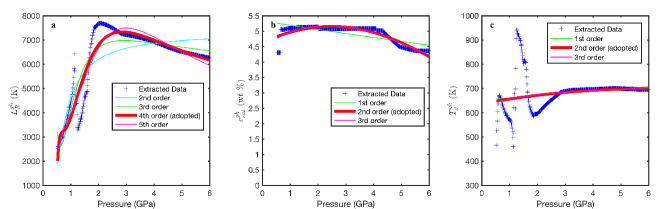
Figure 1: An example of fitting $L_{R}^{gh}$, $c_{sat}^{gh}$, and $T_{d}^{gh}$ of the gabbro–H₂O subsystem as polynomial functions of $1/P$ (a) and $P$ (b and c). The data used come from the PerpleX calculation of H₂O-saturated gabbro with oxide composition in Table 1. The thickened solid red lines denotes the polynomials adopted in this example case. Note that the fitting does not attempt to capture the wiggles of data around $\sim$1.2 GPa (a and c) because it will require extremely high-order polynomials and doesn’t gain much.

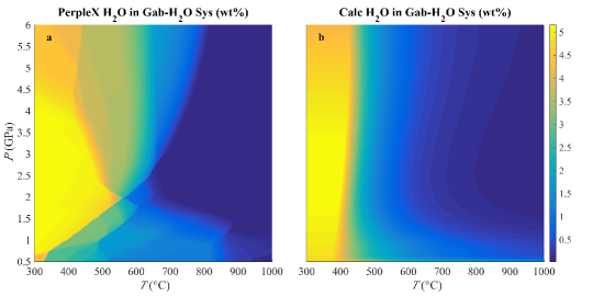
Figure 2: Comparison between the gabbro H₂O contents ($c_{s}^{\mathrm{H_{2}O}}$) derived from PerpleX (a) and our parameterization (b) for the gabbro–H₂O subsystem. “Gab” in the titles is short for gabbro, and the same as below.

By substituting equations (13)–(15) into (1) and noting that $c_{l}^{\mathrm{H_{2}O}}=1$ in the subsystem, the H₂O content in gabbro ($c_{s}^{\mathrm{H_{2}O}}$) is computed and plotted in Figure 2b for comparison with the PerpleX result in Figure 2a. It can be seen that the phase diagram from PerpleX contains multiple dehydration reactions diagnostic of both continuous and discontinuous reduction in the H₂O content of gabbro [1], whereas the parameterization is an average of these reactions. The effectively averaged reaction is characterized by an onset dehydration temperature ($T_{d}^{\mathrm{H_{2}O}}$), and a gradual H₂O content reduction the rate of which is controlled by $L_{R}$. Therefore, the parameterized $T_{d}^{\mathrm{H_{2}O}}$, $c_{sat}^{\mathrm{H_{2}O}}$, and $L_{R}$ capture the gross behavior of the subsystem with respect to initial dehydration, maximum H₂O content, and the smoothness of dehydration reaction. Experimental studies on MORB [27], which is compositionally similar to gabbro, show that below $\sim$2.2–2.4 GPa where amphiboles break down, there is a larger number of dehydration reactions than above $\sim$2.4 GPa, and this gives rise to a gradual reduction in gabbro H₂O content. Above this pressure, the varieties of hydrous phases reduce to dominantly lawsonites and phengites, leading to less dehydration reactions. Since phengites decomposition occurs at higher temperatures than lawsonites and principally participate in fluid-absent melting, the H₂O release above $\sim$2.2–2.4 GPa is mostly caused by lawsonite breakdown between $\sim$700–800 ^∘C. The reduction of gabbro H₂O content accordingly becomes sharper in this pressure range. These two features of dehydration under low and high pressure conditions are captured in Figure 2b of our parameterization.

III.1.2 Gabbro–CO₂ Subsystem

The same volatile-free bulk composition as in the gabbro–H₂O subsystem is used in the parameterization of the gabbro–CO₂ subsystem. Figure 3a illustrates the result of gabbro CO₂ content calculated by PerpleX under CO₂ saturation conditions. The same approach as above is used to extract $c_{sat}^{\mathrm{CO_{2}}}$, $L_{R}$, and $T_{d}^{\mathrm{CO_{2}}}$, and the following polynomials best fit the data extracted from PerpleX:

$$c_{sat}^{gc}(P)=a_{0},$$ (16)

$$\ln(L_{R}^{gc}(P))=b_{0}/P+b_{1},$$ (17)

$$T_{d}^{gc}(P)=c_{0}P+c_{1},$$ (18)

where the superscript “$gc$” represents “gabbro–CO₂”. Because the varieties of CO₂-bearing minerals are far less than those of hydrous minerals, the variation of saturated CO₂ content in the subsystem is minimal (Fig. 3a). In fact, the CO₂-containing minerals in Figure 3a are only aragonite, dolomite, and magnesite. Under CO₂ saturation conditions, it is thus the Mg and Ca content that determines the rock CO₂ content. Given that the Mg and Ca mass fractions in the bulk lithology are assumed to be constant, the $c_{sat}^{\mathrm{CO_{2}}}$ values are virtually unchanging. Vanishingly small variations of $c_{sat}^{\mathrm{CO_{2}}}$ occur in the PerpleX plot (Fig. 3a) due to minor variations of total amount of Mg and Ca (and sometimes Fe) that participates in carbonate formation. At a fixed pressure, the stable carbonate phase(s) change from aragonite to dolomite + magnesite, and to dolomite with increasing temperature. However, these mineralogical transformations involve mostly the adjustment of Ca and Mg proportions in the carbonates (solid solutions), rather than the total amount of Ca and Mg that forms carbonates. In consequence, the CO₂ content stays more or less constant until a temperature is reached where all the CO₂-bearing minerals become unstable, that is, the breakdown of dolomite. Beyond this temperature, no minerals can hold CO₂ and its content in gabbro sharply reduces to almost zero, as illustrated in Figure 3a. Our parameterization in Figure 3b captures this decarbonation feature, with a constant $c_{sat}^{\mathrm{CO_{2}}}$, a decarbonation curve $T_{d}^{\mathrm{CO_{2}}}(P)$ approximating dolomite breakdown, and large $L_{R}^{gc}(P)$ accounting for the sharp reduction of CO₂ beyond $T_{d}^{\mathrm{CO_{2}}}$. The regressed parameters are given in Table 2.

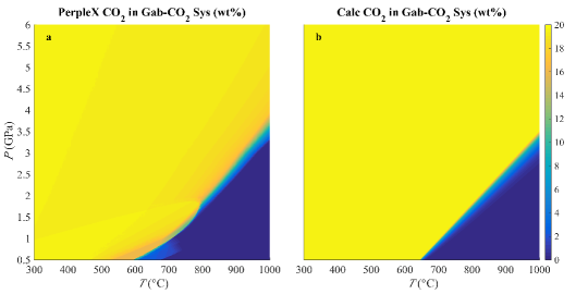
Figure 3: Comparison between the gabbro CO₂ contents ($c_{s}^{\mathrm{CO_{2}}}$) derived from PerpleX (a) and our parameterization (b) for the gabbro–CO₂ subsystem.

III.1.3 Gabbro–H₂O–CO₂ Full System

With the parameters acquired above, the subsystem partition coefficients ($K^{i}$) can be calculated according to equation (1), and a tentative full system pseudosection at specified $c_{blk}^{\mathrm{H_{2}O}}$ and $c_{blk}^{\mathrm{CO_{2}}}$ (Table 1) can be computed according to equations (3)–(4). Using the same bulk composition as input to PerpleX independently yields another pseudosection that differs from the one calculated by parameterization. Following the strategy in Section II, the discrepancies are used to parameterize analogous $W_{\mathrm{H_{2}O}}$ and $W_{\mathrm{CO_{2}}}$ (eq. (9)–(10)) as polynomial functions of pressure. After experimenting with polynomials of increasing order, we find the following best fit the data:

$$\ln(-W_{\mathrm{H_{2}O}})=d_{0}P^{4}+d_{1}P^{3}+d_{2}P^{2}+d_{3}P+d_{4},$$ (19)

$$\ln(-W_{\mathrm{CO_{2}}})=e_{0}P^{4}+e_{1}P^{3}+e_{2}P^{2}+e_{3}P+e_{4}.$$ (20)

Table 2 lists the relevant coefficients from data fitting. Figure 4 demonstrates that the fully parameterized thermodynamic calculation compares well with that from PerpleX. In particular, as shown in Figure 4c & e, pressure increase at a specific temperature stablizes carbonate minerals and makes coexisting liquid deficient in CO₂. Moreover, temperature increase at a fixed pressure leads to CO₂ enrichment in the equilibrated liquid phase. These two leading-order features during devolatilization are observed by Molina and Poli [23] and reflected in our parameterization (Fig. 4d & f).

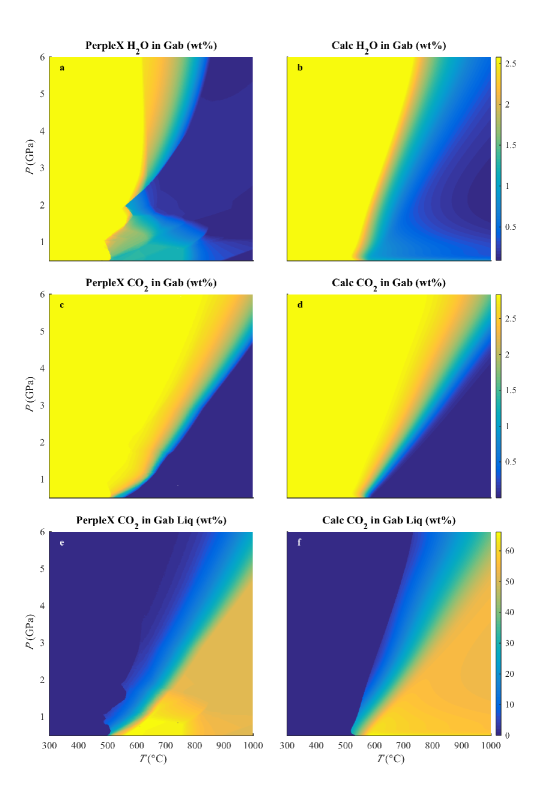
Figure 4: Comparison between the results from PerpleX (left panels) and our parameterization (right panels) for the gabbro–H₂O–CO₂ full system. Panels (a)–(b) are for H₂O content in solid rocks ($c_{s}^{\mathrm{H_{2}O}}$), (c)–(d) are for CO₂ content in solid rocks ($c_{s}^{\mathrm{CO_{2}}}$), and (e)–(f) are for CO₂ content in the liquid volatile phase ($c_{l}^{\mathrm{CO_{2}}}$). Note that $c_{l}^{\mathrm{H_{2}O}}=1-c_{l}^{\mathrm{CO_{2}}}$, so the comparability of H₂O content in the liquid phase can be deduced from that of CO₂.

Table 3: Regression Results for Gabbro–H₂O–CO₂ System

	H2O					CO2
$c_{sat}$	–	–	$-$0.0176673	0.0893044	1.52732	–	19.3795
$L_{R}$	$-$1.81745	7.67198	$-$10.8507	5.09329	8.14519	0.661119	10.9216
$T_{d}$	–	–	$-$1.72277	20.5898	637.517	118.286	857.854
$W_{\mathrm{H_{2}O}}$	–	–	$-$0.03522	0.5204	$-$2.381	3.64	$-$9.995
$W_{\mathrm{CO_{2}}}$	–	–	0.009474	$-$0.1576	0.9418	$-$2.283	13.37

III.2 Basalt Devolatilization

The same procedure as for gabbro is followed in parameterizing the MORB–CO₂–H₂O system, utilizing the volatile-free bulk composition for MORB from Table 1. Since all the data fitting in this contribution is in polynomial form, to avoid repetition, we detail the functional forms of parameterization for lithologies other than gabbro in Appendix B, and focus on discussing the parameterized results in the succeeding text.

A comparison between the parameterized and PerpleX results for the MORB–H₂O subsystem is illustrated in Figure 5. Considering that basalts and gabbros are compositionally close to each other, the phase diagrams in Figures 2a and 5a are much alike, and the fitting polynomials and plot from parameterization are accordingly similar. Therefore, the experimental validation of parameterization for gabbro devolatlization in Section III.1 applies to the representative basalts in this section.

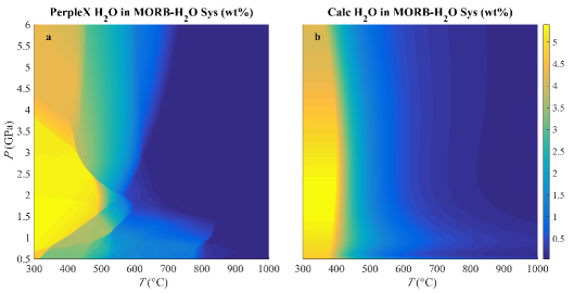
Figure 5: Comparison between the MORB H₂O contents ($c_{s}^{\mathrm{H_{2}O}}$) derived from PerpleX (a) and our parameterization (b) for the MORB–H₂O subsystem.

For the CO₂-only subsystem, Figure 6 compares the parameterization and PerpleX results. As noted in the instance for gabbro–CO₂ subsystem, due to the limited number of the varieties of carbonate minerals, the saturated CO₂ content ($c_{sat}^{\mathrm{CO_{2}}}$) is approximately constant, along with large $L_{R}$ values describing the sharp breakdown of the last carbonate mineral—dolomite.

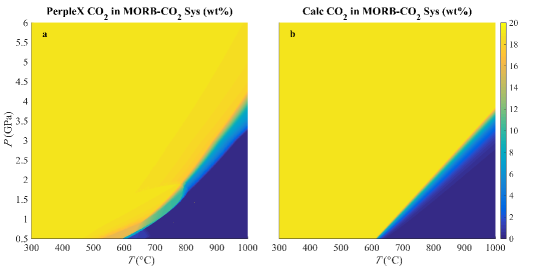
Figure 6: Comparison between the MORB CO₂ contents ($c_{s}^{\mathrm{CO_{2}}}$) derived from PerpleX (a) and our parameterization (b) for the MORB–CO₂ subsystem.

In synthesizing the subsystem parameterizations above to the full MORB–H₂O–CO₂ system, the bulk MORB composition in Table 1 is adopted in generating the PerpleX result which is further used when parameterizing the relevant $W_{\mathrm{H_{2}O}}$ and $W_{\mathrm{CO_{2}}}$. Polynomial forms for fitting the $W_{\mathrm{H_{2}O}}$ and $W_{\mathrm{CO_{2}}}$ data are provided in Appendix B. Figure 7 compares the the results from PerpleX and the parameterization for the full system. In addition to the two leading-order features outlined in Section III.1.3, comparison between Figure 7a and b shows that our parameterization favors H₂O release at low pressure and temperature conditions ($\sim$0.5–1.0 GPa and $\sim$500–700 ^∘C) relative to PerpleX. However, such a difference in low $P$ & $T$ regime does not affect modelling subduction-zone devolatilization because the global geotherms for the slab MORB layer all lie above this $P$ & $T$ region [e.g., Figure 5 in 7].

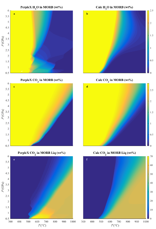
Figure 7: Comparison between the results from PerpleX (left panels) and our parameterization (right panels) for the MORB–H₂O–CO₂ full system. Panels (a)–(b) are for H₂O content in solid rocks ($c_{s}^{\mathrm{H_{2}O}}$), (c)–(d) are for CO₂ content in solid rocks ($c_{s}^{\mathrm{CO_{2}}}$), and (e)–(f) are for CO₂ content in the liquid volatile phase ($c_{l}^{\mathrm{CO_{2}}}$).

III.3 Sediment Devolatilization

Although sedimentary layers are only a few 100 m thick atop subducting slabs, they contain high abundance of incompatible minor and trace elements that are crucial in characterizing arc lava genesis [1]. As such, most experimental studies focus on the melting behavior of subducted sediments, rather than devolatilization [e.g., 28, 29, 30]. Our parameterization is thus compared below with previous modelling results and the limited experimental data available.

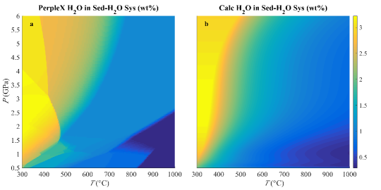
Figure 8: Comparison between the sediment H₂O contents ($c_{s}^{\mathrm{H_{2}O}}$) derived from PerpleX (a) and our parameterization (b) for the sediment–H₂O subsystem. “Sed” in the titles is short for sediment, and the same as below.

Figure 8 shows a comparison of the parameterized and PerpleX results for the sediment–H₂O subsystem. As hydrous mineral phases that can be stable in metapelites are abundant (e.g., micas, talc, chloritoid, chlorite, etc.), and they involve extensive solid solutions, the H₂O content changes smoothly. In addition, at pressures above $\sim$1.5 GPa, metapelite dehydration is dominated by the breakdown of two major hydrous phases—amphiboles and micas (Fig. 8a), so the parameterized initial dehydration curve $T_{d}^{sh}$ (see Appendix B) is approximately their average (Fig. 8b). Particularly, as Schmidt and Poli [1] inferred from the experiments by Chmielowski et al. [31], metapelite contains about 2.0 wt% H₂O at 3 GPa and 600 ^∘C, which is consistent with our parameterization in Figure 8b. However, in contrast to the PerpleX calculation, our parameterization does not predict complete dehydration at high temperatures ($>$ $\sim$900 ^∘C) and lower pressures ($<$ $\sim$2 GPa). Nonetheless, this limitation is unconcerning for the current parameterization because partial melting is expected in this $P$/$T$ range. Since both the parameterization and PerpleX calculation ignore partial melting, it is thus not necessary to match them in the $P$/$T$ region where partial melting would occur.

For the sediment–CO₂ subsystem, as the major carbonate phases in metapelites are still calcite/aragonite, magnesite, and dolomite [1], the formulae (see Appendix B) used during parameterization are the same as those for the basalt–CO₂ subsystem. A comparison of the PerpleX and parameterized results is illustrated in Figure 9, where the curve of the onset of decarbonation ($T_{d}^{sc}(P)$) approximates the breakdown of dolomite.

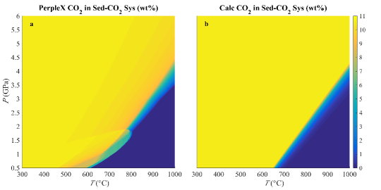
Figure 9: Comparison between the sediment CO₂ contents ($c_{s}^{\mathrm{CO_{2}}}$) derived from PerpleX (a) and our parameterization (b) for the sediment–CO₂ subsystem.

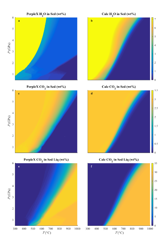
Figure 10: Comparison between the results from PerpleX (left panels) and our parameterization (right panels) for the sediment–H₂O–CO₂ full system. Panels (a)–(b) are for H₂O content in solid rocks ($c_{s}^{\mathrm{H_{2}O}}$), (c)–(d) are for CO₂ content in solid rocks ($c_{s}^{\mathrm{CO_{2}}}$), and (e)–(f) are for CO₂ content in the liquid volatile phase ($c_{l}^{\mathrm{CO_{2}}}$).

Figure 10 shows the parameterized results for the full sediment–H₂O–CO₂ system. Comparison of Figure 8b and 10b suggests that addition of carbonates into the system facilitates complete H₂O release at high temperatures. Close inspection of the PerpleX result in Figure 10a reveals that there are two major discontinuities in H₂O loss: one from H₂O content 7.2 wt% to $\sim$1 wt%, and the other from $\sim$1 wt% to almost 0 wt%. On the other hand, our parameterized result in Figure 10b depicts a gradual reduction of H₂O content from 7.2 wt% to almost 0 wt%. In addition, the parameterized onset temperature of H₂O loss is slightly higher than that from PerpleX, but the temperature of complete H₂O loss is lower for the parameterization than for PerpleX, which is consistent with the formalism adopted to effectively average devolatilization reactions (Appendix A). Further, comparison between Figure 9b and 10d suggests that addition of H₂O into the CO₂-only subsystem reduces decarbonation temperatures and thus promotes CO₂ release, facilitating the scenario of infiltration-driven decarbonation [4]. At 750–850 ^∘C and $\sim$2 GPa, experimental studies yield $X_{\mathrm{CO_{2}}}$ (mole fraction of CO₂ in liquid phase) estimates of 0.14 and 0.10–0.19 equilibrated with carbonated pelites and basalts respectively [23, 32]. Since $X_{\mathrm{CO_{2}}}\approx$ 0.14 converts to $\sim$28 wt% of CO₂, our parameterization illustrated in Figure 10f is compatible with these experimental constraints. Overall, with increasing temperature and decreasing pressure, Figure 10f shows that the equilibrated liquid phase becomes more and more CO₂-rich [32].

III.4 Devolatilization of Peridotite in Upper Mantle

Dehydration of hydrated slab mantle has been invoked as a mechanism for CO₂ release via infiltration-driven decarbonation [e.g., 4, 33]; moreover, the seismic activities within double seismic zones are also attributed to dehydration embrittlement in the slab upper mantle [e.g., 34]. Inferred from seismic data, the hydration state of the slab lithospheric mantle is highly variable and thus uncertain [see 35, 36], and the carbonation state even more so [e.g., 37]. Therefore, for the purpose of modelling slab devolatilization, the basal lithospheric mantle layer is treated as a water supplier that gives rise to H₂O infiltration into the overlying lithologies, and parameterization is performed on the H₂O-only subsystem.

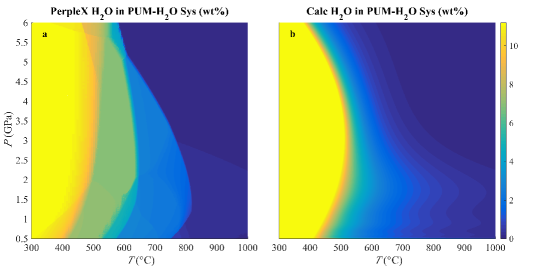
Figure 11: Comparison between the peridotite H₂O contents ($c_{s}^{\mathrm{H_{2}O}}$) derived from PerpleX (a) and our parameterization (b) for the peridotite–H₂O subsystem. “PUM” in the titles is short for peridotite in the upper mantle, and the same as below.

The volatile-free bulk composition for representative upper mantle is adopted from Hart and Zindler [38] and provided in Table 1. This composition is similar to the one for depleted mantle in Hacker [6], and is thus used for slab upper mantle composition residual to partial melting. The water content of this peridotite under H₂O-saturated condition is calculated by PerpleX and presented in Figure 11a. It is evident that there are three major dehydration reactions taking place with increasing temperature—breakdown of brucite, serpentine, and chlorite. Our parameterized result shown in Figure 11b captures the overall behavior of peridotite dehydration: the onset temperature of dehydration ($T_{d}^{ph}$) between $\sim$400–550 ^∘C approximates that of brucite decomposition; dewatering is more gradual at lower pressures ($<$ $\sim$3.5 GPa) because the three major dehydration reactions are more separated in temperature. Details of the parameterization are provided in Appendix B.

IV Simple Applications—Open System Effects

The parameterization performed above serves as a computational module that is interfaceable with reactive fluid flow modelling, under the assumption that local equilibrium holds during fluid–rock interaction (as in our companion paper, Part II). Although it ignores the details of specific dehydration and decarbonation reactions, the overall features of representative slab lithologies are captured. For example, released volatiles are H₂O rich close to the onset of devolatilization; more CO₂ comes into liquid phase with increasing temperature [23]. Since fluid flow renders the volatile-bearing system open, modelling of it entails thermodynamic computation that can accept evolving bulk composition and return the equilibrated thermodynamic state. Our parameterization meets this demand while being computationally efficient, and can thus simulate important open-system scenarios without needing repeated access to thermodynamic software (e.g. PerpleX) outside fluid flow models. To demonstrate this, we present its application to the two major open-system effects below.

IV.1 Effects of Fluid Removal (Fractionation)

In open systems, the released H₂O and/or CO₂ will migrate through the system due to buoyancy and other forces, desiccating formerly volatile-bearing rocks. Differential H₂O and CO₂ loss will alter the H₂O/CO₂ ratio in rock residues, giving rise to chemical fractionation. Consider an extreme case where H₂O is preferentially lost from a gabbro such that the residual volatile species is only CO₂. The system evolves to the CO₂-only subsystem as in section III.1.2. As demonstrated earlier, the onset temperatures of decarbonation are higher than those of dehydration. Therefore chemical fractionation will lead to elevated onset temperatures of devolatilization and inhibit further volatile loss.

An example is given in Figure 12a, where the white dashed line denotes the onset temperature of devolatlization for a representative gabbro containing 2.58 wt% H₂O and 2.84 wt% CO₂ (see Fig. 4f). At 780 ^∘C and 3.25 GPa (star symbol in Fig. 12a), this bulk composition yields the equilibrated porosity $\mathrm{9.1\times 10^{-2}}$ and liquid phase CO₂ mass fraction 0.36. The porosity level is equivalent to a liquid phase mass fraction $f=\mathrm{3.23\times 10^{-2}}$, if densities of liquid and solid are taken to be 1000 kg m^-3 and 3000 kg m^-3, respectively. For illustrative purposes, assuming that half of the liquid phase leaves the bulk system due to fluid flow, then the renormalized bulk volatile content is:

$$c^{i^{\prime}}_{blk}=\frac{c^{i}_{blk}-0.5fc^{i}_{l}}{1-0.5f},$$ (21)

where $i$ represents either H₂O or CO₂, and prime indicates renormalized values. The bulk H₂O content of 1.57 wt% and CO₂ content of 2.30 wt% after fractionation can be calculated from equation (21). Figure 12a shows the new equilibration with the renormalized bulk volatile content, where the red line marks the new onset temperatures of devolatilization. It is evident that the chemical fractionation causes elevation of the onset temperatures of devolatilization. At 780 ^∘C and 3.25 GPa, the newly equilibrated porosity is $\mathrm{2.4\times 10^{-2}}$ and liquid phase CO₂ mass fraction is 0.26, both lower than the pre-fractionation levels, demonstrating the increased difficulty in devolatilization, especially decarbonation.

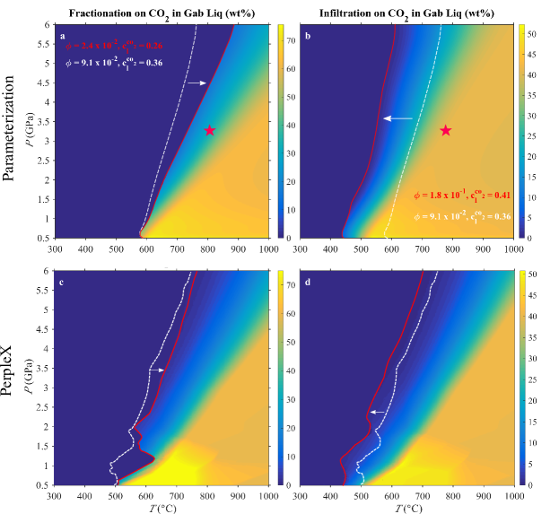
Figure 12: Illustration of the effects of fractionation (a and c) and infiltration (b and d). The upper panels show the results from our parameterization, whereas the lower panels show those from PerpleX, all based on the same bulk H₂O and CO₂ contents as detailed below. “Gab liq” in the titles denote liquid phase equilibrated with gabbro. The white dashed lines depict the onset of devolatilization for the reference case of full gabbro–H₂O–CO₂ system with 2.58 wt% bulk H₂O and 2.84 wt% bulk CO₂ (section III.1.3). Red solid lines denote the onset of devolatilization after bulk H₂O & CO₂ alterations by fractionation (panels a and c; with $c_{blk}^{\mathrm{H_{2}O}}$ = 1.57 wt% and $c_{blk}^{\mathrm{CO_{2}}}$ = 2.30 wt%) and by infiltration (panels b and d; with $c_{blk}^{\mathrm{H_{2}O}}$ = 4.13 wt% and $c_{blk}^{\mathrm{CO_{2}}}$ = 2.79 wt%). White arrows show the shift of onset temperatures from the reference case. Red stars mark the example pressure and temperature conditions used for comparison (see text). The corresponding porosity level and CO₂ weight fraction in liquid phase are given in the annotations.

IV.2 Effects of Fluid Addition (Infiltration)

Infiltration-driven decarbonation has been invoked as a potential mechanism of leaching CO₂ from subducting slabs to mantle wedge [e.g., 39]. When H₂O-rich fluids infiltrate porous rocks, the pore fluid that was in equilibrium becomes diluted in terms of CO₂ concentration and thus out of equilibrium. To restore fluid–rock equilibrium, the rock will release CO₂ into the liquid phase to counterbalance the dilution. As infiltration proceeds, CO₂ is constantly lost from rocks, giving rise to infiltration-driven decarbonation. This idealized scenario obscures one subtlety associated with fluid infiltration—a process that is, to some extent, reverse to the fractionation discussed in the previous section.

We highlight this subtlety through the following example. When a gabbroic rock is infiltrated by H₂O-rich fluids, the extra H₂O not only dilutes CO₂ in pore fluids, but also raises the bulk H₂O content in the fluid–rock system. Re-equilibration at elevated bulk H₂O content hence attempts not only to relieve the dilution via decarbonation reactions, but also to increase the fraction of coexisting liquid phase (i.e., porosity). Consider an extreme case where the infiltrating fluids are purely H₂O (e.g., from serpentinites), and the amount of added fluids is half that in the reference case of gabbro with 2.58 wt% bulk H₂O and 2.84 wt% CO₂. At 780 ^∘C and 3.25 GPa (red star in Fig. 12b), the coexisting liquid mass fraction before infiltration is $f=\mathrm{3.23\times 10^{-2}}$, so the bulk volatile content after infiltration can be calculated by:

$$c^{i^{\prime}}_{blk}=\frac{c^{i}_{blk}+0.5fc^{i}_{l}}{1+0.5f},$$ (22)

where $i$ represents either H₂O or CO₂, and prime indicates renormalized values. With $c^{\mathrm{H_{2}O}}_{l}=1$ and $c^{\mathrm{CO_{2}}}_{l}=0$ for pure H₂O infiltration, the renormalized values are thus 4.13 wt% bulk H₂O and 2.79 wt% bulk CO₂ after infiltration. Figure 12b shows the CO₂ mass fraction in the liquid phase under the new equilibration. The white dashed line marks the onset of devolatilization before infiltration (same as in Fig. 12a), whereas the red solid line marks that after infiltration. It is clear that the elevated bulk H₂O content caused by infiltration shifts the onset of devolatilization to lower temperatures. Thus, when temperature and pressure are fixed, such a shift can enhance the extent of devolatilization. In particular, at 780 ^∘C and 3.25 GPa (red star in Fig. 12b), the infiltration not only raises porosity from $\mathrm{9.1\times 10^{-2}}$ to $\mathrm{1.8\times 10^{-1}}$, but also increases the liquid phase CO₂ content from 36 wt% to 41 wt%. Therefore, the potential of H₂O infiltration in driving decarbonation comes not only from dilution of coexisting liquid phase, but also from the increase of devolatilization extent.

Figure 12c–d shows PerpleX calculations of the fractionation and infiltration effects in comparison with calculations using our parameterization (Fig. 12a–b). In general, the shift of devolatilization onset temperatures is bigger in our parameterized results than in the PerpleX ones. For fractionation, the shift in the parameterization (Fig. 12a) is up to 50 ^∘C higher than that in the PerpleX calculation (Fig. 12c) above $\sim$3.5 GPa, but it decreases below $\sim$3.5 GPa. For infiltration, the $\sim$50 ^∘C reduction in the shift of devolatilization onset temperatures (Fig. 12b & d) is virtually constant throughout the entire pressure range considered. This disparity in the predicted fractionation and infiltration effects comes from the highly averaged treatment of the gabbro+H₂O subsystem. As shown in Figure 2, there is a difference in the dehydration onset temperatures ($T_{d}^{gh}$) between the parameterized and PerpleX results, but such a difference is negligible for the gabbro+CO₂ subsystem (Fig. 3). When parameterizing the full system according to equations (5)–(7), this difference in the subsystem $T_{d}^{gh}$ is inherited, leading to the disparity between the top and bottom panels in Figure 12.

V Discussion

The parameterization presented thus far can model open-system thermodynamic behaviors for a rock–H₂O–CO₂ system, where “rock” represents typical lithologies in subducting slabs, i.e., sediments, basalts, gabbros, and peridotites. For each rock type, the parameterization predicts that CO₂ is released from the solid phase at higher temperature and lower pressure than H₂O, in accordance with experimental observations. Additionally, as dehydration and decarbonation in respective subsystems take place at different temperatures, the relative amounts of H₂O and CO₂ in bulk rocks control the onset temperature of overall devolatilization. The parameterization quantifies this compositional effect. These features enable efficient simulation of fractionation and infiltration during fluid flow, without the need to reproduce the full thermodynamics of devolatilization (i.e., compositional change of each mineral phase). As such, our approach balances model capability and complexity. Of course this balance means that some limitations are introduced, as compared with, e.g., PerpleX.

The first limitation is that the parameterization deals with systems that are open only to H₂O and CO₂. The effects of transport of other major, minor, and trace elements are not considered in the parameterization. For example, potassium is mobile in the presence of aqueous fluids [see 9, for a review] and its loss can destablize phengite, a major H₂O-bearing mineral phase [40, 41], and therefore alter the H₂O partition coefficients (eq. (1)) in a fundamental way. Furthermore, as calcium and magnesium are the primary elements that stablize carbonates (e.g., calcite, magnesite), their mobilization can also considerably affect the CO₂ partition coefficients. In consequence, in the case of significant non-volatile element loss or gain [e.g. 42, 43], the accuracy of our parameterization deteriorates.

The second limitation of the current parameterization is the omission of partial melting. Given that sediments and basalts occupy the hottest region near slab surface and are more likely to melt, the limitation of our parameterization is associated with neglecting the partial melting of pelites and basalts, rather than gabbros or peridotites. Extensive experimental studies have been conducted to determine the solidus of carbonated pelites [e.g., 29, 44, 30, 45, 28] and carbonated basalts [e.g., 46, 47, 30, 45, 48]. Regarding carbonated pelites, Thomsen and Schmidt [29] determined the solidus to be 900 ^∘C to 1070 ^∘C at pressures from 2.4 to 5.0 GPa. In a subsequent experiment on a sample with similar H₂O and CO₂ content, Tsuno and Dasgupta [30] determined a melting temperature between 800 ^∘C and 850 ^∘C at 3.0 GPa. As reviewed by Mann and Schmidt [28], the wet solidus for pelites ranges from 745 ^∘C to 860 ^∘C at pressures from 3.0 to 4.5 GPa in the presence of CO₂, but the fluid-absent solidus is from 890 ^∘C to 1040 ^∘C. These studies suggest that carbonated silicate melting or carbonatite melting are unrealistic for subducting sediments due to the low slab geotherms, unless H₂O saturation is realized near the wet solidus of carbonated sediments. Hence, our current parameterization for sediment devolatilization is applicable to the scenarios where sediments are either H₂O undersaturated or H₂O saturated but at temperatures below the wet solidus. On the other hand, the solidus of carbonated basalts (eclogites) was investigated by Dasgupta et al. [48], Yaxley and Brey [46], and Tsuno and Dasgupta [47], and was shown to exceed the maximum temperatures that can be reached within subducting slabs. This supports our omission of basalt partial melting in the parameterization. Thus, neglect of partial melting in our parameterization is valid in most cases. In rare cases where slab melting occurs as inferred from surface adakitic magmatism [49], the current parameterization becomes inappropriate.

The third limitation is the overestimation of open-system effects caused by fluid removal and addition, as discussed in section IV. This limitation is inherent in our parameterization, and not relevant to PerpleX. Qualitatively, fractionation tends to inhibit devolatilization whereas infiltration tends to promote it. In terms of modelling coupled H₂O & CO₂ transport in subducting slabs, these effects are likely to counterbalance each other. Quantitatively, however, it is uncertain to what extent this counterbalance is effective. A future improvement might look for alternative functional forms other than the quadratic one (eq. (6)–(7)) to achieve better predictions of onset temperatures of devolatilization. Nevertheless, compared with the conventional approaches that are fully based on PerpleX but ignore open-system behaviors, the current parameterization allows efficient treatment of open-system behaviors. With the recent increasing recognition of carbon transport via dissolved ionic species in subduction zones [e.g., 50], open-system effects are thought to play a dominant role in carbon transport. Therefore, a thermodynamic model capable of dealing with fractionation and infiltration seems highly desirable. The parameterization approach would be particularly advantageous when ionic species are included; in particular, the first limitation above is overcome.

VI Conclusion

In light of considerable uncertainties regarding the spatio-temporal pattern of fluid flow and the equilibrium state in the downwelling slabs, a balance between model capability and complexity should be maintained when assessing the slab H₂O and CO₂ budget during subduction. We present a thermodynamic parameterization for the devolatilization of representative lithologies in slabs comprising sediments, basalts, gabbros, and peridotites. This parameterization achieves an appropriate balance in that it captures the leading-order features of coupled decarbonation and dehydration, while it smooths over the details of specific mineral reactions, either continuous or discontinuous. The first captured feature is that equilibrated fluids are increasingly CO₂-rich with elevating temperature and reducing pressure, and the second is that increasing the CO₂/H₂O ratio in bulk rocks increases onset temperatures of devolatilization and thus inhibits overall devolatilization. With these two features, the parameterization is able to simulate the two open-system behaviors that significantly affect slab H₂O and CO₂ transport: fractionation and infiltration. Nonetheless, the current parameterization is limited to the scenarios in which metasomatism does not considerably alter the bulk rock composition with regard to non-volatile elements and the subducting slab does not partially melt. Within these limits, the parameterization can be efficiently coupled to reactive fluid flow modelling for the study of slab H₂O and CO₂ budget during subduction, the results of which are presented in the companion paper Part II.

Appendix A Derivation of the Formalism for Parameterization

For volatile $i$ (H₂O or CO₂) that reaches equilibrated partition between solid and liquid phases:

$$\mu^{i}_{s}=\mu^{i}_{l},$$ (23)

namely, the chemical potential ($\mu$) of this volatile component are equal between the two phases. Expanding on the thermodynamic state of pure material of component $i$:

$$\mu^{i}_{s0}(P,T)+RT\ln a^{i}_{s}=\mu^{i}_{l0}(P,T)+RT\ln a^{i}_{l},$$ (24)

where $a^{i}_{s}$ and $a^{i}_{l}$ are the activity of component $i$ in solid and liquid phases, respectively, and the subscript “$0$” denotes the chemical potential of pure material. Equation (24) can be rearranged as:

$$\ln\frac{a^{i}_{s}}{a^{i}_{l}}=\frac{1}{RT}\left[\mu^{i}_{l0}(P,T)-\mu^{i}_{s0}(P,T)\right],$$ (25)

where the right hand side is a function of only pressure ($P$) and temperature ($T$), not composition. In the ideal solution theory, dissolution of other components has no effects on the component $i$, indicating that the activity ratio of $a^{i}_{s}$ over $a^{i}_{l}$ is approximately that of respective concentrations ($c$), namely:

$$\ln\frac{a^{i}_{s}}{a^{i}_{l}}\approx\ln\frac{c^{i}_{s}}{c^{i}_{l}}=\ln K^{i},$$ (26)

where $K^{i}$ is the partition coefficient of component $i$. In the case of non-ideal solution, we have:

$$\ln\frac{a^{i}_{s}}{a^{i}_{l}}=\ln\frac{\gamma^{i}_{s}c^{i}_{s}}{\gamma^{i}_{l}c^{i}_{l}},$$ (27)

where $\gamma^{i}_{s}$ and $\gamma^{i}_{l}$ are the activity coefficients for component $i$ in solid and liquid phases, respectively. If it is further assumed that volatile concentrations in solid phase ($c^{i}_{s}$) is small such that Henry’s Law of dilute solution applies,

$$\ln\frac{a^{i}_{s}}{a^{i}_{l}}=\ln\frac{\gamma_{0}c^{i}_{s}}{\gamma^{i}_{l}c^{i}_{l}}=\ln\frac{K^{i}}{\gamma^{i}},$$ (28)

where $\gamma^{i}=\gamma^{i}_{l}/\gamma_{0}$, and $\gamma_{0}$ is a constant according to Henry’s Law.

The right hand side of equation (25) can be transformed to:

$$\frac{1}{RT}\left[\mu^{i}_{l0}(P,T)-\mu^{i}_{s0}(P,T)\right]=\frac{1}{RT}\left[\Delta H(P,T)-T\Delta S(P,T)\right],$$ (29)

where $\Delta H$ and $\Delta S$ are the enthalpy and entropy changes associated with an effective reaction—the reaction that involves the conversion from solid to liquid state for material consisted of purely component $i$. Within the pressure and temperature range a subducting slab undergoes, there are multiple dehydration or decarbonation reactions. If we approximate $\Delta H$ and $\Delta S$ by their average values corresponding to the multiple reactions ($\Delta H$ and $\Delta S$ represent respectively the enthalpy and entropy changes of an effectively averaged dehydration ($i=\mathrm{H_{2}O}$) or decarbonation ($i=\mathrm{CO_{2}}$) reaction), then

$$\Delta H(P,T)\approx\Delta H^{i}(P)=T^{i}_{d}(P)\Delta S^{i}(P)\approx T^{i}_{d}(P)\Delta S(P,T),$$ (30)

where $T^{i}_{d}(P)$ is the onset temperature of the averaged dehydration or decarbonation. Note that since the onset of average reaction is univariant and corresponds to a line in $P$-$T$ space, that is, $\Delta H^{i}(T_{d}^{i},P)=\Delta H^{i}(T_{d}^{i}(P),P)=\Delta H^{i}(P)$ and similarly for $\Delta S^{i}(T_{d}^{i},P)$, the $\Delta H^{i}$ and $\Delta S^{i}$ in equation (30) are written as pressure dependent only. Substituting equation (30) into equation (29), we get:

$$\frac{1}{RT}\left[\mu^{i}_{l0}(P,T)-\mu^{i}_{s0}(P,T)\right]\approx\frac{\Delta H^{i}(P)}{R}\left[\frac{1}{T}-\frac{1}{T^{i}_{d}}\right].$$ (31)

To conclude, for ideal solutions, equations (25), (26) and (31) lead to:

$$K^{i}\approx\exp\left[\frac{\Delta H^{i}(P)}{R}\left(\frac{1}{T}-\frac{1}{T^{i}_{d}}\right)\right],$$ (32)

whereas for non-ideal solutions, equations (25), (28) and (31) lead to:

$$\frac{K^{i}}{\gamma^{i}}\approx\exp\left[\frac{\Delta H^{i}(P)}{R}\left(\frac{1}{T}-\frac{1}{T^{i}_{d}}\right)\right].$$ (33)

Let $L_{R}(P)=\Delta H^{i}(P)/R$ and adopt $\mathcal{K}^{i}$ for the partition coefficients in the non-ideal cases:

$$K^{i}\approx\exp\left[L_{R}\left(\frac{1}{T}-\frac{1}{T^{i}_{d}}\right)\right],$$ (34)

$$\mathcal{K}^{i}\approx\gamma^{i}\exp\left[L_{R}\left(\frac{1}{T}-\frac{1}{T^{i}_{d}}\right)\right].$$ (35)

If a common factor of saturation content $c^{i}_{sat}$ is further singled out from equations (34) and (35), then the formalism of equations (1) and (8) respectively in the main text is recovered.

Appendix B Polynomials Fitted in the Parameterization

B.1 MORB

B.1.1 MORB–H₂O Subsystem

For the MORB–H₂O subsystem, we found the following polynomials best fit the PerpleX-derived data:

$$\ln(c_{sat}^{mh}(P))=a_{0}P^{3}+a_{1}P^{2}+a_{2}P+a_{3},$$ (36)

$$\ln(L_{R}^{mh}(P))=b_{0}/P^{4}+b_{1}/P^{3}+b_{2}/P^{2}+b_{3}/P+b_{4},$$ (37)

$$T_{d}^{mh}(P)=c_{0}P^{2}+c_{1}P+c_{2},$$ (38)

and the polynomial coefficients are provided in Table 4.

Table 4: Regression Results for MORB–H₂O–CO₂ System

	H2O						CO2
$c_{sat}$	–	–	0.0102725	$-$0.115390	0.324452	1.41588	–	19.0456
$L_{R}$	–	$-$1.78177	7.50871	$-$10.4840	5.19725	7.96365	0.505130	10.6010
$T_{d}$	–	–	–	$-$3.81280	22.7809	638.049	116.081	826.222
$W_{\mathrm{H_{2}O}}$	–	–	–	$-$0.05546	0.8003	$-$3.595	5.155	10.02
$W_{\mathrm{CO_{2}}}$	$-$0.001217	0.03207	$-$0.3466	1.98	$-$6.419	11.75	$-$11.08	15.06

B.1.2 MORB–CO₂ Subsystem

Similar to the gabbro–CO₂ subsystem, we found the following polynomials best fit the PerpleX-derived data of the MORB–CO₂ subsystem:

$$c_{sat}^{mc}(P)=a_{0},$$ (39)

$$\ln(L_{R}^{mc}(P))=b_{0}/P+b_{1},$$ (40)

$$T_{d}^{mc}(P)=c_{0}P+c_{1},$$ (41)

where values of coefficients are listed in Table 4.

B.1.3 MORB–H₂O–CO₂ Full System

In fitting the data of $W_{\mathrm{H_{2}O}}$ and $W_{\mathrm{CO_{2}}}$ derived from calibrating against PerpleX calculation, we experiment with polynomials of pressure from low to high orders, and the following forms turn out to best fit the data:

$$\ln(-W_{\mathrm{H_{2}O}})=d_{0}P^{4}+d_{1}P^{3}+d_{2}P^{2}+d_{3}P+d_{4},$$ (42)

$$\ln(-W_{\mathrm{CO_{2}}})=e_{0}P^{7}+e_{1}P^{6}+e_{2}P^{5}+e_{3}P^{4}+e_{4}P^{3}+e_{5}P^{2}+e_{6}P+e_{7}.$$ (43)

The fitted coefficients are provided in Table 4. For fitting of polynomials higher than the fifth order (e.g., equation (43)), we illustrate the quality of regression in Figure 13, which additionally includes those for equations (45) and (53).

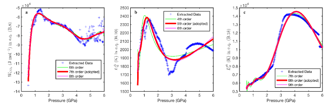
Figure 13: Illustration for the quality of high-order polynomial fitting for $W_{CO_{2}}$, $L_{R}^{sh}$, and $L_{R}^{ph}$ from equations (43), (45), and (53), respectively. The thickened solid red lines denotes the polynomials adopted.

B.2 Sediment

B.2.1 Sediment–H₂O Subsystem

For the H₂O-only subsystem, using the volatile-free bulk composition for sediments in Table 1, values of $c_{sat}^{\mathrm{H_{2}O}}$, $L_{R}$, and $T_{d}^{\mathrm{H_{2}O}}$ can be extracted from a PerpleX run assuming H₂O saturation. The following polynomial forms of pressure turn out to best fit the PerpleX-derived data, and the fitted coefficients are provided in Table 5.

$$\ln(c_{sat}^{sh}(P))=a_{0}(\log P)^{2}+a_{1}(\log P)+a_{2},$$ (44)

$$\ln(L_{R}^{sh}(P))=b_{0}/P^{5}+b_{1}/P^{4}+b_{2}/P^{3}+b_{3}/P^{2}+b_{4}/P+b_{5},$$ (45)

$$T_{d}^{sh}(P)=c_{0}P^{3}+c_{1}P^{2}+c_{2}P+c_{3}.$$ (46)

Table 5: Regression Results for Sediment–H₂O–CO₂ System

	H2O						CO2
$c_{sat}$	–	–	–	$-$0.150662	0.301807	1.01867	–	10.5923
$L_{R}$	$-$2.03283	10.8186	$-$21.2119	18.3351	$-$6.48711	8.32459	0.0974525	10.9734
$T_{d}$	–	–	2.83277	$-$24.7593	85.9090	524.898	92.5788	874.392
$W_{\mathrm{H_{2}O}}$	–	–	–	–	–	–	0.1045	12.53
$W_{\mathrm{CO_{2}}}$	–	–	–	–	–	–	–	$-\mathrm{10^{4}}$

B.2.2 Sediment–CO₂ Subsystem

Due to the limited varieties of carbonate mineral phases, the polynomial forms used for fitting the sediment–CO₂ subsystem are the same as in earlier subsystems:

$$c_{sat}^{sc}(P)=a_{0},$$ (47)

$$\ln(L_{R}^{sc}(P))=b_{0}/P+b_{1},$$ (48)

$$T_{d}^{sc}(P)=c_{0}P+c_{1},$$ (49)

where the fitted coefficients are listed in Table 5.

B.2.3 Sediment–H₂O–CO₂ Full System

In the full sediment–H₂O–CO₂ system, we found the following polynomials fitted for $W_{\mathrm{H_{2}O}}$ and $W_{\mathrm{CO_{2}}}$ best reproduce the result from PerpleX calculation, and the coefficients are listed in Table 5.

$$\ln(-W_{\mathrm{H_{2}O}})=d_{0}P+d_{1},$$ (50)

$$\ln(-W_{\mathrm{CO_{2}}})=e_{0}.$$ (51)

Table 6: Regression Results for Peridotite–H₂O Subsystem

	H2O
$c_{sat}$	–	–	–	–	–	–	–	0.00115628	2.42179
$L_{R}$	$-$19.0609	168.983	$-$630.032	1281.84	$-$1543.14	1111.88	$-$459.142	95.4143	1.97246
$T_{d}$	–	–	–	–	–	–	$-$15.4627	94.9716	636.603

B.3 Peridotite of Upper Mantle

The same procedure as for other subsystems is adopted to derive $c_{sat}^{\mathrm{H_{2}O}}$, $T_{d}^{\mathrm{H_{2}O}}$, and $L_{R}$ from PerpleX using the volatile-free bulk composition for peridotite (Table 1). In fitting the data as polynomial functions of pressure, we found the following achieve the best fit:

$$\ln(c_{sat}^{ph}(P))=a_{0}P+a_{1},$$ (52)

$$\ln(L_{R}^{ph}(P))=b_{0}/P^{8}+b_{1}/P^{7}+b_{2}/P^{6}+b_{3}/P^{5}+b_{4}/P^{4}+b_{5}/P^{3}+b_{6}/P^{2}+b_{7}/P+b_{8},$$ (53)

$$T_{d}^{ph}(P)=c_{0}P^{2}+c_{1}P+c_{2}.$$ (54)

Regressed coefficients are listed in Table 6 and comparison between PerpleX and the parameterization is given in Figure 11. Note that equation (53) is 8th order in $P^{-1}$, this does not collapse our parameterization at high peressures because $P^{-1}$ turns negligibly small and it is the lower-order terms that matter. Nonetheless, these high-order terms are retained to fine-tune the variation of dehydration rate under low pressure conditions, as reflected by the variation of H₂O content with temperature below $\sim$2.5 GPa in Figure 11a.