Multiphase quasar-driven outflows in PG 1114+445

Substantial evidence in the last few decades suggests that outflows from supermassive black holes (SMBH) may play a significant role in the evolution of galaxies. These outflows, powered by active galactic nuclei (AGN), are thought to be the fundamental mechanism by which the SMBH transfers a significant fraction of its accretion energy to the surrounding environment. Large-scale outflows known as warm absorbers (WA) and fast disk winds known as ultra-fast outflows (UFO) are commonly found in the spectra of many Seyfert galaxies and quasars, and a correlation has been suggested between them. Recent detections of low ionization and low column density outflows, but with a high velocity comparable to UFOs, challenge such initial possible correlations. Observations of UFOs in AGN indicate that their energetics may be enough to have an impact on the interstellar medium (ISM). However, observational evidence of the interaction between the inner high-ionization outflow and the ISM is still missing. We present here the spectral analysis of 12 XMM-Newton/EPIC archival observations of the quasar PG 1114+445, aimed at studying the complex outflowing nature of its absorbers. Our analysis revealed the presence of three absorbing structures. We find a WA with velocity $v\sim 530$ km s^-1, ionization $\log\xi/\text{erg cm s}^{-1}\sim 0.35,$ and column density $\log N_{\text{H}}/\text{cm}^{-2}\sim 22$, and a UFO with $v_{\text{out}}\sim 0.145c$, $\log\xi/\text{erg cm s}^{-1}\sim 4$, and $\log N_{\text{H}}/\text{cm}^{-2}\sim 23$. We also find an additional absorber in the soft X-rays ($E<2$ keV) with velocity comparable to that of the UFO ($v_{\text{out}}\sim 0.120c$), but ionization ($\log\xi/\text{erg cm s}^{-1}\sim 0.5$) and column density ($\log N_{\text{H}}/\text{cm}^{-2}\sim 21.5$) comparable with those of the WA. The ionization, velocity, and variability of the three absorbers indicate an origin in a multiphase and multiscale outflow, consistent with entrainment of the clumpy ISM by an inner UFO moving at $\sim 15\%$ the speed of light, producing an entrained ultra-fast outflow (E-UFO).

1 Introduction

Supermassive black holes (SMBH) in active galactic nuclei (AGN) are thought to be fundamental players in the evolution of their host galaxies. This is evident since host-galaxy properties, such as the stellar velocity dispersion (e.g., Ferrarese & Merritt, 2000) and the mass of the bulge (e.g., Häring & Rix, 2004), are correlated with the black hole mass. This suggests the existence of a “feedback” mechanism between AGN activity and the star formation process, and disk winds are the most promising candidates to drive such processes (e.g., King & Pounds, 2015; Fiore et al., 2017).
Moderately ionized winds ($\xi\lesssim 100$ erg cm s^-1) are often detected in the soft X-ray band as blue-shifted absorption lines and edges, indicating that these so-called warm absorbers (WA) have velocities in the range $v\sim 100-1000$ km s^-1 (e.g., Halpern, 1984; Blustin et al., 2005; Kaastra et al., 2014). Another class of winds, detected through X-ray absorption in AGNs, known as ultra-fast outflows (UFOs), is characterized by a much higher ionization state ($\xi\sim 10^{3}-10^{6}$ erg cm s^-1) and velocity ($v\sim 0.1-0.4c$), measured through absorption lines of highly ionized gas, most often Fe XXV and Fe XXVI (e.g., Chartas et al., 2002; Pounds et al., 2003a, b; Tombesi et al., 2010a, b, 2011; Giustini et al., 2011; Gofford et al., 2013; Tombesi et al., 2014, 2015; Nardini et al., 2015; Vignali et al., 2015; Braito et al., 2018).
Tombesi et al. (2013) found that WA and UFO parameters show overall trends in a sample of 35 Seyfert galaxies and quasars. This may suggest that WAs and UFOs could be different phases of a large-scale outflow. In particular, UFOs are launched at relativistic velocities, probably from the inner parts of the accretion disk surrounding the central SMBH, while WAs are most likely located at larger distances. However, there have been recent detections of fast outflows also in the soft X-ray band (e.g., Gupta et al., 2013, 2015; Longinotti et al., 2015; Pounds et al., 2016; Reeves et al., 2016), with identification of highly blue-shifted K$\alpha$ lines of O VI and O VII, suggesting high velocity ($v\sim 0.1-0.2c$), but lower ionization states than typical UFOs.
UFOs are thought to have a significant impact on the interstellar medium (ISM) of their host galaxy. In fact, current models (e.g., King, 2003, 2005) predict that inner UFOs may shock the ISM, transferring their kinetic energy to the ambient medium and possibly driving feedback on their host galaxy. In the aftermath of the shock, such models predict four regions being formed: (i) the inner UFO, (ii) the shocked UFO, (iii) the shocked swept-up ISM, and (iv) the outer ambient medium, not yet affected by the inner outflows. If the hot shocked gas cools down effectively, which means that the cooling time is shorter than the flow time, only momentum is conserved. In the opposite case of negligible cooling, the energy is conserved and hence the UFO transfers its kinetic power to the ISM (e.g., Costa et al., 2014; King & Pounds, 2015), possibly clearing out the galaxy of its own gas (e.g., Zubovas & King, 2012). Even though direct evidence of the shocked ISM has been claimed in the past (Pounds & Vaughan, 2011), it has been recently proposed that the observed low-ionization UFOs are due to shocked ISM by the inner UFO (Sanfrutos et al., 2018).
In addition, Gaspari & Sa̧dowski (2017) have shown that galaxy evolution might be regulated by a duty cycle between such multiphase AGN feedback, and a feeding phase that is thought to be due to so-called chaotic cold accretion (CCA, Gaspari et al., 2013), which is the cooling of gas clumps and clouds that “rain” toward the innermost regions of the AGN (e.g., Gaspari et al., 2018). While observational evidence of the feedback phase has been extensively collected in the last two decades in many spectral rest-frame bands, such as X-rays, optical, UV, and sub-millimetric (see, e.g., Fiore et al., 2017; Cicone et al., 2018, for recent reviews), only recent observations are starting to detect the feeding phase (e.g., Tremblay et al., 2016; Lakhchaura et al., 2018; Tremblay et al., 2018; Temi et al., 2018).

PG 1114+445 is a type-1 quasar at $z=0.144$ (Hewett & Wild, 2010). The mass of the central SMBH and the bolometric luminosity are estimated (Shen et al., 2011) as $\log(M/M_{\odot})\sim 8.8$ and $\log(L_{\text{bol}}/\text{erg s}^{-1})\sim 45.7$, respectively, implying an Eddington ratio of $L/L_{\text{Edd}}\sim 7\%$. The source was observed in 1996 by the Advanced Satellite for Cosmology and Astrophysics (ASCA) in the X-ray band and by Hubble Space Telescope (HST) Faint Object Spectrograph (FOS) camera in the UV band. The X-ray analysis (George et al., 1997) showed the presence of an ionized WA in the soft band, interpreted as photoelectric absorption edges of O VII and O VIII. Moreover, a detection of a possible absorption line at $E=7.25^{+0.42}_{-0.48}$ keV was interpreted as being due to highly ionized iron, possibly suggesting the presence of a mildly relativistic outflow with $v\sim 0.1c$. The investigation of the UV spectrum (Mathur et al., 1998) discovered C IV and Ly$\alpha$ narrow absorption lines (NAL), with line-of-sight velocities of $v_{\text{out}}\sim 530\text{ km s}^{-1}$. Given the similar ionization state of the soft X-ray and UV absorption features, Mathur et al. (1998) concluded that they are likely to originate from the same material.
In 2002, a much higher quality X-ray spectrum was obtained by a $44$ks XMM-Newton observation. These data revealed the complex two-component nature of the WA (Ashton et al., 2004; Piconcelli et al., 2005). In a recent ensemble work on a sample of optically selected quasars in XMM-Newton archival data (Serafinelli et al., 2017), we used 11 additional archival spectra, also included in a recent study based on the two-corona model (Petrucci et al., 2018). Here we present a detailed spectral analysis of these data, together with a re-analysis of both the 2002 XMM-Newton and the 1996 ASCA observations, aimed at unveiling the multiphase nature of the outflows of PG 1114+445.
The article is structured as follows. Section 2 describes the data reduction techniques used for these spectra. We show the spectral analysis and results in Sect. 3. The distances of the absorbers are computed in Sect. 4, while the energetics of the wind is described in Sect. 5. We summarize and discuss the results in Sect. 6. Throughout the paper we have use the following cosmology: $H_{0}=70$ km s^-1 Mpc^-1, $\Omega_{\text{m}}=0.3$ and $\Omega_{\Lambda}=0.7$.

2 Observations and data reduction

XMM-Newton observed PG 1114+445 on twelve occasions between 2002 and 2010. In May 2002 it was observed for $\sim 44$ks (OBSID 0109080801). Then, a campaign of 11 observations was performed between 2010 May 19 and 2010 December 12 (sequential OBSIDs from 0651330101 to 0651331101), for a total duration of $\sim 380$ ks. Details on duration and exposure of the single observations are given in Table 3. We extracted the event lists of the European Photon Imaging Camera (EPIC) detectors, both pn and Metal Oxide Semi-conductor (MOS), with the standard System Analysis Software (SAS, version 16.0.0) tools epproc and emproc. All observations are affected by background particle flaring (e.g., De Luca & Molendi, 2004; Marelli et al., 2017) to different extents, particularly OBSIDs from 0651330201 to 0651330501 (see Table 3 for details). Therefore, we applied an appropriate filtering to remove the times affected by this effect. After checking that no pile-up (e.g., Ballet, 1999) correction was needed for any of these observations, we extracted the spectra by selecting a region in the CCD image of $40^{\prime\prime}$ radius around the source, and the background by extracting a source-free region of the same size. We generated response matrices and auxiliary response files using the SAS tools rmfgen and arfgen respectively. Finally, we grouped the spectra by allowing 50 counts for each spectral bin using specgroup, considering a minimum energy width of one fifth of the full width half-maximum (FWHM) resolution. XMM-Newton MOS1 and MOS2 spectra were combined to obtain a higher signal-to-noise ratio (S/N). We considered the $0.3-10$ keV band of each spectrum.
We reduced the Reflection Grating Spectrometer (RGS) spectra by using rgsproc, screening times with high particle background through the examination of the RGS light curves, and using rgsfilter and rgsspectrum to produce clean spectra. However, we could not perform a statistically meaningful analysis because, even combining all 24 RGS1 and RGS2 spectra together with rgscombine, we obtained a combined mean spectrum with insufficient S/N. We also analyzed the 150 ks 1996 ASCA observation (ID 7407200), for which we retrieved the already reduced data products from the Tartarus ASCA AGN database (Turner et al., 2001).
For simplicity, we gave each observation a simple identification code, where Obs. A represents the ASCA observation, Obs. 0 is the 2002 XMM-Newton observation, while Obs. 1 to Obs. 11 label the 2010 campaign observations (see Table 3). Finally, we grouped together Obs. 1 to 3, 4 to 5, and 8 to 9 in order to increase the count rates of the single observations, mostly due to severe background particle screening, in order to reach a level of S/N adequate for the spectral analysis.

3 Spectral analysis

3.1 Models

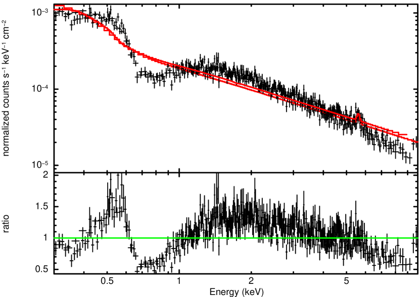
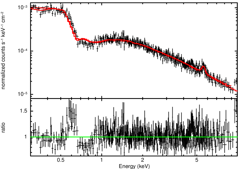
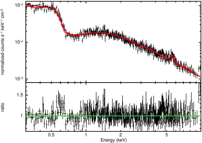
Figure 1: Spectral fits of EPIC-pn and EPIC-MOS1+2 data of Obs. 0. When only a continuum and blackbody model is included, the model poorly fits the data (top). We added an absorber, obtaining a significant improvement in the fit quality (middle). Our best fit model is obtained by adding a second absorber to the model (bottom).

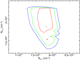
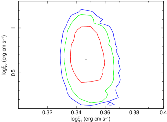
Figure 2: Contour plots of column density (left) and ionization parameter (right) of Absorber 1 versus Abs. 2 for Obs. 0. Red, green, and blue lines represent $68\%$, $90\%,$ and $95\%$ confidence levels, respectively. The black cross represents the best-fit values.

Figure 3: Contour plot of the observed redshift of Abs. 2, i.e. $z_{o,2}$ , versus the ionization $\log\xi_{2}$ for Obs. 0. Red, green, and blue lines represent $68\%$, $90\%,$ and $95\%$ confidence levels, respectively. The black cross represents the best-fit values.

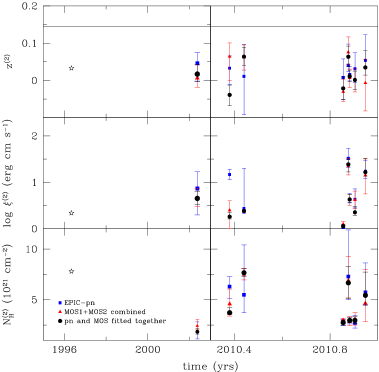
Figure 9: Best-fit values of the pn camera (blue squares), the MOS cameras combined (red triangles), and pn and MOS data together (black circles) of the three parameters of Abs. 2. The star is the ASCA value. The parameters are in agreement within their errors at $90\%$ confidence level. The horizontal black line represents the cosmological redshift of the source, $z_{o}=0.144$.

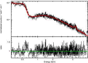
Figure 11: Spectrum and ratio of Obs. 0. The red line is the best fit.

The X-ray spectral analysis was carried out using the software XSPEC (Arnaud, 1996) included in the High-Energy Astrophysics SOFTware (HEASOFT) v6.18 software package. We fitted separately EPIC-pn and EPIC MOS1+2 spectra for each XMM-Newton observation, using a power law model with Galactic absorption, a soft excess modeled by a blackbody spectrum, and two ionized absorbers (named Absorber (Abs) 1 and Abs. 2), following indications from previous analyses of these spectra (Ashton et al., 2004; Piconcelli et al., 2005).
The best fit values of EPIC-pn and MOS spectra agree within a $90\%$ confidence level (see Figs. 9 and 10), therefore the results were recomputed fitting EPIC-pn and MOS spectra together, to obtain higher significance results. For the ASCA observation, we fitted together the spectra from all cameras of the telescope. Best-fit parameters of each spectra and the improvements in term of $\Delta\chi^{2}$ for each fit component are listed in Tables 4-7, while spectra and best-fit curves are shown in Figs. 11 to 18. In Fig. 1, we show the spectra and ratio of the continuum, continuum+Abs. 1, and continuum+Abs. 1+Abs. 2 models for Obs. 0.
We rule out instrumental artifacts or random fluctuations for the detection of Abs. 2 for the following reasons. First, the main spectral features are detected in the observed energy range $E=0.8-1.5$ keV, where no sharp edges are present in the effective area of both pn and MOS instruments. Second, if due to an instrumental artifact, the spectral features would have been detected at the same energy and with the same intensity in many other sources. Third, in case of instrumental artifact, we would not observe the same features in both pn and MOS within a $90\%$ confidence level for all the observations.
For three XMM-Newton observations, Obs. 1+2+3, Obs. 6, and Obs. 8+9, we also need a third absorber (Abs. 3) in the Fe K$\alpha$ band, associated with a UFO. In Table 6 we also report the best fit results for a third absorber in the ASCA observation, although it is found with significance below a $2\sigma$ confidence level threshold, in order to compare with the claim of George et al. (1997). We note that the detection probability of all the UFO reported in Table 6 is higher than $99\%$, even when considering a blind line search. In fact, extensive Monte Carlo simulations show that the null probability of a spectral feature in the $E=7-10$ keV band, with $\Delta\text{dof}=3$ (degrees of freedom), is $\sim 1\%$ for a $\Delta\chi^{2}\gtrsim 11$ (Tombesi et al., 2010a).
We modeled the ionized absorbers by computing detailed grids with the photoionization code XSTAR (Kallman & Bautista, 2001), which considers absorption lines and edges for every element with $Z\leq 30$. For Abs. 1 and 2, we calculated an XSTAR table with a spectral energy distribution in the $E=10^{-1}-10^{6}$ eV energy band described by a photon index of $\Gamma=2$, with cutoff energy beyond $E_{c}>100$ keV, following Haardt & Maraschi (1991). We considered standard solar abundances from Asplund et al. (2009) and turbulent velocity of $100$ km s^-1 (e.g., Laha et al., 2014). This value is well within the energy resolution provided by the EPIC-pn and MOS instruments, and testing different values did not provide statistically different results. Since Abs. 3 is associated with UFOs, we adopted a nearly identical model, with the only difference being a larger turbulent velocity, $v\sim 10^{3}$ km s^-1.
In the XSTAR grids, the free parameters are the absorber column density, $N_{\text{H}}$, its observed redshift, $z_{o}$, and the ionization parameter, $\xi=L_{\text{ion}}/r^{2}n,$ where $L_{\text{ion}}$ is the ionizing luminosity between $13.6$ eV and $13.6$ keV, computed by using the luminosity task in XSPEC on the unabsorbed best fit spectral model. The relation between the observed redshift $z_{o}$, the cosmological redshift $z_{c}$, and the Doppler shift $z_{a}$ of the absorber with respect to the source rest frame is

$$1+z_{o}=(1+z_{a})(1+z_{c}).$$

The velocity of the outflow is related to $z_{a}$ by the relation

$$1+z_{a}=\sqrt{\frac{1-v/c}{1+v/c}}.$$

In case of outflowing material, $z_{a}$ is a blueshift, and we conventionally adopt $v/c>0$.

3.2 Results

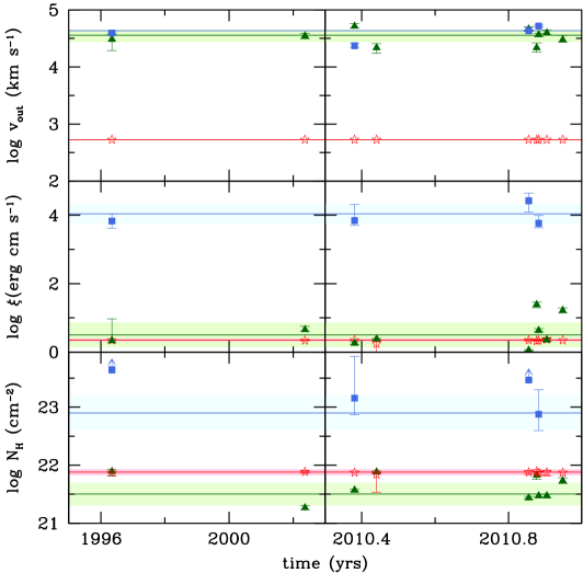
Figure 4: Time dependence of the outflow velocity $v_{\text{out}}$ (top), ionization parameter $\xi$ (middle), and column density $N_{\text{H}}$ (bottom). For each panel we show the values of Abs. 1 (red stars), Abs. 2 (green triangles), and Abs. 3 (blue squares). Lower limits on $N_{\text{H}}$ were marked with an arrow. Horizontal lines with shaded bands represent the median values and the corresponding median absolute deviations.

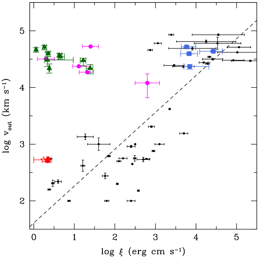
Figure 5: Velocity vs. ionization parameter plot for warm absorber (red stars), entrained ultra-fast outflow (green triangles), and ultra-fast outflow (blue squares). As expected, the UFO and the WA seem to follow a linear correlation. The smaller black points and the dashed line represent the points and the linear fit of Tombesi et al. (2013). The velocity of the WA constant to the value computed by Mathur et al. (1998) is $v\sim 530$ km s^-1. The E-UFO does not follow such a correlation. The magenta points represent other soft X-ray UFOs reported in the literature (see Sect. 1 for details).

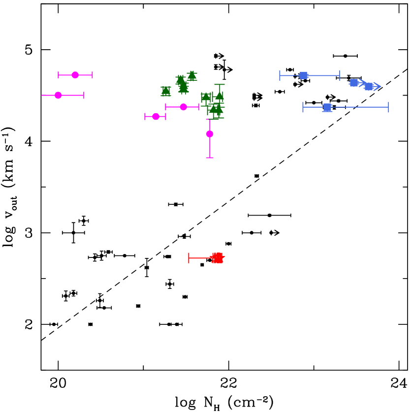
Figure 6: Velocity vs. column density plot for WA (red stars), E-UFO (green triangles), and UFO (blue squares). As in the case of Fig. 5, the warm absorber and the ultra-fast outflow are in agreement with Tombesi et al. (2013) (smaller black dots and dashed line). Arrows represent lower limits on $N_{\text{H}}$. Magenta points are soft X-ray UFOs in the literature. Again, the velocity of the warm absorber is assumed to be $v\sim 530$ km s^-1. Even though the green triangles do not follow the linear fit of Tombesi et al. (2013), there seems to be some continuity between the column density of this absorber and the ‘regular’ ultra-fast outflows.

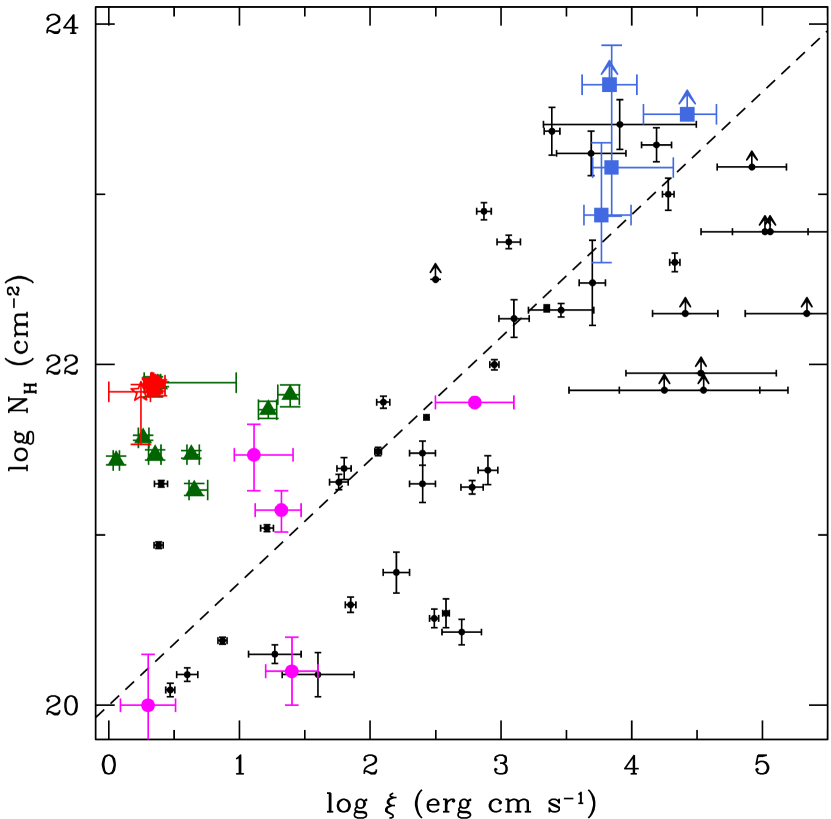
Figure 7: Column density vs. ionization parameter plot for WA (red stars), E-UFO (green triangles), and UFO (blue squares). Arrows represent lower limits on the column density, with the black dots and dashed line representing the linear fit from Tombesi et al. (2013). Magenta points are soft X-ray UFOs from the literature. This plot does not show any difference from Tombesi et al. (2013), since the E-UFO only differs from the WA in its velocity.

Absorber 1 shows a very low variability (see Table 4) in both ionization parameter $\log(\xi_{1}/\text{erg cm s}^{-1})=0.35\pm 0.04$ and column density $\log(N_{H,\text{1}}/\text{cm}^{-2})=21.88\pm 0.05$. The redshift of the absorber, mainly due to the shift of the Fe M-shell unresolved transition array (UTA), is comparable with the cosmological one of the source ($z_{o}=z_{c}$) within the EPIC energy resolution. In fact, when the absorber redshift is left free, the difference between the source redshift and the observed one is on the order of $\Delta z\sim 10^{-3}$, far below the energy resolution of the instrument. Therefore, its velocity is assumed to be fixed at $v_{1,\text{out}}\sim 530$ km s^-1, as shown by its corresponding absorption phase in the UV band (Mathur et al., 1998). These values of column density, velocity, and ionization are typical of a WA (Blustin et al., 2005).
Absorber 2 is more variable, as shown in Table 5, with median values for the ionization parameter and column density given by $\log(\xi_{2}/\text{erg cm s}^{-1})=0.50\pm 0.36$ and $\log(N_{\text{H},2}/\text{cm}^{-2})=21.5\pm 0.2$, respectively. We verified that the values of the parameters of Abs. 2 are independent from the ones of Abs. 1, ruling out any systematically induced correlation. In fact, even if the median values of the two absorbers are of the same order, the values of the individual observations are not correlated. Indeed, the correlation coefficient between non-fixed values of $N_{\text{H,1}}$ and the corresponding $N_{\text{H,2}}$ is $r=0.14$, while the one between $\log\xi_{1}$ and $\log\xi_{2}$ is $r=0.17$, showing that their variability is not related. Moreover, contour plots show no significant correlation between the column density and ionization parameter of Abs. 1 and Abs. 2 (see Fig. 2). The velocity of this absorber is measured with respect to the centroid energy of UTA Fe M and oxygen lines for the observations with lower ionization parameter, and the addition of Fe L lines for the observations with higher ionization parameter, such as Obs. 7 and 11 (see Table 5). Given the low resolution of the EPIC cameras, however, only Fe UTA are likely to contribute to the redshift calculation. As shown in Fig. 3, contour plots of the observed redshift $z_{o,2}$ and $\log\xi_{2}$ are well constrained. However, the observed redshift is below the systemic value $z_{c}=0.144$ even at $95\%$ confidence level. The median value of the velocity of this absorber is $v_{2,\text{out}}=(0.120\pm 0.029)c.$ Given the high velocity and low values of the ionization and column density, this absorber shows intermediate parameters between a WA and a UFO. In fact, outflows with $v\sim 0.1-0.4c$ are usually coupled with ionization parameters in the range $\log\xi/\text{erg\leavevmode\nobreak\ cm\leavevmode\nobreak\ s}^{-1}\sim 3-6$ (Tombesi et al., 2013), detectable by observing Fe XXV and XXVI absorption lines. The ionization parameter of this absorber is instead in the range $\log\xi_{2}/\text{erg\leavevmode\nobreak\ cm\leavevmode\nobreak\ s}^{-1}\sim 0-1.5$, much lower than the usual UFO and comparable with the range of ionization we find in WAs.
As mentioned, three observations show evidence of a third absorber. This absorber is variable (see Table 6) and the median values of column density, ionization, and velocity are respectively $\log(N_{H,\text{3}}/\text{cm}^{-2})=22.9\pm 0.3$, $\log(\xi_{3}/\text{erg cm s}^{-1})=4.04\pm 0.29,$ and $v_{3,\text{out}}=(0.140\pm 0.035)c$. These values are consistent with those of a typical UFO (e.g., Tombesi et al., 2011; King & Pounds, 2015). The median values of all the parameters of the three absorbers are summarized in Table 1, while the best-fit results of each absorber in time are shown in Fig. 4.
While the WA and the UFO agree with the linear trends in Tombesi et al. (2013) between column density, ionization parameter, and velocity, Abs. 2 does not fit well into such relations (see Fig. 5, 6, and 7) and it lies in a different region of the plots. It is straightforward to note that the velocity of Abs. 2 and that of the UFO are consistent within their dispersion, while $\xi$ and $N_{H}$ are consistent with those of the WA. This is a strong indication that this absorber is likely to be an intermediate phase between these two, possibly related to the interstellar medium being entrained by the UFO (see Sect. 5), and hence we can name this absorber the entrained ultra-fast outflow (E-UFO).

4 Distances of the absorbers

Table 1: Median values and median absolute deviation (MAD) for each parameter of three absorbers using the best-fit values of the XMM-Newton spectra.

Parameter	Median	Units
$\log N_{\text{H},1}$	$21.88\pm 0.05$	cm-2
$\log\xi_{1}$	$0.35\pm 0.04$	erg cm s-1
$v_{1,\text{out}}{*}$	$\sim 530$	km s-1
$\log N_{\text{H},2}$	$21.5\pm 0.2$	cm-2
$\log\xi_{2}$	$0.50\pm 0.36$	erg cm s-1
$v_{2,\text{out}}$	$0.120\pm 0.029$	$c$
$\log N_{\text{H},3}{**}$	$22.9\pm 0.3$	cm-2
$\log\xi_{3}$	$4.04\pm 0.29$	erg cm s-1
$v_{3,\text{out}}$	$0.145\pm 0.035$	$c$
$\log L_{\text{ion}}$	$45.4\pm 0.3$	erg s-1

Following Tombesi et al. (2013) and Crenshaw & Kraemer (2012) we can estimate the maximum distance of the absorber from the black hole, by assuming that the shell size is smaller than its distance from the center, meaning $N_{H}=nR<nr$, with $R$ size of the shell and $r$ distance from the SMBH, so that $n=N_{H}/r_{\text{max}}$. The determination of a well-defined ionization parameter indicates that we are observing a shell of gas with a thickness much smaller than the average distance of the absorber to the source, otherwise we would have detected a significantly larger gradient in the ionization parameter. Therefore we have

$$r_{\text{max}}=\frac{L_{\text{ion}}}{N_{\text{H}}\xi},$$ (1)

where $L_{\text{ion}}$ is the unabsorbed ionizing luminosity emitted by the source, for which we used the median value reported in Table 1.
We are also able to compute the minimum distance from the black hole, by computing the distance at which the observed velocity is equal to the escape velocity,

$$r_{\text{min}}=\frac{2GM_{\text{BH}}}{v_{\text{out}}^{2}}.$$ (2)

For the warm absorber, we obtain $r_{\text{min,WA}}\sim 10^{5}r_{s}\simeq 18$ pc and $r_{\text{max,WA}}\sim 10^{9}r_{s}\simeq 5\times 10^{5}$ pc, where $r_{s}=2GM_{\text{BH}}/c$ is the Schwarzschild radius. Since no constraints can be put on these values, we have to assume that the WA is located beyond $r_{\text{min,WA}}$. However, the external radius $r_{\text{max,WA}}$ is too extreme and therefore we do not report it on Table 2. We assume instead a typical value $r_{\text{max,WA}}\sim 3$ kpc (Di Gesu et al., 2013).
For the UFO, we obtain $r_{\text{min,UFO}}\sim 57r_{s}\simeq 3\times 10^{-3}$ pc and $r_{\text{max,UFO}}\sim 10^{4}r_{s}\simeq 0.5$ pc. Numerical simulations (e.g., Fukumura et al., 2015; Nomura et al., 2016; Sa̧dowski & Gaspari, 2017) show that the UFO launching region is confined within $r\lesssim 100r_{s}$ and therefore we conservatively assume $r_{\text{min,UFO}}$ as the typical value of the distance of the UFO from the central SMBH.
Having a UFO-like velocity, the minimum distance of the E-UFO from the central SMBH is much smaller than that of the WA, which is $r_{\text{min,E-UFO}}\sim 70r_{s}$. However, this value that is consistent with the distance of the UFO is not applicable, since a clumpy wind co-spatial with the UFO at $r<100r_{s}$ (e.g., Pounds et al., 2016) is excluded on the basis of photoionization considerations. In fact, the absorber would require a Compton-thick column density in order to be shielded from the intense radiation field and at the same time preserve its low ionization parameter. Moreover, the consistent values of both $N_{\text{H}}$ and $\xi$ between the WA and the E-UFO strongly suggest that the two absorbers share the same material, hence they are at comparable distances from the SMBH. Therefore, the E-UFO is most likely located in a shell with $r_{\text{min,E-UFO}}\gtrsim 18$ pc, in agreement with the location of the WA.
An alternative method to compute the distance of the absorber from the SMBH is to use the median absolute deviations (MAD) of $N_{\text{H}}$ and $v_{\text{out}}$ to estimate a typical value of the density of the absorber. Since a significant degree of clumpiness is expected for the ambient medium (e.g., Gaspari & Sa̧dowski, 2017), it is reasonable to assume that the variations of the typical shell radius $R$ are due to the velocity dispersion $\Delta v_{\text{out}}$. However, this is due to the fact that the shell’s apparent thickness depends on the peculiar clump we are observing, and it is not due to an intrinsic variability of the velocity and the physical properties of the gas in the clump.
To derive an estimate of the shell’s apparent thickness we consider $N_{\text{H}}\simeq nR$, and we can obtain through partial derivation

$$\frac{\Delta N_{\text{H}}}{\Delta t}=n\frac{\Delta R}{\Delta t}+R\frac{\Delta n}{\Delta t}.$$ (3)

We assume that in the time span of the XMM-Newton observations, $\Delta t\simeq 8.5$ yrs, the average density of the shell does not significantly vary, therefore $\Delta n/\Delta t\simeq 0$, and we assume that $\Delta R/\Delta t$ corresponds to the MAD of the velocity of the absorber, $\Delta v_{\text{out}}$. Given the variability of $N_{\text{H}}$ and $v_{\text{out}}$, we are able to compute a typical value of the shell density and consequently the distance of the absorber from the black hole, using the following equations:

$$\left<n\right>=\frac{\Delta N_{\text{H}}}{\Delta t\Delta v_{\text{out}}},$$ (4)

$$r_{\text{var}}=\sqrt{\frac{L_{\text{ion}}}{\left<n\right>\xi}}.$$ (5)

The distance of the E-UFO from the SMBH is therefore $r_{\text{var,E-UFO}}\sim 2\times 10^{6}r_{s}\simeq 109$ pc, which is consistent with being at least partially co-spatial with the WA at $r\gtrsim 18$ pc.
However, these distance estimates are representative of the location of the three absorbers, but it is not physically required to define a division between the regions, given that there is unlikely to be a sharp physical discontinuity among them. All the values of the distance from the central black hole and density are summarized in Table 2.

5 Outflow energetics

Table 2: Distance, density, mass outflow rate, momentum rate and kinetic power for each absorber.

	$r/r_{\text{s}}$	$r$ (pc)	$n$ (cm-3)	$\dot{M}_{\text{out}}$ ($M_{\odot}$/yr)	$\dot{P}_{\text{out}}/\dot{P}_{\text{rad}}$	$\dot{E}_{\text{K}}/L_{\text{bol}}$
Warm absorber
$r_{\text{min,WA}}$	$3.2\times 10^{5}$	$18$	$3.6\times 10^{5}$	$2.63\,C_{v}$	$0.05\,C_{v}$	$4.2\times 10^{-5}\,C_{v}$
$r_{\text{max,WA}}$	$5.2\times 10^{7}$	$3\times 10^{3}$	$13$	$430\,C_{v}$	$8\,C_{v}$	$7\times 10^{-3}\,C_{v}$
Entrained UFO
$r_{\text{var,E-UFO}}$	$1.7\times 10^{6}$	$110$	$7.5\times 10^{3}$	$400\,C_{v}$	$495\,C_{v}$	$29\,C_{v}$
Ultra-fast outflow
$r_{\text{min,UFO}}$	$57$	$3.2\times 10^{-3}$	$2.3\times 10^{9}$	$0.41$	$0.62$	$0.04$

The mass outflow rate can be estimated following the equation in Crenshaw & Kraemer (2012),

$$\dot{M}_{\text{out}}=4\pi\mu m_{\text{p}}C_{v}C_{f}N_{\text{H}}v_{\text{out}}r,$$ (6)

where $m_{\text{p}}$ is the proton mass, while $\mu\equiv n_{\text{H}}/n_{e}\simeq 1/1.4$ for solar abundances. The symbol $C_{f}$ represents the covering factor, which we assume to be $C_{f}\simeq 0.5$ (e.g., Tombesi et al., 2010a), and $C_{v}$ is the filling factor of the region, which we assume to be unitary for the UFO, according to previous results (e.g., Nardini et al., 2015; Tombesi et al., 2015), and that we keep as parametric for both the E-UFO and WA. We also assume that E-UFO and WA also share the same clumpiness.
The momentum rate of the outflow is given by

$$\dot{P}_{\text{out}}=\dot{M}_{\text{out}}v_{\text{out}}.$$ (7)

Finally, we compute the kinetic power

$$\dot{E}_{\text{K}}=\frac{1}{2}\dot{M}_{\text{out}}v_{\text{out}}^{2}.$$ (8)

We compute Eqs. 6-8 for each of the three absorbing complexes, using the median values of $N_{\text{H}}$ and $v_{\text{out}}$ (see Table 1) and the corresponding distance as computed in Sect. 4. The complete set of $r$, $\dot{M}_{\text{out}}$, $\dot{P}_{\text{out}}$ , and $\dot{E}_{\text{K}}$ values is listed in Table 2, with $\dot{P}_{\text{out}}$ in units of the momentum rate of the AGN, $\dot{P}_{\text{rad}}=L_{\text{bol}}/c$, with $L_{\text{bol}}=5.5\times 10^{45}$ erg s^-1 (Shen et al., 2011), and $\dot{E}_{\text{K}}$ in units of $L_{\text{bol}}$. The median velocities of E-UFO and UFO are perfectly comparable within the errors. This suggests that these two absorbers are dynamically connected, which means that the two ionized absorbers have interacted. If we assume an energy-conserving interaction between the UFO and the E-UFO, the filling factor of the region containing the entrained outflow must be $C_{v}\simeq 1.4\times 10^{-3}$. However, we also obtain a very similar value assuming a momentum-conserving interaction between the UFO and the E-UFO. The density of the E-UFO region, as computed in Eq. 4, is $\left<n_{2}\right>\simeq 7.5\times 10^{3}$ cm^-3. If we assume for the UFO a distance from the black hole $r_{3}\geq r_{\text{min}}$ , we obtain $n_{3}\leq L_{\text{ion}}/\xi r_{\text{min}}^{2}\simeq 2.3\times 10^{9}$ cm^-3. Assuming a mass-conserving spherical shell, the density scales as $n\propto r^{-2}$, and the predicted value of the density at $r_{\text{var}}\simeq 110$ pc would be $n_{2}\lesssim 120$ cm^-3, around a factor of $\sim 100$ lower than the one obtained with variability arguments. This means that the average density computed with Eq. 4 is dominated by the density of the clumps in the E-UFO region. Moreover, if we assume that $N_{\text{H}}\propto n$, since $N_{\text{H},3}\simeq 5\times 10^{23}$ cm^-2, the UFO column density at $r_{\text{var}}$ would be $N_{\text{H}}\sim 10^{16}$ cm^-2, much lower than the observed $N_{\text{H},2}\simeq 3.1\times 10^{21}$ cm^-2, which supports our requirement for clumpiness. This clumpiness is supported by detailed models of AGN feedback driven by outflows (Zubovas & Nayakshin, 2014; Costa et al., 2014; Gaspari & Sa̧dowski, 2017), in which Rayleigh-Taylor and Kelvin-Helmholtz instabilities, together with radiative cooling, cause the shell of shocked gas to fragment into clumpy warm and cold clouds that fill the nuclear and kiloparsec region. The clumpy environment and ensemble of cold or warm clouds is more in line with with the CCA scenario (Gaspari et al., 2013) instead of spherical hot-mode accretion (Bondi, 1952). The typical core filling factor, obtained in simulations (Gaspari et al., 2017), is $\sim 0.1-1\%$, and supports our result. The mass outflow rate of the E-UFO is $\dot{M}_{\text{out},2}\simeq 0.55M_{\odot}/\text{yr}$, which is $\sim 35\%$ larger than the UFO value $\dot{M}_{\text{out},1}\simeq 0.41M_{\odot}/\text{yr}$, possibly meaning that the mass is growing by sweeping-up the material that is being entrained by the UFO.
Given that WA and E-UFO share the same gas properties (i.e., ionization and column density), we also assume that the two regions share the same filling factor, in which case we obtain $\dot{P}_{\text{out},1}\ll\dot{P}_{\text{out},3}$ and $\dot{E}_{\text{K},1}\ll\dot{E}_{\text{K},3}$, which is compatible with the fact that the two absorbers are not dynamically related, suggesting that the WA represents an unperturbed region that has not yet been significantly affected by the UFO.

6 Summary and discussion

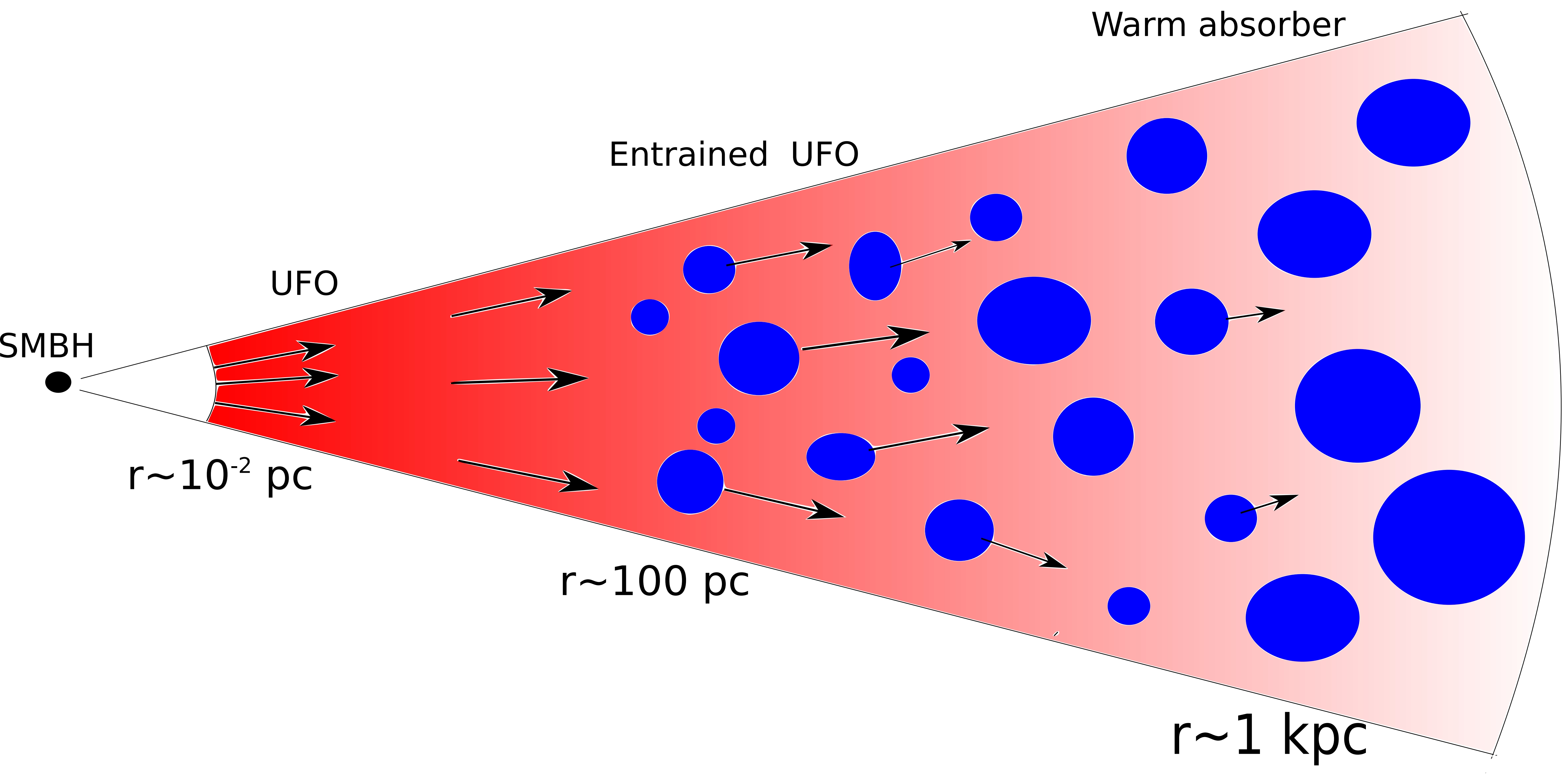
Figure 8: Diagram of the X-ray observations of PG 1114+445. A UFO is present in the inner part of the AGN surroundings, with decreasing density, scaling as $r^{-2}$. At larger distances from the SMBH, the UFO interacts with the closest clumpy ambient gas at $r\simeq 100$ pc, entraining it via Rayleigh-Taylor and Kelvin-Helmholtz instabilities. This gas is pushed at velocities comparable with that of the UFO, retaining its ionization state and column density. The farther ambient gas remains unaffected by the UFO and therefore moves at a significantly lower line-of-sight velocity. The figure is not to scale.

We summarize our findings in graphical form by presenting the multiphase absorber of PG 1114+445 in the diagram shown in Fig. 8. Together with the analysis described in this work, such a scenario is also well supported by theoretical models of AGN outflow evolution (e.g., King, 2003, 2005; Zubovas & King, 2012), which predict an inner UFO driving into the surrounding medium, sweeping-up the gas outwards. In the aftermath of the shock, four regions are consequently formed: (i) the innermost region, containing the unshocked UFO, (ii) the shocked inner wind, (iii) the shock-induced swept-up interstellar gas, and (iv) the unaffected ambient medium.
A UFO with high velocity ($v_{\text{out},3}\simeq 0.145c$), ionization parameter, and column density (e.g., Tombesi et al., 2011) is detected in three XMM-Newton observations. This absorber is located very close to the source, at $r\sim 3\times 10^{-3}\text{ pc}\simeq 60r_{\text{s}}$ (see Table 2), and can be associated with the inner wind, in agreement with detailed general-relativistic radiative magnetohydrodynamic (GR-rMHD) simulations (e.g., Sa̧dowski & Gaspari, 2017). On the contrary, given its expected low particle density (see Sect. 5), the shocked inner wind is likely to be undetectable with the present dataset, since an expected column density of $N_{\text{H}}\sim 10^{16}$ cm^-2 is below the sensitivity limit of current spectrometers.
The low values of $v$, $\log\xi$, and $N_{\text{H}}$ for the WA are compatible with usual absorbers of this kind (e.g., Blustin et al., 2005). Its low variability (see Fig. 4) suggests that the WA is not dynamically connected to the inner UFO. In fact, WAs are believed to be relics of the original optically thick gas surrounding the black hole before any AGN activity started. This gas may have been driven towards larger distances by the initial radiation pressure of the quasar, until it became optically thin (King & Pounds, 2014). Alternatively, the ambient clouds are drifting in the macro-scale turbulent velocity field (Gaspari & Sa̧dowski, 2017), with velocities of a few hundred km s^-1. Supported by the constancy over more than a decade of observations, the WA is most likely part of the ambient medium, not yet significantly affected by the UFO.
A comparison between the $v-\xi$, $v-N_{\text{H}}$ and $\xi-N_{\text{H}}$ relations for the three absorbers (see Figs. 5, 6, and 7) shows that the WA and the UFO are well around the expected values (Tombesi et al., 2013), whereas, on the other hand, the E-UFO has the typical velocity of a UFO, but ionization and column density values comparable with the WA.
We interpret these three main absorbers phases as the time evolution of outflows that were expelled at different epochs from the SMBH accretion disk and are observed as the material is continuing to travel outwards. These considerations are valid under the plausible assumption that the mass accretion rate of the SMBH, and consequently the power of the UFO, did not significantly change during a timescale of $t\sim r/v\sim 100\text{ pc}/0.145c\sim 2,000$ years, which is negligible compared to the minimum time required for the SMBH to double its mass, equal to the Salpeter time $t_{S}\sim 5\times 10^{7}$ yrs. Moreover, we note that in low-mass galaxy haloes, the AGN accretion duty cycle is almost quasi-continuous, thus allowing for the observation of multiple generations of AGN feedback events (Gaspari & Sa̧dowski, 2017). Finally, the interaction between the UFO and the clumpy ambient medium is most likely Rayleigh-Taylor and Kelvin-Helmholtz unstable (e.g., King, 2010; Zubovas & Nayakshin, 2014; Costa et al., 2014), consistently with the variability of the E-UFO and its low volume filling factor $C_{v}$.
Our detection of three concurrent outflow phases in the same source provides a remarkable corroboration of the self-regulated mechanical AGN feedback scenario (e.g., King, 2003, 2005; King & Pounds, 2014; Gaspari & Sa̧dowski, 2017). Similar conclusions, however not considering a clumpiness of the ambient medium, have been reached by Sanfrutos et al. (2018), for IRAS 17020+4544, in which all three phases have also been detected. The UFO, driven by the accreting SMBH, propagates to meso scales (parsec to kiloparsec), still with significant velocity, where the entrainment and mixing with the turbulent and clumpy ambient medium becomes substantial (E-UFO). The outflow kinetic energy is then likely deposited at macro scales in the form of thermal energy, via bubbles, shocks, and turbulent mixing (Gaspari & Sa̧dowski, 2017; Lau et al., 2017), thus re-heating the galaxy and the group gaseous halo. This self-regulated cycle may happen many times during the AGN’s lifetime, giving rise to a symbiotic relation between the SMBH growth and the evolution of the host galaxy (Gaspari et al., 2017).
The combination of multiepoch observations of nuclear winds and multiwavelength investigations of spectral features tracing multiphase parsec to kiloparsec outflows (e.g., Fiore et al., 2017) can be considered as the most promising strategy to shed light on the AGN feedback processes over a large range of distances from the central engine. In particular, UV and optical spectra of PG 1114+445 are currently being analyzed in order to link the physical properties of outflows in different spectral bands and will be the subject of upcoming articles.

Appendix A Data

Table 3: Data considered in this work for PG 1114+445.

ID	OBSID	Start date	Instrument	Exposure time (s)	Counts (0.3-10 keV)
A	74072000	1996-05-05 23:59:48	ASCA sis0+1	121230	6089*
			ASCA gis2+3	136800	6138*
0	0109080801	2002-05-14 15:27:00	EPIC-pn	32500	23462
			MOS1+2	80380	17700
1	0651330101	2010-05-19 09:48:59	EPIC-pn	20550	7166
			MOS1+2	57270	6418
2	0651330201	2010-05-21 09:41:13	EPIC-pn	9824	3924
			MOS1+2	27400	3213
3	0651330301	2010-05-23 10:06:23	EPIC-pn	5271	1669
			MOS1+2	18357	1792
4	0651330401	2010-06-10 07:28:14	EPIC-pn	10740	5341
			MOS1+2	32750	5214
5	0651330501	2010-06-14 07:56:46	EPIC-pn	6613	2956
			MOS1+2	16804	2314
6	0651330601	2010-11-08 23:22:49	EPIC-pn	18500	17359
			MOS1+2	46400	12704
7	0651330701	2010-11-16 22:50:52	EPIC-pn	16240	9732
			MOS1+2	46510	9046
8	0651330801	2010-11-18 22:42:54	EPIC-pn	20350	9707
			MOS1+2	57020	8490
9	0651330901	2010-11-20 22:35:32	EPIC-pn	21350	12244
			MOS1+2	52210	9724
10	0651331001	2010-11-26 23:40:17	EPIC-pn	17660	8704
			MOS1+2	46040	7173
11	0651331101	2010-12-12 22:31:31	EPIC-pn	13710	7439
			MOS1+2	26650	4562

Appendix B Tables of best-fit results

Table 4: Parameters of Abs. 1.

ID	$N_{\text{H},1}/10^{21}$ cm-2	$\log(\xi_{1}/$erg cm s-1)	$\Delta\chi^{2}$
A	$7.5^{*}$	$0.35^{*}$	$275$
0	$7.7_{-0.4}^{+0.3}$	$0.34_{-0.01}^{+0.01}$	$1990$
1+2+3	$7.5^{*}$	$0.35^{*}$	$1377$
4+5	$6.9_{-3.1}^{+0.7}$	$\leq 0.32$	$1117$
6	$7.5_{-0.5}^{+0.6}$	$0.35_{-0.02}^{+0.04}$	$1852$
7	$7.9_{-0.3}^{+0.5}$	$0.33_{-0.01}^{+0.01}$	$1073$
8+9	$7.4_{-0.5}^{+0.5}$	$0.34_{-0.01}^{+0.02}$	$2182$
10	$7.6_{-1.0}^{+0.6}$	$0.37_{-0.03}^{+0.06}$	$880$
11	$7.5^{*}$	$0.35^{*}$	$648$

Table 5: Parameters of Abs. 2.

ID	$N_{\text{H},2}/10^{21}$ cm-2	$\log(\xi_{2}/$erg cm s-1)	$z_{\text{o},2}/10^{-2}$	$v_{2}/c$	$\Delta\chi^{2}$	$P_{\text{null}}$
A	$7.8_{-1.4}^{+0.6}$	$0.34_{-0.06}^{+0.63}$	$+3.3_{-2.4}^{+3.9}$	$0.102_{-0.037}^{+0.023}$	$46$	$10^{-12}$
0	$1.8_{-0.1}^{+0.2}$	$0.65_{-0.04}^{+0.10}$	$+1.7_{-1.3}^{+1.4}$	$0.117_{-0.012}^{+0.013}$	$68.4$	$10^{-11}$
1+2+3	$3.7_{-0.1}^{+0.1}$	$0.26_{-0.03}^{+0.05}$	$-3.9_{-1.8}^{+1.2}$	$0.172_{-0.018}^{+0.012}$	$18.1$	$10^{-3}$
4+5	$7.7_{-0.2}^{+0.3}$	$0.38_{-0.01}^{+0.01}$	$+6.4_{-1.4}^{+1.5}$	$0.073_{-0.013}^{+0.014}$	$20.4$	$3\times 10^{-4}$
6	$2.7_{-0.2}^{+0.2}$	$0.06_{-0.02}^{+0.02}$	$-2.1_{-1.4}^{+1.2}$	$0.155_{-0.014}^{+0.012}$	$61$	$3\times 10^{-11}$
7	$6.7_{-1.0}^{+0.9}$	$1.39_{-0.10}^{+0.07}$	$+6.4_{-1.6}^{+1.3}$	$0.073_{-0.015}^{+0.012}$	$26.0$	$6\times 10^{-6}$
8+9	$3.0_{-0.1}^{+0.2}$	$0.63_{-0.03}^{+0.06}$	$+1.1_{-0.8}^{+1.0}$	$0.123_{-0.008}^{+0.010}$	$73.4$	$4\times 10^{-15}$
10	$3.0_{-0.2}^{+0.2}$	$0.35_{-0.05}^{+0.04}$	$+1.4_{-1.6}^{+1.2}$	$0.132_{-0.016}^{+0.012}$	$32.1$	$10^{-6}$
11	$5.4_{-0.6}^{+0.7}$	$1.22_{-0.08}^{+0.07}$	$+3.6_{-2.0}^{+1.0}$	$0.100_{-0.019}^{+0.009}$	$78$	$3\times 10^{-12}$

Table 6: Parameters of Abs. 3.

ID	$N_{\text{H},3}/10^{21}$ cm-2	$\log(\xi_{3}/$erg cm s-1)	$z_{\text{o},3}/10^{-2}$	$v_{3}/c$	$\Delta\chi^{2}_{\text{2abs}}$	$P_{\text{null,2abs}}$	$\Delta\chi^{2}_{\text{1abs}}$	$P_{\text{null,1abs}}$
A	$\geq 440$	$3.83_{-0.21}^{+0.21}$	$+0.2_{-0.5}^{+0.5}$	$0.132_{-0.005}^{+0.005}$	/	/	/	/
1+2+3	$143_{-69}^{+606}$	$3.85_{-0.14}^{+0.47}$	$+5.9_{-0.9}^{+0.5}$	$0.078_{-0.008}^{+0.005}$	$20.0$	$4\times 10^{-4}$	$21.1$	$3\times 10^{-4}$
6	$\geq 295$	$4.43_{-0.34}^{+0.22}$	$-1.2_{-0.4}^{+0.5}$	$0.145_{-0.004}^{+0.005}$	$11.8$	$0.01$	$13.5$	$0.01$
8+9	$75_{-36}^{+125}$	$3.77_{-0.13}^{+0.23}$	$-4.7_{-0.7}^{+0.5}$	$0.173_{-0.007}^{+0.005}$	$12.0$	$7\times 10^{-3}$	$12.4$	$0.01$

Table 7: Blackbody temperatures and photon indices of each observation.

ID	$kT/10^{-2}$ keV	$\Gamma$	$\chi^{2}/\text{dof}$	Fitted absorbers
A	$6.4_{-1.1}^{+1.2}$	$1.84_{-0.08}^{+0.05}$	$538.0/427$	3
0	$6.0_{-0.3}^{+0.2}$	$1.68_{-0.02}^{+0.04}$	$525.7/445$	2
1+2+3	$7.0_{-0.2}^{+0.2}$	$1.44_{-0.02}^{+0.04}$	$500.3/464$	3
4+5	$6.1_{-0.7}^{+0.6}$	$1.68_{-0.06}^{+0.05}$	$295.4/296$	2
6	$5.5_{-0.3}^{+0.3}$	$1.62_{-0.03}^{+0.03}$	$389.2/372$	3
7	$5.5_{-0.3}^{+0.6}$	$1.63_{-0.07}^{+0.04}$	$264.0/288$	2
8+9	$6.3_{-0.4}^{+0.3}$	$1.53_{-0.02}^{+0.02}$	$649.4/663$	3
10	$6.7_{-0.6}^{+0.9}$	$1.58_{-0.06}^{+0.05}$	$246.1/246$	2
11	$6.7_{-0.3}^{+0.2}$	$1.59_{-0.06}^{+0.09}$	$232.0/195$	2

Appendix C Comparison between XMM-Newton cameras

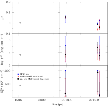
Figure 10: Best-fit values of the pn camera (blue squares), the MOS cameras combined (red triangles), and pn and MOS data together (black circles) of the three parameters of Abs. 3. The star is the ASCA value. The parameters are in agreement within their errors at $90\%$ confidence level. The horizontal black line represents the cosmological redshift of the source, $z_{o}=0.144$.

Appendix D Spectra

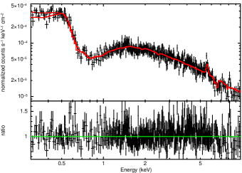
Figure 12: Spectrum and ratio of Obs. 1+2+3. The red line is the best fit.

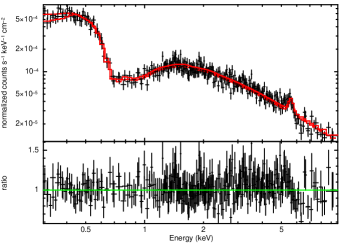
Figure 13: Spectrum and ratio of Obs. 4+5. The red line is the best fit.

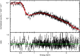
Figure 14: Spectrum and ratio of Obs. 6. The red line is the best fit.

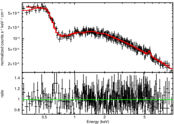
Figure 15: Spectrum and ratio of Obs. 7. The red line is the best fit.

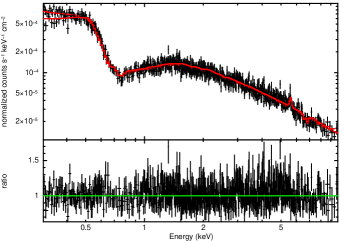
Figure 16: Spectrum and ratio of Obs. 8+9. The red line is the best fit.

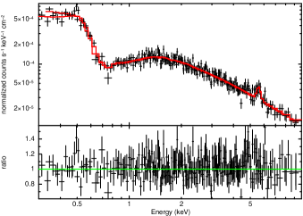
Figure 17: Spectrum and ratio of Obs. 10. The red line is the best fit.

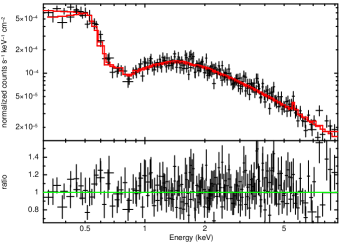
Figure 18: Spectrum and ratio of Obs. 11. The red line is the best fit.