Kardar-Parisi-Zhang Scaling for an Integrable Lattice Landau-Lifshitz Spin Chain

Abstract

Recent studies report on anomalous spin transport for the integrable Heisenberg spin chain at its isotropic point. Anomalous scaling is also observed in the time-evolution of non-equilibrium initial conditions, the decay of current-current correlations, and non-equilibrium steady state averages. These studies indicate a space-time scaling with $x\sim t^{2/3}$ behavior at the isotropic point, in sharp contrast to the ballistic form $x\sim t$ generically expected for integrable systems. In our contribution we study the scaling behavior for the integrable lattice Landau-Lifshitz spin chain. We report on equilibrium spatio-temporal correlations and dynamics with step initial conditions. Remarkably, for the case with zero mean magnetization, we find strong evidence that the scaling function is identical to the one obtained from the stationary stochastic Burgers equation, alias Kardar-Parisi-Zhang equation. In addition, we present results for the easy-plane and easy-axis regimes for which, respectively, ballistic and diffusive spin transport is observed, whereas the energy remains ballistic over the entire parameter regime.

I Introduction

Classical Hamiltonian systems are usually classified as non-integrable and integrable, depending on whether they possess either a small or a macroscopically large number of conserved fields. More precisely, a Hamiltonian system with $N$ degrees of freedom is called integrable if one can find $N$ independent constants of motion – otherwise, it is referred to as non-integrable. In general, one would expect integrable and non-integrable systems to have drastically different transport properties. Let us consider the example of a translation invariant one-dimensional mechanical system with $Q=\sum_{j=1}^{N}Q_{j}$ a conserved field satisfying a local conservation law of the form $\partial Q_{j}/\partial t=J_{j}-J_{j+1}$, where $J_{j}$ is the corresponding local current. The corresponding dynamical equilibrium correlation function is defined by

$$C(j,t)=\langle Q_{j}(t)Q_{0}(0)\rangle^{\mathrm{c}}_{\rm eq},$$ (1)

where the average is over initial conditions chosen from the Gibbs equilibrium distribution and the superscript denotes the connected part of the correlator, defined as $\langle Q_{j}(t)Q_{0}(0)\rangle^{\mathrm{c}}_{\rm eq}:=\langle(Q_{j}(t)-\langle Q_{0}\rangle_{\rm{eq}})(Q_{0}(0)-\langle Q_{0}\rangle_{\rm{eq}})\rangle_{\rm{eq}}$. Since $Q$ is conserved, one expects a scaling form as

$$C(j,t)=\chi(\Gamma t)^{-\alpha}f\big{(}(\Gamma t)^{-\alpha}(j-ct)\big{)}.$$ (2)

$\alpha>0$ is the scaling exponent, $c$ a potential systematic shift (the “sound” velocity), $\Gamma$ a model dependent parameter, and $f$ the scaling function normalized with total sum equal to $1$. Our particular form ensures that $\sum_{j}C(j,t)=\chi$ independent of $t$, and $\chi$ is the static susceptibility. For integrable systems most commonly $\alpha=1$ and $c=0$, which is the ballistic behavior. The scaling function depends on $Q$. On the other hand, in non-integrable systems one often observes $\alpha=\tfrac{1}{2}$ with a Gaussian scaling function. But also anomalous scaling with $\alpha=\tfrac{2}{3}$ has been discovered MendlSpohnPRL13 ; mendl14 ; SGDasPRE2014 ; Kulkarni2013 ; Kulkarni2015 ; spohn2014 ; SGDasArXiv2014 ; das2019 . Such differences between integrable and non-integrable systems are also observed in other transport simulations, for instance in the evolution of non-equilibrium initial conditions and in properties of boundary driven non-equilibrium steady states (NESS). Through generalized hydrodynamics much progress has been accomplished in the understanding of transport in integrable systems spohn2018 ; doyon2018 ; PhysRevLett.121.230602 ; PhysRevX.6.041065 ; moore2017 ; PhysRevLett.117.207201 .

A surprising exception to the generic behavior has been discovered for spin transport in the integrable XXZ Heisenberg spin chain. The quantum $XXZ$ spin $\tfrac{1}{2}$ chain is Bethe ansatz solvable for an arbitrary choice of the anisotropy parameter $\Delta$. The spectrum is gapless for $|\Delta|\leq 1$ and gapped otherwise. A number of studies find that, for zero $z$-magnetization, spin transport in this system is diffusive for $\Delta>1$, ballistic for $\Delta<1$ and anomalous at $\Delta=1$. First indications of this behavior came from the Drude weight for spin transport zotos1997 ; zotos1999 ; affleck2011 . Subsequent evidence was obtained in NESS studies at infinite temperatures prosen2009 ; znidaric2011 , in the form of equilibrium correlation functions Gemmer2009 , and in the evolution of quenched initial conditions moore2014 . There has been some understanding of the un-expected diffusive and anomalous regimes of spin transport using the GHD framework vasseur2018 ; PhysRevLett.121.230602 .

The goal of our contribution is to find out whether a similar pattern persists in corresponding classical models. One natural choice would be the classical Heisenberg model on the one-dimensional continuum, also known as the Landau-Lifshitz model, which is integrable and has the same rotational symmetries as the XXZ chain c1 ; c2 ; c3 ; c4 . However numerical discretizations schemes might spoil integrability. Also the equilibrium states live on non-smooth spin configurations. For these reasons it is better to keep the underlying lattice, leading to the lattice Landau-Lifshitz (LLL) model, which in fact is non-integrable. Recent work das2019 has explored spin and energy correlations. They turn out to be diffusive at high temperatures, while anomalous features emerge at low temperatures. Fortunately one can adjust the coupling function between nearest neighbors on the lattice in such a way that the model is integrable and still has the usual rotational symmetries sklyanin1982 ; sklyanin1988 ; faddeev2007 . We will refer to this model as the integrable lattice Landau-Lifshitz (ILLL) system. The ILLL model has a parameter $\rho$, which plays the role of the anisotropy parameter $\Delta$ in the Heisenberg model, such that $\rho>0$ corresponds to easy-plane and $\rho<0$ corresponds to easy-axis, while $\rho\rightarrow 0$ is the isotropic case. At the isotropic point all three components of the total magnetization are conserved. For zero average magnetization the corresponding current correlations were studied in prosen2013 . Quite remarkably, the current correlation shows an exponential decay for easy-axis ($\rho<0$) and hence a vanishing Drude weight and diffusive transport. Saturation to a non-zero value is observed for easy-plane ($\rho>0$), implying a finite Drude weight and ballistic transport. For the isotropic model an anomalous decay of the form $\sim t^{-\alpha}$ with $\alpha\approx 0.65$ is found. In our contribution we investigate the scaling properties of equilibrium space-time correlations, for both spin and energy transport, again for zero average magnetization. We confirm the scaling exponents from previous studies for spin transport in different parameter regimes. In addition, we determine the scaling functions: Gaussian for the case of diffusive transport in the easy-axis regime, while at the isotropic point, remarkably, we have a convincing fit to the Kardar-Parisi-Zhang (KPZ) scaling form $f_{\mathrm{KPZ}}$ [described later in Equation. (13)] . The energy transport remains ballistic in all regimes.

Returning to the quantum XXZ chain, in prosen2017 ; PhysRevLett.117.207201 the time evolution of the magnetization profile with a tiny initial step is studied. As expected from linear response, it is observed that for $\Delta>1$ the magnetization profile has diffusive scaling $\alpha=\tfrac{1}{2}$, while, for $\Delta=1$, the respective scaling function is anomalous with $\alpha=\tfrac{2}{3}$. In more recent work prosen2019 , it was found that the scaling function is related to the stationary KPZ equation. Such dynamical properties live on the ballistic hydrodynamic scale and are implicitly based on the assumption of local equilibrium. A similar reasoning can be applied to classical systems and generically one expects to have comparable dynamical properties. Our study of the ILLL allows us to test more sharply whether such a conjecture holds. Indeed, we observe a clear KPZ scaling in the correlation functions. However, when investigating whether the KPZ scaling also holds for the evolution of the step-profile our data are too noisy for arriving at a definite conclusion. In a recent complementary study gamayun2019 ; misguich2019 , the classical-quantum correspondence has been analyzed in the context of the continuum Landau-Lifshitz model, which is integrable, and the quantum XXZ model at zero temperature.

Our paper is organized as follows. In Sec. II, we provide the details of the model, discuss the quantities of interest, and give a brief analysis using linear response theory. We also describe the numerical methods used. Sec. III focuses on analyzing the equilibrium time correlations for all the three cases of the classical ILLL chain – isotropic, easy-plane, and easy-axis regimes. In Sec. IV, we study the evolution of an initial step magnetization profile and its scaling. We summarize our findings in Sec. V along with an outlook.

II The classical chain

The classical ILLL sklyanin1982 ; sklyanin1988 ; faddeev2007 spin chain for $N$ spins, $\vec{S}_{j},j=1,...,N$, $|\vec{S}_{j}|=1$, is defined by the following Hamiltonian

$$H=\sum_{j=1}^{N}h(\vec{S}_{j},\vec{S}_{j+1}),$$ (3)

where the nearest neighbor interactions are given by

$$h(\vec{S},\vec{S^{\prime}})=-\log\big{|}\cos(\gamma S^{(z)})\cos(\gamma S^{\prime(z)})$$

$$\hskip 10.0pt+(\cot(\gamma))^{2}\sin(\gamma S^{(z)})\sin(\gamma S^{\prime(z)})$$

$$\hskip 10.0pt+(\sin(\gamma))^{-2}G(S^{(z)})G(S^{\prime(z)})(S^{(x)}S^{\prime(x)}+S^{(y)}S^{\prime(y)})\big{|},$$

$$G(x)=\big{(}1-x^{2}\big{)}^{-\tfrac{1}{2}}\big{(}\cos(2\gamma x)-\cos(2\gamma)\big{)}^{\frac{1}{2}}.$$ (4)

$\gamma$ is the model parameter which can be either real or purely imaginary. Without loss of generality, we introduce the new parameter $\rho=\gamma^{2}$, $\rho\in\mathbb{R}$. The boundary conditions will be taken to be either periodic or open, depending on the particular physical situation studied. Easy-plane corresponds to $\rho>0$, easy-axis to $\rho<0$, while in the limit $\rho\to 0$ one obtains the isotropic interaction,

$$h\left(\vec{S},\vec{S^{\prime}}\right)=-\log\left(1+\vec{S}\cdot\vec{S^{\prime}}\right).$$ (5)

Note that the $``-"$ sign in front of $h$ corresponds to the ferromagnetic interaction, whereas the positive sign will correspond to an anti-ferromagnetic interaction. In the present work we focus on the ferromagnetic Hamiltonian. For the anti-ferromagnetic case, the potential is not bounded from below and hence there would be equilibration problems at low temperatures. To see this, we note that for the general case with $h(\vec{S},\vec{S^{\prime}})=-J\log\big{(}1+\vec{S}\cdot\vec{S^{\prime}}\big{)}$, with $J>0$ ($J<0$) corresponding to ferromagnetic (antiferromagnetic) interactions, the equilibrium state is given by,

$$\prod_{j}\big{(}1+\vec{S}_{j}\cdot\vec{S}_{j+1}\big{)}^{\beta J}.$$ (6)

For $J<0$ this Boltzmann weight becomes unbounded as two neighboring spins point oppositely and can no longer be normalized once $\beta J\leq-1$. Close to that value typically the chain will have long anti-ferromagnetic domains, which slow down the evolution. A trace of this feature is still present at $\beta=0$. Thus we find for $\beta=0$ and $J=1$ that after $10^{6}$ averages the data are still too noisy to pin down the tail behavior. More precise numerical data are achieved for $\beta=1$, and we use this value for all the simulations presented in this paper.

The dynamics of spins is governed by Hamilton’s equations of motion,

$$\frac{d}{dt}\vec{S}_{j}=\{\vec{S}_{j},H\}=\vec{S}_{j}\times\vec{B}_{j},\quad\vec{B}_{j}=-\nabla_{\vec{S}_{j}}H.$$ (7)

We study transport in this model, through both equilibrium and nonequilibrium properties.
(i) In the equilibrium simulations we use periodic boundary conditions and compute spin and energy space-time correlators defined by

$$C_{\mathrm{ss}}(j,t) =\langle S_{j}^{(z)}(t)S_{0}^{(z)}(0)\rangle^{\mathrm{c}}_{\mathrm{eq}},$$

$$C_{\mathrm{ee}}(j,t) =\langle e_{j}(t)e_{0}(t)\rangle^{\mathrm{c}}_{\mathrm{eq}}$$ (8)

where $e_{j}=h(\vec{S}_{j},\vec{S}_{j+1})$ and the truncated average $\langle\dots\rangle^{\mathrm{c}}_{\mathrm{eq}}$ is taken with respect to the equilibrium distribution $e^{-\beta H}/Z$.
(ii) In the nonequilibrium simulations, we consider an open XXX chain initially prepared with a uniform temperature and a step in the magnetization. More precisely, the initial state is $Z^{-1}\exp\big{[}-\beta\big{(}H-\sum_{j}h_{j}^{(z)}S_{j}^{(z)}\big{)}\big{]}$, where $h_{j}^{(z)}=-h_{0}$ for $j\leq 0$ and $h_{j}^{(z)}=h_{0}$ for $j>0$. Of interest is the average magnetization $s(j,t)=\langle S^{(z)}_{j}(t)\rangle_{h_{0}}$ at time $t$, where the dynamics is according to $H$ and the index recalls the dependence of the initial state on $h_{0}$. If the step is small, this average can be expanded in $h_{0}$. The zeroth order vanishes and, using that $C_{\mathrm{ss}}(j,t)=C_{\mathrm{ss}}(-j,t)$, to first order one arrives at

$$s(j,t) =\beta\sum_{i}h^{(z)}_{i}C_{\mathrm{ss}}(j-i,t)$$ (9)

$$=\beta h_{0}\bigg{(}C(0,t)+2\sum_{i=1}^{j}C_{\mathrm{ss}}(i,t)\bigg{)}$$

for $j\geq 1$ with $s(-j+1,t)=-s(j,t)$. As a consequence, if $C_{\mathrm{ss}}(j,t)$ scales as in (2) with $c=0$, then $s(j,t)$ inherits the corresponding scaling. In the continuum form one arrives at

$$s(x,t)=2\beta h_{0}\chi\int_{0}^{x/(\Gamma t)^{\alpha}}dx^{\prime}f(x^{\prime})$$ (10)

for $x\geq 0$. The derivative of the scaling function of $s$ yields the scaling function for $C$. For example, if $C_{\mathrm{ss}}$ has Gaussian scaling, then $s(x,t)$ would scale with the error function. Note that the scaling exponent remains unchanged.

KPZ equation and scaling functions. KPZ equation describes the surface growth under a random ballistic deposition. The height function $h(x,t)$ is governed by the Langevin equation,

$$\partial_{t}h=\tfrac{1}{2}\lambda(\partial_{x}h)^{2}+\nu\partial_{x}^{2}h+\sqrt{D}\eta,$$ (11)

where $\eta$ is normalized space-time white noise. The slope $u(x,t)=\partial_{x}h(x,t)$ is governed by the stochastic Burgers equation

$$\partial_{t}u+\partial_{x}\big{(}-\tfrac{1}{2}\lambda u^{2}-\nu\partial_{x}u-\sqrt{D}\eta\big{)}=0.$$ (12)

In the stationary state the mean of $u$ can be chosen to vanish and $x\mapsto u(x,0)$ is spatial white noise of strength $\chi=D/2\nu$. As shown in prahofer2004exact the two-point function of the stationary stochastic Burgers equation is given by

$$\langle u(0,0)u(x,t)\rangle\sim\chi(\Gamma t)^{-2/3}f_{\mathrm{KPZ}}\left((\Gamma t)^{-2/3}x\right).$$ (13)

$\Gamma$ determines the non-universal time scale, which in the case of the Burgers equation turns out to be $\Gamma=\sqrt{2}\lambda$. The scaling function $f_{\mathrm{KPZ}}(x)$ is positive, symmetric relative to the origin, and normalized to $1$. It looks like a Gaussian in bulk but has tails which decay as $\exp(-0.295|x|^{3})$, hence faster than a Gaussian.
Simulation details. We integrate the evolution equation (7) using the adaptive Runge-Kutta method flannery1992numerical . In some some regions in configuration space, the logarithmic interaction potential is very steep, and because of this the fixed step-size Runge-Kutta method turned out to be insufficient, especially at large times. One challenge is to keep the energy and the lengths of individual spins conserved during the numerical integration. Both these quantities dissipate quite a bit with time due to the accumulation of numerical errors. We give the input tolerance in the adaptive algorithm such that at the final time total energy remains conserved up to four decimal places and individual lengths of spins up to five decimal places. Total magnetization remains conserved well, up to 13 decimal places.

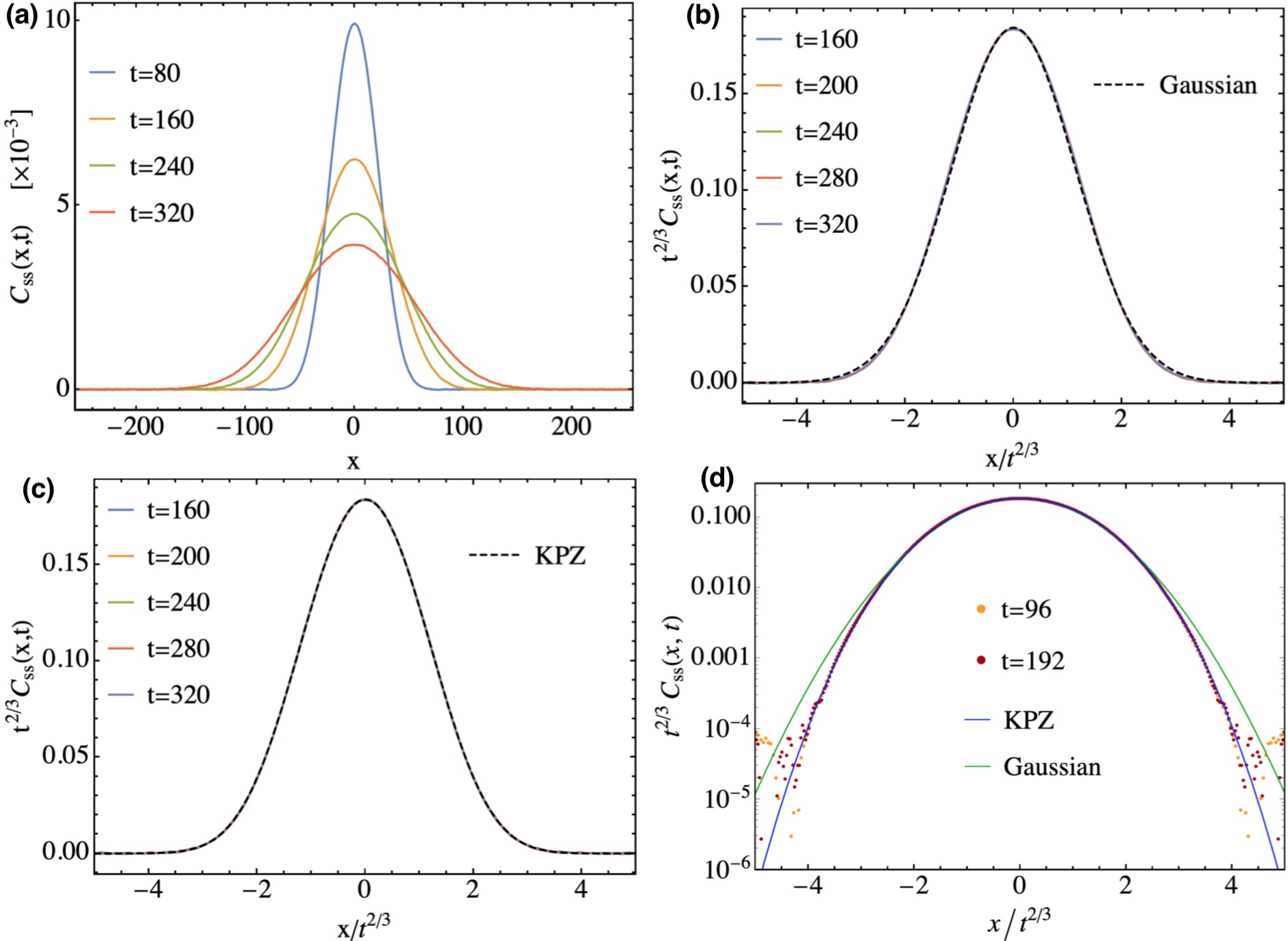
Figure 1: (Isotropic regime) (a) Plot of the spin-spin correlation $C_{\mathrm{ss}}(x,t)$. And the same after a $t^{2/3}$ scaling with a fit to (b) Gaussian and (c) the KPZ scaling functions. In (d) we show the two fits compared to the data in logarithmic $y-$scale. This plot reveals that the KPZ scaling function offers a much better fit to the data. Parameter values: system size = $2048$, averaging over $\sim 10^{6}$ initial conditions and inverse temperature $\beta=1$.

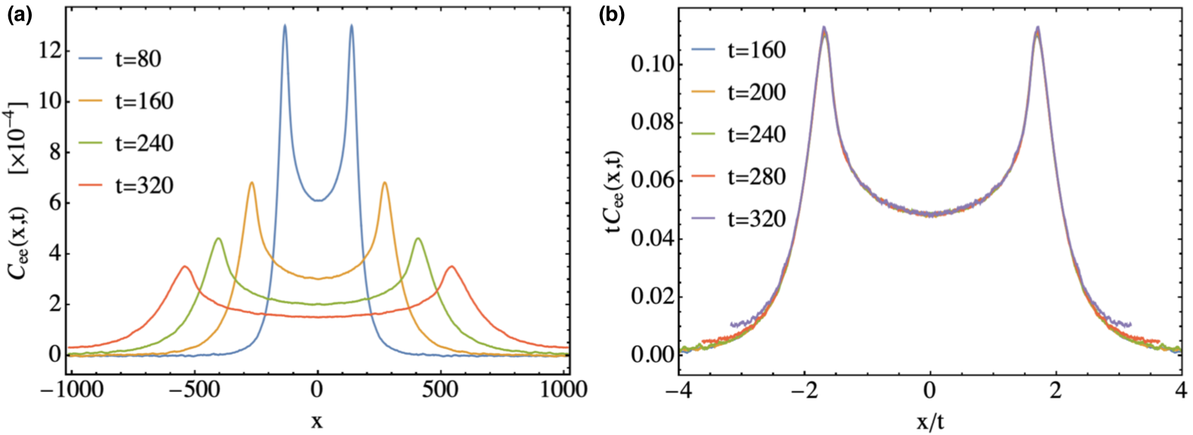
Figure 2: (Isotropic regime) Plot of the energy-energy correlation $C_{ee}(x,t)$ and the ballistic scaling of it. Parameter values: system size = 2048, final time = 320, averaging over $\sim 10^{6}$ initial conditions and inverse temperature $\beta$ = 1.

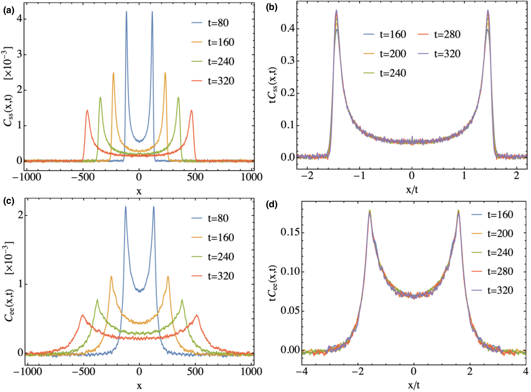
Figure 3: (Easy plane regime) Plot of the spin-spin correlation $C_{\mathrm{ss}}(x,t)$ and energy-energy correlation $C_{ee}(x,t)$ in easy-plane regime and corresponding ballistic scalings. Parameter values: system size =$2048$, averaging over $\sim 4\times 10^{4}$ initial conditions and inverse temperature $\beta=1$.

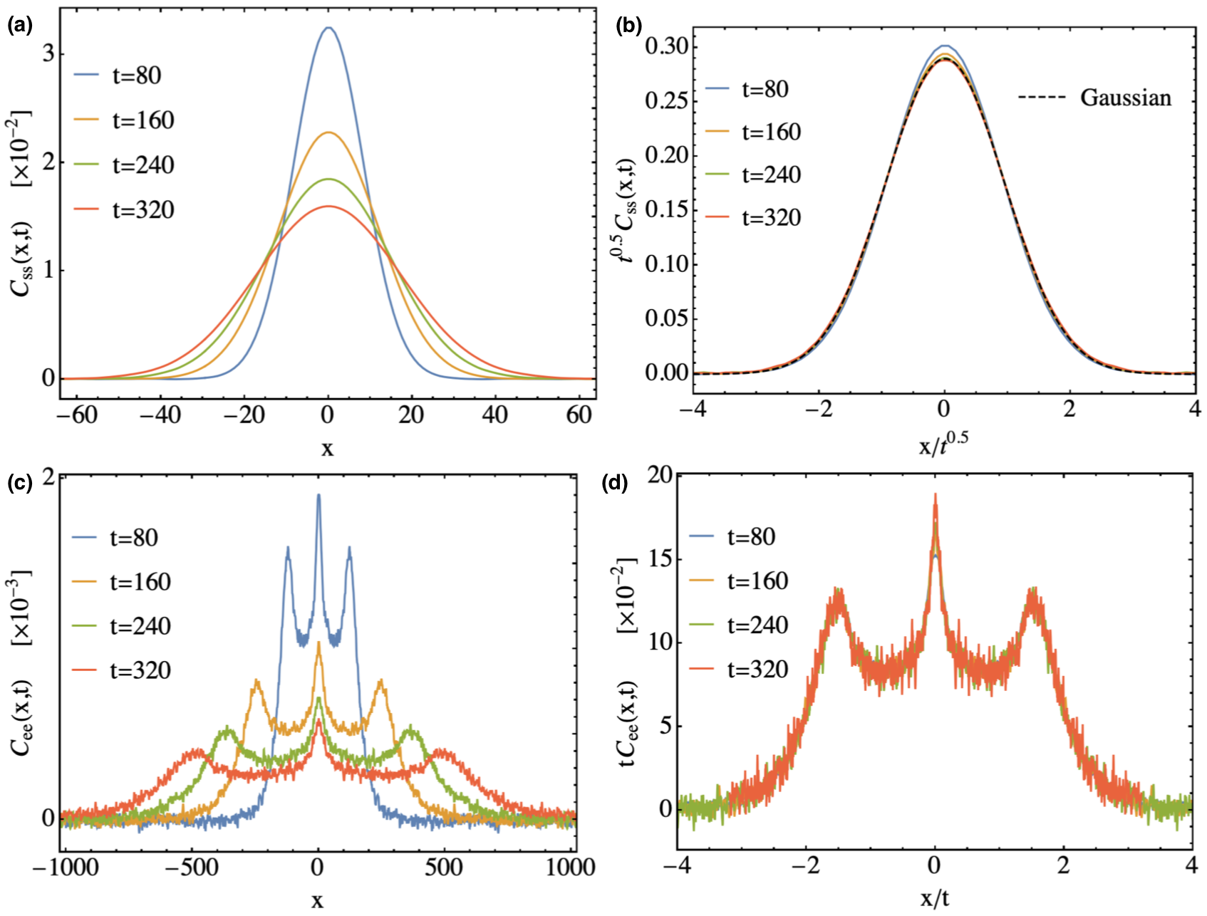
Figure 4: (Easy axis regime) Spin-spin correlation $C_{\mathrm{ss}}(x,t)$ and energy-energy correlation $C_{ee}(x,t)$ in easy-axis regime. In (b) we show the diffusive scaling of spin correlations while in (d) we see the ballistic scaling of energy correlations. Parameter values: system size = $2048$, averaging over $\sim 4\times 10^{4}$ initial conditions and inverse temperature $\beta=1$.

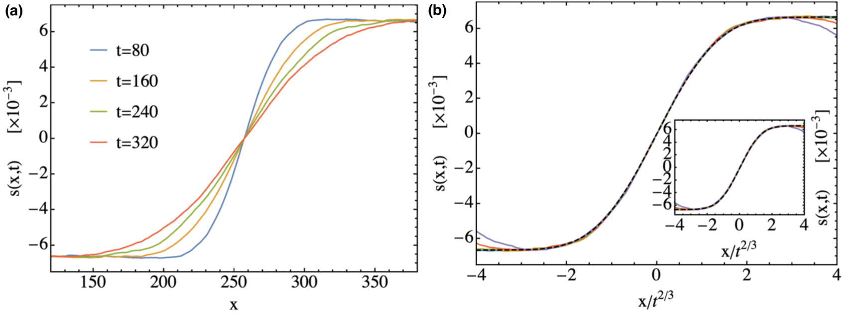
Figure 5: (Isotropic regime) (a) Magnetization profile at different times starting from a step initial condition. (b) Collapse of the data under a $t^{2/3}$ scaling. The dashed line corresponds to the integrated KPZ scaling function (10). Inset shows the fit with integrated Gaussian, namely the Error function. Although the $2/3$ scaling is prominent, we cannot distinguish the (integrated) Gaussian and KPZ here. Parameter values: System size = $512$, inverse temperature $\beta=1$ and averaging over $\sim 8\times 10^{5}$ initial conditions.

We use Metropolis Monte Carlo sampling to generate the canonical ensemble. Starting from an ordered initial configuration, we allow $5000$ Monte Carlo swipes to make sure that the system has reached thermal equilibrium at the desired temperature. Once equilibrium has reached, we drop $500$ swipes every time we generate a new thermal configuration to use as the initial condition for the time evolution. Thereby one ensures that the initial conditions used in the time evolution are sufficiently uncorrelated among themselves. All averages are taken over these initial conditions. The step initial profile is generated by equilibrating the system using a step magnetic field of the appropriate size at given temperature. In our study we chose the value of $\beta=1$. At higher temperatures, the average energy per site increases and the spins access the steeper parts of the inverted log potential [see (II)] and as a result the simulation using the adaptive step size algorithm becomes very slow [see discussion around Eq. (6)]. For the choice $\beta=1$, the simulation efficiency is reasonable and it is expected that our main results should be valid at other temperatures.

III Simulation results for equilibrium dynamical correlations

III.1 Isotropic regime

This corresponds to the choice $\rho\rightarrow 0$ in (II), which leads to the simpler form of the Hamiltonian (5). In this regime, spins have no directional bias and lie uniformly on the unit sphere. At infinite temperature these directions don’t have any correlation but at finite and low temperatures the correlation grows. In Fig. 1(a) we plot the spin-spin correlation function $C_{\mathrm{ss}}(x,t)$ for $\beta=1$. We see a very good $x\sim t^{2/3}$ scaling of the data. In Fig. 1(b) we compare the scaled data with a Gaussian distribution, while in Fig. 1(c) we compare the same data with the KPZ distribution. We first compute the sum $\sum_{j}C_{\mathrm{ss}}(j,t)$, which is independent of time and gives an estimate of the area under the fit curve. This is essentially the value of $\chi$ in (2). Then we find the best fit parameter $\Gamma$ using the NonlinearModelFit function of Mathematica. In particular, we found that $\chi=0.526698$ and $\Gamma=1.93609$ for $f_{\mathrm{KPZ}}$ and $1.21582$ for $f_{\mathrm{Gaussian}}$. Although the distinction is not so significant on this scale, we see that a much better fit is obtained with the KPZ distribution. The distinction becomes very prominent in the log plot shown in Fig. 1(d). This is because the KPZ scaling function differs from a Gaussian only in the tails. Although spin transport is superdiffusive in this regime of the Hamiltonian, energy transport is ballistic. Energy correlations are plotted in Fig. 2 which show a clear ballistic scaling.

Note that, in many cases, the diffusive or superdiffusive modes come coupled with the ballistic modes and to see them one needs to subtract the ballistic contributions, which is a difficult task in general doyon2018 . In our case it turns out that for spin transport at the isotropic point the ballistic contribution does not exist and we directly see the superdiffusive mode.

III.2 Easy-plane regime

This corresponds to the choice $\rho>0$ in Eq. (II). Spins tend to lie near the $x-y$ plane at finite temperatures. We use the value $\rho=1$. As shown in Fig. (3), both spin and energy show ballistic scaling in this regime. We however observe that spin transport is slower than the energy transport. In other words, in Fig. 3 the line shapes for spin and energy transport are distinctly different.

III.3 Easy-axis regime

This corresponds to the choice $\rho<0$ in Eq. (II), i.e. $\gamma$ becomes purely imaginary and the trigonometric functions become hyperbolic functions in the Hamiltonian. For our purpose, we use the value $\rho=-1$. In this regime, spins have the tendency to lie near the $z$-axis at finite temperatures. As shown in Fig. 4, we now observe that spin correlations spread diffusively while energy correlations spread ballistically. In this particular regime we have diffusive transport of spin. In Table. 1, we summarize the transport properties in the ILLL chain.

IV Magnetization profile for step initial condition

We consider now a chain of $N=512$ spins and prepare it at the inverse temperature $\beta=1$ using a step magnetic field as described in Sec. II with $h_{0}=0.01$. We average over $~{}8\times 10^{5}$ such initial conditions. The resulting step height in the magnetization is $\pm 0.00665$. These step initial conditions are evolved according to the isotropic Hamiltonian (5) and we monitor the average magnetization profile $s(x,t)$ at later times. Magnetization profiles at different times are shown in Fig. 5(a), while Fig. 5(b) shows the $2/3$ scaling of $s(x,t)$. This is expected from (10) and our previous finding of $2/3$ scaling of $C_{SS}(x,t)$ in the isotropic regime. Although $s(x,t)$ correctly reproduces the scaling exponent, the data is noisy and not accurate enough for us to rule out a fit to an error function (integral of a Gaussian). In Fig. 5(b) we show the fit with integral of $f_{\mathrm{KPZ}}$ and, in the inset, we show the fit with the error function. Much more averaging over the initial conditions is required to arrive at smoother data shown here. Here we are essentially dealing with (10). This equation is supposed to be exact in the linear response limit $h_{0}\rightarrow 0$, and so one should recover the same values of $\Gamma$’s and $\chi$ obtained from $C_{\mathrm{ss}}$ data by analyzing the step profile. However, in our simulations we have kept $h_{0}=0.01$ and as a result we observe slight deviations in the $\Gamma$ and $\chi$ values. Here we see $\chi=0.665$ and $\Gamma=1.74603$ for both KPZ and Gaussian functions.

Table 1: Summary of transport properties in the ILLL model for zero $z$-magnetization

Regime	Spin transport	Energy transport
Easy plane $(\rho>0)$	Ballistic	Ballistic
Isotropic $(\rho\rightarrow 0)$	Super-diffusive scaling exponent: 2/3 scaling function: KPZ	Ballistic
Easy axis $(\rho<0)$	Diffusive scaling function: Gaussian	Ballistic

Note: Diffusive transport implies scaling exponent = 1/2 and ballistic transport implies scaling exponent = 1.

V Conclusions

From the study of several integrable many-body systems, there seems to be a consensus that their large scale behavior has many common features. In particular, since based on hydrodynamic type arguments, quantum models should not differ from their classical version. We presented the numerical study of the classical integrable ILLL spin chain and compared with previous studies of the quantum XXZ Heisenberg model. Our findings are summarized in Table 1 and support the view that on hydrodynamic scales classical and quantum cannot be distinguished. At the isotropic point with zero average magnetization, we find that the quantities involving spin show superdiffusive behavior with scaling exponent $2/3$ and the scaling function is KPZ. In the easy-plane regime, we find that the spin transport is ballistic, while in the easy-axis regime it is diffusive. The energy correlations are shown to exhibit ballistic scaling in all parameter regimes. To probe the KPZ behavior further we also studied the evolution of an initial magnetization step. Again, we find the $t^{2/3}$ scaling but, from these data, we are not able to conclusively differentiate between KPZ and Gaussian scaling.

While the numerical evidence is pointing in the expected direction, strong theoretical arguments are still missing. Of course, a first inclination is to compare the corresponding GHD, which is available for the quantum XXZ model but currently not for its classical version. In addition, KPZ scaling requires a particular nonlinearity and noise, which is beyond conventional GHD.

VI Acknowlegements

A.D. would like to acknowledge the support from Grant No. EDNHS ANR-14-CE25-0011 of the French National Research Agency (ANR) and from Indo-French Centre for the Promotion of Advanced Research (IFCPAR) under Project No. 5604-2. M.K. gratefully acknowledges the Ramanujan Fellowship SB/S2/RJN-114/2016 from the Science and Engineering Research Board (SERB), Department of Science and Technology, Government of India. M. K. also acknowledges support from the Early Career Research Award, No. ECR/2018/002085 from the Science and Engineering Research Board (SERB), Department of Science and Technology, Government of India. M.K. would like to acknowledge support from the Project No. 6004-1 of the Indo-French Centre for the Promotion of Advanced Research (IFCPAR). This research was supported in part by the International Centre for Theoretical Sciences (ICTS) through the program - Universality in random structures: Interfaces, Matrices, Sandpiles (code: ICTS/urs2019/01). The numerical simulations were done on Mowgli, Mario, and Tetris High Performance Clusters of ICTS-TIFR.

References

- (1) C. B. Mendl, and H. Spohn. Dynamic correlators of Fermi-Pasta-Ulam chains and nonlinear fluctuating hydrodynamics, Phys. Rev. Lett. 111, 230601 (2013).
- (2) C. B. Mendl and H. Spohn, Equilibrium time-correlation functions for one-dimensional hard-point systems, Phys. Rev. E 90, 012147 (2014).
- (3) S. G. Das, A. Dhar, K. Saito, C. B. Mendl, and H. Spohn, Numerical test of hydrodynamic fluctuation theory in the Fermi-Pasta-Ulam chain, Phys. Rev. E 90, 012124 (2014).
- (4) M. Kulkarni, and A. Lamacraft, Finite-temperature dynamical structure factor of the one-dimensional bose gas: From the Gross-Pitaevskii equation to the Kardar-Parisi-Zhang universality class of dynamical critical phenomena, Phys. Rev. A 88, 021603(R) (2013).
- (5) M. Kulkarni, D. A. Huse, and H. Spohn, Fluctuating hydrodynamics for a discrete Gross- Pitaevskii equation: Mapping onto the Kardar-Parisi-Zhang universality class, Phys. Rev. A 92, 043612 (2015).
- (6) H. Spohn, Fluctuating hydrodynamics for a chain of nonlinearly coupled rotators, arXiv:1411.3907 (2014).
- (7) S. G. Das, and A. Dhar, Role of conserved quantities in normal heat transport in one dimension, arXiv:1411.5247 (2014).
- (8) A. Das, K. Damle, A. Dhar, D. A. Huse, M. Kulkarni, C. B. Mendl, and H. Spohn, Nonlinear Fluctuating Hydrodynamics for the Classical Spin Chain, arXiv:1901.00024v1 (2019).
- (9) H. Spohn, Interacting and noninteracting integrable systems, J. Math. Phys. 59, 091402 (2018).
- (10) J. De Nardis, D. Bernard, and B. Doyon, Hydrodynamic Diffusion in Integrable Systems, Phys. Rev. Lett. 121, 160603 (2018).
- (11) E. Ilievski, J. De Nardis, M. Medenjak, and T. Prosen, Superdiffusion in One-Dimensional Quantum Lattice Models, Phys. Rev. Lett. 121, 230602 (2018).
- (12) O. A. Castro-Alvaredo, B. Doyon, and T. Yoshimura, Emergent Hydrodynamics in Integrable Quantum Systems Out of Equilibrium, Phys. Rev. X 6, 041065 (2016).
- (13) V. B. Bulchandani, R. Vasseur, C. Karrasch, and J. E. Moore, Solvable Hydrodynamics of Quantum Integrable Systems, Phys. Rev. Lett. 119, 220604 (2017).
- (14) B. Bertini, M. Collura, J. De Nardis, and M. Fagotti, Transport in Out-of-Equilibrium Chains: Exact Profiles of Charges and Currents, Phys. Rev. Lett. 117, 207201 (2016).
- (15) X. Zotos, F. Naef, and P. Prelovsek Transport and conservation laws, Phys. Rev. B 55, 11029 (1997).
- (16) X. Zotos, Finite Temperature Drude Weight of the One-Dimensional Spin- Heisenberg Model, Phys. Rev. Lett. 82, 1764 (1999).
- (17) J. Sirker, R. G. Pereira, and I. Affleck, Conservation laws, integrability, and transport in one-dimensional quantum systems, Phys. Rev. B 83, 035115 (2011).
- (18) T. Prosen, and M. Z̆nidaric̆, Matrix product simulations of non-equilibrium steady states of quantum spin chains, J. Stat. Mech.: Theory Exp. P02035 (2009).
- (19) M. Z̆nidaric̆, Spin Transport in a One-Dimensional Anisotropic Heisenberg Model, Phys. Rev. Lett. 106, 220601 (2011).
- (20) R. Steinigeweg, and J. Gemmer, Density dynamics in translationally invariant spin- chains at high temperatures: A current-autocorrelation approach to finite time and length scales, Phys. Rev. B 80, 184402 (2009).
- (21) C. Karrasch, J. E. Moore, and F. Heidrich-Meisner, Real-time and real-space spin and energy dynamics in one-dimensional spin- systems induced by local quantum quenches at finite temperatures Phys. Rev. B 89, 075139 (2014).
- (22) S. Gopalakrishnan, and R. Vasseur, Kinetic theory of spin diffusion and superdiffusion in spin chains, Phys. Rev. Lett. 122, 127202 (2019).
- (23) M. Lakshmanan, T. Ruijgrok, and C. Thompson, On the dynamics of a continuum spin system, Physica A 84, 577 (1976).
- (24) M. Lakshmanan, Continuum spin system as an exactly solvable dynamical system, Phys. Lett. A 61, 53 (1977).
- (25) L. Takhtajan, Integration of the continuous Heisenberg spin chain through the inverse scattering method, Phys. Lett. A 64, 235 (1977).
- (26) H. C. Fogedby, Solitons and magnons in the classical Heisenberg chain, J. Phys. A 13, 1467 (1980).
- (27) E. K. Sklyanin, Classical limits of the SU (2)-invariant solutions of the Yang-Baxter equation, Journal of Soviet Mathematics 40, 93 (1988).
- (28) E. K. Sklyanin, Some algebraic structures connected with the Yang—Baxter equation, Func. Anal. Appl. 16, 263 (1982).
- (29) L. Faddeev, and L. Takhtajan, Hamiltonian methods in the theory of solitons, Springer Science and Business Media (2007). https://www.springer.com/gp/book/9783540698432
- (30) T. Prosen and B. Z̆unkovic̆, Macroscopic Diffusive Transport in a Microscopically Integrable Hamiltonian System, Phys. Rev. Lett. 111, 040602 (2013).
- (31) M. Ljubotina, M. Z̆nidaric̆, and T. Prosen, Spin diffusion from an inhomogeneous quench in an integrable system, Nat. comm. 8, 16117 (2017).
- (32) M. Ljubotina, M. Z̆nidaric̆, and T. Prosen, Kardar-Parisi-Zhang physics in the quantum Heisenberg magnet, Phys. Rev. Lett. 122, 210602 (2019).
- (33) O. Gamayun, Y. Miao, and E. Ilievski, Domain-wall dynamics in the Landau-Lifshitz magnet and the classical-quantum correspondence for spin transport, Phy. Rev. B 99, 140301(R) (2019).
- (34) G. Misguich, N. Pavloff, and V. Pasquier, Domain wall problem in the quantum XXZ chain and semiclassical behavior close to the isotropic point arXiv:1905.08756.
- (35) H. Spohn, Interacting and noninteracting integrable systems, J. Math. Phys., 59, 091402 (2018).
- (36) W. H. Press, S. A. Teukolsky, W. T. Vetterling, and B. P. Flannery, Numerical recipes 3rd edition: The art of scientific computing, Cambridge university press (2007). https://dl.acm.org/citation.cfm?id=1403886
- (37) M. Prähofer, and H. Spohn, Exact scaling functions for one-dimensional stationary KPZ growth, J. Stat. Phys. 115, 255–279 (2004).