Mesh R-CNN

Abstract

Rapid advances in 2D perception have led to systems that accurately detect objects in real-world images. However, these systems make predictions in 2D, ignoring the 3D structure of the world. Concurrently, advances in 3D shape prediction have mostly focused on synthetic benchmarks and isolated objects. We unify advances in these two areas. We propose a system that detects objects in real-world images and produces a triangle mesh giving the full 3D shape of each detected object. Our system, called Mesh R-CNN, augments Mask R-CNN with a mesh prediction branch that outputs meshes with varying topological structure by first predicting coarse voxel representations which are converted to meshes and refined with a graph convolution network operating over the mesh’s vertices and edges. We validate our mesh prediction branch on ShapeNet, where we outperform prior work on single-image shape prediction. We then deploy our full Mesh R-CNN system on Pix3D, where we jointly detect objects and predict their 3D shapes. Project page: https://gkioxari.github.io/meshrcnn/.

1 Introduction

The last few years have seen rapid advances in 2D object recognition. We can now build systems that accurately recognize objects [19, 30, 55, 61], localize them with 2D bounding boxes [13, 47] or masks [18], and predict 2D keypoint positions [3, 18, 65] in cluttered, real-world images. Despite their impressive performance, these systems ignore one critical fact: that the world and the objects within it are 3D and extend beyond the $XY$ image plane.

At the same time, there have been significant advances in 3D shape understanding with deep networks. A menagerie of network architectures have been developed for different 3D shape representations, such as voxels [5], pointclouds [8], and meshes [69]; each representation carries its own benefits and drawbacks. However, this diverse and creative set of techniques has primarily been developed on synthetic benchmarks such as ShapeNet [4] consisting of rendered objects in isolation, which are dramatically less complex than natural-image benchmarks used for 2D object recognition like ImageNet [52] and COCO [37].

Input Image

2D Recognition

3D Meshes

3D Voxels

Figure 1: Mesh R-CNN takes an input image, predicts object instances in that image and infers their 3D shape. To capture diversity in geometries and topologies, it first predicts coarse voxels which are refined for accurate mesh predictions.

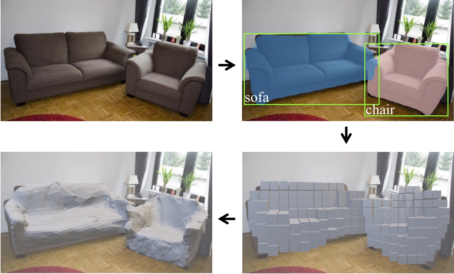
We believe that the time is ripe for these hitherto distinct research directions to be combined. We should strive to build systems that (like current methods for 2D perception) can operate on unconstrained real-world images with many objects, occlusion, and diverse lighting conditions but that (like current methods for 3D shape prediction) do not ignore the rich 3D structure of the world.

In this paper we take an initial step toward this goal. We draw on state-of-the-art methods for 2D perception and 3D shape prediction to build a system which inputs a real-world RGB image, detects the objects in the image, and outputs a category label, segmentation mask, and a 3D triangle mesh giving the full 3D shape of each detected object.

Our method, called Mesh R-CNN, builds on the state-of-the-art Mask R-CNN [18] system for 2D recognition, augmenting it with a mesh prediction branch that outputs high-resolution triangle meshes.

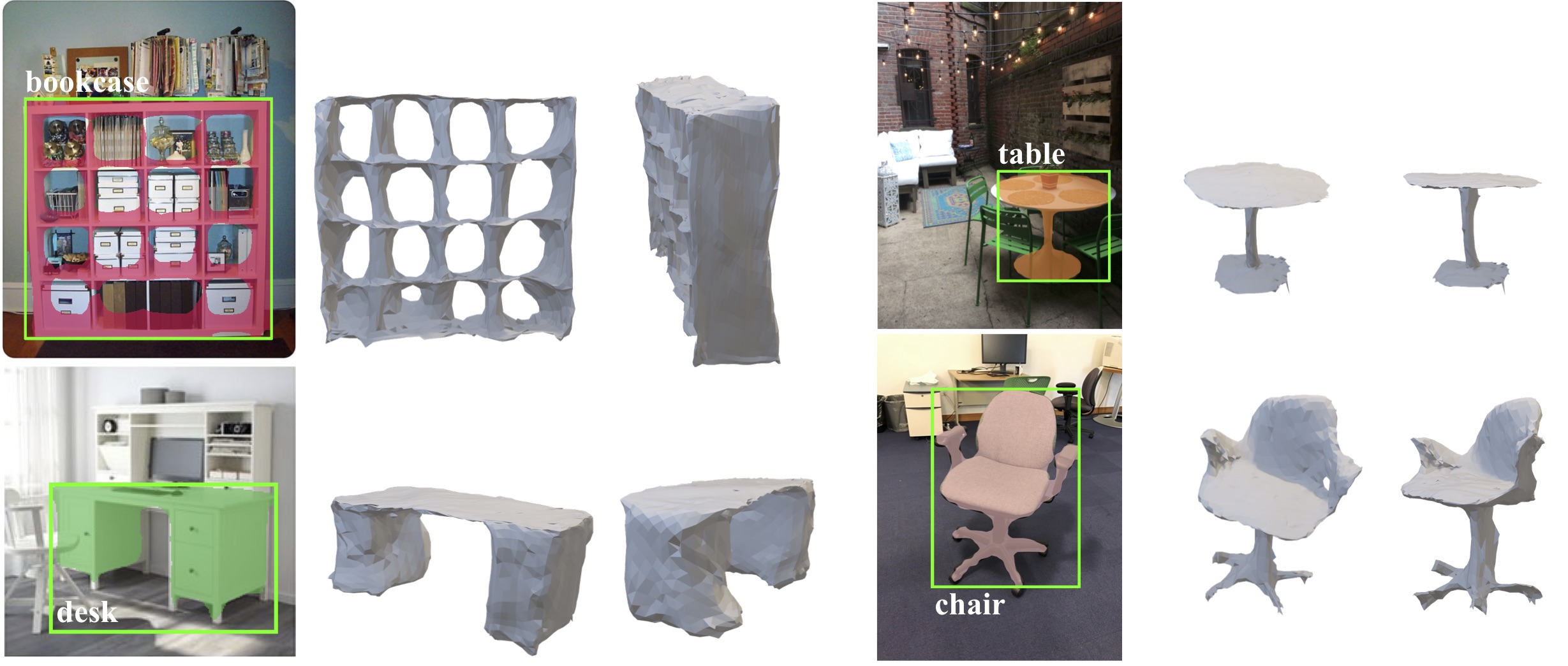
Our predicted meshes must be able to capture the 3D structure of diverse, real-world objects. Predicted meshes should therefore dynamically vary their complexity, topology, and geometry in response to varying visual stimuli. However, prior work on mesh prediction with deep networks [23, 57, 69] has been constrained to deform from fixed mesh templates, limiting them to fixed mesh topologies. As shown in Figure 1, we overcome this limitation by utilizing multiple 3D shape representations: we first predict coarse voxelized object representations, which are converted to meshes and refined to give highly accurate mesh predictions. As shown in Figure 2, this hybrid approach allows Mesh R-CNN to output meshes of arbitrary topology while also capturing fine object structures.

Figure 2: Example predictions from Mesh R-CNN on Pix3D. Using initial voxel predictions allows our outputs to vary in topology; converting these predictions to meshes and refining them allows us to capture fine structures like tabletops and chair legs.

We benchmark our approach on two datasets. First, we evaluate our mesh prediction branch on ShapeNet [4], where our hybrid approach of voxel prediction and mesh refinement outperforms prior work by a large margin. Second, we deploy our full Mesh R-CNN system on the recent Pix3D dataset [60] which aligns 395 models of IKEA furniture to real-world images featuring diverse scenes, clutter, and occlusion. To date Pix3D has primarily been used to evalute shape predictions for models trained on ShapeNet, using perfectly cropped, unoccluded image segments [41, 60, 73], or synthetic rendered images of Pix3D models [76]. In contrast, using Mesh R-CNN we are the first to train a system on Pix3D which can jointly detect objects of all categories and estimate their full 3D shape.

2 Related Work

Our system inputs a single RGB image and outputs a set of detected object instances, with a triangle mesh for each object. Our work is most directly related to recent advances in 2D object recognition and 3D shape prediction. We also draw more broadly from work on other 3D perception tasks.

2D Object Recognition Methods for 2D object recognition vary both in the type of information predicted per object, and in the overall system architecture. Object detectors output per-object bounding boxes and category labels [12, 13, 36, 38, 46, 47]; Mask R-CNN [18] additionally outputs instance segmentation masks. Our method extends this line of work to output a full 3D mesh per object.

Single-View Shape Prediction Recent approaches use a variety of shape representations for single-image 3D reconstruction. Some methods predict the orientation [10, 20] or 3D pose [31, 44, 66] of known shapes. Other approaches predict novel 3D shapes as sets of 3D points [8, 34], patches [15, 70], or geometric primitives [9, 64, 67]; others use deep networks to model signed distance functions [42]. These methods can flexibly represent complex shapes, but rely on post-processing to extract watertight mesh outputs.

Some methods predict regular voxel grids [5, 71, 72]; while intuitive, scaling to high-resolution outputs requires complex octree [50, 62] or nested shape architectures [49].

Others directly output triangle meshes, but are constrained to deform from fixed [56, 57, 69] or retrieved mesh templates [51], limiting the topologies they can represent.

Our approach uses a hybrid of voxel prediction and mesh deformation, enabling high-resolution output shapes that can flexibly represent arbitrary topologies.

Some methods reconstruct 3D shapes without 3D annotations [23, 25, 48, 68, 75]. This is an important direction, but at present we consider only the fully supervised case due to the success of strong supervision for 2D perception.

Multi-View Shape Prediction There is a broad line of work on multi-view reconstruction of objects and scenes, from classical binocular stereo [17, 53] to using shape priors [1, 2, 6, 21] and modern learning techniques [24, 26, 54]. In this work, we focus on single-image shape reconstruction.

3D Inputs Our method inputs 2D images and predicts semantic labels and 3D shapes. Due to the increasing availabilty of depth sensors, there has been growing interest in methods predicting semantic labels from 3D inputs such as RGB-D images [16, 58] and pointclouds [14, 32, 45, 59, 63]. We anticipate that incorporating 3D inputs into our method could improve the fidelity of our shape predictions.

Datasets Advances in 2D perception have been driven by large-scale annotated datasets such as ImageNet [52] and COCO [37]. Datasets for 3D shape prediction have lagged their 2D counterparts due to the difficulty of collecting 3D annotations. ShapeNet [4] is a large-scale dataset of CAD models which are rendered to give synthetic images. The IKEA dataset [33] aligns CAD models of IKEA objects to real-world images; Pix3D [60] extends this idea to a larger set of images and models. Pascal3D [74] aligns CAD models to real-world images, but it is unsuitable for shape reconstruction since its train and test sets share the same small set of models. KITTI [11] annotates outdoor street scenes with 3D bounding boxes, but does not provide shape annotations.

Figure 3: System overview of Mesh R-CNN. We augment Mask R-CNN with 3D shape inference. The voxel branch predicts a coarse shape for each detected object which is further deformed with a sequence of refinement stages in the mesh refinement branch.

3 Method

Our goal is to design a system that inputs a single image, detects all objects, and outputs a category label, bounding box, segmentation mask and 3D triangle mesh for each detected object. Our system must be able to handle cluttered real-world images, and must be trainable end-to-end. Our output meshes should not be constrained to a fixed topology in order to accommodate a wide variety of complex real-world objects. We accomplish these goals by marrying state-of-the-art 2D perception with 3D shape prediction.

Specifically, we build on Mask R-CNN [18], a state-of-the-art 2D perception system. Mask R-CNN is an end-to-end region-based object detector. It inputs a single RGB image and outputs a bounding box, category label, and segmentation mask for each detected object. The image is first passed through a backbone network (e.g. ResNet-50-FPN [35]); next a region proposal network (RPN)  [47] gives object proposals which are processed with object classification and mask prediction branches.

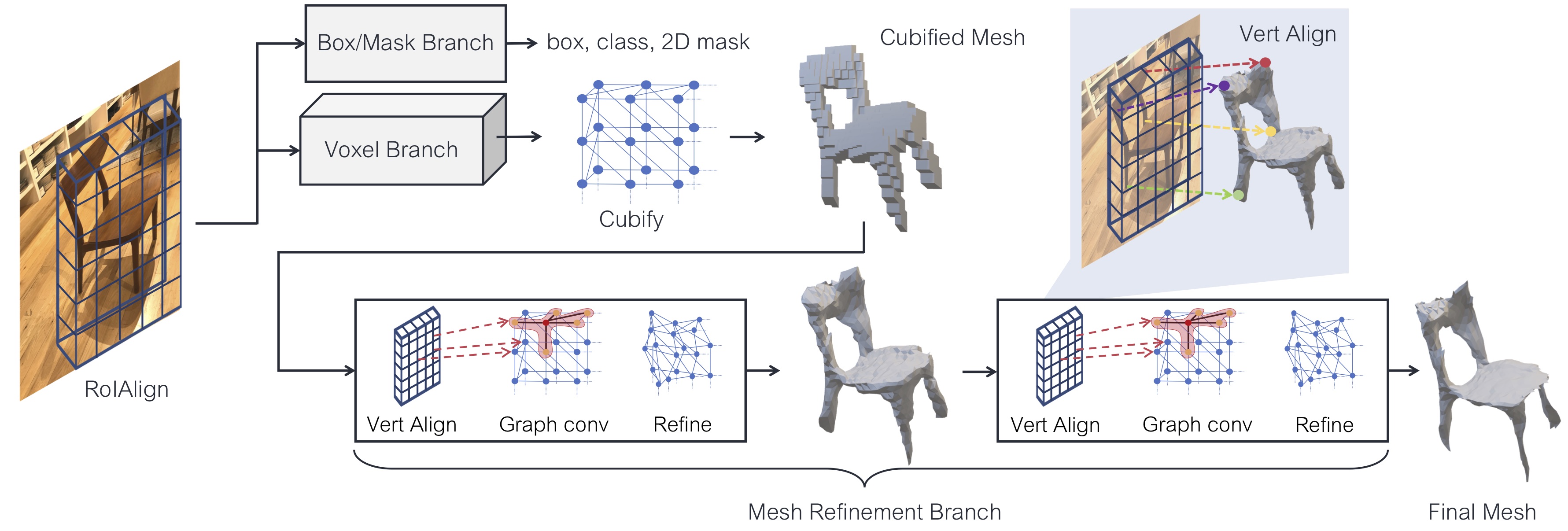
Part of Mask R-CNN’s success is due to RoIAlign which extracts region features from image features while maintaining alignment between the input image and features used in the final prediction branches. We aim to maintain similar feature alignment when predicting 3D shapes.

We infer 3D shapes with a novel mesh predictor, comprising a voxel branch and a mesh refinement branch. The voxel branch first estimates a coarse 3D voxelization of an object, which is converted to an initial triangle mesh. The mesh refinement branch then adjusts the vertex positions of this initial mesh using a sequence of graph convolution layers operating over the edges of the mesh.

The voxel branch and mesh refinement branch are homologous to the existing box and mask branches of Mask R-CNN. All take as input image-aligned features corresponding to RPN proposals. The voxel and mesh losses, described in detail below, are added to the box and mask losses and the whole system is trained end-to-end. The output is a set of boxes along with their predicted object scores, masks and 3D shapes. We call our system Mesh R-CNN, which is illustrated in Figure 3.

We now describe our mesh predictor, consisting of the voxel branch and mesh refinement branch, along with its associated losses in detail.

3.1 Mesh Predictor

At the core of our system is a mesh predictor which receives convolutional features aligned to an object’s bounding box and predicts a triangle mesh giving the object’s full 3D shape. Like Mask R-CNN, we maintain correspondence between the input image and features used at all stages of processing via region- and vertex-specific alignment operators (RoIAlign and VertAlign). Our goal is to capture instance-specific 3D shapes of all objects in an image. Thus, each predicted mesh must have instance-specific topology (genus, number of vertices, faces, connected components) and geometry (vertex positions).

We predict varying mesh topologies by deploying a sequence of shape inference operations. First, the voxel branch makes bottom-up voxelized predictions of each object’s shape, similar to Mask R-CNN’s mask branch. These predictions are converted into meshes and adjusted by the mesh refinement head, giving our final predicted meshes.

The output of the mesh predictor is a triangle mesh $T\!=\!(V,F)$ for each object. $V\!=\!\{v_{i}\!\in\!\mathbb{R}^{3}\}$ is the set of vertex positions and $F\!\subseteq\!V\times V\times V$ is a set of triangular faces.

3.1.1 Voxel Branch

The voxel branch predicts a grid of voxel occupancy probabilities giving the course 3D shape of each detected object. It can be seen as a 3D analogue of Mask R-CNN’s mask prediction branch: rather than predicting a $M\times M$ grid giving the object’s shape in the image plane, we instead predict a $G\times G\times G$ grid giving the object’s full 3D shape.

Like Mask R-CNN, we maintain correspondence between input features and predicted voxels by applying a small fully-convolutional network [39] to the input feature map resulting from RoIAlign. This network produces a feature map with $G$ channels giving a column of voxel occupancy scores for each position in the input.

Maintaining pixelwise correspondence between the image and our predictions is complex in 3D since objects become smaller as they recede from the camera. As shown in Figure 4, we account for this by using the camera’s (known) intrinsic matrix to predict frustum-shaped voxels.

World Space

Prediction Space

Figure 4: Predicting voxel occupancies aligned to the image plane requires an irregularly-shaped voxel grid. We achieve this effect by making voxel predictions in a space that is transformed by the camera’s (known) intrinsic matrix $K$. Applying $K^{-1}$ transforms our predictions back to world space. This results in frustum-shaped voxels in world space.

Cubify: Voxel to Mesh The voxel branch produces a 3D grid of occupancy probabilities giving the coarse shape of an object. In order to predict more fine-grained 3D shapes, we wish to convert these voxel predictions into a triangle mesh which can be passed to the mesh refinement branch.

We bridge this gap with an operation called cubify. It inputs voxel occupancy probabilities and a threshold for binarizing voxel occupancy. Each occupied voxel is replaced with a cuboid triangle mesh with 8 vertices, 18 edges, and 12 faces. Shared vertices and edges between adjacent occupied voxels are merged, and shared interior faces are eliminated. This results in a watertight mesh whose topology depends on the voxel predictions.

Cubify must be efficient and batched. This is not trivial and we provide technical implementation details of how we achieve this in Appendix A. Alternatively marching cubes [40] could extract an isosurface from the voxel grid, but is significantly more complex.

Voxel Loss The voxel branch is trained to minimize the binary cross-entropy between predicted voxel occupancy probabilities and true voxel occupancies.

3.1.2 Mesh Refinement Branch

The cubified mesh from the voxel branch only provides a coarse 3D shape, and it cannot accurately model fine structures like chair legs. The mesh refinement branch processes this initial cubified mesh, refining its vertex positions with a sequence of refinement stages. Similar to [69], each refinement stage consists of three operations: vertex alignment, which extracts image features for vertices; graph convolution, which propagates information along mesh edges; and vertex refinement, which updates vertex positions. Each layer of the network maintains a 3D position $v_{i}$ and a feature vector $f_{i}$ for each mesh vertex.

Vertex Alignment yields an image-aligned feature vector for each mesh vertex. We use the camera’s intrinsic matrix to project each vertex onto the image plane. Given a feature map, we compute a bilinearly interpolated image feature at each projected vertex position [22].

In the first stage of the mesh refinement branch, VertAlign outputs an initial feature vector for each vertex. In subsequent stages, the VertAlign output is concatenated with the vertex feature from the previous stage.

Graph Convolution [29] propagates information along mesh edges. Given input vertex features $\{f_{i}\}$ it computes updated features $\small f_{i}^{\prime}=\operatorname{ReLU}\big{(}W_{0}f_{i}+\sum_{j\in\mathcal{N}(i)}W_{1}f_{j}\big{)}$ where $\mathcal{N}(i)$ gives the $i$-th vertex’s neighbors in the mesh, and $W_{0}$ and $W_{1}$ are learned weight matrices. Each stage of the mesh refinement branch uses several graph convolution layers to aggregate information over local mesh regions.

Vertex Refinement computes updated vertex positions $v_{i}^{\prime}=v_{i}+\tanh(W_{vert}\left[f_{i};v_{i}\right])$ where $W_{vert}$ is a learned weight matrix. This updates the mesh geometry, keeping its topology fixed. Each stage of the mesh refinement branch terminates with vertex refinement, producing an intermediate mesh output which is further refined by the next stage.

Mesh Losses Defining losses that operate natively on triangle meshes is challenging, so we instead use loss functions defined over a finite set of points. We represent a mesh with a pointcloud by densely sampling its surface. Consequently, a pointcloud loss approximates a loss over shapes.

Similar to [57], we use a differentiable mesh sampling operation to sample points (and their normal vectors) uniformly from the surface of a mesh. To this end, we implement an efficient batched sampler; see Appendix B for details. We use this operation to sample a pointcloud $P^{gt}$ from the ground-truth mesh, and a pointcloud $P^{i}$ from each intermediate mesh prediction from our model.

Given two pointclouds $P$, $Q$ with normal vectors, let $\Lambda_{P,Q}=\{(p,\arg\min_{q}\|p-q\|):p\in P\}$ be the set of pairs $(p,q)$ such that $q$ is the nearest neighbor of $p$ in $Q$, and let $u_{p}$ be the unit normal to point $p$. The chamfer distance between pointclouds $P$ and $Q$ is given by

$$\footnotesize\mathcal{L}_{\textrm{cham}}(P,Q)=|P|^{-1}\sum_{(p,q)\in\Lambda_{P,Q}}\|p-q\|^{2}+|Q|^{-1}\sum_{(q,p)\in\Lambda_{Q,P}}\|q-p\|^{2}$$ (1)

and the (absolute) normal distance is given by

$$\footnotesize\mathcal{L}_{\textrm{norm}}(P,Q)=-|P|^{-1}\sum_{(p,q)\in\Lambda_{P,Q}}|u_{p}\cdot u_{q}|-|Q|^{-1}\sum_{(q,p)\in\Lambda_{Q,P}}|u_{q}\cdot u_{p}|.$$ (2)

The chamfer and normal distances penalize mismatched positions and normals between two pointclouds, but minimizing these distances alone results in degenerate meshes (see Figure 5). High-quality mesh predictions require additional shape regularizers: To this end we use an edge loss $\mathcal{L}_{\textrm{edge}}(V,E)=\frac{1}{|E|}\sum_{(v,v^{\prime})\in E}\|v-v^{\prime}\|^{2}$ where $E\subseteq V\times V$ are the edges of the predicted mesh. Alternatively, a Laplacian loss [7] also imposes smoothness constraints.

The mesh loss of the $i$-th stage is a weighted sum of $\mathcal{L}_{\textrm{cham}}(P^{i},P^{gt})$, $\mathcal{L}_{\textrm{norm}}(P^{i},P^{gt})$ and $\mathcal{L}_{\textrm{edge}}(V^{i},E^{i})$. The mesh refinement branch is trained to minimize the mean of these losses across all refinement stages.

4 Experiments

We benchmark our mesh predictor on ShapeNet [4], where we compare with state-of-the-art approaches. We then evaluate our full Mesh R-CNN for the task of 3D shape prediction in the wild on the challenging Pix3D dataset [60].

4.1 ShapeNet

ShapeNet [4] provides a collection of 3D shapes, represented as textured CAD models organized into semantic categories following WordNet [43], and has been widely used as a benchmark for 3D shape prediction. We use the subset of ShapeNetCore.v1 and rendered images from [5]. Each mesh is rendered from up to 24 random viewpoints, giving RGB images of size $137\times 137$. We use the train / test splits provided by [69], which allocate 35,011 models (840,189 images) to train and 8,757 models (210,051 images) to test; models used in train and test are disjoint. We reserve 5% of the training models as a validation set.

The task on this dataset is to input a single RGB image of a rendered ShapeNet model on a blank background, and output a 3D mesh for the object in the camera coordinate system. During training the system is supervised with pairs of images and meshes.

Evaluation We adopt evaluation metrics used in recent work [56, 57, 69]. We sample 10k points uniformly at random from the surface of predicted and ground-truth meshes, and use them to compute Chamfer distance (Equation 1), Normal consistency, (one minus Equation 2), and F1^τ at various distance thresholds $\tau$, which is the harmonic mean of the precision at $\tau$ (fraction of predicted points within $\tau$ of a ground-truth point) and the recall at $\tau$ (fraction of ground-truth points within $\tau$ of a predicted point). Lower is better for Chamfer distance; higher is better for all other metrics.

With the exception of normal consistency, these metrics depend on the absolute scale of the meshes. In Table 1 we follow [69] and rescale by a factor of 0.57; for all other results we follow [8] and rescale so the longest edge of the ground-truth mesh’s bounding box has length 10.

	Chamfer ($\downarrow$)	F1τ ($\uparrow$)	F12τ ($\uparrow$)
N3MR [25]	2.629	33.80	47.72
3D-R2N2 [5]	1.445	39.01	54.62
PSG [8]	0.593	48.58	69.78
Pixel2Mesh [69]†	0.591	59.72	74.19
MVD [56]	-	66.39	-
GEOMetrics [57]	-	67.37	-
Pixel2Mesh [69]‡	0.463	67.89	79.88
Ours (Best)	0.306	74.84	85.75
Ours (Pretty)	0.391	69.83	81.76

Table 1: Single-image shape reconstruction results on ShapeNet, using the evaluation protocol from [69]. For [69], ^† are results reported in their paper and ^‡ is the model released by the authors.

Implementation Details Our backbone feature extractor is ResNet-50 pretrained on ImageNet. Since images depict a single object, the voxel branch receives the entire conv5_3 feature map, bilinearly resized to $24\times 24$, and predicts a $48\times 48\times 48$ voxel grid. The VertAlign operator concatenates features from conv2_3, conv3_4, conv4_6, and conv5_3 before projecting to a vector of dimension 128. The mesh refinement branch has three stages, each with six graph convolution layers (of dimension 128) organized into three residual blocks. We train for 25 epochs using Adam [27] with learning rate $10^{-4}$ and 32 images per batch on 8 Tesla V100 GPUs. We set the cubify threshold to 0.2 and weight the losses with $\lambda_{\textrm{voxel}}=1$, $\lambda_{\textrm{cham}}=1$, $\lambda_{\textrm{norm}}=0$, and $\lambda_{\textrm{edge}}=0.2$.

Baselines We compare with previously published methods for single-image shape prediction. N3MR [25] is a weakly supervised approach that fits a mesh via a differentiable renderer without 3D supervision. 3D-R2N2 [5] and MVD [56] output voxel predictions. PSG [8] predicts point-clouds. Appendix D additionally compares with OccNet [42].

Pixel2Mesh [69] predicts meshes by deforming and subdividing an initial ellipsoid. GEOMetrics [57] extends [69] with adaptive face subdivision. Both are trained to minimize Chamfer distances; however [69] computes it using predicted mesh vertices, while [57] uses points sampled uniformly from predicted meshes. We adopt the latter as it better matches test-time evaluation. Unlike ours, these methods can only predict connected meshes of genus zero.

		Full Test Set							Holes Test Set
		Chamfer($\downarrow$)	Normal	F10.1	F10.3	F10.5	$|V|$	$|F|$	Chamfer($\downarrow$)	Normal	F10.1	F10.3	F10.5	$|V|$	$|F|$
	Pixel2Mesh [69]‡	0.205	0.736	33.7	80.9	91.7	2466 $\pm 0$	4928 $\pm 0$	0.272	0.689	31.5	75.9	87.9	2466 $\pm 0$	4928 $\pm 0$
	Voxel-Only	0.916	0.595	7.7	33.1	54.9	1987 $\pm 936$	3975 $\pm 1876$	0.760	0.592	8.2	35.7	59.5	2433 $\pm 925$	4877 $\pm 1856$
Best	Sphere-Init	0.132	0.711	38.3	86.5	95.1	2562 $\pm 0$	5120 $\pm 0$	0.138	0.705	40.0	85.4	94.3	2562 $\pm 0$	5120 $\pm 0$
	Pixel2Mesh+	0.132	0.707	38.3	86.6	95.1	2562 $\pm 0$	5120 $\pm 0$	0.137	0.696	39.3	85.5	94.4	2562 $\pm 0$	5120 $\pm 0$
	Ours (light)	0.133	0.725	39.2	86.8	95.1	1894 $\pm 925$	3791 $\pm 1855$	0.130	0.723	41.6	86.7	94.8	2273 $\pm 899$	4560 $\pm 1805$
	Ours	0.133	0.729	38.8	86.6	95.1	1899 $\pm 928$	3800 $\pm 1861$	0.130	0.725	41.7	86.7	94.9	2291 $\pm 903$	4595 $\pm 1814$
Pretty	Sphere-Init	0.175	0.718	34.5	82.2	92.9	2562 $\pm 0$	5120 $\pm 0$	0.186	0.684	34.4	80.2	91.7	2562 $\pm 0$	5120 $\pm 0$
	Pixel2Mesh+	0.175	0.727	34.9	82.3	92.9	2562 $\pm 0$	5120 $\pm 0$	0.196	0.685	34.4	79.9	91.4	2562 $\pm 0$	5120 $\pm 0$
	Ours (light)	0.176	0.699	34.8	82.4	93.1	1891 $\pm 924$	3785 $\pm 1853$	0.178	0.688	36.3	82.0	92.4	2281 $\pm 895$	4576 $\pm 1798$
	Ours	0.171	0.713	35.1	82.6	93.2	1896 $\pm 928$	3795 $\pm 1861$	0.171	0.700	37.1	82.4	92.7	2292 $\pm 902$	4598 $\pm 1812$

Table 2: We report results both on the full ShapeNet test set (left), as well as a subset of the test set consisting of meshes with visible holes (right). We compare our full model with several ablated version: Voxel-Only omits the mesh refinement head, while Sphere-Init and Pixel2Mesh⁺ omit the voxel head. We show results both for Best models which optimize for metrics, as well as Pretty models that strike a balance between shape metrics and mesh quality (see Figure 5); these two categories of models should not be compared. We also report the number of vertices $|V|$ and faces $|F|$ in predicted meshes (mean${}_{\pm\textrm{std}}$). ^‡ refers to the released model by the authors. (per-instance average)

The training recipe and backbone architecture vary among prior work. Therefore for a fair comparison with our method we also compare against several ablated versions of our model (see Appendix C for exact details):

• Voxel-Only: A version of our method that terminates with the cubified meshes from the voxel branch.

• Pixel2Mesh⁺: We reimplement Pixel2Mesh [69]; we outperform their original model due to a deeper backbone, better training recipe, and minimizing Chamfer on sampled rather than vertex positions.

• Sphere-Init: Similar to Pixel2Mesh⁺, but initializes from a high-resolution sphere mesh, performing three stages of vertex refinement without subdivision.

• Ours (light): Uses a smaller nonresidual mesh refinement branch with three graph convolution layers per stage. We will adopt this lightweight design on Pix3D.

Voxel-Only is essentially a version of our method that omits the mesh refinement branch, while Pixel2Mesh⁺ and Sphere-Init omit the voxel prediction branch.

Input Image

Without $\mathcal{L}_{edge}$ (best)

With $\mathcal{L}_{edge}$ (pretty)

Figure 5: Training without the edge length regularizer $\mathcal{L}_{edge}$ results in degenerate predicted meshes that have many overlapping faces. Adding $\mathcal{L}_{edge}$ eliminates this degeneracy but results in worse agreement with the ground-truth as measured by standard metrics such as Chamfer distance.

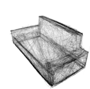
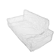
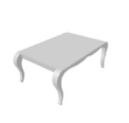
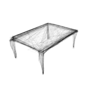
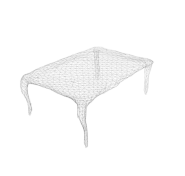
Best vs Pretty As previously noted in [69] (Section 4.1), standard metrics for shape reconstruction are not well-correlated with mesh quality. Figure 5 shows that models trained without shape regularizers give meshes that are preferred by metrics despite being highly degenerate, with irregularly-sized faces and many self-intersections. These degenerate meshes would be difficult to texture, and may not be useful for downstream applications.

Due to the strong effect of shape regularizers on both mesh quality and quantitative metrics, we suggest only quantitatively comparing methods trained with the same shape regularizers. We thus train two versions of all our ShapeNet models: a Best version with $\lambda_{\textrm{edge}}=0$ to serve as an upper bound on quantitative performance, and a Pretty version that strikes a balance between quantitative performance and mesh quality by setting $\lambda_{\textrm{edge}}=0.2$.

Comparison with Prior Work Table 1 compares our Pretty and Best models with prior work on shape prediction from a single image. We use the evaluation protocol from [69], using a 0.57 mesh scaling factor and threshold value $\tau=10^{-4}$ on squared Euclidean distances. For Pixel2Mesh, we provide the performance reported in their paper [69] as well as the performance of their open-source pretrained model. Table 1 shows that we outperform prior work by a wide margin, validating the design of our mesh predictor.

Pix3D $\mathcal{S}_{1}$	AP${}^{\text{box}}$	AP${}^{\text{mask}}$	AP${}^{\text{mesh}}$	chair	sofa	table	bed	desk	bkcs	wrdrb	tool	misc	$|V|$	$|F|$
Voxel-Only	94.4	88.4	5.3	0.0	3.5	2.6	0.5	0.7	34.3	5.7	0.0	0.0	$2354_{\pm 706}$	$4717_{\pm 1423}$
Pixel2Mesh+	93.5	88.4	39.9	30.9	59.1	40.2	40.5	30.2	50.8	62.4	18.2	26.7	$2562_{\pm 0}$	$5120_{\pm 0}$
Sphere-Init	94.1	87.5	40.5	40.9	75.2	44.2	50.3	28.4	48.6	42.5	26.9	7.0	$2562_{\pm 0}$	$5120_{\pm 0}$
Mesh R-CNN (ours)	94.0	88.4	51.1	48.2	71.7	60.9	53.7	42.9	70.2	63.4	21.6	27.8	$2367_{\pm 698}$	$4743_{\pm 1406}$
# test instances	2530	2530	2530	1165	415	419	213	154	79	54	11	20
Pix3D $\mathcal{S}_{2}$
Voxel-Only	71.5	63.4	4.9	0.0	0.1	2.5	2.4	0.8	32.2	0.0	6.0	0.0	$2346_{\pm 630}$	$4702_{\pm 1269}$
Pixel2Mesh+	71.1	63.4	21.1	26.7	58.5	10.9	38.5	7.8	34.1	3.4	10.0	0.0	$2562_{\pm 0}$	$5120_{\pm 0}$
Sphere-Init	72.6	64.5	24.6	32.9	75.3	15.8	40.1	10.1	45.0	1.5	0.8	0.0	$2562_{\pm 0}$	$5120_{\pm 0}$
Mesh R-CNN (ours)	72.2	63.9	28.8	42.7	70.8	27.2	40.9	18.2	51.1	2.9	5.2	0.0	$2358_{\pm 633}$	$4726_{\pm 1274}$
# test instances	2356	2356	2356	777	504	392	218	205	84	134	22	20

Table 3: Performance on Pix3D $\mathcal{S}_{1}$ & $\mathcal{S}_{2}$. We report mean AP${}^{\text{box}}$, AP${}^{\text{mask}}$ and AP${}^{\text{mesh}}$, as well as per category AP${}^{\text{mesh}}$. All AP performances are in %. The Voxel-Only baseline outputs the cubified voxel predictions. The Sphere-Init and Pixel2Mesh⁺ baselines deform an initial sphere and thus are limited to making predictions homeomorphic to spheres. Our Mesh R-CNN is flexible and can capture arbitrary topologies. We outperform the baselines consistently while predicting meshes with fewer number of vertices and faces.

CNN init	# refine steps	AP${}^{\text{box}}$	AP${}^{\text{mask}}$	AP${}^{\text{mesh}}$
COCO	3	94.0	88.4	51.1
IN	3	93.1	87.0	48.4
COCO	2	94.6	88.3	49.3
COCO	1	94.2	88.9	48.6

Table 4: Ablations of Mesh R-CNN on Pix3D.

Image

Pixel2Mesh⁺

Ours

Figure 6: Pixel2Mesh⁺ predicts meshes by deforming an initial sphere, so it cannot properly model objects with holes. In contrast our method can model objects with arbitrary topologies.

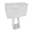
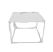
Ablation Study Fairly comparing with prior work is challenging due to differences in backbone networks, losses, and shape regularizers. For a controlled evaluation, we ablate variants using the same backbone and training recipe, shown in Table 2. ShapeNet is dominated by simple objects of genus zero. Therefore we evaluate both on the entire test set and on a subset consisting of objects with one or more holes (Holes Test Set) . In this evaluation we remove the ad-hoc scaling factor of 0.57, and we rescale meshes so the longest edge of the ground-truth mesh’s bounding box has length 10, following [8]. We compare the open-source Pixel2Mesh model against our ablations in this evaluation setting. Pixel2Mesh⁺ (our reimplementation of [69]) significantly outperforms the original due to an improved training recipe and deeper backbone.

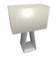
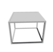
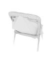
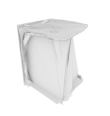
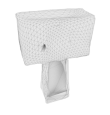
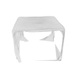
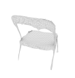
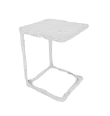
We draw several conclusions from Table 2: (a) On the Full Test Set, our full model and Pixel2Mesh⁺ perform on par. However, on the Holes Test Set, our model dominates as it is able to predict topologically diverse shapes while Pixel2Mesh⁺ is restricted to make predictions homeomorphic to spheres, and cannot model holes or disconnected components (see Figure 6). This discrepancy is quantitatively more salient on Pix3D (Section 4.2) as it contains more complex shapes. (b) Sphere-Init and Pixel2Mesh⁺ perform similarly overall (both Best and Pretty), suggesting that mesh subdivision may be unnecessary for strong quantitative performance. (c) The deeper residual mesh refinement architecture (inspired by [69]) performs on-par with the lighter non-residual architecture, motivating our use of the latter on Pix3D. (d) Voxel-Only performs poorly compared to methods that predict meshes, demonstrating that mesh predictions better capture fine object structure. (e) Each Best model outperforms its corresponding Pretty model; this is expected since Best is an upper bound on quantitative performance.

Figure 7: Examples of Mesh R-CNN predictions on Pix3D. Mesh R-CNN detects multiple objects per image, reconstructs fine details such as chair legs, and predicts varying and complex mesh topologies for objects with holes such as bookcases and tables.

4.2 Pix3D

We now turn to Pix3D [60], which consists of 10069 real-world images and 395 unique 3D models. Here the task is to jointly detect and predict 3D shapes for known object categories. Pix3D does not provide standard train/test splits, so we prepare two splits of our own.

Our first split, $\mathcal{S}_{1}$, randomly allocates 7539 images for training and 2530 for testing. Despite the small number of unique object models compared to ShapeNet, $\mathcal{S}_{1}$ is challenging since the same model can appear with varying appearance (e.g. color, texture), in different orientations, under different lighting conditions, in different contexts, and with varying occlusion. This is a stark contrast with ShapeNet, where objects appear against blank backgrounds.

Our second split, $\mathcal{S}_{2}$, is even more challenging: we ensure that the 3D models appearing in the train and test sets are disjoint. Success on this split requires generalization not only to the variations present in $\mathcal{S}_{1}$, but also to novel 3D shapes of known categories: for example a model may see kitchen chairs during training but must recognize armchairs during testing. This split is possible due to Pix3D’s unique annotation structure, and poses interesting challenges for both 2D recognition and 3D shape prediction.

Evaluation We adopt metrics inspired by those used for 2D recognition: AP${}^{\text{box}}$, AP${}^{\text{mask}}$ and AP${}^{\text{mesh}}$. The first two are standard metrics used for evaluating COCO object detection and instance segmentation at intersection-over-union (IoU) 0.5. AP${}^{\text{mesh}}$ evalutes 3D shape prediction: it is the mean area under the per-category precision-recall curves for F1^0.3 at 0.5. Pix3D is not exhaustively annotated, so for evaluation we only consider predictions with box $\textrm{IoU}>0.3$ with a ground-truth region. This avoids penalizing the model for correct predictions corresponding to unannotated objects.

We compare predicted and ground-truth meshes in the camera coordinate system. Our model assumes known camera intrinsics for VertAlign. In addition to predicting the box of each object on the image plane, Mesh R-CNN predicts the depth extent by appending a 2-layer MLP head, similar to the box regressor head. As a result, Mesh R-CNN predicts a 3D bounding box for each object. See Appendix E for more details.

Implementation details We use ResNet-50-FPN [35] as the backbone CNN; the box and mask branches are identical to Mask R-CNN. The voxel branch resembles the mask branch, but the pooling resolution is decreased to 12 (vs. 14 for masks) due to memory constraints giving $24\times 24\times 24$ voxel predictions. We adopt the lightweight design for the mesh refinement branch from Section 4.1. We train for 12 epochs with a batch size of 64 per image on 8 Tesla V100 GPUs (two images per GPU). We use SGD with momentum, linearly increasing the learning rate from $0.002$ to $0.02$ over the first 1K iterations, then decaying by a factor of 10 at 8K and 10K iterations. We initialize from a model pretrained for instance segmentation on COCO. We set the cubify threshold to $0.2$ and the loss weights to $\lambda_{\textrm{voxel}}=3$, $\lambda_{\textrm{cham}}=1$, $\lambda_{\textrm{norm}}=0.1$ and $\lambda_{\textrm{edge}}=1$ and use weight decay $10^{-4}$; detection loss weights are identical to Mask R-CNN.

Comparison to Baselines As discussed in Section 1, we are the first to tackle joint detection and shape inference in the wild on Pix3D. To validate our approach we compare with ablated versions of Mesh R-CNN, replacing our full mesh predictor with Voxel-Only, Pixel2Mesh⁺, and Sphere-Init branches (see Section 4.1). All baselines otherwise use the same architecture and training recipe.

Table 3 (top) shows the performance on $\mathcal{S}_{1}$. We observe that: (a) Mesh R-CNN outperforms all baselines, improving over the next-best by 10.6% AP${}^{\text{mesh}}$ overall and across most categories; Tool and Misc have very few test-set instances (11 and 20 respectively), so their AP is noisy. (b) Mesh R-CNN shows large gains vs. Sphere-Init for objects with complex shapes such as bookcase (+21.6%), table (+16.7%) and chair (+7.3%). (c) Voxel-Only performs very poorly – this is expected due to its coarse predictions.

Table 3 (bottom) shows the performance on the more challenging $\mathcal{S}_{2}$ split. Here we observe: (a) The overall performance on 2D recognition (AP${}^{\text{box}}$ , AP${}^{\text{mask}}$ ) drops significantly compared to $\mathcal{S}_{1}$, signifying the difficulty of recognizing novel shapes in the wild. (b) Mesh R-CNN outperforms all baselines for shape prediction for all categories except sofa, wardrobe and tool. (c) Absolute performance on wardrobe, tool and misc is small for all methods due to significant shape disparity between models in train and test and lack of training data.

Table 4 compares pretraining on COCO vs ImageNet, and compares different architectures for the mesh predictor. COCO vs. ImageNet initialization improves 2D recognition (AP${}^{\text{mask}}$ 88.4 vs. 87.0) and 3D shape prediction (AP${}^{\text{mesh}}$ 51.1 vs. 48.4). Shape prediction is degraded when using only one mesh refinement stage (AP${}^{\text{mesh}}$ 51.1 vs. 48.6).

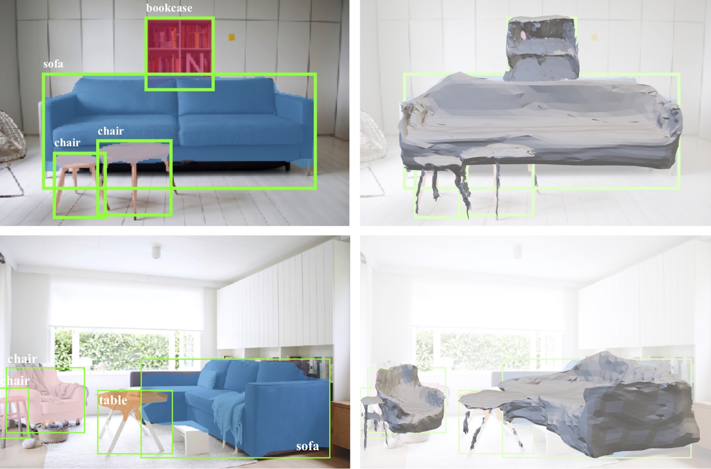
Figures 2, 7 and 8 show example predictions from Mesh R-CNN. Our method can detect multiple objects per image, reconstruct fine details such as chair legs, and predict varying and complex mesh topologies for objects with holes such as bookcases and desks.

Figure 8: More examples of Mesh R-CNN predictions on Pix3D.

Discussion

We propose Mesh R-CNN, a novel system for joint 2D perception and 3D shape inference. We validate our approach on ShapeNet and show its merits on Pix3D. Mesh R-CNN is a first attempt at 3D shape prediction in the wild. Despite the lack of large supervised data, e.g. compared to COCO, Mesh R-CNN shows promising results. Mesh R-CNN is an object centric approach. Future work includes reasoning about the 3D layout, i.e. the relative pose of objects in the 3D scene.

Acknowledgements We would like to thank Kaiming He, Piotr Dollár, Leonidas Guibas, Manolis Savva and Shubham Tulsiani for valuable discussions. We would also like to thank Lars Mescheder and Thibault Groueix for their help.

Appendix

Appendix A Implementation of Cubify

Algorithm 1 outlines the cubify operation. Cubify takes as input voxel occupancy probabilities $V$ of shape $N\times D\times H\times W$ as predicted from the voxel branch and a threshold value $\tau$. Each occupied voxel is replaced with a cuboid triangle mesh (unit_cube) with 8 vertices, 18 edges, and 12 faces. Shared vertices and edges between adjacent occupied voxels are merged, and shared interior faces are eliminated. This results in a watertight mesh $T=(V,F)$ for each example in the batch whose topology depends on the voxel predictions.

Algorithm 1 is an inefficient implementation of cubify as it involves nested for loops which in practice increase the time complexity, especially for large batches and large voxel sizes. In particular, this implementation takes $>$ 300ms for $N=32$ voxels of size $32\times 32\times 32$ on a Tesla V100 GPU. We replace the nested for loops with 3D convolutions and vectorize our computations, resulting in a time complexity of $\approx$ 30ms for the same voxel inputs.

Data: $V:[0,1]^{N\times D\times H\times W}$, $\tau\in[0,1]$

$\textrm{unit\_cube}=(V_{\textrm{cube}},F_{\textrm{cube}})$

for (n, z, y, x) $\in$ range(N, D, H, W) do

       if $V[n,z,y,x]>\tau$ then

             add unit_cube at $(n,z,y,x)$

             if $V[n,z-1,y,x]>\tau$ then

                   remove back faces

                  

             end if

            if $V[n,z+1,y,x]>\tau$ then

                   remove front faces

                  

             end if

            if $V[n,z,y-1,x]>\tau$ then

                   remove top faces

                  

             end if

            if $V[n,z,y+1,x]>\tau$ then

                   remove bottom faces

                  

             end if

            if $V[n,z,y,x-1]>\tau$ then

                   remove left faces

                  

             end if

            if $V[n,z,y,x+1]>\tau$ then

                   remove right faces

                  

             end if

            

       end if

      

end for

merge shared verts

return A list of meshes $\{T_{i}=(V_{i},F_{i})\}_{i=0}^{N-1}$

Algorithm 1 Cubify

Appendix B Mesh Sampling

As described in the main paper, the mesh refinement head is trained to minimize chamfer and normal losses that are defined on sets of points sampled from the predicted and ground-truth meshes.

Computing these losses requires some method of converting meshes into sets of sampled points. Pixel2Mesh [69] is trained using similar losses. In their case ground-truth meshes are represented with points sampled uniformly at random from the surface of the mesh, but this sampling is performed offline before the start of training; they represent predicted meshes using their vertex positions. Computing these losses using vertex positions of predicted meshes is very efficient since it avoids the need to sample meshes online during training; however it can lead to degenerate predictions since the loss would not encourage the interior of predicted faces to align with the ground-truth mesh.

To avoid these potential degeneracies, we follow [57] and compute the chamfer and normal losses by randomly sampling points from both the predicted and ground-truth meshes. This means that we need to sample the predicted meshes online during training, so the sampling must be efficient and we must be able to backpropagate through the sampling procedure to propagate gradients backward from the sampled points to the predicted vertex positions.

Given a mesh with vertices $V\subset\mathbb{R}^{3}$ and faces $F\subseteq V\times V\times V$, we can sample a point uniformly from the surface of the mesh as follows. We first define a probability distribution over faces where each face’s probability is proportional to its area:

$$P(f)=\frac{area(f)}{\sum_{f^{\prime}\in F}area(f^{\prime})}$$ (3)

We then sample a face $f=(v_{1},v_{2},v_{3})$ from this distribution. Next we sample a point $p$ uniformly from the interior of $f$ by setting $p=\sum_{i}w_{i}v_{i}$ where $w_{1}=1-\sqrt{\xi_{1}}$, $w_{2}=(1-\xi_{2})\sqrt{\xi}_{1}$, $w_{3}=\xi_{2}\sqrt{\xi}_{1}$, and $\xi_{1},\xi_{2}\sim U(0,1)$ are sampled from a uniform distribution.

This formulation allows propagating gradients from $p$ backward to the face vertices $v_{i}$ and can be seen as an instance of the reparameterization trick [28].

Appendix C Mesh R-CNN Architecture

At a high level we use the same overall architecture for predicting meshes on ShapeNet and Pix3D, but we slightly specialize to each dataset due to memory constraints from the backbone and task-specific heads. On Pix3D Mask R-CNN adds time and memory complexity in order to perform object detection and instance segmentation.

Index	Inputs	Operation	Output shape
(1)	Input	conv2_3 features	$35\times 35\times 256$
(2)	Input	conv3_4 features	$18\times 18\times 512$
(3)	Input	conv4_6 features	$9\times 9\times 1024$
(4)	Input	conv5_3 features	$5\times 5\times 2048$
(5)	Input	Input vertex features	$|V|\times 128$
(6)	Input	Input vertex positions	$|V|\times 3$
(7)	(1), (6)	VertAlign	$|V|\times 256$
(8)	(2), (6)	VertAlign	$|V|\times 512$
(9)	(3), (6)	VertAlign	$|V|\times 1024$
(10)	(4), (6)	VertAlign	$|V|\times 2048$
(11)	(7),(8),(9),(10)	Concatenate	$|V|\times 3840$
(12)	(11)	Linear$(3840\rightarrow 128)$	$|V|\times 128$
(13)	(5), (6), (12)	Concatenate	$|V|\times 259$
(14)	(13)	ResGraphConv$(259\rightarrow 128)$	$|V|\times 128$
(15)	(14)	$2\times$ ResGraphConv$(128\rightarrow 128)$	$|V|\times 128$
(16)	(15)	GraphConv$(128\rightarrow 3)$	$|V|\times 3$
(17)	(16)	Tanh	$|V|\times 3$
(18)	(6), (17)	Addition	$|V|\times 3$

Table 5: Architecture for a single residual mesh refinement stage on ShapeNet. For ShapeNet we follow [69] and use residual blocks of graph convolutions: ResGraphConv$(D_{1}\rightarrow D_{2})$ consists of two graph convolution layers (each preceeded by ReLU) and an additive skip connection, with a linear projection if the input and output dimensions are different. The output of the refinement stage are the vertex features (15) and the updated vertex positions (18). The first refinement stage does not take input vertex features (5), so for this stage (13) only concatenates (6) and (12).

Index	Inputs	Operation	Output shape
(1)	Input	Image	$137\times 137\times 3$
(2)	(1)	ResNet-50 conv2_3	$35\times 35\times 256$
(3)	(2)	ResNet-50 conv3_4	$18\times 18\times 512$
(4)	(3)	ResNet-50 conv4_6	$9\times 9\times 1024$
(5)	(4)	ResNet-50 conv5_3	$5\times 5\times 2048$
(6)	(5)	Bilinear interpolation	$24\times 24\times 2048$
(7)	(6)	Voxel Branch	$48\times 48\times 48$
(8)	(7)	cubify	$|V|\times 3,|F|\times 3$
(9)	(2), (3), (4), (5), (8)	Refinement Stage 1	$|V|\times 3,|F|\times 3$
(10)	(2), (3), (4), (5), (9)	Refinement Stage 2	$|V|\times 3,|F|\times 3$
(11)	(2), (3), (4), (5), (10)	Refinement Stage 3	$|V|\times 3,|F|\times 3$

Table 6: Overall architecture for our ShapeNet model. Since we do not predict bounding boxes or masks, we feed the conv5_3 features from the whole image into the voxel branch. The architecture for the refinement stage is shown in Table 5, and the architecture for the voxel branch is shown in Table 8.

ShapeNet. The overall architecture of our ShapeNet model is shown in Table 6; the architecture of the voxel branch is shown in Table 8.

We consider two different architectures for the mesh refinement network on ShapeNet. Our full model as well as our Pixel2Mesh⁺ and Sphere-Init baselines use mesh refinement stages with three residual blocks of two graph convolutions each, similar to [69]; the architecture of these stages is shown in Table 5. We also consider a shallower lightweight design which uses only three graph convolution layers per stage, omitting residual connections and instead concatenating the input vertex positions before each graph convolution layer. The architecture of this lightweight design is shown in Table 7.

As shown in Table 2, we found that these two architectures perform similarly on ShapeNet even though the lightweight design uses half as many graph convolution layers per stage. We therefore use the nonresidual design for our Pix3D models.

Pix3D. The overall architecture of our full Mesh R-CNN system on Pix3D is shown in Table 9. The backbone, RPN, box branch, and mask branch are identical to Mask R-CNN [18]. The voxel branch is the same as in the ShapeNet models (see Table 8), except that we predict voxels at a lower resolution ($48\times 48\times 48$ for ShapeNet vs. $24\times 24\times 24$ for Pix3D) due to memory constraints. Table 10 shows the exact architecture of the mesh refinement stages for our Pix3D models.

Index	Inputs	Operation	Output shape
(1)	Input	conv2_3 features	$35\times 35\times 256$
(2)	Input	conv3_4 features	$18\times 18\times 512$
(3)	Input	conv4_6 features	$9\times 9\times 1024$
(4)	Input	conv5_3 features	$5\times 5\times 2048$
(5)	Input	Input vertex features	$|V|\times 128$
(6)	Input	Input vertex positions	$|V|\times 3$
(7)	(1), (6)	VertAlign	$|V|\times 256$
(8)	(2), (6)	VertAlign	$|V|\times 512$
(9)	(3), (6)	VertAlign	$|V|\times 1024$
(10)	(4), (6)	VertAlign	$|V|\times 2048$
(11)	(7),(8),(9),(10)	Concatenate	$|V|\times 3840$
(12)	(11)	Linear$(3840\rightarrow 128)$	$|V|\times 128$
(13)	(5), (6), (12)	Concatenate	$|V|\times 259$
(14)	(13)	GraphConv$(259\rightarrow 128)$	$|V|\times 128$
(15)	(6), (14)	Concatenate	$|V|\times 131$
(16)	(15)	GraphConv$(131\rightarrow 128)$	$|V|\times 128$
(17)	(6), (16)	Concatenate	$|V|\times 131$
(18)	(17)	GraphConv$(131\rightarrow 128)$	$|V|\times 128$
(19)	(18)	Linear$(128\rightarrow 3)$	$|V|\times 3$
(20)	(19)	Tanh	$|V|\times 3$
(21)	(6), (20)	Addition	$|V|\times 3$

Table 7: Architecture for the nonresidual mesh refinement stage use in the lightweight version of our ShapeNet models. Each GraphConv operation is followed by ReLU. The output of the stage are the vertex features (18) and updated vertex positions (21). The first refinement stage does not take input vertex features (5), so for this stage (13) only concatenates (6) and (12).

Index	Inputs	Operation	Output shape
(1)	Input	Image features	$V/2\times V/2\times D$
(2)	(1)	Conv$(D\rightarrow 256,3\times 3)$, ReLU	$V/2\times V/2\times 256$
(3)	(2)	Conv$(256\rightarrow 256,3\times 3)$, ReLU	$V/2\times V/2\times 256$
(4)	(3)	TConv$(256\rightarrow 256,2\times 2,2)$, ReLU	$V\times V\times 256$
(5)	(4)	Conv$(256\rightarrow V,1\times 1)$	$V\times V\times V$

Table 8: Architecture of our voxel prediction branch. For ShapeNet we use $V=48$ and for Pix3D we use $V=24$. TConv is a transpose convolution with stride 2.

Baselines. The Voxel-Only baseline is identical to the full model, except that it omits all mesh refinement branches and terminates with the mesh resulting from cubify. On ShapeNet, the Voxel-Only baseline is trained with a batch size of 64 (vs. a batch size of 32 for our full model); on Pix3D it uses the same training recipe as our full model.

Index	Inputs	Operation	Output shape
(1)	Input	Input Image	$H\times W\times 3$
(2)	(1)	Backbone: ResNet-50-FPN	$h\times w\times 256$
(3)	(2)	RPN	$h\times w\times A\times 4$
(4)	(2),(3)	RoIAlign	$14\times 14\times 256$
(5)	(4)	Box branch: $2\times$ downsample, Flatten, Linear$(7*7*256\rightarrow 1024)$, Linear$(1024\rightarrow 5C)$	$C\times 5$
(6)	(4)	Mask branch: $4\times$ Conv$(256\rightarrow 256,3\times 3)$, TConv$(256\rightarrow 256,2\times 2,2)$, Conv($256\rightarrow C,1\times 1$)	$28\times 28\times C$
(7)	(2), (3)	RoIAlign	$12\times 12\times 256$
(8)	(7)	Voxel Branch	$24\times 24\times 24$
(9)	(8)	cubify	$|V|\times 3$, $|F|\times 3$
(10)	(7), (9)	Refinement Stage 1	$|V|\times 3$, $|F|\times 3$
(11)	(7), (10)	Refinement Stage 2	$|V|\times 3$, $|F|\times 3$
(12)	(7), (11)	Refinement Stage 3	$|V|\times 3$, $|F|\times 3$

Table 9: Overall architecture of Mesh R-CNN on Pix3D. The backbone, RPN, box, and mask branches are identical to Mask R-CNN. The RPN produces a bounding box prediction for each of the $A$ anchors at each spatial location in the input feature map; a subset of these candidate boxes are processed by the other branches, but here we show only the shapes resulting from processing a single box for the subsequent task-specific heads. Here $C$ is the number of categories (10 = 9 + background for Pix3D); the box branch produces per-category bounding boxes and classification scores, while the mask branch produces per-category segmentation masks. TConv is a transpose convolution with stride 2. We use a ReLU nonlinearity between all Linear, Conv, and TConv operations. The architecture fo the voxel branch is shown in Table 8, and the architecture of the refinement stages is shown in Table 10.

Index	Inputs	Operation	Output shape
(1)	Input	Backbone features	$h\times w\times 256$
(2)	Input	Input vertex features	$|V|\times 128$
(3)	Input	Input vertex positions	$|V|\times 3$
(4)	(1), (3)	VertAlign	$|V|\times 256$
(5)	(2), (3), (4)	Concatenate	$|V|\times 387$
(6)	(5)	GraphConv$(387\rightarrow 128)$	$|V|\times 128$
(7)	(3), (6)	Concatenate	$|V|\times 131$
(8)	(7)	GraphConv$(131\rightarrow 128)$	$|V|\times 128$
(9)	(3), (8)	Concatenate	$|V|\times 131$
(10)	(9)	GraphConv$(131\rightarrow 128)$	$|V|\times 128$
(11)	(3), (10)	Concatenate	$|V|\times 131$
(12)	(11)	Linear$(131\rightarrow 3)$	$|V|\times 3$
(13)	(12)	Tanh	$|V|\times 3$
(14)	(3), (13)	Addition	$|V|\times 3$

Table 10: Architecture for a single mesh refinement stage on Pix3D.

The Pixel2Mesh⁺ is our reimplementation of [69]. This baseline omits the voxel branch; instead all images use an identical inital mesh. The initial mesh is a level-2 icosphere with 162 vertices, 320 faces, and 480 edges which results from applying two face subdivision operations to a regular icosahedron and projecting all resulting vertices onto a sphere. For the Pixel2Mesh⁺ baseline, the mesh refinement stages are the same as our full model, except that we apply a face subdivision operation prior to VertAlign in refinement stages 2 and 3.

Like Pixel2Mesh⁺, the Sphere-Init baseline omits the voxel branch and uses an identical initial sphere mesh for all images. However unlike Pixel2Mesh⁺ the initial mesh is a level-4 icosphere with 2562 vertices, 5120 faces, and 7680 edges which results from applying four face subdivivison operations to a regular icosahedron. Due to this large initial mesh, the mesh refinement stages are identical to our full model, and do not use mesh subdivision.

Pixel2Mesh⁺ and Sphere-Init both predict meshes with the same number of vertices and faces, and with identical topologies; the only difference between them is whether all subdivision operations are performed before the mesh refinement branch (Sphere-Init) or whether mesh refinement is interleaved with mesh subdivision (Pixel2Mesh⁺). On ShapeNet, the Pixel2Mesh⁺ and Sphere-Init baselines are trained with a batch size of 96; on Pix3D they use the same training recipe as our full model.

		Chamfer($\downarrow$)	Normal	F10.1	F10.3	F10.5	$|V|$	$|F|$
	OccNet [42]	0.264	0.789	33.4	80.5	91.3	2499 $\pm 60$	4995 $\pm 120$
Best	Ours (light)	0.135	0.725	38.9	86.7	95.0	1978 $\pm 951$	3958 $\pm 1906$
	Ours	0.139	0.728	38.3	86.3	94.9	1985 $\pm 960$	3971 $\pm 1924$
Pretty	Ours (light)	0.185	0.696	34.3	82.0	92.8	1976 $\pm 956$	3954 $\pm 1916$
	Ours	0.180	0.709	34.6	82.2	93.0	1982 $\pm 961$	3967 $\pm 1926$

Table 11: Comparison between our method and Occpancy Networks (OccNet) [42] on ShapeNet. We use the same evaluation metrics and setup as Table 2.

Appendix D Comparison with Occupancy Networks

Occupancy Networks [42] (OccNet) also predict 2D meshes with neural networks. Rather than outputing a mesh directly from the neural network as in our approach, they train a neural network to compute a signed distance between a query point in 3D space and the object boundary. At test-time a 3D mesh can be extracted from a set of query points. Like our approach, OccNets can also predict meshes with varying topolgy per input instance.

Table 11 compares our approach with OccNet on the ShapeNet test set. We obtained test-set predictions for OccNet from the authors. Our method and OccNet are trained on slightly different splits of the ShapeNet dataset, so we compare our methods on the intersection of our respective test splits. From Table 11 we see that OccNets achieve higher normal consistency than our approach; however both the Best and Pretty versions of our model outperform OccNets on all other metrics.

Appendix E Depth Extent Prediction

Predicting an object’s depth extent from a single image is an ill-posed problem. In an earlier version of our work, we assumed the range of an object in the $Z$-axis was given at train & test time. Since then, we have attempted to predict the depth extent by training a 2-layer MLP head of similar architecture to the bounding box regressor head. Formally, this head is trained to predict the scale-normalized depth extent (in $\log$ space) of the object, as follows

$$\bar{dz}=\frac{dz}{z_{c}}\cdot\frac{f}{h}$$ (4)

Note that the depth extent of an object is related to the size of the object (here approximated by the object’s bounding box height $h$), its location $z_{c}$ in the $Z$-axis (far away objects need to be bigger in order to explain the image) and the focal length $f$. At inference time the depth extent $dz$ of the object is recovered from the predicted $\bar{dz}$ and the predicted height of the object bounding box $h$, given the focal length $f$ and the center of the object $z_{c}$ in the $Z$-axis. Note that we assume the center of the object $z_{c}$ since Pix3D annotations are not metric and due to the inherent scale-depth ambiguity.

Appendix F Pix3D: Visualizations and Comparisons

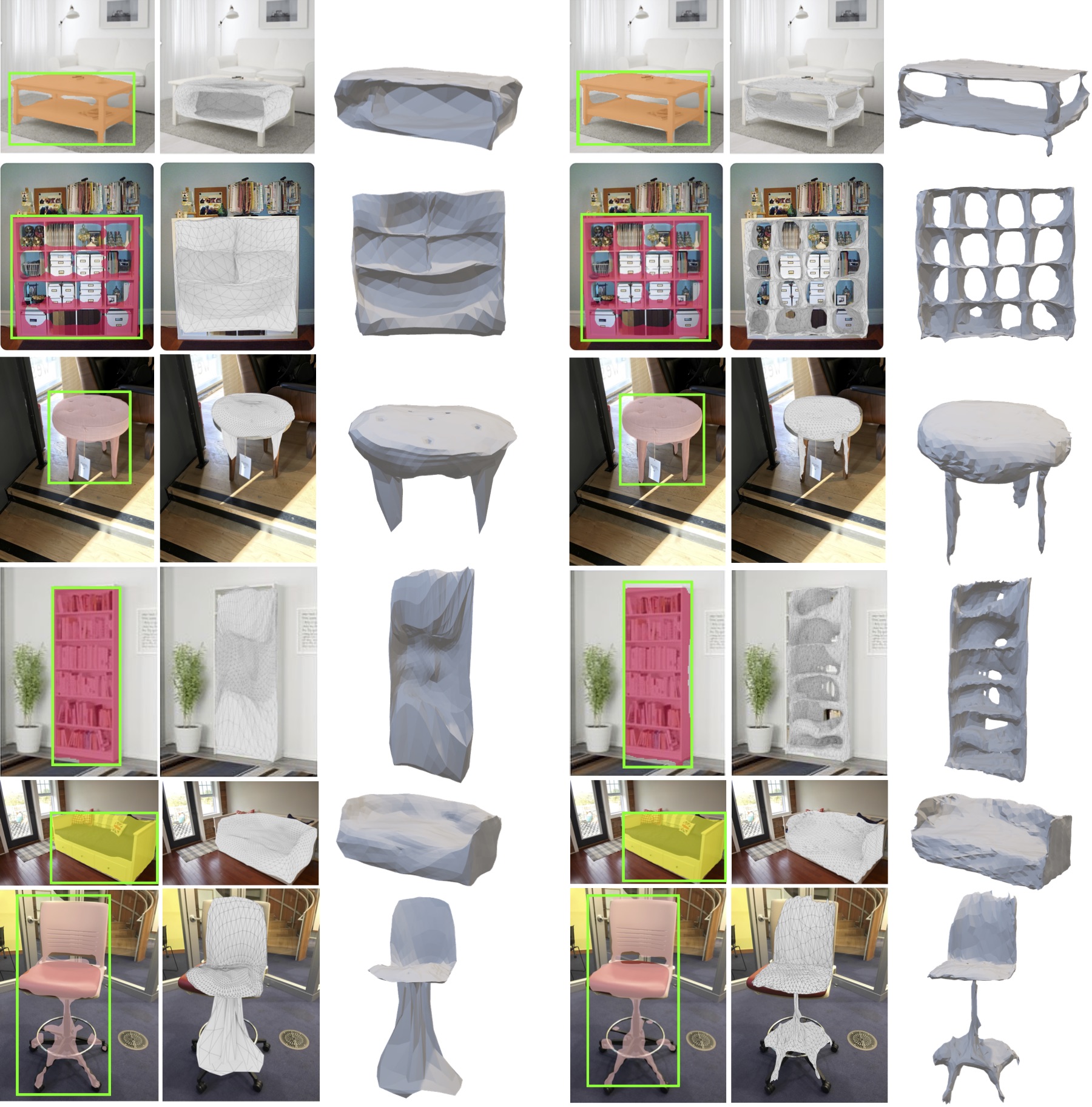
Figure 9 shows qualitative comparisons between Pixel2Mesh⁺ and Mesh R-CNN. Pixel2Mesh⁺ is limited to making predictions homeomorphic to spheres and thus cannot capture varying topologies, e.g. holes. In addition, Pixel2Mesh⁺ has a hard time capturing high curvatures, such as sharp table tops and legs. This is due to the large deformations required when starting from a sphere, which are not encouraged by the shape regularizers. On the other hand, Mesh R-CNN initializes its shapes with cubified voxel predictions resulting in better initial shape representations which require less drastic deformations.

Pixel2Mesh⁺                     Mesh R-CNN

Figure 9: Qualitative comparisons between Pixel2Mesh⁺ and Mesh R-CNN on Pix3D. Each row shows the same example for Pixel2Mesh⁺ (first three columns) and Mesh R-CNN (last three columns), respectively. For each method, we show the input image along with the predicted 2D mask ( chair, bookcase, table, bed) and box (in green) superimposed. We show the 3D mesh rendered on the input image and an additional view of the 3D mesh.

Appendix G ShapeNet Holes test set

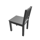
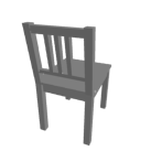
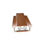
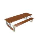
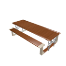
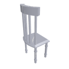
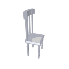
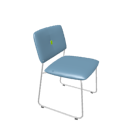
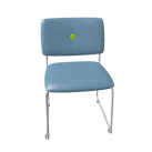
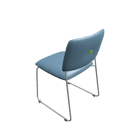
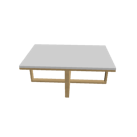
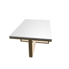
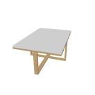
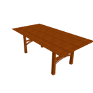
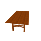
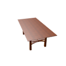
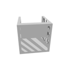
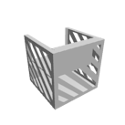
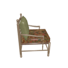
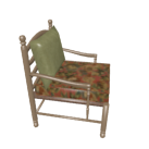
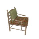
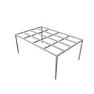
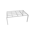
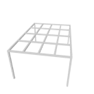
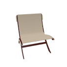
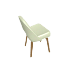
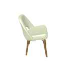
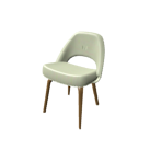
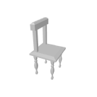
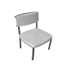
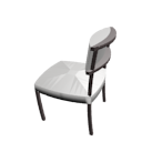
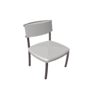
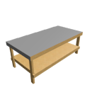
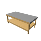
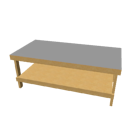
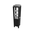
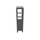
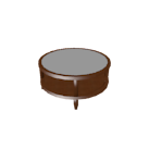
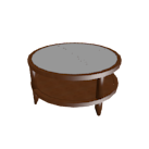
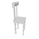
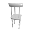
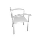
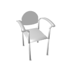
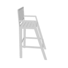
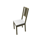
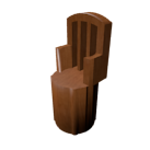
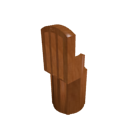
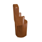
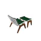
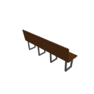
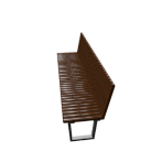
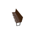
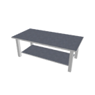
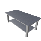
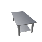
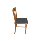
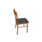
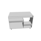
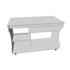
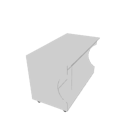
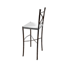
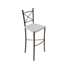
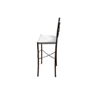
We construct the ShapeNet Holes Test set by selecting models from the ShapeNet test set that have visible holes from any viewpoint. Figure 10 shows several input images for randomly selected models from this subset. This test set is very challenging – many objects have small holes resulting from thin structures; and some objects have holes which are not visible from all viewpoints.

Figure 10: Example input images for randomly selected models from the the Holes Test Set on ShapeNet. For each model we show three different input images showing the model from different viewpoints. This set is extremely challenging – some models may have very small holes (such as the holes in the back of the chair in the left model of the first row, or the holes on the underside of the table on the right model of row 2), and some models may have holes which are not visible in all input images (such as the green chair in the middle of the fourth row, or the gray desk on the right of the ninth row).

References

- [1] Sid Yingze Bao, Manmohan Chandraker, Yuanqing Lin, and Silvio Savarese. Dense object reconstruction with semantic priors. In CVPR, 2013.
- [2] Volker Blanz and Thomas Vetter. A morphable model for the synthesis of 3d faces. In SIGGRAPH, 1999.
- [3] Zhe Cao, Tomas Simon, Shih-En Wei, and Yaser Sheikh. Realtime multi-person 2D pose estimation using part affinity fields. In CVPR, 2017.
- [4] Angel X. Chang, Thomas A. Funkhouser, Leonidas J. Guibas, Pat Hanrahan, Qi-Xing Huang, Zimo Li, Silvio Savarese, Manolis Savva, Shuran Song, Hao Su, Jianxiong Xiao, Li Yi, and Fisher Yu. Shapenet: An information-rich 3d model repository. In CoRR 1512.03012, 2015.
- [5] Christopher B. Choy, Danfei Xu, JunYoung Gwak, Kevin Chen, and Silvio Savarese. 3D-R2N2: A unified approach for single and multi-view 3d object reconstruction. In ECCV, 2016.
- [6] Amaury Dame, Victor A. Prisacariu, Carl Y. Ren, and Ian Reid. Dense reconstruction using 3d object shape priors. In CVPR, 2013.
- [7] Mathieu Desbrun, Mark Meyer, Peter Schröder, and Alan H. Barr. Implicit fairing of irregular meshes using diffusion and curvature flow. In SIGGRAPH, 1999.
- [8] Haoqiang Fan, Hao Su, and Leonidas J. Guibas. A point set generation network for 3d object reconstruction from a single image. In CVPR, 2017.
- [9] Sanja Fidler, Sven Dickinson, and Raquel Urtasun. 3d object detection and viewpoint estimation with a deformable 3d cuboid model. In NeurIPS, 2012.
- [10] David F. Fouhey, Abhinav Gupta, and Martial Hebert. Data-driven 3D primitives for single image understanding. In ICCV, 2013.
- [11] Andreas Geiger, Philip Lenz, Christoph Stiller, and Raquel Urtasun. Vision meets robotics: The kitti dataset. In IJRR, 2013.
- [12] Ross Girshick. Fast R-CNN. In ICCV, 2015.
- [13] Ross Girshick, Jeff Donahue, Trevor Darrell, and Jitendra Malik. Rich feature hierarchies for accurate object detection and semantic segmentation. In CVPR, 2014.
- [14] Benjamin Graham, Martin Engelcke, and Laurens van der Maaten. 3d semantic segmentation with submanifold sparse convolutional networks. In CVPR, 2018.
- [15] Thibault Groueix, Matthew Fisher, Vladimir G Kim, Bryan C Russell, and Mathieu Aubry. A papier-mâché approach to learning 3d surface generation. In CVPR, 2018.
- [16] Saurabh Gupta, Ross Girshick, Pablo Arbeláez, and Jitendra Malik. Learning rich features from rgb-d images for object detection and segmentatio. In ECCV, 2014.
- [17] Richard Hartley and Andrew Zisserman. Multiple view geometry in computer vision. Cambridge university press, 2003.
- [18] Kaiming He, Georgia Gkioxari, Piotr Dollár, and Ross Girshick. Mask R-CNN. In ICCV, 2017.
- [19] Kaiming He, Xiangyu Zhang, Shaoqing Ren, and Jian Sun. Deep residual learning for image recognition. In CVPR, 2016.
- [20] Derek Hoiem, Alexei A. Efros, and Martial Hebert. Geometric context from a single image. In ICCV, 2005.
- [21] Christian Häne, Nikolay Savinov, and Marc Pollefeys. Class specific 3d object shape priors using surface normals. In CVPR, 2014.
- [22] Max Jaderberg, Karen Simonyan, and Andrew Zisserman. Spatial transformer networks. In NeurIPS, 2015.
- [23] Angjoo Kanazawa, Shubham Tulsiani, Alexei A. Efros, and Jitendra Malik. Learning category-specific mesh reconstruction from image collections. In ECCV, 2018.
- [24] Abhishek Kar, Christian Häne, and Jitendra Malik. Learning a multi-view stereo machine. In NeurIPS, 2017.
- [25] Hiroharu Kato, Yoshitaka Ushiku, and Tatsuya Harada. Neural 3D mesh renderer. In CVPR, 2018.
- [26] Alex Kendall, Hayk Martirosyan, Saumitro Dasgupta, Peter Henry, Ryan Kennedy, Abraham Bachrach, and Adam Bry. End-to-end learning of geometry and context for deep stereo regression. In ICCV, 2017.
- [27] Diederik P. Kingma and Jimmy Ba. Adam: A method for stochastic optimization. In ICLR, 2015.
- [28] Diederik P. Kingma and Max Welling. Auto-encoding variational bayes. In ICLR, 2014.
- [29] Thomas N Kipf and Max Welling. Semi-supervised classification with graph convolutional networks. In ICLR, 2017.
- [30] Alex Krizhevsky, Ilya Sutskever, and Geoff Hinton. ImageNet classification with deep convolutional neural networks. In NeurIPS, 2012.
- [31] Abhijit Kundu, Yin Li, and James M. Rehg. 3d-rcnn: Instance-level 3d object reconstruction via render-and-compare. In CVPR, 2018.
- [32] Yangyan Li, Rui Bu, Mingchao Sun, Wei Wu, Xinhan Di, and Baoquan Chen. Pointcnn: Convolution on x-transformed points. In NeurIPS, 2018.
- [33] Joseph J. Lim, Hamed Pirsiavash, and Antonio Torralba. Parsing IKEA Objects: Fine Pose Estimation. In ICCV, 2013.
- [34] Chen-Hsuan Lin, Chen Kong, and Simon Lucey. Learning efficient point cloud generation for dense 3d object reconstruction. In AAAI, 2018.
- [35] Tsung-Yi Lin, Piotr Dollár, Ross Girshick, Kaiming He, Bharath Hariharan, and Serge Belongie. Feature pyramid networks for object detection. In CVPR, 2017.
- [36] Tsung-Yi Lin, Priya Goyal, Ross Girshick, Kaiming He, and Piotr Dollár. Focal loss for dense object detection. In ICCV, 2017.
- [37] Tsung-Yi Lin, Michael Maire, Serge Belongie, James Hays, Pietro Perona, Deva Ramanan, Piotr Dollár, and C. Lawrence Zitnick. Microsoft COCO: Common objects in context. ECCV, 2014.
- [38] Wei Liu, Dragomir Anguelov, Dumitru Erhan, Christian Szegedy, and Scott Reed. SSD: Single shot multibox detector. In ECCV, 2016.
- [39] Jonathan Long, Evan Shelhamer, and Trevor Darrell. Fully convolutional networks for semantic segmentation. In CVPR, 2015.
- [40] William E. Lorensen and Harvey E. Cline. Marching cubes: A high resolution 3d surface construction algorithm. In SIGGRAPH. ACM, 1987.
- [41] Priyanka Mandikal, Navaneet Murthy, Mayank Agarwal, and R. Venkatesh Babu. 3d-lmnet: Latent embedding matching for accurate and diverse 3d point cloud reconstruction from a single image. In BMVC, 2018.
- [42] Lars Mescheder, Michael Oechsle, Michael Niemeyer, Sebastian Nowozin, and Andreas Geiger. Occupancy networks: Learning 3d reconstruction in function space. In CVPR, 2019.
- [43] George A. Miller. Wordnet: A lexical database for english. In Commun. ACM, 1995.
- [44] Georgios Pavlakos, Xiaowei Zhou, Aaron Chan, Konstantinos G. Derpanis, and Kostas Daniilidis. 6-dof object pose from semantic keypoints. In ICRA, 2017.
- [45] Charles R. Qi, Li Yi, Hao Su, and Leonidas J. Guibas. Pointnet++: Deep hierarchical feature learning on point sets in a metric space. In NeurIPS, 2017.
- [46] Joseph Redmon, Santosh Divvala, Ross Girshick, and Ali Farhadi. You only look once: Unified, real-time object detection. In CVPR, 2016.
- [47] Shaoqing Ren, Kaiming He, Ross Girshick, and Jian Sun. Faster R-CNN: Towards real-time object detection with region proposal networks. In NeurIPS, 2015.
- [48] Danilo Jimenez Rezende, S.M. Ali Eslami, Shakir Mohamed, Peter Battaglia, Max Jaderberg, and Nicolas Heess. Unsupervised learning of 3d structure from images. In NeurIPS, 2016.
- [49] Stephan R. Richter and Stefan Roth. Matryoshka networks: Predicting 3d geometry via nested shape layers. In CVPR, 2018.
- [50] Gernot Riegler, Ali Osman Ulusoy, and Andreas Geiger. Octnet: Learning deep 3d representations at high resolutions. In CVPR, 2017.
- [51] Jason Rock, Tanmay Gupta, Justin Thorsen, JunYoung Gwak, Daeyun Shin, and Derek Hoiem. Completing 3d object shape from one depth image. In CVPR, 2015.
- [52] Olga Russakovsky, Jia Deng, Hao Su, Jonathan Krause, Sanjeev Satheesh, Sean Ma, Zhiheng Huang, Andrej Karpathy, Aditya Khosla, Michael Bernstein, Alexander C. Berg, and Li Fei-Fei. ImageNet Large Scale Visual Recognition Challenge. IJCV, 2015.
- [53] Daniel Scharstein and Richard Szeliski. A taxonomy and evaluation of dense two-frame stereo correspondence algorithms. IJCV, 2002.
- [54] Tanner Schmidt, Richard Newcombe, and Dieter Fox. Self-supervised visual descriptor learning for dense correspondence. In IEEE Robotics and Automation Letters, 2017.
- [55] Karen Simonyan and Andrew Zisserman. Very deep convolutional networks for large-scale image recognition. In ICLR, 2015.
- [56] Edward Smith, Scott Fujimoto, and David Meger. Multi-view silhouette and depth decomposition for high resolution 3d object representation. In NeurIPS, 2018.
- [57] Edward J. Smith, Scott Fujimoto, Adriana Romero, and David Meger. GEOMetrics: Exploiting geometric structure for graph-encoded objects. In ICML, 2019.
- [58] Shuran Song and Jianxiong Xiao. Deep Sliding Shapes for amodal 3D object detection in RGB-D images. In CVPR, 2016.
- [59] Hang Su, Varun Jampani, Deqing Sun, Subhransu Maji, Evangelos Kalogerakis, Ming-Hsuan Yang, and Jan Kautz. SPLATNet: Sparse lattice networks for point cloud processing. In CVPR, 2018.
- [60] Xingyuan Sun, Jiajun Wu, Xiuming Zhang, Zhoutong Zhang, Chengkai Zhang, Tianfan Xue, Joshua B. Tenenbaum, and William T. Freeman. Pix3d: Dataset and methods for single-image 3d shape modeling. In CVPR, 2018.
- [61] Christian Szegedy, Wei Liu, Yangqing Jia, Pierre Sermanet, Scott Reed, Dragomir Anguelov, Dumitru Erhan, Vincent Vanhoucke, and Andrew Rabinovich. Going deeper with convolutions. In CVPR, 2015.
- [62] Maxim Tatarchenko, Alexey Dosovitskiy, and Thomas Brox. Octree generating networks: Efficient convolutional architectures for high-resolution 3d outputs. In ICCV, 2017.
- [63] Maxim Tatarchenko, Jaesik Park, Vladlen Koltun, and Qian-Yi Zhou. Tangent convolutions for dense prediction in 3d. In CVPR, 2018.
- [64] Yonglong Tian, Andrew Luo, Xingyuan Sun, Kevin Ellis, William T. Freeman, Joshua B. Tenenbaum, and Jiajun Wu. Learning to infer and execute 3d shape programs. In ICLR, 2019.
- [65] Alexander Toshev and Christian Szegedy. Deeppose: Human pose estimation via deep neural networks. In CVPR, 2014.
- [66] Shubham Tulsiani and Jitendra Malik. Viewpoints and keypoints. In CVPR, 2015.
- [67] Shubham Tulsiani, Hao Su, Leonidas J. Guibas, Alexei A. Efros, and Jitendra Malik. Learning shape abstractions by assembling volumetric primitives. In CVPR, 2017.
- [68] Shubham Tulsiani, Tinghui Zhou, Alexei A. Efros, and Jitendra Malik. Multi-view supervision for single-view reconstruction via differentiable ray consistency. In CVPR, 2017.
- [69] Nanyang Wang, Yinda Zhang, Zhuwen Li, Yanwei Fu, Wei Liu, and Yu-Gang Jiang. Pixel2Mesh: Generating 3D mesh models from single RGB images. In ECCV, 2018.
- [70] Peng-Shuai Wang, Chun-Yu Sun, Yang Liu, and Xin Tong. Adaptive O-CNN: a patch-based deep representation of 3d shapes. In SIGGRAPH Asia, 2018.
- [71] Jiajun Wu, Yifan Wang, Tianfan Xue, Xingyuan Sun, Bill Freeman, and Josh Tenenbaum. Marrnet: 3d shape reconstruction via 2.5 d sketches. In NeurIPS, 2017.
- [72] Jiajun Wu, Chengkai Zhang, Tianfan Xue, Bill Freeman, and Josh Tenenbaum. Learning a probabilistic latent space of object shapes via 3d generative-adversarial modeling. In NeurIPS, 2016.
- [73] Jiajun Wu, Chengkai Zhang, Xiuming Zhang, Zhoutong Zhang, William T. Freeman, and Joshua B. Tenenbaum. Learning 3D Shape Priors for Shape Completion and Reconstruction. In ECCV, 2018.
- [74] Yu Xiang, Roozbeh Mottaghi, and Silvio Savarese. Beyond pascal: A benchmark for 3d object detection in the wild. In WACV, 2014.
- [75] Xinchen Yan, Jimei Yang, Ersin Yumer, Yijie Guo, and Honglak Lee. Perspective transformer nets: Learning single-view 3d object reconstruction without 3d supervision. In NeurIPS, 2016.
- [76] Xiuming Zhang, Zhoutong Zhang, Chengkai Zhang, Joshua B. Tenenbaum, William T. Freeman, and Jiajun Wu. Learning to Reconstruct Shapes from Unseen Classes. In NeurIPS, 2018.