Training large-scale ANNs on simulated resistive crossbar arrays

Abstract

Accelerating training of artificial neural networks (ANN) with analog resistive crossbar arrays is a promising idea. While the concept has been verified on very small ANNs and toy data sets (such as MNIST), more realistically sized ANNs and datasets have not yet been tackled. However, it is to be expected that device materials and hardware design constraints, such as noisy computations, finite number of resistive states of the device materials, saturating weight and activation ranges, and limited precision of analog-to-digital converters, will cause significant challenges to the successful training of state-of-the-art ANNs. By using analog hardware aware ANN training simulations, we here explore a number of simple algorithmic compensatory measures to cope with analog noise and limited weight and output ranges and resolutions, that dramatically improve the simulated training performances on RPU arrays on intermediately to large-scale ANNs.

1 Introduction

The amount of computation needed to train modern deep learning networks is immense. Recently, it has been suggested to use resistive crossbar arrays to accelerate parts of the ANN training in analog space, with a potential dramatic increase in computational performance compared to digital systems [18, 2, 3, 1, 7, 8]. While analog crossbar arrays, also termed resistive processing units (RPU) arrays [7], could speedup inference of DNNs (deep neural networks) and CNNs (convolutional neural networks) [15, 17], the true benefit of an analog deep learning accelerator lies in the acceleration of the training process as well, since training of ANNs is generally orders of magnitude more computationally demanding than inference. However, many significant design, material, and algorithmic challenges still need to be addressed in order to enable training on RPUs with high accuracy.

While forward and backward pass of the stochastic gradient descent (SGD) are relatively straightforward to implement in analog hardware, a truly in-memory weight update that matches the performance of backward and forward passes in computing a pass in constant time, is much more challenging. A fully parallized update is important, however, because if the gradients were instead be computed in the digital part of the system, it would require on the order of $n^{2}$ computations and thus all speed advantages of the analog (i.e. computing the forward and backward in constant time), would be lost.

One promising design is to use stochastic pulse sequences to incrementally update the weight elements in a parallel fashion [7]. This approach was explored for small to moderate DNNs and CNNs[7, 5, 14], as well as LSTMs [6] in simulations. It was shown that moderate amounts of analog noise and physically limited weight update sizes can be tolerated during training, in particular, if one introduces additional noise and bound management techniques, that mitigate the analog noise in the backward pass and can be computed in linear time.

It was also noticed, however, that it is critical for the SGD algorithm to employ device materials that have symmetric switching behavior [7], in other words, a single update pulse in positive or negative direction should effectively change the weight by a similar amount at least on average. To achieve this balanced update behavior requires significant efforts on the material development for RPUs or significant changes in gradient decent algorithms or network architectures.

Another problem is the limited weight ranges and limited number of states supported by the device material, which, in floating point terms, is related to the bit resolution of the weights. Although the resistance of the memristive device can be set to any analog value in principle, materials are inherently subject to noise, and hardware designs require that the weight update is pulsed, where each pulse will increase or decrease the weight value by an finite amount of $dwmin$ on average. Thus, if the weight is bounded in the range $w\in[-w_{b},w_{b}]$, the number of states can be defined as $N_{s}\equiv\frac{2w_{b}}{\Delta w_{\text{min}}}$. Note, however, that cycle-to-cycle variation of the weight update is generally large and the read out process is noisy, too, so that a single read might not be able to discern neighboring states.

In this paper, we focus on the latter issues, that is the limited number of material states, restricted weight ranges, and the noise in the training process. We here ask the following questions: even if we had a device with noisy but (on average) ideally symmetric switching behavior, how many states are necessary to successfully train larger scale models on more challenging image data sets (than MNIST)? Are there simple ways to improve performance on RPU arrays with their limited weight resources?

Our contribution are: (1) Scaling up the hardware realistic pulsed-update training on simulated RPUs to larger networks with $>60$ million weights and $>1.2$ million images, such as AlexNet on the ImageNet data set [13], (2) showing the importance of normalization to overcome analog noise, (3) devising a new scheme for virtually remapping the weight ranges to maximize usable resistive states and achieving proper regularization on RPUs arrays.

Figure 1: Backward pass and pulsed update for RPU arrays hardware implementation, adopted from [7]. Forward pass is analogous to the backward pass (with input and output reversed). (Left) Matrix-vector operation are performed in analog space, where memristors encode the weights of the matrix and inputs are encoded temporally with voltage pulses of variable length. (Right) During update cycle, stochastic pulse trains are generated, where the probability of pulse occurrence encodes the input values. If pulses from both input sides coincide at a RPU device, its resistive value is updated corresponding to (on average) $\Delta w_{\text{min}}$ in weight units.

2 RPU model and simulations

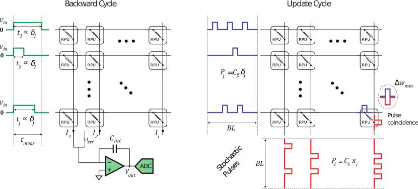
Our simulation is based on the RPU model proposed by [7] (see Fig. 1 for an illustration). We, however, adapted the previous C++-simulator of [7] to integrate with the Caffe2 machine learning framework [12], to be able to flexible handle different network architectures and datasets. We also re-implemented the RPU simulation code to fully support GPUs acceleration to improve the runtime for larger models and convolutions for inference and training. For the ConvNets investigated below, a training simulation with fully pulsed update typically only runs 2-3 times slower than a native floating point training in Caffe2.

We adopt the scheme of [5] and use stochastic pulse trains of maximal length 31. We ensured in our simulation that pulsed weight update is done (1) by drawing actual stochastic pulse trains for each update and calculating the coincidence of pulses per weight, (2) for every coincident pulse occurrence the corresponding device weight (conductance) is updated by a single step drawn from a Gaussian distribution (with standard deviation 30% of the mean $\Delta w_{\text{min}}$) and saturating the hard bounds if necessary, (3) the sequence order of updates (in case of a batch learning or convolutions) is preserved as if would be done in hardware.

In our simulations, all analog noise, such as circuit components and peripheral noise, is referred to the output of the analog computation and modeled as Gaussian noise processes added to each analog output line. The noise values are re-drawn for each analog computing step, i.e. each computed vector-matrix product. The device specification in [7] gives reasons to set the standard deviation of these cumulative noise terms to $0.06$.

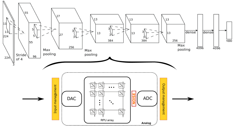
Additionally, we assume that each analog RPU array stores the weights of a layer (the kernel matrix) and performs matrix vector products in a way described in [7, 5]. The RPU array is communicating with the next layer in digital space, thus we assume analog-to-digital (ADC) and digital-to-analog (DAC) converters per RPU array (see Fig. 2). The DAC/ADC discretizes the input values into $m$ bins in the range of its bounds (which are fixed by hardware design to $\pm 1$ for DAC, and $\pm 12$ for the ADC, see our definition of the baseline RPU model [5]). The bit resolution of the converters are then $\log_{2}m$. We here assume 7 bit for DAC and 9 bit for ADC if not stated otherwise (see also [6] for a discussion).

For the SGD training, we just use plain batch-wise SGD without any additional momentum or weight decay, which would be difficult to efficiently implement on analog hardware architectures.

Figure 2: In the RPU simulations Caffe2 fully-connected and convolution layers are replaced by operators that contain the analog hardware simulation. Given a network architecture, e.g. AlexNet [13] in this illustration, each layer will be translated to a separate RPU operator (of matching sizes of the weight matrices). The RPU operator contains input and output management in the digital part, where inputs are normalized or scaled by the maximal input value in floating point precision, as described in the text. DAC and ADC have limited ranges and precision and the analog noise is drawn each operation cycle from a Gaussian distribution and added to each analog output line (see [7] for details of our RPU model).

2.1 Noise, bound, and update management techniques

It has been shown previously [5] that it is essential to introduce noise management techniques on the digital side, to cope with the noisy analog computations as well as the bounded ranges of the inputs and outputs of the analog RPU.

Noise management becomes vitally important during backward pass, since the backward propagated errors are usually orders of magnitude smaller than the forward pass values and would be buried in the analog noise floor if not properly re-scaled. In particular, we use the noise management introduced by [5], where the digital input vector $\mathbf{x}$ is divided by $\alpha=\max|x_{i}|$ before the DAC and re-scaled again by $\alpha$ after the ADC in digital. Additionally, we use a bound management (only in the forward pass), that iteratively multiplies $\alpha$ by factors of 2 until the ADC bound does not saturate any of the outputs anymore. In this way, larger output values can be accommodated, with the cost of ADC resolution (which is effectively reduced by a factor of 2 for each iteration) and cost of runtime since the computation of the forward pass is essentially repeated multiple times. However, since one cycle is very fast (order of 100ns) and the geometric reduction of $\alpha$ does not need many iterations (at the very most the number of bits of the ADC), the additional runtime cost seems tolerable if necessary for high accuracy, which is in particular important before the softmax layer. Also, hardware solutions could cut short the integration time further, by triggering an abort when one output saturates early.

In addition, we use an update management introduced in [5], that rescales the pulse generation probabilities based on the $\max|x_{i}|$ and $\max|d_{j}|$ and the expected pulse width $\Delta w_{\text{min}}$, where $\mathbf{d}$ denotes the error vector during update. We refer to [5] for the details.

3 Results

We first investigated a small 3-layer convolutional network plus one fully-connected layer and ReLu activation on the CIFAR10 data set (with weak data augmentation, e.g. mirroring and color jittering). The network has 79328 weights and uses lateral response normalization (LRN) between convolution layers. The image size is $32\times 32$ pixels. While of similar model and data size as the CNN previously investigated on the MNIST data set [5], the CIFAR-10 dataset contains rescaled color images, whose classification is much more challenging than classifying the cleanly handwritten binary digits of MNIST: Using floating point (FP) and no input data augmentation, the above CNN achieves about 0.8% test error on MNIST, while only 25% test error on CIFAR-10.

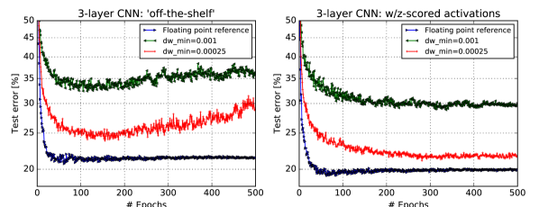
We first trained the network with our baseline RPU model (see [5] for definition), except with balanced weight update and 7 bit DAC and 9 bit DAC resolutions. This RPU model has 1200 weight states on average per device ($\Delta w_{\text{min}}=0.001$ and $w_{b}=0.6$) and gave very acceptable performance for a smaller CNN on MNIST (compare to [5] Figure 4, “All no imbalance”). Nevertheless, here we found that performance is dramatically impaired, see Fig. 3 (left, green curve), albeit using the same bound and noise management techniques described in [5]. Even increasing the number of available states by $4\times$ does not reach FP performance (Fig. 3, left, red curve).

Thus, more challenging data sets and larger networks seem to again require additional algorithmic improvements for training RPUs. In the following, we introduce two simple remedies.

Figure 3: 3-layer CNN network on CIFAR10 trained with the baseline RPU model [5], except using balanced switching behavior. (Left) Using the ’off-the-shelf’ model with the RPU simulation for each layer, performance is severely impaired compared to the floating point reference, even if the number of states is increased $4\times$ (red line). (Right) Normalization of the (digital) activations between layers improves RPU performance and eliminates overfitting (ie. late rise in test error, see left). Parameters: $\lambda=0.1$, multiplied by 0.8 every 20 epochs; no weight decay; batch size 100.

3.1 Normalization balances activations in the presence of noise

The reason for the poor learning ability becomes clear when estimating the signal-to-noise ratio of the analog matrix product. For each analog output, we have $y_{i}=\mathbf{w}_{i}\mathbf{x}+\xi$, where $\mathbf{w}_{i}$ is the $i$th row of the analog weight matrix and $\xi$ the analog noise term, i.e. a Gaussian process with zero mean and standard deviation $\sigma$. If we assume that $\mathbf{w}_{i}$ is a “good” feature vector for input $\mathbf{x}$, the direction of $\mathbf{x}$ and $\mathbf{w}_{i}$ should approximately match, thus $\mathbf{w}_{i}\approx\frac{\left\lVert\mathbf{w}_{i}\right\rVert}{\left\lVert\mathbf{x}\right\rVert}\mathbf{x}$. Thus for a number of similarly well matching inputs, the signal-to-noise ratio $\frac{\langle y_{i}^{2}\rangle}{\sigma^{2}}$ is roughly

$$\text{SNR}\propto\frac{\left\lVert\mathbf{w}_{i}\right\rVert^{2}\langle\left\lVert\mathbf{x}\right\rVert^{2}\rangle}{\sigma^{2}}.$$ (1)

Although this is only an approximate calculation, it shows that weight vectors, that are well matched with the inputs, will quickly grow in norm to improve the signal-to-noise ratio during initial SGD training.

Moreover, since only few rows of $W$ matches the input initially well, they will outgrow others quickly, leaving the norms of the rows of $W$ very unbalanced. Note that this is in particular problematic with the RPU noise management, since the inputs are divided by $\max|x_{i}|$ so that weakly activated inputs get buried in the output noise. If they are suppressed to such a degree that the output becomes smaller than the smallest ADC resolution, they may become essentially zero in the output.

Thus we propose here to counter-act this drive to unbalance rows of $W$ by using (channel-wise) normalization of the input (z-scoring). Note that this is very similar to spatial batch normalization (BN) used by default (for other reasons) in modern deep learning architectures, such as ResNet [10]. However, since we here simply want to maintain the variance across the inputs, we do not train an additional scale or bias per channel, like typically done in BN [11], and we place the normalization before each layer. Additionally, we z-score the inputs across the batch before a fully-connected layer, not only convolutions. As in BN, during testing we use running mean and variances from the train runs and are fixed during testing.

With this modification of the network structure, where we replace the LRN with activation z-scoring, we find that the 3-layer CNN even beats the original model (using LRN) considerably, when trained in software with floating point accuracy without any RPU hardware simulations or noise (with identical learning rate and without weight decay), see Fig. 3 (right, blue curve).

More importantly, the baseline RPU model now performs much more stable, and at least the model with $4\times$ more states almost reaches FP performance Fig. 3 (right, red curve). However, the baseline RPU model with more limiting number of weight states is still 10% off the FP reference (green curve).

3.2 “Virtually” remap weight ranges to maximize usable states

Our second suggestion is to “virtually” remap the weight bounds to an usable weight range per layer, which not only maximizes the available physical states, but also has the additional benefit that saturation at the weight bounds acts as n adequate weight regularization. The motivation comes from the following observation.

Between layers of a deep network, it is important to approximately maintain a 1:1 ratio of the standard deviation of the input and outputs of a layer. In particular, assume that $y_{j}=\sum_{i=1}^{n}w_{ji}x_{i}$ and $x_{i}\sim{\cal N}(0,1)$ behaves like a standard normal random variable. Let’s for simplicity assume that the matrix $W$ has all identical entries $w$. Then, it is easy to see that the output standard deviation is of the order of $\sqrt{n}$, i.e. $y_{j}\sim{\cal N}(0,w\sqrt{n})$. Thus, the standard deviation of the output is proportional to the square root of number of dimensions of the input. This idea, which also holds for more general $W$, is the basis for all weight initialization techniques, such as Xavier or He initialization [4, 9]. In Caffe2’s Xavier implementation, the weight is initialized uniformly in the range $w\in\left(-\frac{\sqrt{3}}{\sqrt{n}},+\frac{\sqrt{3}}{\sqrt{n}}\right)$. Note that the division by $\sqrt{n}$ achieves that the output standard deviation is roughly of the order of the input standard deviation, independent of the number of column of the weight matrix.

Such weight initializations were shown to be very essential in successful training of deep ANNs, as it prevents an explosion of the activations through the layers and normalizes for different weight matrix sizes [4, 9].

Figure 4: Same network and settings as in Fig. 3 but now additionally applying the described weight scaling. (Left) Using the original 3-layer CNN with RPU simulation. Note that proper weight scaling makes the RPU network actually beat the performance of the FP performance, when using $4\times$ more states (red), and dramatically improve the baseline RPU model with more limited number of states. (Right) Using the z-scored network in combination with the weight scaling does not further improve the RPU simulations for this network. Parameters: as in Fig. 3, $\gamma=0.4$

3.2.1 Proper weight scaling for RPUs

We propose to take advantage of the requirement of scaling the weight into a smaller range for larger weight matrices. The insight is that, even for a trained model the requirement of having the similar input and output standard deviation should still hold. Thus individual weights should not deviate “too much” from their initialization bounds. That means after training it is still $\max|w_{ij}|=\frac{\beta}{\sqrt{n}}$ with $\beta\approx 1$ or at most a few times larger than that. Given the limited weight resources in analog space, we thus do not need to waste weight states to code for weight values $\gg\frac{1}{\sqrt{n}}$. Our approach is thus to virtual map the weight range $(-\frac{\beta}{\sqrt{n}},\frac{\beta}{\sqrt{n}})$ into the original weight range $(-w_{b},w_{b})$. This can be achieved in the RPU array by adjusting the mapping of weight values to resistive values accordingly without changing the hardware specifications. Or it could be done in digital, by additional scaling the digital output of the RPU calculation (of forward and backward passes) by a factor of $\frac{\beta}{\sqrt{n}w_{b}}$, to virtually re-scale the weight range. Note that in this case the learning rate $\lambda$ has to be divided by the same factor for that particular layer, to re-scale it properly to the re-mapped weight range.

We use $\beta\equiv\frac{\sqrt{3}}{\gamma}$ (with $\gamma\leq 1$) for all layers if not otherwise stated, and initialize the weights uniformly in the range $(-\gamma w_{b},\gamma w_{b})$. Thus we allow the weights to grow $\frac{1}{\gamma}$ times beyond the maximal initialization value and therefore maximize the number of available states in this range. Note that we use the bound management to ensure that signals are not saturated because of the limited output range (see above).

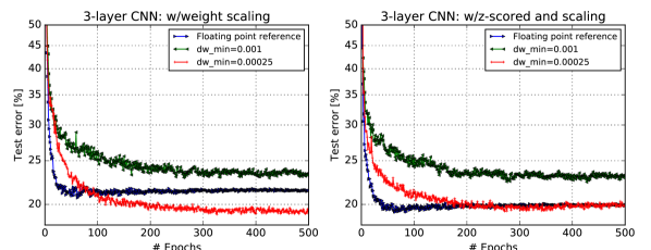
We trained the 3-layer CNN again using the above scaling and normalization approaches. We find that, in particular when the number of states is more limited (e.g. 1200 for the baseline RPU model), scaling the weight bounds properly is the most effective to increase performance (see Fig. 4, left). In this network architecture, the performance increased by least 10 %-points. Moreover, the RPU now is much better regularized (no late increase in test error as in Fig. 3 left), as the saturation at the limited weight range prevents individual weights to become dominating.

The weight scaling approach seems to also normalize the activation correctly, so that z-scoring does not gain on top of using the weight scaling (compare Fig. 4 right).

Note that when the number of states is increased 4-fold, the RPU model in fact now beats the floating point reference, despite the noise and pulsed weight update, because of better regularization properties. In conclusion, the weight scaling forces the RPU to operate on the correct weight range and maximizes the available states in this range. Thus, the requirement for the amount of states is lessened.

3.3 Larger networks and data sets

3.3.1 ResNet on CIFAR

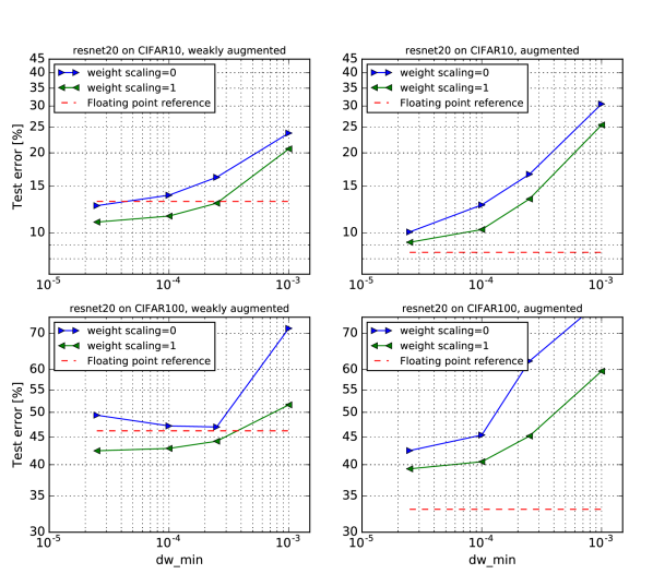
We further investigated the number of states needed for training ResNet20 (i.e. $n=3$ in [10] 4.2) on CIFAR10 and CIFAR100 data sets. We use the above weight scaling technique. Note that ResNet has batch normalization per default which we use here instead of the z-scoring (results are slightly better for BN in case of ResNet). We applied weight scaling and varied the number of states of our baseline RPU model (by changing $\Delta w_{\text{min}}$) and found that (see Fig. 5) (1) weight scaling improves the performance considerably, in particular, when the number of states is smaller, (2) with weak data augmentation, pulsed update RPU generalizes better than the FP reference, (3) with strong data augmentation (30% scale jitter with random cropping, and random image shuffling per epoch) the RPU model needs at least $48$K states to be able to come close to the FP reference, which improves dramatically with stronger data augmentation.

Our results indicates that larger networks and more challenging tasks (such as CIFAR100) demand more resources in terms of number of states. In particular, analog noise and finite number of states seem to limit the performance gain achieved by strong data augmentation, which is very effective method for improving generalizability for ANNs trained with floating point accuracy and limited dataset sizes.

Figure 5: Training on Resnet20 (18 conv layers) on CIFAR10 (upper plots) and CIFAR100 (lower plots). Left plots uses weak augmentation as before (color jitter and random mirroring), where as use stronger input augmentation (scale jitter 1.3 times and random order shuffeling). Note that 4x times more states than the baseline RPU model is enough to beat the floating point reference, when using weight scaling. However, while input augmentation strongly improves the floating point accuracy, it improves the RPU network less well (and actually significantly reduces the performance in case of $\Delta w_{\text{min}}=0.001$), potentially because the input becomes too erratic for the noisy pulsed update process. Higher number of states, recover the lost performance to some degree. Parameters: best of $\lambda=0.2$ or $\lambda=0.4$, multiplied by a factor each 150 epochs so that 1% of $\lambda$ is reached after the 500 epochs training; batch size 100; $\gamma=1$.

3.3.2 AlexNet on Imagenet

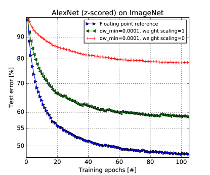
For the first time, we simulate analog network training on close to state-of-the-art scale using pulsed weight update and noisy backward pass within the specification of analog RPUs. We train AlexNet [13] from scratch on the Imagenet database, a problem, that is more than 40000 times more challenging than training LeNet on MNIST (in terms of MACs per epoch), which nevertheless is still used as a typical benchmark for analog hardware evaluation [16].

We find that using AlexNet off-the-shelf is not trainable with our baseline RPU model (even with floating point update but limited ADC/DAC resolution, not shown). We thus applied the above z-scoring techniques between each layer and tested the effect of additionally using weight scaling on the number of device states necessary. In Fig. 6 we show that, using 12K states during pulsed update ($\Delta w_{\text{min}}=0.0001$, 10x more states than our baseline RPU model), reaches top-1 test error of only slightly below 80%. On the other hand, enabling weight scaling, we find that the test error is dramatically improved, by about 20 %-points, reaching test errors of slightly below 60%. That this positive effect of weight remapping is larger for AlexNet than for ResNet is understandable since the dimensions of the weight matrices (and therefore the scale term proportional to $\sqrt{n}$) is much larger (up to 9216) than for ResNet on CIFAR (up to 577).

However, our results also indicate that for reaching the floating point accuracy of below 50%, 12K states are not enough. Thus, although our approach dramatically improves accuracy of analog approaches, even with symmetric updates, reaching floating point accuracy with analog hardware on larger scale networks remains a challenge and probably requires additional algorithmic improvements similar to those presented here.

Figure 6: Training on AlexNet on ImageNet with (symmetric) pulsed update and z-scored activations. Effective number of states is 12K, otherwise the baseline RPU model is used as above. Note that enabling the weight scaling dramatically improves training performance. However, even with weight scaling, 12K states are not enough to reach FP performance. Parameters: $\lambda=0.00125$, multiplied by 0.8 every 15 epochs; only weak augmentation; batch size 25.

4 Conclusion

Scaling up simulations of analog crossbar approaches for acceleration of ANN training is a necessary and essential prerequisite for evaluating and finding new algorithmic or hardware design solutions that minimize the accuracy gap in respect to the floating point reference. We show that simple algorithmic modifications, such as proper normalization and weight range remapping, can dramatically improve training performance on large-scale ANNs with constraint weight resources (range and precision).

Our results also highlight the importance of having a digital part between layers that could accommodate not only the activation functions and pooling, but also the essential bound and noise managing techniques, and other algorithmic compensatory measures such as normalization and weight remapping as suggested here. To maintain the advantages of the crossbar architecture, these digital operations need to be computed locally close to the array’s peripheral edges.

While our algorithmic improvements yield a considerable improvement in performance of training in-memory on analog RPU arrays, the number of required states to match the FP reference for large scale networks is still beyond current materials [8]. However, possible solution pathways exist, e.g. one RPU device might be a combination of multiple physical devices (of possibly different significance), which could dramatically enlarge the number of attainable states (e.g. as in [15, 1]).

Note that the ConvNets evaluated here are generally not well suited for analog architectures because of the re-use of the kernel matrix, which slows down computation in analog systems (see [14] for a discussion). However, [14] also suggested an algorithmic modification of ConvNets to overcome this problem and better map the ConvNet architecture to analog RPU systems by replicating kernel matrices and train them in parallel. How noise and limited number of states are effected in these so-called RAPA-ConvNets remains to be investigated.

While we here have simulated the training process on RPU arrays, a related problem is training ANNs in a RPU hardware-aware manner, to optimize the inference performance on RPU devices. These simulation would include all components used in our simulations, except that the weight update and backward pass would be considered perfect and noise-free, which would dramatically improve the attainable accuracy, even with much less available states or more noise in the forward pass. Thus, training in analog space is a much more challenging problem than training to optimize inference on analog RPUs.

In summary, we here explored the challenges of analog hardware design constraints for training large-scale networks and suggested a number of algorithmic compensatory measures to lessen the performance impacts of noise, limited number of states and limited weight ranges, even if the device switching behavior would be ideal, as assumed here. While we show a dramatic improvement, our results also suggest that more concentrated research efforts on algorithmic, material, and system-level are needed to be able reach state-of-the-art training performance of analog ANN accelerators.

References

- [1] S. Ambrogio, P. Narayanan, H. Tsai, R. M. Shelby, I. Boybat, C. Nolfo, S. Sidler, M. Giordano, M. Bodini, N. C. Farinha, et al. Equivalent-accuracy accelerated neural-network training using analogue memory. Nature, 558(7708):60, 2018.
- [2] G. W. Burr, R. M. Shelby, A. Sebastian, S. Kim, S. Kim, S. Sidler, K. Virwani, M. Ishii, P. Narayanan, A. Fumarola, et al. Neuromorphic computing using non-volatile memory. Advances in Physics: X, 2(1):89–124, 2017.
- [3] A. Fumarola, P. Narayanan, L. L. Sanches, S. Sidler, J. Jang, K. Moon, R. M. Shelby, H. Hwang, and G. W. Burr. Accelerating machine learning with non-volatile memory: Exploring device and circuit tradeoffs. In Rebooting Computing (ICRC), IEEE International Conference on, pages 1–8. Ieee, 2016.
- [4] X. Glorot and Y. Bengio. Understanding the difficulty of training deep feedforward neural networks. In Proceedings of the thirteenth international conference on artificial intelligence and statistics, pages 249–256, 2010.
- [5] T. Gokmen, M. Onen, and W. Haensch. Training deep convolutional neural networks with resistive cross-point devices. Frontiers in neuroscience, 11:538, 2017.
- [6] T. Gokmen, M. Rasch, and W. Haensch. Training lstm networks with resistive cross-point devices. Frontiers in neuroscience, 12:745, 2018.
- [7] T. Gokmen and Y. Vlasov. Acceleration of deep neural network training with resistive cross-point devices: design considerations. Frontiers in neuroscience, 10:333, 2016.
- [8] W. Haensch, T. Gokmen, and R. Puri. The next generation of deep learning hardware: Analog computing. Proceedings of the IEEE, 107(1):108–122, 2019.
- [9] K. He, X. Zhang, S. Ren, and J. Sun. Delving deep into rectifiers: Surpassing human-level performance on imagenet classification. In Proceedings of the IEEE international conference on computer vision, pages 1026–1034, 2015.
- [10] K. He, X. Zhang, S. Ren, and J. Sun. Deep residual learning for image recognition. In Proceedings of the IEEE conference on computer vision and pattern recognition, pages 770–778, 2016.
- [11] S. Ioffe and C. Szegedy. Batch normalization: Accelerating deep network training by reducing internal covariate shift. arXiv preprint arXiv:1502.03167, 2015.
- [12] Y. Jia, E. Shelhamer, J. Donahue, S. Karayev, J. Long, R. Girshick, S. Guadarrama, and T. Darrell. Caffe: Convolutional architecture for fast feature embedding. In Proceedings of the 22nd ACM international conference on Multimedia, pages 675–678. ACM, 2014.
- [13] A. Krizhevsky, I. Sutskever, and G. E. Hinton. Imagenet classification with deep convolutional neural networks. In Advances in neural information processing systems, pages 1097–1105, 2012.
- [14] M. J. Rasch, T. Gokmen, M. Rigotti, and W. Haensch. Efficient convnets for analog arrays. arXiv preprint arXiv:1807.01356, 2018.
- [15] A. Shafiee, A. Nag, N. Muralimanohar, R. Balasubramonian, J. P. Strachan, M. Hu, R. S. Williams, and V. Srikumar. Isaac: A convolutional neural network accelerator with in-situ analog arithmetic in crossbars. ACM SIGARCH Computer Architecture News, 44(3):14–26, 2016.
- [16] V. Sze, Y.-H. Chen, T.-J. Yang, and J. S. Emer. Efficient processing of deep neural networks: A tutorial and survey. Proceedings of the IEEE, 105(12):2295–2329, 2017.
- [17] C. Yakopcic, M. Z. Alom, and T. M. Taha. Extremely parallel memristor crossbar architecture for convolutional neural network implementation. In 2017 International Joint Conference on Neural Networks (IJCNN), pages 1696–1703. IEEE, 2017.
- [18] J. J. Yang, D. B. Strukov, and D. R. Stewart. Memristive devices for computing. Nature nanotechnology, 8(1):13, 2013.